A Self-Test, Self-Calibration and Self-Repair Methodology of Thermopile Infrared Detector

Abstract

To improve the reliability and yield of thermopile infrared detectors, a self-test, self-calibration and self-repair methodology is proposed in this paper. A novel micro-electro-mechanical system (MEMS) infrared thermopile detector structure is designed in this method with a heating resistor building on the center of the membrane. The heating resistor is used as the stimuli of the sensing element on chip to achieve a self-test, and the responsivity related with ambient temperature can be calibrated by the equivalent model between electrical stimuli and physical stimuli. Furthermore, a fault tolerance mechanism is also proposed to localize the fault and repair the detector if the detector fails the test. The simulation results with faults simulated by the Monte Carlo stochastic model show that the proposed scheme is an effective solution to improve the yield of the MEMS thermopile infrared detector.

1. Introduction

MEMS non-contact infrared radiation (IR) temperature detectors have been an effective means on monitoring and detecting body temperature during the COVID-19 pandemic [1,2,3,4,5], which increased the demand of MEMS IR sensors rapidly. High demand and high output mean that there is a greater requirement for product reliability than before [6], including a fast and low-cost test method, mature calibration strategy and related fault analysis and fault repair mechanisms that need to be further explored.

For the testing of MEMS, the most common tool is automatic test equipment (ATE), which is designed for MEMS 3D micromechanical structure devices and provides a peculiar test stimulus such as the shock stimulus, the pressure stimulus, the vibration stimulus [7,8,9,10,11], etc. For the high-precision MEMS infrared thermopile detector, a black body radiation is needed as the stimuli, and a readout circuit is used to obtain signals and evaluate the performance of the device [12,13]. The above test methods are too complicated and costly since each kind of detector needs a specific test stimulus, though those methods can obtain comprehensive performance parameters of devices.

In recent years, built-in self-test (BIST) and built-in self-calibration (BISR) mechanisms of MEMS have been proposed to improve the test efficiency and sensor accuracy and lower test cost [14]. Researchers have investigated a variety of approaches to realize testing and calibration on chips. In 2001, Benoit Charlot summarized how to test sensors with electronical stimuli instead of physical stimuli in a parallel plate capacitance structure, a micro-beam piezoresistive structure and a cantilever beam thermocouple structure, respectively [15]. An interesting structure was designed for a convective accelerometer with a heater built in the middle of two sensing beams, providing the symmetrical temperature gradient, which can detect the bias when there is lack of acceleration [16]. Generally, the MEMS BIST can be summarized into four classes based on different MEMS sensors principles: the test of symmetry, the test of sensitivity, parameter extraction and direct test [17]. Besides, several researchers have attempted to realize calibration on chip. In 2014, Jia et al. proposed an on-chip scheme to calibrate the responsivity of infrared thermopile temperature sensor with digital control signals [18]. Based on this scheme, a machine learning algorithm robust heteroscedastic probabilistic neural network (RHPNN) was also proposed to calibrate the responsivity with the parameters of a read circuit by Kuan et al. [19].

Though the above BIST or BISR methods can achieve testing and calibration of a MEMS detector on-chip, the response of the closed-loop test achieved by electric stimulus can also be further used for the fault analysis and defects repair which has not been addressed well in previous works.

In this paper, a self-test, self-calibration and self-repair scheme for infrared thermopile detectors is established, and the device reliability testing, failure analysis and fault repair are closed-loop processes from a broader perspective. First, the built-in heating resistor is used to generate internal quantitative stimulus, the response signal is analyzed, and the threshold method is used to determine whether the device is faulty. Second, the equivalent relationship between physical stimulus and electrical stimulus can be fitted by the simulation data, so that the thermopile responsivity at different ambient temperatures is corrected by it. Last, the self-repair of thermopile detector can be fault tolerant through the redundancy method, which partitions the thermopile into M identical modules, the fault type and location can be predicted by BP neural network, and the fault module is isolated to keep the detector work normal. The response of electrical stimulus can not only be used to implement testing on-chip, but also to realize the fault tolerance of some fault types to repair detectors. Simultaneously, the responsivity related with ambient temperature can be calibrated by the equivalent model between electrical stimuli and physical stimuli. This ultimately improves the reliability of the device.

This paper is organized as follows: Section 1 is an introduction to the test and calibration of infrared thermopile detectors, and there will present some past solutions for this question. Section 2 introduces the basic principle of MEMS infrared thermopile, and the derivation process of one-dimensional thermal steady-state model for built-in thermal resistor. In Section 3, the design and theoretical basis of self-testing, self-calibration and fault repair are introduced in detail. Section 4 introduces the verification simulation design for the scheme proposed in this article. The simulation results are described in Section 5 and summarized in Section 6.

2. Basic Principles and Analysis

2.1. The Principle of Infrared Thermopile Detector

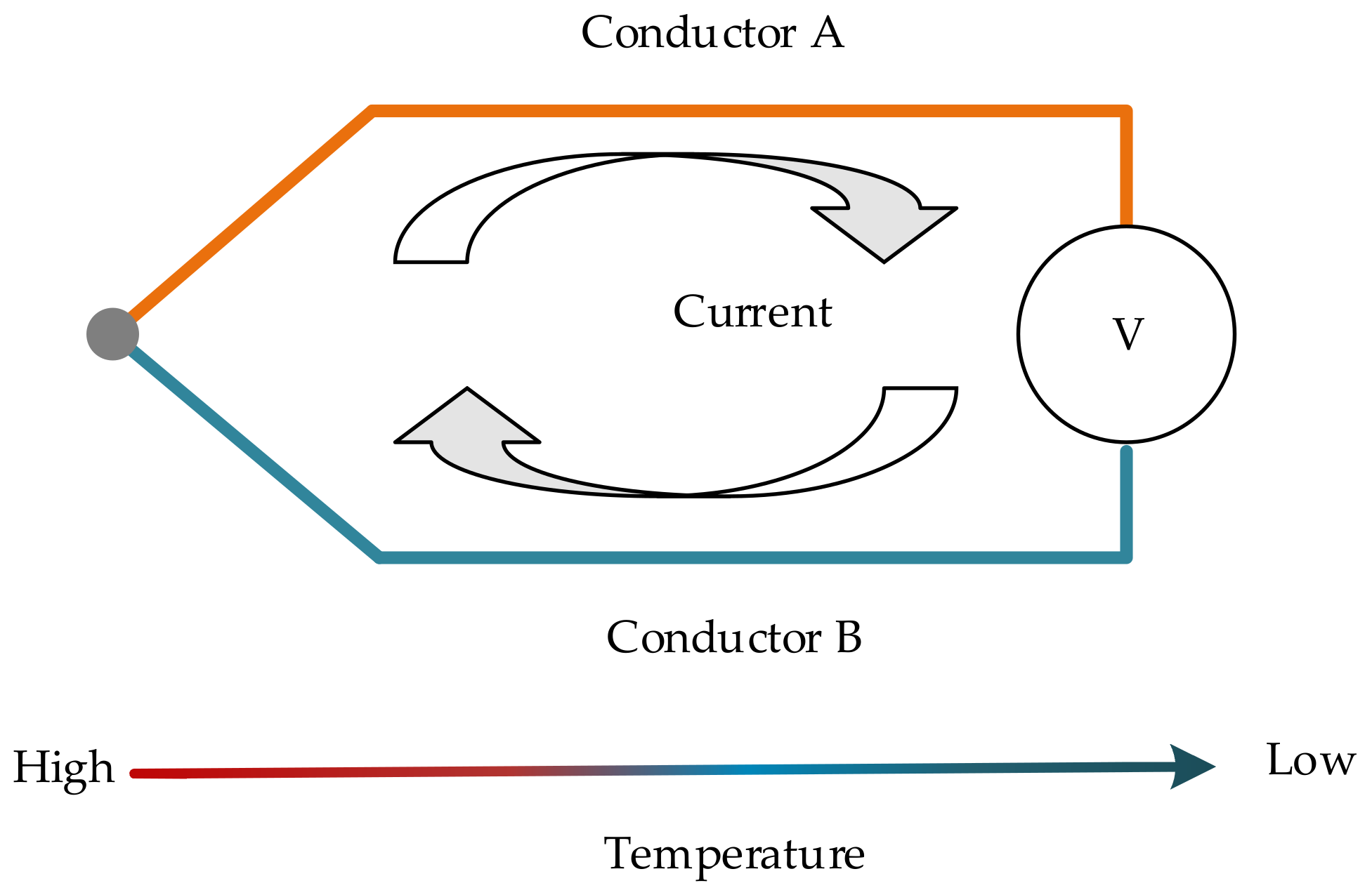
Based on Kirchhoff’s radiation law, energy can transmit by absorbing and emitting the spectrum. In this course, the transmission efficiency relies on the wavelength of the spectrum and the temperature of objects. The thermopile temperature detector is designed based on the Seebeck effect. This effect describes the generation of voltage between the ends of two joint materials (thermocouple) placed on a temperature gradient which has different Seebeck coefficients, as shown in Figure 1.

$$V_{out}=\left({\alpha }_A-{\alpha }_B\right)∆T=\left({\alpha }_A-{\alpha }_B\right)\left(T_{obj}-T_a\right)$$

(1)

where, ${\alpha }_A$, ${\alpha }_B$are the Seebeck coefficients of two different materials respectively, $T_{obj}$ is the temperature of the object and $T_a$ is the ambient temperature.

According to the Seebeck effect, the temperature change of the thermocouple junction end can lead to the change of voltage at the output end, so an infrared thermopile detector can be designed to obtain the temperature of object whose energy can transfer through infrared radiation and increase the temperature of the absorption zone on which the hot end of the thermopile is placed.

According to the Stefan–Boltzmann law, the relationship between blackbody radiation power and its temperature is described, as shown in Equation (2):

$$\mathrm{P}=\mathrm{A}{j}^{*}=A\epsilon \sigma \left(T_1^4-T_2^4\right)$$

(2)

where A is the area of the absorption region, ε is the emissivity of the grey body and σ is the Stefan–Boltzmann constant, the value of the constant is:

$$\mathsf{\sigma }=\frac{2{\pi }^5{k}^4}{15c^2{h}^3}$$

(3)

where k is the Boltzmann constant, h is Planck’s constant, and c is the speed of light in a vacuum.

Defined the responsivity of thermopile R:

$$\mathrm{R}=\frac{∆V}{P}$$

(4)

where P is the power of absorbed radiation.

The temperature of object can be calculated by the following formula:

$$T_{obj}=\sqrt[4]{\frac{∆V}{ARk}+T_a^4}$$

(5)

where $∆V$ is obtained from readout circuit, $T_a$ is the ambient temperature calculated by the value of the thermistor isolating from the thermopile and R changes with $T_a$.

2.2. Physical Stimulus and Electrical Stimulus Mechanism

It can be seen from Equation (1) that the principle of the infrared thermopile detector is to convert infrared radiation energy into electrical energy through the Seebeck effect, so the temperature can be characterized by output electrical signals. Therefore, the infrared thermopile detector is designed based on this theory.

Thermopile infrared detectors usually consist of three parts: thermocouple, dielectric support layer and heat dissipation substrate. Usually the thermopile infrared detectors have three structures: 1. Closed membrane structure; 2. Cantilever beam structure; 3. Suspended structure. From the performance comparison of the three structures, the thermopile infrared detector with the closed membrane structure has the smallest thermal resistance, and its response time is the shortest compared with the other two structures; the thermopile infrared detector with the suspended structure has the highest thermal resistance and the longest response time; the performance of the cantilever structure is between these two structures. From a process point of view, the preparation of the closed membrane structure detector is the easiest, and the preparation process of the cantilever-beam structure detector is the most complicated. The thermopile infrared detectors with closed membrane structure currently on the market have a simple structure, but the yield rate is low. In summary, the closed membrane structure of the thermopile detector is used as the research object of this article.

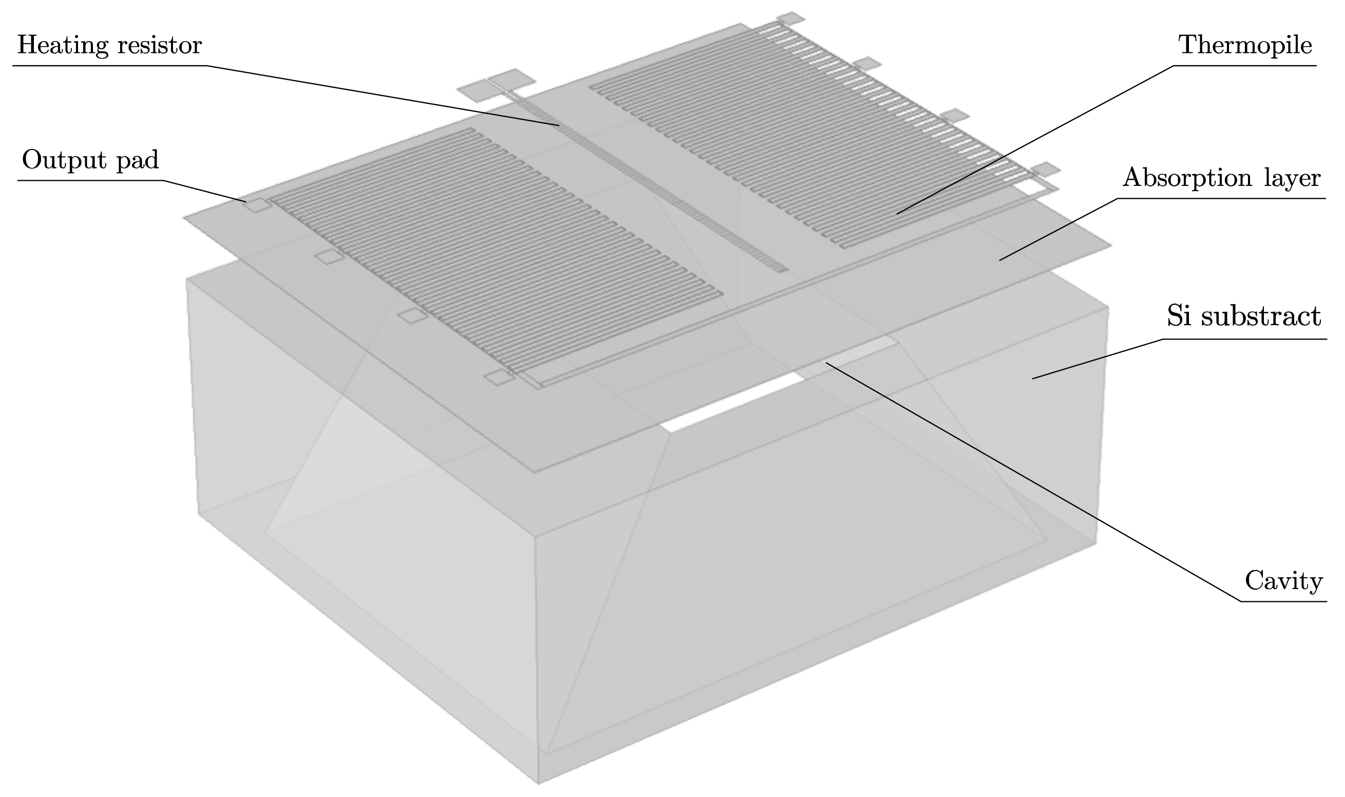
In the closed membrane thermopile structure, as shown in Figure 2, the infrared radiation of the object produces a temperature distribution in the absorption layer, and the temperature gradient can be detected by the thermopile to calculate the object temperature by Equation (4).

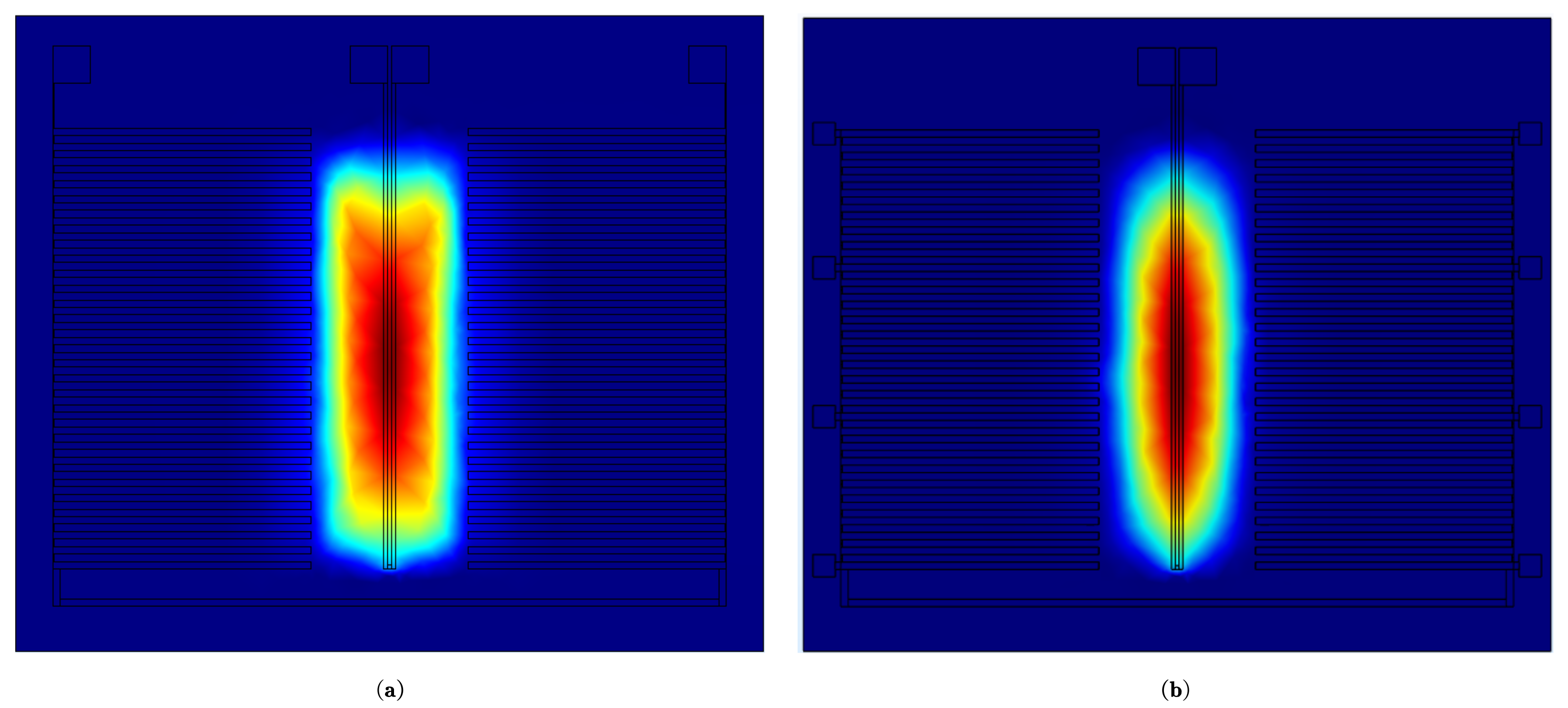
For infrared thermopile detectors, the process of the temperature gradient generated in the absorption layer of the device caused by the infrared radiation of objects is called the physical stimulation process. The process of temperature gradient on the absorption layer generated by the on-chip thermoelectric effect with a resistor is called the electrical stimulation process. The two kinds of stimulation methods were simulated and compared, and the results are shown in Figure 3.

Figure 3 shows the temperature distribution on the film caused by the physical stimulus and electrical stimulus, respectively, by COMSOL simulation. In the physical stimulus, the heat flux of infrared radiation across the membrane was set to 5000 W/m². The heat was mainly concentrated in the area on the film where the cavity was located, and the isotherm was like to rectangles. In the stimulation, we used aluminum as the material of the heating resistor, and the heating resistor input voltage was 100 mV the temperature distribution generated on the film was like to the physical stimulus, but the isotherm was approximately an ellipse. The other materials and size parameter settings of the above simulation are shown in Section 4. The difference in temperature distribution is mainly due to the different heat generation mechanisms of the two stimuli. The temperature variation range under two stimuli is shown in

Table 1. Temperature range on membrane by physical stimulus and electrical stimulus.

Temperature/Stimulus Type	MAX(K)	MIN(K)
Physical stimulus	306.5352	293.15
Thermal stimulus	312.9488	293.15

, and both are within the operating temperature range of the device.

2.3. One-Dimensional Thermal Steady-State Analysis Model of Self-Test

To quantitatively analyze the change of energy in this process with a built-in heater, a one-dimensional thermal steady-state model for converting electric energy to heat energy was derived based on the structure as shown in Figure 2. The double-ended double-layer beam thermopile structure was placed on the closed membrane structure, and a resistor was built in the middle of the infrared radiation absorption area as the thermal stimulus. The corresponding derivation is as follows:

The heat balance equation for the process is:

$$Q_{input}=Q_{output}$$

(6)

Taking the heating resistor strip with a length of $∆x\left(∆x\to 0\right)$ as the analysis object, the width of the heating resistor strip is w, the thickness is d, the resistivity is $\rho$, and the current through the heating resistor is I, then:

$$Q_{input}=I^2\rho \frac{∆x}{\omega d}$$

(7)

There are three ways to dissipate heat: heat radiation, heat conduction and heat convection [20]. The heat convection is zero in a vacuum environment, so there is:

$$Q_{output}=Q_{rad}+Q_{cond}$$

(8)

Heat radiation is:

$$Q_{rad}=\sigma \epsilon A\left(T^4\left(x\right)-T_a^4\right)=\sigma \epsilon \left(\omega +2d\right)∆x\left(T^4\left(x\right)-T_a^4\right)$$

(9)

where, $\sigma$is the Stefan–Boltzmann constant $\left(5.66\times e^{-8}\mathrm{W}/\left(m^2\times k^4\right)\right)$; $\mathsf{\lambda }$ is the emissivity; $T\left(x\right)$ is the temperature function of resistor bar and $T_a$ is the ambient temperature.

Heat conduction is:

$$Q_{cond}=Q_{x+dx}-Q_x=-\lambda A_1\frac{dT}{dx}{|}_{x+dx}+\lambda \frac{dT}{dx}{|}_x=-\lambda \omega d\frac{dT}{dx}{|}_{x+dx}+\lambda \frac{dT}{dx}{|}_x$$

(10)

where, $\lambda$ is the thermal conductivity.

Then the heat balance equation can be written as:

$$I^2\rho \frac{∆x}{\omega d}=\sigma \epsilon \left(\omega +2d\right)∆x\left(T^4\left(x\right)-T_a^4\right)-\lambda \omega d\frac{dT}{dx}{|}_{x+dx}+\lambda \frac{dT}{dx}{|}_x$$

(11)

To simplify the calculation model, it is assumed that the temperature distribution of substrate is uniform, and the value is equal to the ambient temperature $T_a$, the heat gradient in the z-axis direction of the membrane is ignored and the temperature difference between the hot and cold ends of the thermocouple is much smaller than$T_a$. Then there is:

$$\begin{gathered} T\left(x\right)-T_a\ll T_a, \\ {T}_m\left(x\right)=T\left(x\right)-T_a \end{gathered}$$

(12)

Divide both sides of the Equation (10) by $∆x$ and substitute Equation (11) into it, then the new heat balance equation can be obtained:

$$I^2\rho \frac{1}{\omega d}=\sigma \epsilon \left(\omega +2d\right)T_a^3{T}_m\left(x\right)-\lambda \omega d{T}_m{\left(x\right)}^{’’}$$

The boundary conditions are:

$$T\left(x=0\right)=T_a, T\left(x=L\right)=T_a$$

Then, the temperature distribution of the heating resistor can be obtained as:

$$T\left(x\right)=\frac{\left(T_a-c\right)\left(e^{mL}-1\right)}{e^{mL}-e^{-mL}}{e}^{-\lambda x}+\frac{\left(T_a-c\right)\left(1-e^{-mL}\right)}{e^{mL}-e^{-mL}}+c-T_a$$

(13)

where $m=\frac{-\sqrt{\sigma \epsilon \left(\omega +2d\right)}}{\lambda \omega d}, c=\frac{I^2\rho }{\omega d}$.

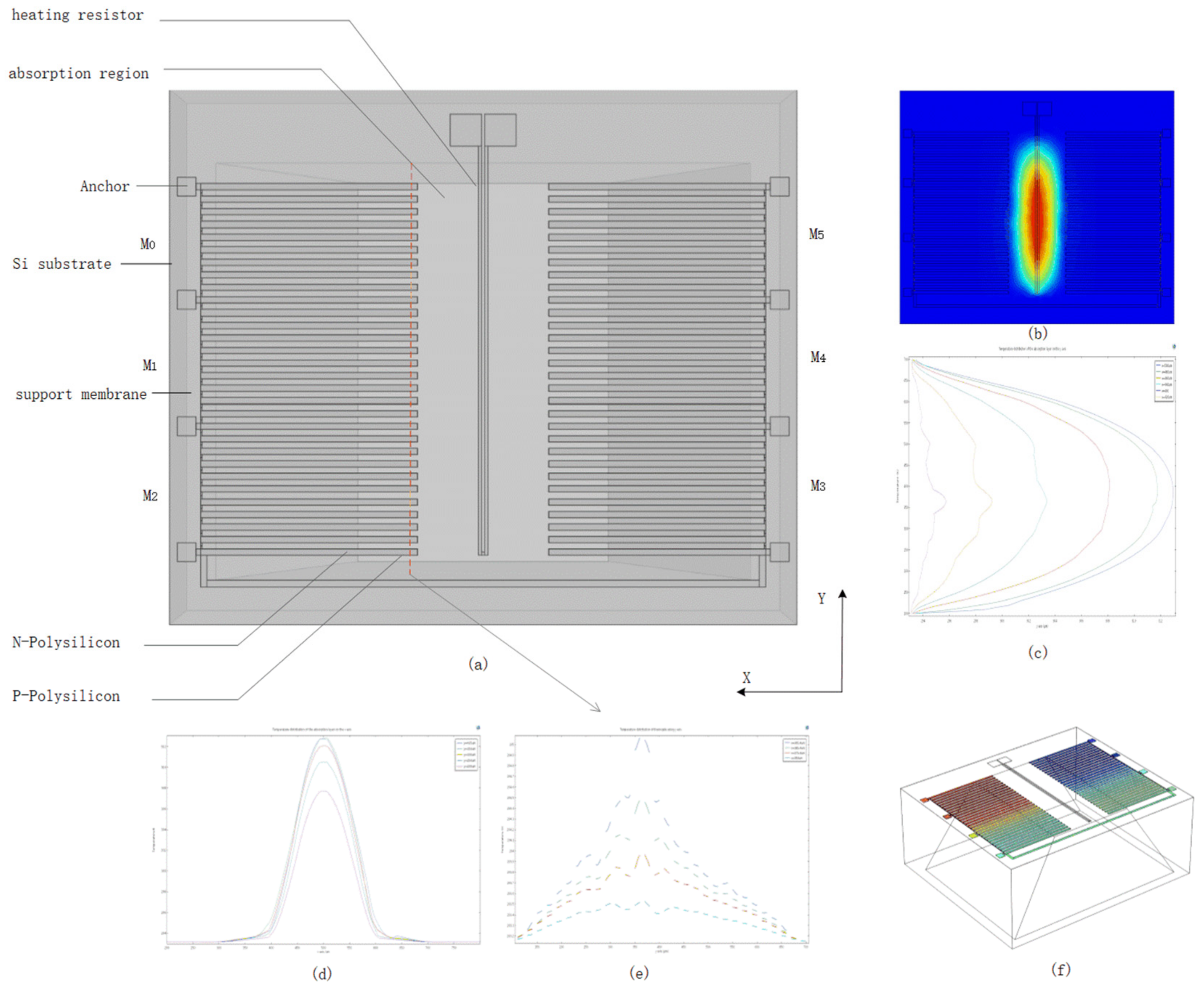
The thermal effect of thermopile with the built-in resistor was analyzed by COMSOL simulation and the results are shown in Figure 4. The simulation conditions are the same as described in Section 2.2. The results indicate that the temperature distribution on the membrane is concentrated in the region where the cavity is located. The overall temperature distribution is axis symmetric along x = 1/2 length of the substrate and y = 1/2 length of the heating resistor as shown in Figure 4d, and the temperature distribution of resistor is shown in Figure 4c, which has a similar to second power relationship with the position of the heating resistor on the y-axis.

3. The Principle of Self-Test, Self-Calibration and Fault Repair

3.1. Self-Test

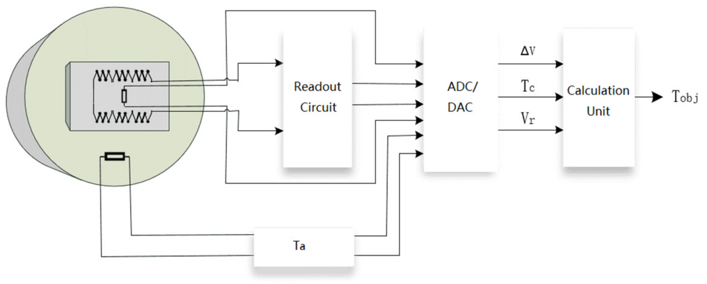
In the self-test mode, the voltage of heating resistor is provided by the digital-to-analog converter (DAC) circuit as shown in Figure 5. The power of the heating resistor is [21]:

$$\mathrm{P}=\mathsf{\epsilon }\frac{V_r{}^2}{r}$$

(14)

$$\mathsf{\epsilon }=\frac{P_{rad}}{P_r}$$

where, $V_r$ is the voltage of heating resistor, $r$is the resistance and $\mathsf{\epsilon }$ is the conversion efficiency of electric power and heat. The responsivity is:

$$\mathrm{R}=\frac{∆V}{P}=\frac{r∆V}{\epsilon V_r{}^2}$$

(15)

The responsivity can be calculated by reading $∆V$ twice with different $V_r$.

$${\delta }_1=\left|R-R_{ref}\right|$$

(16)

$${\delta }_2=\left|R_1-R_2\right|$$

(17)

Under different $V_r$, different responsivities are obtained. According to Equations (16) and (17), we can calculate whether the error is within the allowable range. The use of multiple measurements is mainly due to the low-detection efficiency under a single measurement, which can be explained by the posterior Bayesian probability. It is assumed that the device is detected as a fault as event A, and the device is faulty as event B, then the probability that the detected fault is the actual fault is:

$$\begin{gathered} \mathrm{P}\left(\mathrm{B}|\mathrm{A}\right)=\mathrm{P}\left(\mathrm{B}\right)\frac{P\left(A|B\right)}{P\left(A\right)}=P\left(B\right)\frac{P\left(A|B\right)}{P\left(A|B\right)P\left(B\right)+P\left(A|\overline{B}\right)P\left(\overline{B}\right)} \\ =\frac{1}{1+\frac{p(A|\overline{B})\left(1-P\left(B\right)\right)}{P(A|B)P\left(B\right)}} \end{gathered}$$

(18)

where $\mathrm{P}\left(\mathrm{B}\right)$is the probability of device failure, $\mathrm{P}(\mathrm{A}|\overline{\mathrm{B}})$ is the probability that there is a fault and the device is detected as faulty, $\mathrm{P}(\mathrm{A}|\overline{\mathrm{B}})$ is the probability that there is no failure, but the device is detected as faulty. During fault detection, $\mathrm{P}(\mathrm{A}|\mathrm{B})\gg \mathrm{P}\left(\mathrm{B}\right)\approx \mathrm{P}(\mathrm{A}| \overline{\mathrm{B}} )$, so the Equation (18) can be simplified to:

$$\mathrm{P}\left(\mathrm{B}|\mathrm{A}\right)=\frac{1}{1+\frac{1-\mathrm{P}\left(\mathrm{B}\right)}{\mathrm{P}(\mathrm{A}|\mathrm{B})}}$$

It is not difficult to prove that $\mathrm{P}\left(\mathrm{B}|\mathrm{A}\right)<\mathrm{P}(\mathrm{A}|\mathrm{B})$. Suppose $\mathrm{P}\left(\mathrm{B}\right)=0.1\%, \mathrm{p}\left(\mathrm{B}|\mathrm{A}\right)=99\%, \mathrm{P}\left(\mathrm{A}|\overline{\mathrm{B}}\right)=0.5\%$, and the posterior probability $\mathrm{P}(\mathrm{B}|\mathrm{A})$ is reduced to 19.43%. That it shows a high failure detection rate does not mean high fault detection accuracy. Calculating the responsivity twice under different $V_r$ is an effective means to improve the detection effect.

3.2. Self-Calibration

As already explained in Section 2, a built-in resistor can produce the thermal gradient on the film. Therefore, an equivalent model between the electrical stimulus and physical stimulus needed to be built for the calculation of the right responsivity. The relationship between the absorption power under the two stimuli is defined as follows.

$$P_r=f\left(P_{rad}\right)$$

(19)

where the $P_{rad}$ is the absorption power of infrared radiation, and $P_r$ is the absorption power from the heating resistor. f is the mapping relationship between $P_{rad}$ and $P_r$ which can be fitted by the stimulation of COMSOL in Section 4.

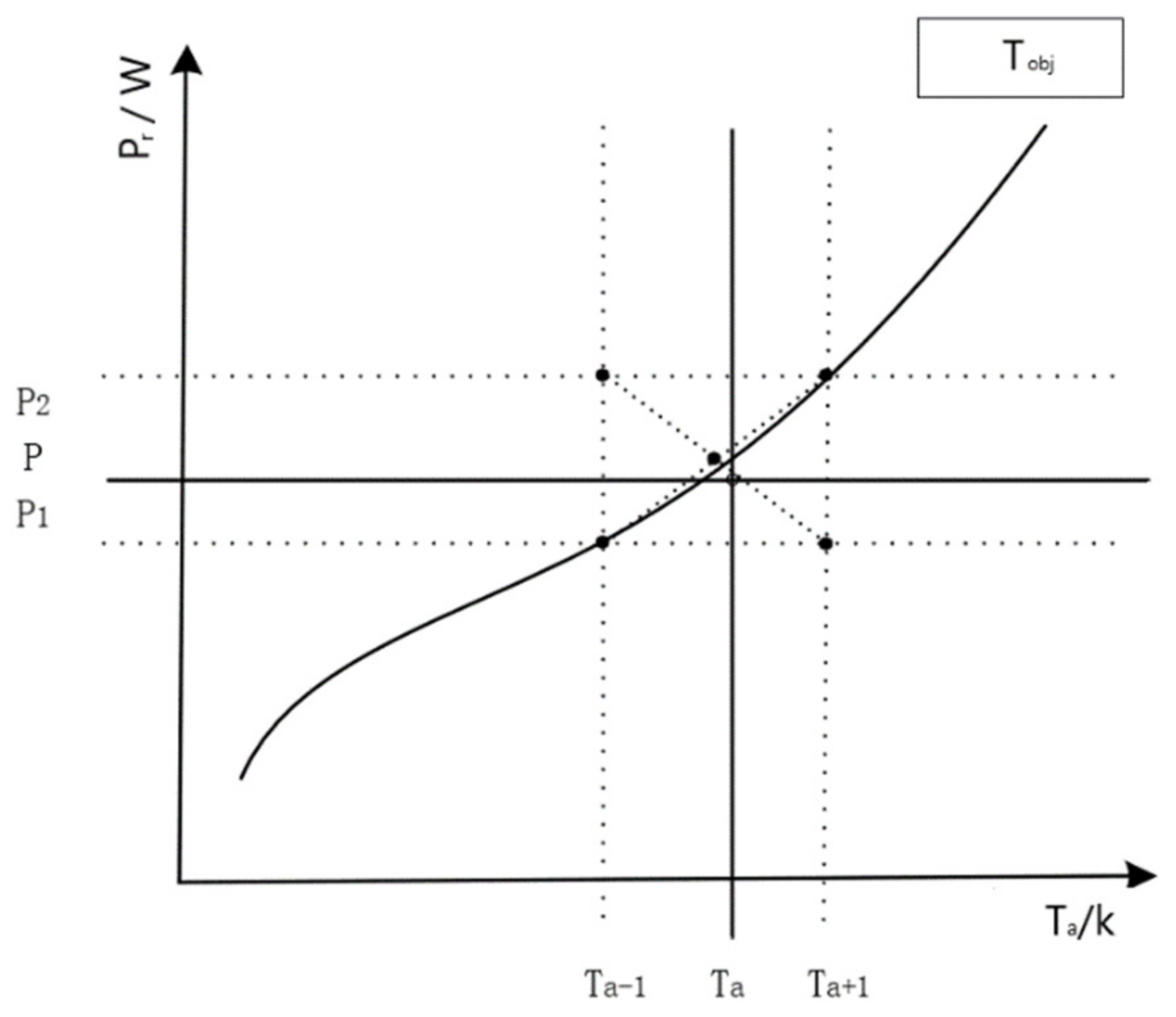
The temperature of object $T_{obj}$ can be calculated by Equation (5). Since the computation is too complex and power consuming, a binary table is used to describe the correspondence relationship between $P_r, T_a$ and $T_{obj}$as shown in Figure 6. The temperature of the object calculated by the equivalent model is:

$$T_{obj}=\sqrt[4]{\frac{f^{-1}\left(P_r\right)}{Ak}+T_a{}^4}$$

(20)

3.3. Fault Analysis and Fault Repair

3.3.1. Analysis of Thermopile Faults and Defects

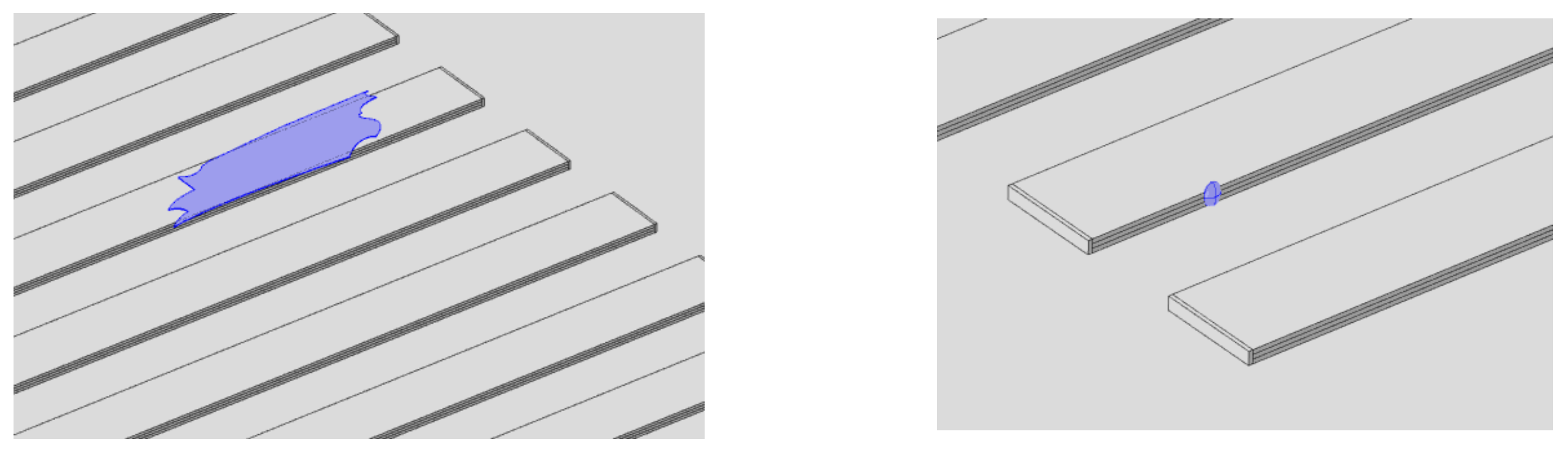
The double-end beam thermopile structure is composed of two materials, N-Polysilicon and P-Polysilicon. This structure can reach a responsivity of 220 V/W in the stimulation. However, the compact structure layout also brings more hidden troubles. Besides, the compact structure of the double-end beam thermopile is more prone to be polluted and adhered to by particles carried with the process of surface cleaning, metal deposition, annealing and packaging, resulting in a short circuit and other defects. Moreover, the thermocouple can be corroded, and the circuit can break because of water vapor and a humid environment. Situations of common corrosion and particle adhesion are shown in Figure 7.

3.3.2. Redundant Repair Yield Model

Suppose a group of defects may occur in N positions of the infrared thermopile detector, that is, there may be N types of defects in the device. Assume that the occurrence of each defect is an independent event, and the probability of each defect occurring is q [22]. The defect described in Section 3.3.1 can thus be expressed as a binomial distribution:

$$P\left(X=x\right)=\left(\begin{array}{c}N\\ x\end{array}\right)q^x{\left(1-q\right)}^{N-x}$$

(21)

Assuming that N is large enough, the binomial distribution evolves into a Poisson distribution, and the average probability of occurrence of defects scattered on the thermopile structure can be obtained.

$$P\left(X=x\right)=\frac{{\lambda }^x}{x!}{e}^{-\lambda }$$

(22)

The distribution estimation by Equation (22) is too pessimistic because of the lack of consideration of the clustering effect, which is the situation where defects occur in the same area. Therefore, the defects distribution function $F\left(x\right)$ can be updated as follows:

$$F\left(x\right)=\frac{1}{\mathsf{\Gamma }\left(k\right){\left(Ab\right)}^{\gamma }}{\lambda }^{\gamma -1}{e}^{-\frac{\lambda }{Ab}}$$

(23)

where A is the area in where the device may have defects, b is the defects density coefficient, $\lambda$ is the average probability of defects, $\mathsf{\gamma }$ is the clustering parameter and $\mathsf{\Gamma }\left(\mathrm{k}\right)$ is the gamma function.

The probability of x defects occurring in the thermopile structure can be expressed as:

$$P\left(x,A\right)=\underset{0}{\overset{x}{{\displaystyle \int }}}\frac{{\lambda }^x}{x!}{e}^{-\lambda }F\left(\lambda \right)d\lambda =\left(\begin{array}{c}x+\gamma -1\\ x\end{array}\right){\left(\frac{Ab}{1+Ab}\right)}^{x}P\left(0,A\right)$$

(24)

The probability of no defect in the detector is:

$$P\left(0,A\right)={\left(\frac{1}{1+Ab}\right)}^{\gamma }$$

(25)

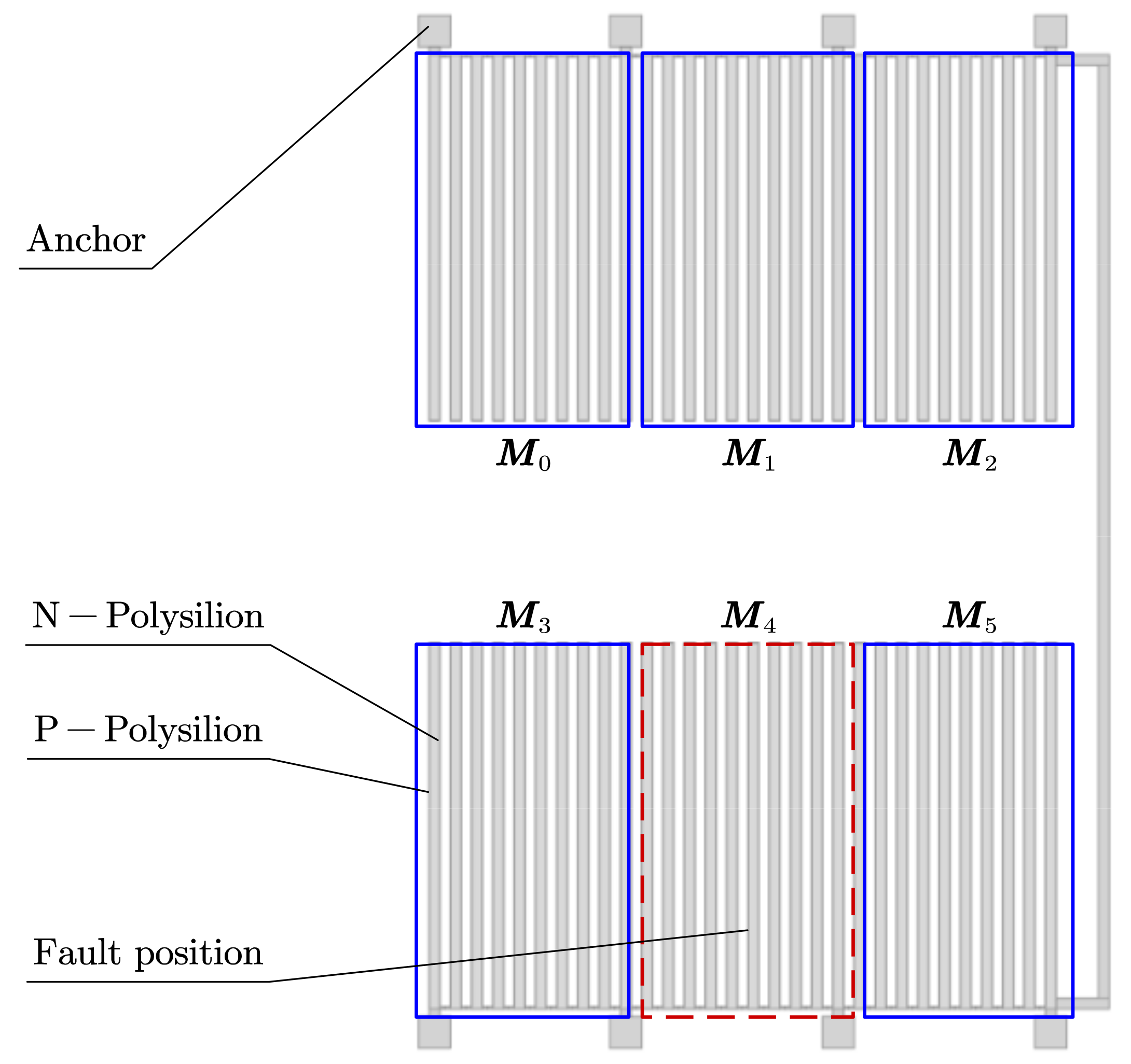
When there is a fault detected by the self-test method, the failure redundancy mechanism will work. According to the above analysis, the thermopile structure can be divided into M modules as shown in Figure 8. The data of the M modules can be read out through time-division multiplexing and the maximum redundant number of M modules is $\mathsf{\zeta }$[23,24]:

$$\mathsf{\zeta }=\frac{1}{2}\times \left(M-1\right)$$

(26)

According to the above analysis, the double-end beam thermopile structure can be divided into 4, 6 and 8 modules, which can tolerate 1, 2, 3 and 4 faults, respectively.

3.3.3. Fault Module Identification

First, fault types of infrared thermopile sensors are discussed according to Section 3.3.1. Faults can be divided into three types: parallel connection of thermocouple, corrosion of thermocouple and disconnection of thermocouple, according to the causes of the defects. There is only a loss for the defects with the parallel connection of thermocouple and corrosion of thermocouple because of the change of thermopile responsivity, but a broken result for disconnection of thermopile defect. Therefore, defects can be classified into parametric defect and catastrophic defect; the former can be corrected by self-calibration and part of the latter can be fixed by self-repair.

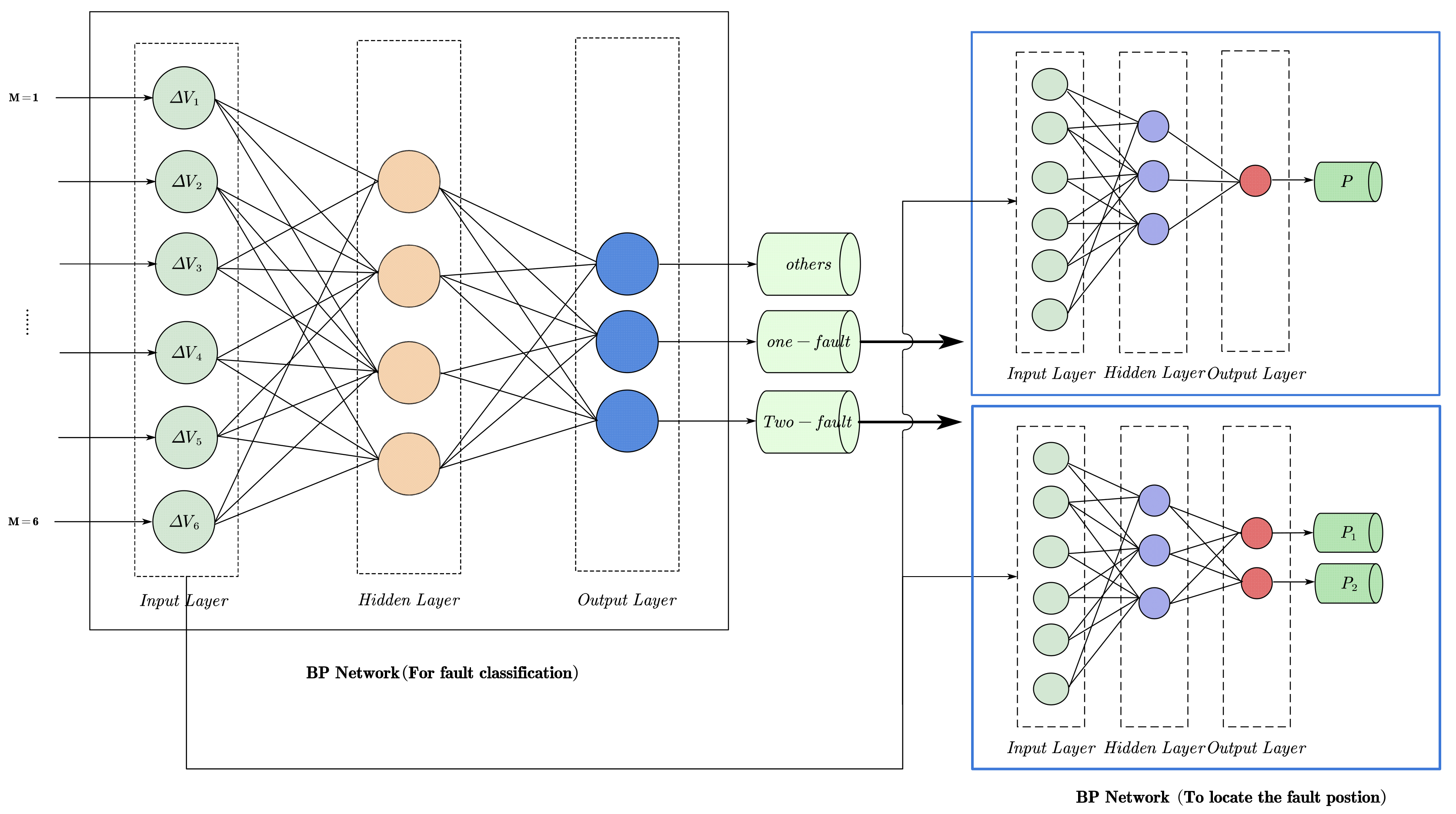
Next, we showed the way to find a fault in M identical modules. The temperature on the composite dielectric film is distributed unevenly, as introduced in the Section 2, which results in different output voltage of each module and makes the fault module identification complicated. To solve this problem a back propagation (BP) neural network is designed and utilized for locating the fault in M identical modules, as shown in Figure 9.

The BP neural network is a multilayer feedforward neural network trained according to the error back propagation algorithm, which can be used for regression and classification problems. In the problem of the M module predicting the fault type and fault location, the BP neural network is used to detect the fault type and fault location. Take the model of M = 6 as an example. The model is divided into two layers of BP network for training. The output of the first layer of BP network is the fault type. Different fault types will choose to enter different second layer BP networks, and there is a total of the types of failures that can be repaired; the second layer of the network is to predict the location of the above-mentioned redundant failure types. Due to the simple data structure, a three-layer network structure is adopted (too many hidden layers will cause the over-fitting phenomenon of the neural network, resulting in insufficient network generalization ability). The hidden layer of the first layer of network is 9, and the hidden layer of the second layer of network is 6, and the activation function selects the sigmoid function.

3.3.4. Recalculate the Responsivity

The location of the fault module can be detected by the BP neural network, then the fault module data is isolated, and the thermopile output voltage is updated:

$$\mathsf{\Delta }{V}^{\prime }={\displaystyle \sum }_{i=1}^M{V}_i, i\ne k\left(k is the position of fault\right)$$

(27)

After fault tolerance, the responsivity calculated according to Equation (3) also needs to be updated. The power absorbed can be calculated as follows.

$$P=A\epsilon \sigma T^4=Ak\left(T_{hot}-T_a\right)T_a{}^3$$

(28)

Therefore, the temperature distribution of the thermopile hot end under different ambient temperatures is fitted by simulation, and the temperature difference ratio of each module is obtained, which is approximated as the M mode power distribution coefficient ${\xi }_m$.

The power $P_r$ can be recalculated by Equation (14), and the responsivity can be updated accordingly.

$$\begin{gathered} {\displaystyle \sum }_{m=1}^M{\xi }_m=1 \\ {P}^{\prime }=\left(1-{\xi }_m\right)P \end{gathered}$$

(29)

4. The Design of Simulation

4.1. Establishment of the Equivalent Model of Electrical Stimulus and Physical Stimulus

To establish an equivalent model between the electrical stimulus and physical stimulus under the same simulation conditions, the response of the thermopile detector under electrical stimulus and physical stimulus was obtained by COMSOL simulation, and then the conversion relationship was fitted by the least-square method. The specific steps are as follows:

(i)

Set the ambient temperature to $T_a=293.15K$ and the heat flux from 0 W/m² to 20,000 W/m², then the relationship between the heat radiation and the output voltage can be obtained;

(ii)

Set the ambient temperature to $T_a=293.15K$ and the voltage of heating resistor from 0 V to 2 V with a step of 0.1, then the relationship between the electrical stimulus and the output voltage can be obtained;

(iii)

Modulate the relationship between the radiation and electric power with the same output voltage.

The relevant simulation parameters are shown in

Table 2. Material parameters of COMSOL simulation.

Attribute and Material Name	Seebeck Coefficient (V/K)	Thermal Conductivity (W/m*K)	Density (Kg/m3)	Heat Capacity at Constant Pressure (J/(Kg*k))	Conductivity (S/m)
Si	−450 × 10−6	131	2329	700	4.7 × 10−4
SiO2	-	1.2	2650	-	0.904
AI	−3.2 × 10−6	237	2700	904	35.5 × 106
N-Polysilicon	−124.17 × 10−6	35	2320	678	-
P-Polysilicon	105.76 × 10−6	30	2320	678	-

and

Table 3. Constructional dimension and technical parameter of thermopile simulation.

Structure Parameter	Dual Ends and Dual Layer Thermopile Structure
N-Polysilicon (L × W × H)	345.4 × 10 × 0.8 μm3
P-Polysilicon (L × W × H)	355.4 × 10 × 0.8 μm3
SiO2 (H)	0.5 μm
Absorbed layer (L × W)	400 × 600 μm2
Number of thermocouples	120
Heater (L × W × H)	650 × 5 × 0.4 μm3

.

4.2. Verification of Fault-Repair and Error Calculation

The prediction of fault type and fault location using the BP neural network described in Section 3.3 is an important step to realize fault repair, and its detection accuracy affects the classification and fault tolerance of faults. Thus, this part verifies the BP neural network’s ability to predict fault types. The neural network training data comes from the COMSOL simulation data. The training output is manually labeled to train the weights of the neural network. Part of the training data is retained as a test set to test the performance of the neural network. The specific verification method is as follows:

(i)

Obtain the fault data set with N defects with simulation, including M modules output data and location of defects;

(ii)

Train the BP neural network with the outputs data of M modules as the inputs and the fault location as the outputs;

(iii)

Calculate the accuracy of the predicted faults under different numbers of modules with the test samples;

(iv)

Calculate the average responsivity error after fault repair with M = 6 modules.

4.3. Calculation Yield

Monte Carlo is a common method to generate random distribution. It is used to simulate the situations of random failures occurring in many MEMS sensor devices which is also used in this paper to simulate the calculation of yield in the production process. The randomly distributed particles constructed on the thermopile structure can be represented as faults by Monte Carlo. The number of particles is generated from 0 to 3, and the particle size is randomly generated from 1 to 10, representing the impact of different types of defects, corresponding to the simulation output data. Defects cause abnormal thermopile output, which can be manifested as no impact, accuracy impact and failure. The corresponding expressions can be catalogued into three types: good, parametric and catastrophic. Figure 10 shows a flowchart of the process of random fault generation with the self-test, self-calibration and fault-repair models accordingly.

5. Result

5.1. Establishment of the Equivalent Model of Electrical Stimulus and Physical Stimulus

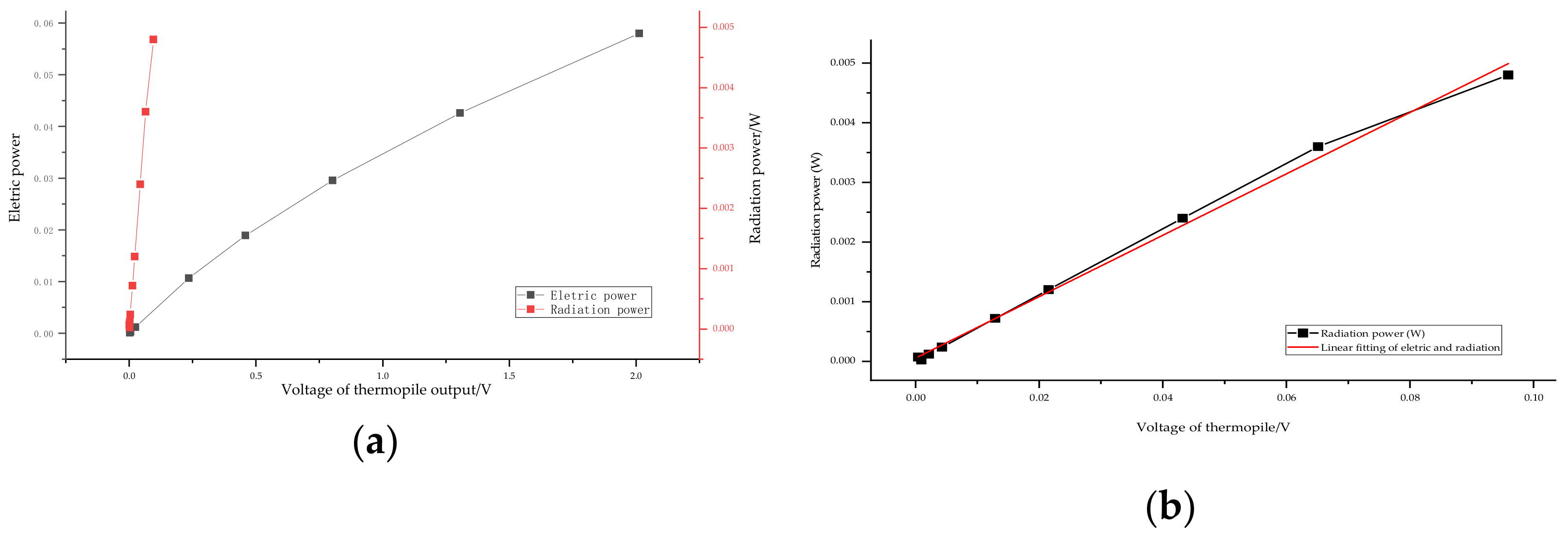
The equivalent model of infrared radiation stimulus and electric stimulus was established by Step 1 of the simulation as introduced in the previous section. As can be seen in Figure 11, the output voltage is linearly related to the electrical stimulus and the radiation stimulus, respectively.

The conversion efficiency of the linear fitting is given in Equation (30). Since the energy transfer by radiation is proportional to the 4th square of temperature, and the energy transfer by heat conduction depends on the temperature gradient.

$$P_{rad}=0.05148P_r+5.4389\times {10}^{-5}$$

(30)

5.2. Prediction Accuracy of Location of Faults and Responsivity Error Calculation

The train data and test data come from the simulation of COMSOL in different failure models, as shown in Figure 6. The BP neural network is trained with the output data of the COMSOL simulation of the thermocouple strip under different assumptions such as corrosion, short circuit, open circuit, etc., and then, the trained BP network can be used to predict the fault location.

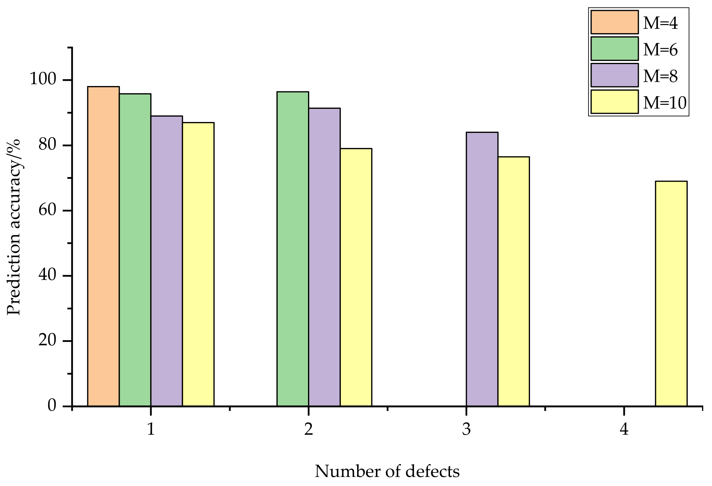
The results, as shown in Figure 12, indicate that predictive ability decreases as the number of failures increases. It indicates that for the M modules’ redundancy, the fault location is easier to identify with fewer faults, and the predictions are more accurate. The fewer modules of M, the higher the recognition rate is. In addition, the larger M is, the more abundant samples are needed, and the number of hidden layer units required by the neural network increases, so the cost will also increase accordingly.

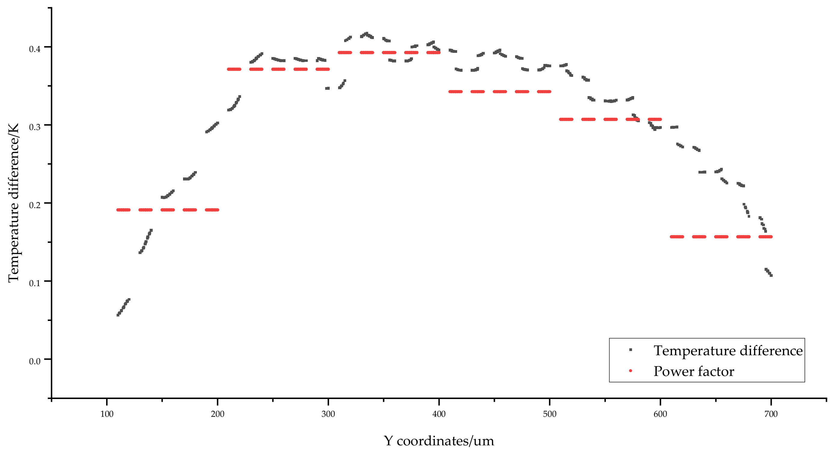
The fault-repair model of the thermopile structure can be divided into six modules with high accuracy and appropriate cost. The average temperature distribution of the hot end of the thermopile under different ambient temperatures in M = 6 is shown in Figure 13. Furthermore, the electric power weight values with each module number can be seen in

Table 4. Electric power proportion ${\xi }_m$ and its calculated responsivity error.

Position	1	2	3	4	5	6
Weights	0.1085	0.2108	0.2229	0.1945	0.1744	0.0889
Error	−0.0357	0.0637	−0.0853	−0.0547	0.1153	−0.00233

, which can be used to recalculate the responsivity with fault repair. The responsivity error calculated in Table 4 is the average error of a single fault under different modules. The total average error is $9.7\times {10}^{-4}$and the mean square error is 0.0694. The above results verify that the error caused by the fault-repair model has little effect on the accuracy of the responsivity.

5.3. Faults Simulation by Monte Carlo and Yield Calculation

With the fault dataset obtained by the Monte Carlo method, the self-test, self-calibration and fault-repair were conducted according to the process as shown in Figure 10, and then the simulation results were obtained and are given in

Table 5. Self-test, self-calibration and fault-repair models before and after yield.

The Number of Defects	1	2	3	4	5	6
Good	770	616	501	396	320	273
Parametric	63	14	4	4	0	1
Catastrophic	167	370	495	600	680	726
Yield (before)	77%	61.6%	50.1%	39.6%	32%	27.3%
Yield (after)	89.1%	73.4%	58.8%	45.7%	34.1%	27.4%

. It can be seen from Table 5 that in mass production, the greater the number of defects is, the greater the possibility that the devices will fail. The yield can be improved with the self-test, self-calibration and fault-repair processes, especially when there are more parametric defects. However, there is a limit to how much yield can be achieved when there are too many catastrophic defects, since only part of catastrophic defects can be repaired. Therefore, there is a significant correlation between the improved yield and the defect types and numbers. On the other hand, with the increase of the number of defects, the neural network recognition accuracy decreases, which is negative for the yield improving. Overall, these results show the effectiveness of the self-test, self-calibration and fault-repair models.

6. Conclusions

In this article, to enhance reliability and high yield, a novel MEMS infrared thermopile detector construction is designed that builds in a heating resistor on the membrane central and partitions the thermopile into M identical modules. The establishment of both an equivalent model of the electrical stimulus and physical stimulus and a faults analysis model based on M identical modules is fundamental to achieve the self-test, self-calibration and self-repair in this issue. Based on that, the major work is to build an effective model to achieve test, calibration and repair for faults on chip, and finally to imply the improvement of reliability and high yield for detectors. Therefore, a dual standard suggested for the self-test is to have an equivalent model and lookup table used to achieve the calibration and a redundant and fault-tolerant mechanism designed for fault repair with M identical modules when detector fails the test. To verify the validity of the model, the Monte Carlo method was used to simulate the fault output model generated by random defects, and the proposed model was used to process the detectors data. The results suggest that when the number of thermopile modules M = 6, the model has excellent prediction accuracy and an appropriate cost. And the comparison of the findings with different number of defects indicates the improvement of the yield dependent on the proportion of fault types. In summary, these results show the proposed model has an effective improvement in yield. Overall, this paper provides a wide insight into design for testability in combination with a self-test, self-calibration and self-repair model which is significative for future works.

References

- Du, H.; Bogue, R. MEMS sensors: Past, present and future. Sensor Rev. 2007, 27, 7–13. [Google Scholar]
- Huo, D.; Zhap, J.; Guo, F. Research on the current status and development direction of MEMS sensor reliability technology in smart home based on the IOT. Internet Things Technol. 2018, 8, 37–39. [Google Scholar]
- Brigante, C.M.N.; Abbate, N.; Basile, A.; Faulisi, A.C.; Sessa, S. Towards Miniaturization of a MEMS-Based Wearable Motion Capture System. IEEE Trans. Ind. Electron. 2011, 58, 3234–3241. [Google Scholar] [CrossRef]
- Li, D.; Huang, M.; Zhao, C.; Gong, Y.; Zhang, Y. Construction of 5G smart Medical Service System for COVID-19 prevention and control. Chin. J. Emerg. Med. 2020, 29, 503–508. [Google Scholar]
- Lu, J.; Wei, S. Successful development of infrared thermometer calibration device—The Chinese Academy of Metrology has made new achievements in combating SARS. China Metrol. 2003, 6, 6–7. [Google Scholar]
- Hartzell, A.L.; da Silva, M.G.; Shea, H.R. MEMS Reliability; Springer Science and Business Media LLC: New York, NY, USA, 2011. [Google Scholar] [CrossRef]
- Sviridova, T.; Kushnir, Y.; Korpyljov, D. An Overview of MEMS Testing Technologies. In Proceedings of the International Conference on Perspective Technologies & Methods in Mems Design, Lviv, Ukraine, 24–27 May 2006. [Google Scholar]
- Rosing, R.; Richardson, A.; Dorey, A. Peyton. A. Test support Strategies for MEMS. Des. Charrette 1999. [Google Scholar] [CrossRef]
- Jiakai, L.; Xinglin, Q.I.; Xiaofang, W.; Long, X. Reliability Enhancement Test Technology of Fuze MEMS Mechanism. J. Detect. Control 2013, 35, 41–45. [Google Scholar]
- Lee, S.W. Development of a MEMS fabrication process for self-assembly of on-chip antennas. Ph.D. Thesis, Simon Fraser University, Burnaby, BC, Canada, May 2012. [Google Scholar]
- Liu, C.; Fu, J.; Hou, Y.; Zhou, Q.; Chen, D.P. A Self-Calibration Method of Microbolometer With Vacuum Package. IEEE Sens. 2020, 20, 8570–8575. [Google Scholar] [CrossRef]
- Wang, K.J. Design and Characteristic Measurement of a Thermopile Infrared Detector. Master’s Thesis, North University of China, Taiyuan, China, 2010. [Google Scholar]
- Lei, C. Research on the Key Technologies of Double-end-beam based MEMS Thermopile IR Detector. Ph.D. Thesis, North University of China, Taiyuan, China, 2016. [Google Scholar]
- Wang, L.T.; Wu, C.W.; Wen, X. VLSI Test Principles and Architecture Design for Testability; Morgan Kaufmann: Amsterdam, The Netherlands, 2006; p. 808. ISBN 978-0-12-370597-6. [Google Scholar] [CrossRef]
- Charlot, B.; Mir, S.; Parrain, F. Generation of Electrically Induced Stimuli for MEMS Self-Test. J. Electron. Test. Theory Appl. 2001, 17, 459–470. [Google Scholar] [CrossRef]
- Rekik, A.A.; Azas, F.; Mailly, F.; Nouet, P.; Masmoudi, M. Self-test and self-calibration of a MEMS convective accelerometer. In Proceedings of the 2013 Symposium on Design, Test, Integration and Packaging of MEMS/MOEMS (DTIP), Barcelona, Spain, 16–18 April 2013; pp. 1–4. [Google Scholar]
- Ozel, M.K.; Cheperak, M.; Dar, T.; Kiaei, S.; Bakkaloglu, B.; Ozev, S. Electrical-Stimulus-Only BIST IC for Capacitive MEMS Accelerometer Sensitivity Characterization. Sensors 2017, 17, 695–708. [Google Scholar] [CrossRef] [Green Version]
- Li, J.; Huang, Z.; Wang, W. Built-In Self-Calibration of CMOS-Compatible Thermopile Sensor with On-Chip Electrical Stimulus. In Proceedings of the IEEE European Test Symposium, Paderbron, Germany, 26–30 May 2014; pp. 1–6. [Google Scholar]
- Kuan, H.; Weibing, W.; Jia, L. Self-calibration response analysis of MEMS infrared thermopile based on neural network. Microcomput. Appl. 2017, 36, 48–50. [Google Scholar]
- Hou, Z. Thermal Conductivity of Solid; Shanghai Scientific & Technical Publishers: Shanghai, China, 1984. [Google Scholar]
- Meinel, W.B.; Lazarov, K.V. On-chip calibration system and method for infrared sensor. U.S. Patent Application 20120138800, 14 February 2014. [Google Scholar]
- Hirase, J. Yield increase of VLSI after redundancy-repairing. In Proceedings of the Asian Test Symposium IEEE, Kyoto, Japan, 19–21 November 2001. [Google Scholar]
- Hao, S.Y.; Yang, Z.; Chai, Z.Q. Study on Memory’s Fault tolerant Design based on Multiple Module Redundancy Reconfiguration. Comput. Meas. Control China 2009, 17, 190–191. [Google Scholar]
- Koren, I.; Su, S. Reliability Analysis of N-Modular Redundancy Systems with Intermittent and Permanent Faults. IEEE Trans. Comput. 1979, 28, 514–520. [Google Scholar] [CrossRef]
Figure 1.
Diagram of the Seebeck effect.
Figure 2.
The closed-mode structure of infrared thermopile detector in this paper.
Figure 3.
Temperature gradient on membrane by (a) physical stimulus and (b) electrical stimulus.
Figure 4.
(a) Thermopile structure with self-test, self-calibration and self-repair functions proposed in this paper. (b) Temperature distribution map of the absorption layer stimulated by built-in heating resistor. (c) Temperature distribution of the absorption layer along the y-axis. (d) Temperature distribution of the absorption layer along the x-axis. (e) Thermopile temperature distribution along the x-axis. (f) The electric potential stimulated distribution on the thermopile. (A clearer version in Supplementary Materials).
Figure 5.
Self-test model of infrared thermopile detector.
Figure 6.
Binary lookup table of target object temperature (inputs are , ).
Figure 7.
Schematic diagram of thermopile metal corrosion and particle adhesion.
Figure 8.
M modules of thermopile (M = 6).
Figure 9.
BP Neural network structure diagram.
Figure 10.
Flowchart of self-test, self-calibration and fault-repair model.
Figure 11.
(a)The relationship between infrared radiation power, heating resistance power and output voltage. (b) Linear fitting function of electric and radiation stimuli.
Figure 12.
M module prediction responsivity.
Figure 13.
Temperature distribution at the hot end of the thermopile (M = 6).