The Problem of the Non-Uniqueness of the Solution to the Inverse Problem of Recovering the Symmetric States of a Bistable Medium with Data on the Position of an Autowave Front

Abstract

The paper considers the question of the possibility of recovering symmetric stable states of a bistable medium in the inverse problem for a nonlinear singularly perturbed autowave equation by data given on the position of an autowave front propagating through it. It is shown that under certain conditions, this statement of the problem is ill-posed in the sense of the non-uniqueness of the solution. A regularizing approach to its solution was proposed.

1. Introduction

Problems for nonlinear singularly perturbed autowave equations arise when simulating propagating fronts of various natures. Such problems include for example flame propagation modeling in combustion theory [1] or the problem of population habitat movement in biophysics [2]. The unknown function in the direct problem is the density of a combustible substance or the size of a population. Usually, mathematical models describing these processes include differential equations with cubic nonlinearities. With the help of such nonlinearities, it is possible to describe physical systems that have two equilibrium states and the autowave front that matches state switching. The equilibrium states are related to the maximal and minimal roots of the cubic nonlinearity [2]. The front is a region where the function of matter density (in the case of chemical kinetics) or population size (in the case of biophysical problems) changes quite sharply from values close to one root of the cubic nonlinearity to values close to another root. In this case, space is divided into two media: the disturbed part, through which the front has already passed, and the unperturbed part. If a small parameter is placed at the highest derivative, the width of the switching autowave front will be rather small compared to the entire region size [3]. As a consequence, the front can be distinguished experimentally.

If the medium root of the cubic nonlinearity at each point of the area is equal to the half-sum of the other two roots (which are called symmetric stable states of a bistable medium), then such nonlinearity is called balanced nonlinearity [4,5]. Problem statements with balanced nonlinearities describe physical quantities taking values corresponding to one of two stationary states, symmetric with respect to an unstable neutral equilibrium position. Such values can be, for example, the number of fixed and disappearing mutations in the model describing the autowave front of mutations passing through the population [6,7].

Some applied problem statements in these models require solving inverse problems for recovering some coefficient in the equation. To formulate the inverse problem, additional information is required, which is usually measured experimentally. Often in the statements of inverse problems for partial differential equations, additional information about the solution on a part of the boundary is used (see, for example, [8,9,10,11,12,13,14,15,16,17]). In particular, in [18,19], the authors considered the features of the numerical solution of the inverse problems for nonlinear singularly perturbed partial differential equations with data at the final moment of time. However, one of the possible inverse problem statements for equations of this type is a statement with additional information on front motion dynamics (see, for example, [20,21]). Additional data of this type is demanded in practice since they are the easiest to observe in the experiment (the front is an easily distinguishable contrast structure). In this paper, we considered the possibility of recovering the unknown function describing the stable state of a bistable medium from the data on the moving autowave front position.

The main idea that can be applied to effectively solve the inverse problem under consideration is the use of asymptotic analysis methods [22,23]. The application of the asymptotic analysis methods to nonlinear differential equations with a small parameter at the highest derivative has an important feature. This feature is that the asymptotic analysis under certain conditions makes it possible to reduce the original problem for a nonlinear singularly perturbed partial differential equation to a much simpler problem. Such a problem does not contain small parameters and has a lower dimension (and sometimes does not even contain differential, but algebraic equations). As a result of applying this approach, it is possible to obtain a reduced formulation of the inverse problem. In this formulation, the coefficient in the equation (stable state of a bistable medium) is explicitly related to the position of the moving autowave front that is observed experimentally.

Similar ideas allowing obtaining a simpler relationship between the coefficients of the equation and the position of the front have been proposed earlier. For example, in [1,3], the question of determining the approximate value of the front velocity for singularly perturbed partial differential equations of the type under consideration was studied. However, in the case of balanced nonlinearity, the methods from [1,3] give an approximate value of the front speed identically equal to zero, which does not correspond to reality. The use of asymptotic analysis methods [22,23] makes it possible to refine the expression for the velocity, which in the next approximation will be nonzero.

The structure of this work is as follows. Section 2 contains the inverse problem statement for recovering the coefficient that determines the symmetric states of a bistable medium from data on the autowave front position. In Section 3, as a result of the direct problem’s asymptotic analysis, a reduced formulation of the problem is derived that explicitly relates the unknown coefficient with the data of the inverse problem. In Section 4, using this reduced formulation of the inverse problem, we demonstrate the fact that the original inverse problem under certain conditions has a non-unique solution. One of the possible regularizing approaches to solve this problem was proposed.

2. Statement of the Inverse Problem

Consider the following direct problem for a nonlinear singularly perturbed equation with a balanced cubic nonlinearity:

$$\left\{\begin{array}{c}{\epsilon }^2\left(\frac{{\partial }^{2}u}{\partial x^2}-\frac{\partial u}{\partial t}\right)=u\left(u^2-q^2\left(x\right)\right),x\in (0,1),t\in (0,T],\hfill \\ u(0,t)=u_{left}\left(t\right),u(1,t)=u_{right}\left(t\right),t\in (0,T],\hfill \\ u(x,0)=u_{init}\left(x\right),x\in [0,1],\hfill \end{array}\right.$$

(1)

where $0<\epsilon \ll 1$ is a small parameter and the functions $u_{left}\left(t\right)$, $u_{right}\left(t\right)$, $u_{init}\left(x\right)$, and $q\left(x\right)$ are sufficiently smooth.

It is known [4] that under certain conditions, the problem (1) has a solution in the form of a moving front, i.e., the solution of the problem is close to the functions $-q\left(x\right)$ and $+q\left(x\right)$ to the left and to the right of some point $x_{t.p.}\left(t\right)$, and in a small neighborhood of this point, a narrow internal transition layer is observed (see Figure 1). We call the point $x_{t.p.}\left(t\right)$ a “transition point” (“t.p”).

The function $x=x_{t.p.}\left(t\right)$, describing the position of the front, according to [23], can be found as a solution to the following functional equation (see Figure 1):

$$u(x,t)=0,t\in [0,T].$$

Thus, we can match the coefficient $q\left(x\right)$ determining the stable state of a bistable medium in the problem (1), which has a solution of the moving front type, with the position of this front $x_{t.p.}\left(t\right)\equiv f\left(t\right)$ at any time $t\in [0,T]$ (see Figure 1).

The inverse problemis to determine the coefficient $q\left(x\right)>0$ in (1) from the known additional information about the position of the front:

$$x_{t.p.}\left(t\right)=f\left(t\right),t\in [0,T].$$

(2)

Note that in practice, instead of the exact data $f\left(t\right)$, the experimentally measured approximate value $f_{\delta }\left(t\right)$ is known, such that:

$$\parallel f-f_{\delta }{\parallel }_{L_2}\le \delta .$$

3. Construction of the Reduced Statement of the Inverse Problem Using the Asymptotic Analysis Methods

Asymptotic analysis (see, for example, [22,23,24]) allows determining approximately the theoretical law of motion of the front localization point $x_{t.p}$. According to asymptotic analysis methods, it is assumed that for the solution $u(x,t)$ of the problem (1), the position of point $x_{t.p}\left(t\right)$ at each moment of time is determined by the equality $u\left(x_{t.p.}\left(t\right),t\right)=0$, $t\in [0,T]$. In order to obtain the function $x_{t.p.}\left(t\right)$, we constructed the function $U(x,t)$, which is an asymptotic approximation of $u(x,t)$ with respect to the small parameter $\epsilon$. We constructed $U(x,t)$ separately on each of the segments $x\in [0,x_{t.p.}\left(t\right)]$ and $x\in [x_{t.p.}\left(t\right),1]$ at each moment of time $t\in [0,T]$. Further, the functions defined on the segment $[0,x_{t.p.}\left(t\right)]$ are denoted by the superscript “$(-)$”, and on the segment $[x_{t.p.}\left(t\right),1]$ by the superscript “$(+)$”.

Let us write the asymptotic approximation $U(x,t)$ of the problem (1) solution on each of the indicated intervals as a sum of three terms:

$$U^{(\mp )}(x,t)={\overline{u}}^{(\mp )}\left(x\right)+Q^{(\mp )}(\xi ,t)+{\Pi }^{(\mp )}\left({\rho }_{\mp }\right).$$

(3)

Here:

• ${\overline{u}}^{(\mp )}\left(x\right)$ are the regular part functions describing the behavior of the solution far from the points $x\in \{0,x_{t.p.}\left(t\right),1\}$;
• $Q^{(\mp )}(\xi ,t)$ are the transition layer functions describing the solution near the localization point $x_{t.p}\left(t\right)$ of the transition layer at each time and depending on the stretched variable $\xi =(x-x_{t.p.}\left(t\right))/\epsilon$;
• ${\Pi }^{(-)}\left({\rho }_{-}\right)$ is a boundary function describing the solution near the point $x=0$ and depending on the stretched variable ${\rho }_{-}=x/\epsilon$;
• ${\Pi }^{(+)}\left({\rho }_{+}\right)$ is a boundary function describing the behavior of the solution near the point $x=1$ and depending on the stretched variable ${\rho }_{+}=(x-1)/\epsilon$; note that the boundary functions exponentially decrease with distance from the points $x=0$ and $x=1$ [24].

Let us represent the functions included in sums (3) as small parameter exponents:

$$\begin{array}{cc}\hfill & {\overline{u}}^{(\mp )}\left(x\right)={\overline{u}}_0^{(\mp )}\left(x\right)+\epsilon {\overline{u}}_1^{(\mp )}\left(x\right)+{\epsilon }^2{\overline{u}}_2^{(\mp )}\left(x\right)+\dots ,\hfill \\ \hfill & Q^{(\mp )}(\xi ,t)=Q_0^{(\mp )}(\xi ,t)+\epsilon Q_1^{(\mp )}(\xi ,t)+{\epsilon }^2{Q}_2^{(\mp )}(\xi ,t)+\dots ,\hfill \\ \hfill & {\Pi }^{(\mp )}\left({\rho }_{\mp }\right)={\Pi }_0^{(\mp )}\left({\rho }_{\mp }\right)+\epsilon {\Pi }_1^{(\mp )}\left({\rho }_{\mp }\right)+{\epsilon }^2{\Pi }_2^{(\mp )}\left({\rho }_{\mp }\right)+\dots .\hfill \end{array}$$

(4)

If sums (4) contain terms up to the order ${\epsilon }^n$, then the corresponding approximations for $U(x,t)$ are denoted with the subscript n and called the asymptotic approximations of the n-th order.

According to [22,23,24], the functions $U_n^{(-)}(x,t)$ and $U_n^{(+)}(x,t)$ are subject to the condition of equality at the point $x_{t.p.}\left(t\right)$ at each moment of time $t\in [0,T]$:

$$\begin{array}{cc}\hfill & U_n^{(-)}\left(x_{t.p.}\left(t\right),t\right)=\sum _{i=0}^n{\epsilon }^i\left({\overline{u}}_i^{(-)}\left(x_{t.p.}\left(t\right)\right)+Q_i^{(-)}(0,t)\right)+O\left({\epsilon }^{n+1}\right)=\hfill \\ \hfill & =U_n^{(+)}\left(x_{t.p.}\left(t\right),t\right)=\sum _{i=0}^n{\epsilon }^i\left({\overline{u}}_i^{(+)}\left(x_{t.p.}\left(t\right)\right)+Q_i^{(+)}(0,t)\right)+O\left({\epsilon }^{n+1}\right).\hfill \end{array}$$

(5)

Taking into account the equality $u\left(x_{t.p.}\left(t\right),t\right)=0$, we have $U_n^{(-)}\left(x_{t.p.}\left(t\right),t\right)=0$ and $U_n^{(+)}\left(x_{t.p.}\left(t\right),t\right)=0$.

Note that due to the exponential decay of the boundary functions ${\Pi }^{(\mp )}$ with distance from the endpoints of the segment $[0,1]$ their contribution to the matching conditions of the functions $U_n^{(-)}(x,t)$ and $U_n^{(+)}(x,t)$ is of order less than $O\left({\epsilon }^{n+1}\right)$ in case the transition layer is far enough from the points $x=0$ and $x=1$.

We assumed that the function $x_{t.p.}\left(t\right)$ can also be represented with exponents of the small parameter $\epsilon$:

$$x_{t.p.}\left(t\right)=x_0\left(t\right)+\epsilon x_1\left(t\right)+\dots +{\epsilon }^n{x}_n\left(t\right)+\dots$$

(6)

According to the standard methods of asymptotic analysis [23] the coefficients $x_i\left(t\right)$, $i=\overline{0,n}$, in sums (6) are determined sequentially from the conditions for matching the derivatives of the asymptotic approximations of the i-th order $U_i^{(-)}(x,t)$ and $U_i^{(+)}(x,t)$, $i=\overline{0,n}$, at the point $x_{t.p.}\left(t\right)$ for each $t\in (0,T]$.

We remind that in the current work, Equation (1) with balanced nonlinearity [4,5] is considered. In this case, the coefficient $x_0\left(t\right)$ of the expansion (6) is determined from the condition of matching the derivatives with respect to the variable x of the first-order asymptotic approximations $U_1^{(-)}(x,t)$ and $U_1^{(+)}(x,t)$ at the point $x_{t.p.}\left(t\right)$ for all $t\in [0,T]$.

According to Vasilyeva’s algorithm [23], the equations for the functions of the regular part ${\overline{u}}_i^{(\mp )}\left(x\right),$$i=0,1$, are obtained from the equalities:

$$O\left({\epsilon }^2\right)=\left({\overline{u}}_0^{(\mp )}+\epsilon {\overline{u}}_1^{(\mp )}\right)\left({\left({\overline{u}}_0^{(\mp )}+\epsilon {\overline{u}}_1^{(\mp )}\right)}^2-q^2\left(x\right)\right),$$

if we equate the coefficients for ${\epsilon }^0$ and ${\epsilon }^1$, respectively, in the Taylor series expansion over the small parameter $\epsilon$ of the left and right parts of these equalities.

Thus, we obtain the equations to define the functions ${\overline{u}}_0^{(\mp )}\left(x\right)$:

$${\overline{u}}_0^{(\mp )}\left({\left({\overline{u}}_0^{(\mp )}\right)}^2-q^2\left(x\right)\right)=0.$$

Each of these equations has three roots: $\{0,\pm q(x\left)\right\}$. As is known from [23], to construct an asymptotic approximation of an increasing solution of the front form, one should set:

$${\overline{u}}_0^{(-)}=-q\left(x\right),{\overline{u}}_0^{(+)}=q\left(x\right).$$

For the functions of the regular part of the first order in the mentioned way, we obtained the equations, from which it follows that:

$${\overline{u}}_1^{(\mp )}\equiv 0.$$

The equations for the transition layer functions were obtained in the same way as for the regular part, from the equalities:

$$\begin{array}{cc}\hfill & {\epsilon }^2\frac{{\partial }^2}{\partial x^2}\left({\overline{u}}_0^{(\mp )}(x_{t.p.}+\epsilon \xi )+\epsilon {\overline{u}}_1^{(\mp )}(x_{t.p.}+\epsilon \xi )\right)+{\displaystyle \frac{{\partial }^2}{\partial {\xi }^2}}\left(Q_0^{(\mp )}+\epsilon Q_1^{(\mp )}\right)+\hfill \\ \hfill & +\epsilon \frac{d{x}_{t.p.}}{dt}{\displaystyle \frac{\partial }{\partial \xi }}\left(Q_0^{(\mp )}+\epsilon Q_1^{(\mp )}\right)=\hfill \\ \hfill & =\left({\overline{u}}_0^{(\mp )}(x_{t.p.}+\epsilon \xi )+\epsilon {\overline{u}}_1^{(\mp )}(x_{t.p.}+\epsilon \xi )+Q_0^{(\mp )}+\epsilon Q_1^{(\mp )}\right)\times \hfill \\ \hfill & \times \left({\left({\overline{u}}_0^{(\mp )}(x_{t.p.}+\epsilon \xi )+\epsilon {\overline{u}}_1^{(\mp )}(x_{t.p.}+\epsilon \xi )+Q_0^{(\mp )}+\epsilon Q_1^{(\mp )}\right)}^2-q^2(x_{t.p.}+\epsilon \xi )\right)-\hfill \\ \hfill & -\left({\overline{u}}_0^{(\mp )}(x_{t.p.}+\epsilon \xi )+\epsilon {\overline{u}}_1^{(\mp )}(x_{t.p.}+\epsilon \xi )\right)\times \hfill \\ \hfill & \times \left({\left({\overline{u}}_0^{(\mp )}(x_{t.p.}+\epsilon \xi )+\epsilon {\overline{u}}_1^{(\mp )}(x_{t.p.}+\epsilon \xi )\right)}^2-q^2(x_{t.p.}+\epsilon \xi )\right)+O\left({\epsilon }^2\right).\hfill \end{array}$$

(7)

In the last equality, the argument t of function $x_{t.p.}\left(T\right)$ is omitted for brevity.

The functions $Q_i^{(-)}(\xi ,t)$, $i=\{0,1\}$, are defined on the half-line $\xi \le 0$ and the functions $Q_i^{(+)}(\xi ,t)$ on the half-line $\xi \ge 0.$ The boundary conditions for $\xi =0$ for these functions are obtained from the equalities (5).

We also require the standard condition for decreasing at infinity [23]:

$$Q_i^{(\mp )}(\mp \infty ,t)=0.$$

(8)

We denote:

$$\tilde{u}(\xi ,t)=\left\{\begin{array}{cc}{\overline{u}}_0^{(-)}\left(x_{t.p.}\left(t\right)\right)+Q_0^{(-)}(\xi ,t),\hfill & \hfill \xi \in (-\infty ,0],t\in [0,T],\\ {\overline{u}}_0^{(+)}\left(x_{t.p.}\left(t\right)\right)+Q_0^{(+)}(\xi ,t),\hfill & \hfill \xi \in [0,+\infty ),t\in [0,T].\end{array}\right.$$

Note that this function is defined for $\xi \in (-\infty ,+\infty )$ and is continuous due to the condition (5) in order ${\epsilon }^0.$

Combining the terms for ${\epsilon }^0$ in the equalities (7) and (5), taking into account the conditions at infinity (8), for the function $\tilde{u}(\xi ,t)$, we obtain a problem where t is a parameter:

$$\left\{\begin{array}{c}{\displaystyle \frac{{\partial }^2\tilde{u}}{\partial {\xi }^2}}=\tilde{u}\left({\tilde{u}}^2-q{\left(x_{t.p.}\left(t\right)\right)}^2\right),\xi \in (-\infty ,+\infty ),\hfill \\ \tilde{u}(-\infty ,t)=-q\left(x_{t.p.}\left(t\right)\right),\tilde{u}(+\infty ,t)=q\left(x_{t.p.}\left(t\right)\right).\hfill \end{array}\right.$$

(9)

It is known [25] that this problem has a smooth solution. Let us pass from the second-order differential equation in (9) to the equivalent system:

$$\left\{\begin{array}{c}\Phi ={\displaystyle \frac{\partial \tilde{u}}{\partial \xi }},\hfill \\ {\displaystyle \frac{\partial \Phi }{\partial \xi }}=\tilde{u}\left({\tilde{u}}^2-q{\left(x_{t.p.}\left(t\right)\right)}^2\right),-\infty <\xi <+\infty ,\hfill \end{array}\right.$$

(10)

and from it to the equation for phase trajectories on the plane $(\tilde{u},\Phi )$:

$$\Phi {\displaystyle \frac{\partial \Phi }{\partial \tilde{u}}}=\tilde{u}\left({\tilde{u}}^2-q{\left(x_{t.p.}\left(t\right)\right)}^2\right).$$

The points $(\mp q\left(x_{t.p.}\left(t\right),0\right)$ of the phase plane are saddle-type rest points of system (10). According to [1], the phase trajectory connecting these saddles can be found in the form of a parabola defined by the equation:

$$\Phi \left(\tilde{u}\right)=-{\displaystyle \frac{1}{\sqrt{2}}}\left({\tilde{u}}^2-q^2\left(x_{t.p.}\left(t\right)\right)\right).$$

(11)

Substituting this expression into the first equation in (10), we obtain a first-order differential equation for the function $\tilde{u}(\xi ,t)$, whose solution with additional condition $\tilde{u}(0,t)=0$ has the form:

$$\tilde{u}(\xi ,t)=q\left(x_{t.p.}\left(t\right)\right){\displaystyle \frac{1-exp\left(-\sqrt{2}q\left(x_{t.p.}\left(t\right)\right)\xi \right)}{1+exp\left(-\sqrt{2}q\left(x_{t.p.}\left(t\right)\right)\xi \right)}}.$$

(12)

The problems for the functions $Q_1^{(\mp )}(\xi ,t)$ are obtained by equating the coefficients for ${\epsilon }^1$ in the equalities (5), (7), and (8):

$$\left\{\begin{array}{c}{\displaystyle \frac{{\partial }^2{Q}_1^{(-)}}{\partial {\xi }^2}}+{\displaystyle \frac{d{x}_{t.p.}}{dt}}\Phi (\xi ,t)=\left(3{\tilde{u}}^2(\xi ,t)-q^2\left(x_{t.p.}\left(t\right)\right)\right)Q_1^{(-)}+\hfill \\ +q_x\left(x_{t.p.}\left(t\right)\right)\xi \left(-3{\tilde{u}}^2(\xi ,t)+q^2\left(x_{t.p.}\left(t\right)\right)-2q\left(x_{t.p.}\left(t\right)\right)\tilde{u}(\xi ,t)\right),-\infty <\xi <0,\hfill \\ Q_1^{(-)}(0,t)=0,Q_1^{(-)}(-\infty ,t)=0;\hfill \end{array}\right.$$

$$\left\{\begin{array}{c}{\displaystyle \frac{{\partial }^2{Q}_1^{(+)}}{\partial {\xi }^2}}+{\displaystyle \frac{d{x}_{t.p.}}{dt}}\Phi (\xi ,t)=\left(3{\tilde{u}}^2(\xi ,t)-q^2\left(x_{t.p.}\left(t\right)\right)\right)Q_1^{(+)}+\hfill \\ +q_x\left(x_{t.p.}\left(t\right)\right)\xi \left(3{\tilde{u}}^2(\xi ,t)-q^2\left(x_{t.p.}\left(t\right)\right)-2q\left(x_{t.p.}\left(t\right)\right)\tilde{u}(\xi ,t)\right),0<\xi <+\infty ,\hfill \\ Q_1^{(+)}(0,t)=0,Q_1^{(+)}(+\infty ,t)=0.\hfill \end{array}\right.$$

Here, $\Phi (\xi ,t)=\partial \tilde{u}/\partial \xi$ (see (10)), and the variable t is a parameter.

The solutions to these problems can be written out explicitly [23]:

$$\begin{array}{cc}\hfill & Q_1^{(\mp )}(\xi ,t)=\Phi (\xi ,t){\int }_0^{\xi }{{\displaystyle \frac{ds}{\Phi }}}^2(s,t){\int }_{\mp \infty }^s\Phi (\sigma ,t)q_x\left(x_{t.p.}\left(t\right)\right)\sigma \times \hfill \\ \hfill & \times \left(\mp 3{\tilde{u}}^2(\sigma ,t)\pm q^2\left(x_{t.p.}\left(t\right)\right)-2q\left(x_{t.p.}\left(t\right)\right)\tilde{u}(\sigma ,t)\right)d\sigma -\hfill \\ \hfill & -{\displaystyle \frac{d{x}_{t.p.}}{dt}}\Phi (\xi ,t){\int }_0^{\xi }{\displaystyle \frac{ds}{{\Phi }^2(s,t)}}{\int }_{\mp \infty }^s{\Phi }^2(\sigma ,t)d\sigma .\hfill \end{array}$$

(13)

Therefore, the constructed first-order asymptotic approximation of the problem (1) solution has the form:

$$U_1(x,t)=\left\{\begin{array}{cc}{U}_1^{(-)}(x,t),\hfill & \hfill x\in [0,x_{t.p.}\left(t\right)],t\in [0,T],\\ U_1^{(+)}(x,t),\hfill & \hfill x\in [x_{t.p.}\left(t\right),1],t\in [0,T],\end{array}\right.$$

or:

$$U_1(x,t)=\left\{\begin{array}{cc}-q\left(x\right)+q\left(x_{t.p.}\left(t\right)\right)+\tilde{u}(\xi ,t)+\epsilon Q_1^{(-)}(\xi ,t),\hfill & \hfill x\in [0,x_{t.p.}\left(t\right)],t\in [0,T],\\ q\left(x\right)-q\left(x_{t.p.}\left(t\right)\right)+\tilde{u}(\xi ,t)+\epsilon Q_1^{(+)}(\xi ,t),\hfill & \hfill x\in [x_{t.p.}\left(t\right),1],t\in [0,T].\end{array}\right.$$

The existence of a classical solution to the problem (1) for which the function $U_1(x,t)$ is a uniform asymptotic approximation of the solution (1) with an accuracy of $O\left({\epsilon }^2\right)$ can be proven using the asymptotic method of differential inequalities in analogy to [4].

Let us write down the condition for matching the derivatives of functions $U_1^{(-)}(x,t)$ and $U_1^{(+)}(x,t)$:

$${\displaystyle \frac{d{U}_1^{(-)}}{dx}}\left(x_{t.p.}\left(t\right),t\right)={\displaystyle \frac{d{U}_1^{(+)}}{dx}}\left(x_{t.p.}\left(t\right),t\right)$$

and substitute here the obtained functions of zeroth and first order:

$$\begin{array}{cc}\hfill & {\displaystyle \frac{1}{\epsilon }}{\displaystyle \frac{\partial \tilde{u}}{\partial \xi }}(0,t)-q_x\left(x_{t.p.}\left(t\right)\right)+{\displaystyle \frac{\partial Q_1^{(-)}}{\partial \xi }}(0,t)-\hfill \\ \hfill & -{\displaystyle \frac{1}{\epsilon }}{\displaystyle \frac{\partial \tilde{u}}{\partial \xi }}(0,t)-q_x\left(x_{t.p.}\left(t\right)\right)-{\displaystyle \frac{\partial Q_1^{(+)}}{\partial \xi }}(0,t)+O\left({\epsilon }^2\right)=0.\hfill \end{array}$$

(14)

In the last equation, we take into account the smoothness of the function $\tilde{u}(\xi ,t)$ and the expression $x_{t.p.}\left(t\right)=x_0\left(t\right)+O\left(\epsilon \right)$ and equate the terms of the order ${\epsilon }^0$ in the left and right parts of the equality (14). As a result, we obtain:

$$-2q_x\left(x_0\left(t\right)\right)+{\displaystyle \frac{\partial Q_1^{(-)}}{\partial \xi }}(0,t)-{\displaystyle \frac{\partial Q_1^{(+)}}{\partial \xi }}(0,t)=0.$$

(15)

Using the explicit form (13) of the functions $Q_1^{(\mp )}(\xi ,t)$, we obtain the following expressions for their derivatives at $\xi =0$:

$$\begin{array}{cc}\hfill & {\displaystyle \frac{\partial Q_1^{(\mp )}}{\partial \xi }}(0,t)=q_x\left(x_0\left(t\right)\right){\displaystyle \frac{1}{\Phi (0,t)}}{\int }_{\mp \infty }^0\Phi (\xi ,t)\xi \times \hfill \\ \hfill & \times \left(\mp 3{\tilde{u}}^2(\xi ,t)\pm q^2\left(x_0\left(t\right)\right)-2q\left(x_0\left(t\right)\right)\tilde{u}(\xi ,t)\right)d\xi +\hfill \\ \hfill & +{\displaystyle \frac{1}{\sqrt{2}}}{\displaystyle \frac{d{x}_0}{dt}}{\displaystyle \frac{1}{\Phi (0,t)}}{\int }_{\mp q\left(x_0\left(t\right)\right)}^0\left({\tilde{u}}^2-q^2\left(x_0\left(t\right)\right)\right)d\tilde{u}.\hfill \end{array}$$

Here, we take into account the first equality in (10) and the representation (11).

In the integrals over the variable $\xi$, we substituted the explicit form (12) of the function $\tilde{u}(\xi ,t)$, in which $x_{t.p.}\left(t\right)$ is replaced by $x_0\left(t\right)$, and made the change of variables $s=exp\left(-\sqrt{2}q\left(x_0\left(t\right)\right)\xi \right)$. Integrals with respect to the variable $\tilde{u}$ were calculated explicitly. We substituted the obtained expressions for integrals in the equality (15) and then obtained the equation for the function $x_0\left(t\right)$.

As a result, we obtained the Cauchy problem, which determines the major term $x_0\left(t\right)$ of the asymptotic approximation of the moving autowave front position $x_{t.p.}\left(t\right)$:

$$\left\{\begin{array}{c}{\displaystyle \frac{d{x}_0}{dt}}=C{\displaystyle \frac{q_x\left(x_0\right)}{q\left(x_0\right)}},t\in (0,T],\hfill \\ x_0\left(0\right)=x_{t.p.}\left(0\right),\hfill \end{array}\right.$$

(16)

where:

$$C=-12{\int }_0^1{\displaystyle \frac{(s^2-2s)lns}{{(1+s)}^4}}ds-{\displaystyle \frac{3}{2}},$$

(17)

and $x_{t.p.}\left(0\right)$ is the given autowave front initial position.

It can be argued that for sufficiently small values of parameter $\epsilon$, we can replace the asymptotic approximation $x_0\left(t\right)$ in the problem (16) with the value $x_{t.p.}\left(t\right)=f\left(t\right)$, known from the inverse problem statement:

$${\displaystyle \frac{df\left(t\right)}{dt}}=C{\displaystyle \frac{q_x\left(f\left(t\right)\right)}{q\left(f\left(t\right)\right)}},t\in (0,T].$$

(18)

Here, C is defined by (17).

Thus, we obtained a reduced statement (18) of the original inverse problem (1) and (2). This statement relates the function $q\left(x\right)$, which must be recovered when solving the inverse problem, with the data of the inverse problem (function $f\left(t\right)$ determining the moving autowave front position $x_{tp}\left(t\right)\equiv f\left(t\right)$ measured experimentally).

Note that the equation in the reduced statement does not contain a small parameter and, moreover, is an ordinary differential equation for the unknown function $q\left(x\right)$.

Based on the assumption that the autowave front has passed through each point x of the observation region $\left[f\left(0\right),f\left(T\right)\right]$ only once, we concluded the existence of the inverse function for $f\left(t\right)$. By replacing $t=f^{-1}\left(x\right)$ in (18), we obtain:

$${\displaystyle \frac{dq}{dx}}={\displaystyle \frac{v\left(x\right)}{C}}q,x\in \left[f\left(0\right),f\left(T\right)\right].$$

Here, C is defined by (17), and $v\left(x\right)$ is the dependence of the observed autowave front velocity on the point $x\in \left[f\left(0\right),f\left(T\right)\right]$ of its localization, known from experimental data:

$$v\left(x\right)={\displaystyle \frac{df\left(t\right)}{dt}}{|}_{t=f^{-1}\left(x\right)}.$$

Remark 1.

In practice, we usually know the data $f_{\delta }\left(t\right)$ measured in the experiment with the error δ. Thus, before calculating $v\left(x\right)$, one should first perform the smoothing procedure for the function $f_{\delta }\left(t\right)$. The smoothing parameter used in the chosen method must be consistent with the error δ of the input data [26].

Remark 2.

The case $f\left(t\right)\equiv const$ is special and should be examined separately. For example, there is no reason for the autowave front motion in a homogeneous medium ($q\left(x\right)\equiv const$) with balanced nonlinearity.

4. The Problem of the Non-Uniqueness of the Solution to the Inverse Problem and a Proposal to Resolve this Issue

In the previous section, we obtained a reduced formulation of the inverse problem (1) and (2):

$${\displaystyle \frac{dq}{dx}}={\displaystyle \frac{v\left(x\right)}{C}}q,x\in \left[f\left(0\right),f\left(T\right)\right],$$

(19)

where:

$$v\left(x\right)={\displaystyle \frac{df\left(t\right)}{dt}}{|}_{t=f^{-1}\left(x\right)},C=-12{\int }_0^1{\displaystyle \frac{(s^2-2s)lns}{{(1+s)}^4}}ds-{\displaystyle \frac{3}{2}}.$$

Two important conclusions can be drawn from Equation (19).

(1)

The unknown coefficient $q\left(x\right)$ can be recovered only in the region $x\in \left[f\left(0\right),f\left(T\right)\right]$, where the autowave front passed through during its experimental observation.

(2)

The solution to Equation (19) is non-unique. Functions $q\left(x\right)$ that satisfy Equation (19) form a one-parameter set of solutions, since Equation (19) is an ordinary differential equation of first order.

It should be noted that the reduced statement (19) is an asymptotically accurate result, i.e., the solution (19) tends to the solution (1) and (2) at $\epsilon \to 0$. Thus, if $\epsilon \to 0$, we can conclude that the original inverse problem (1) and (2) has a non-unique solution for the input data defined only by the function $f\left(t\right)$. In the case that $\epsilon$ is fixed, the question of the non-uniqueness of the original inverse problem (1) and (2) solution remains open. We investigate this issue numerically in Section 4.1.

However, even if the inverse problem (1) and (2) has a unique solution for a fixed $\epsilon$, the question of how to find this solution remains open. At the moment, only one approach to solving inverse problems for nonlinear singularly perturbed partial differential equations with data on the front position is constructive, that is finding an approximate solution to the inverse problem from the reduced statement obtained by the methods of asymptotic analysis (see, for example, [27]). The use of such an approach in the case of the problem under consideration is impossible since the reduced formulation (19) has a non-unique solution.

To formulate the problem (19) correctly, additional information is required. As such, one can use additional information, for example information on the value of the function $q\left(x\right)$ at any point of the segment $\left[f\left(0\right),f\left(T\right)\right]$:

$$q\left(x^{*}\right)=q^{*},x^{*}\in \left[f\left(0\right),f\left(T\right)\right].$$

(20)

An additional condition of this type allows formulating the Cauchy problem for Equation (19). Such a problem had a unique solution. In Section 4.2, we numerically investigate the possibility of finding a solution to the inverse problem (1) and (2) with additional information (20) as a solution to the Cauchy problem (19) and (20).

4.1. Numerical Study of the Non-Uniqueness of the Solution to the Inverse Problem with a Fixed Value of the Small Parameter

Let us simulate the function $x_{t.p.}\left(t\right)\equiv f\left(t\right)$ for various functions $q^{\left(i\right)}\left(x\right)$, $i=\overline{1,3}$, differing by a constant factor:

$$q^{\left(1\right)}\left(x\right)\equiv q^{model}\left(x\right),q^{\left(2\right)}\left(x\right)\equiv 0.25q^{model}\left(x\right),q^{\left(3\right)}\left(x\right)\equiv 4q^{model}\left(x\right).$$

Note that it follows from (16) that all these functions relate to the same function $x_0\left(t\right)$. Recall that $x_0\left(t\right)$ defines the main term of the asymptotic approximation with respect to the small parameter $\epsilon$ of the exact position $x_{t.p.}\left(t\right)$: $x_{t.p.}\left(t\right)=x_0\left(t\right)+O\left(\epsilon \right)$.

The simulation was carried out for the following set of problem parameters (1):

$$\begin{array}{c}\epsilon ={10}^{-2.5},T=0.3,\hfill \\ u_{left}\left(t\right)=-q^{\left(i\right)}\left(0\right),u_{right}\left(t\right)=q^{\left(i\right)}\left(1\right),\hfill \\ q\left(x\right)\equiv q^{model}\left(x\right)=1-{\displaystyle \frac{1}{6}}{e}^{-80{(\frac{x}{2}-0.1)}^2}-{\displaystyle \frac{1}{3}}{e}^{-80{(\frac{x}{2}-0.3)}^2}-{\displaystyle \frac{5}{6}}{e}^{-25{(\frac{x}{2}-0.55)}^2},\hfill \end{array}$$

$u_{init}\left(x\right)$ was selected as a function that has an already formed internal transition layer in the vicinity of the point $x=0.1$ (see Figure 1).

The functions $x_{t.p.}\left(t\right)\equiv f\left(t\right)$ for different $q^{\left(i\right)}\left(x\right)$ are denoted as $f^{\left(i\right)}\left(t\right)$. The simulation results are shown in Figure 2. It can be seen that the functions $f^{\left(i\right)}\left(t\right)$ depend on the specified model functions $q^{\left(i\right)}\left(x\right)$ and are dissimilar. For smaller $\epsilon$, this difference is smaller, and for larger values of $\epsilon$, this difference is larger. Thus, we can conclude that for a fixed $\epsilon$, the solution of the inverse problem (1) and (2) is unique, since different functions $q^{\left(i\right)}\left(x\right)$ correspond to different functions $f^{\left(i\right)}\left(t\right)$. However, this statement is true only for the “ideal” inverse problem, which uses the data $f\left(t\right)$ without any error. In the case of solving real-world applications, the input information is given as a function $f_{\delta }\left(t\right)$ defined with the error $\delta$ (see Figure 2). In this case, at some error levels $\delta$, the functions $f_{\delta }^{\left(i\right)}\left(t\right)$ corresponding to different values of $q^{\left(i\right)}\left(x\right)$ are experimentally indistinguishable from each other. An example of this situation (for $\delta /\parallel f_{\delta }\left(t\right)\parallel ·100\%=8\%$) is shown in Figure 2.

Thus, even with a fixed value of $\epsilon$, in the case of a sufficiently large error in the input data $f_{\delta }\left(t\right)$, the inverse problem (1) and (2) has a non-unique solution.

4.2. Numerical Study of the Small Parameter Value Influence on the Quality of the Function $q\left(x\right)$ Recovered from the Reduced Statement of the Problem with Additional Information

We investigated the stability of the inverse problem solution depending on the input data error level $\delta$ for different values of parameter $\epsilon$. For this purpose, we found the inverse problem approximate solution $q^{inv}\left(x\right)$ from the reduced statement of the problem (19) with the additional condition (20) with different values of $\epsilon$ and different values of $\delta$. The simulation of the inverse problem input data and the calculations of $q^{inv}\left(x\right)$ were performed for the parameters specified in the previous subsection, $q\left(x\right)=q^{model}\left(x\right)$ and $x^{*}=0.1$, $q^{*}=q^{model}\left(x^{*}\right)$. Figure 3 shows the dependence $\parallel q^{inv}\left(x\right)-q^{model}{\left(x\right)\parallel }_{L_2\left([f\left(0\right),f\left(T\right)]\right)}$ from the error level of the input data “$\delta$” $=\delta /<\parallel f_{\delta }{\left(t\right)\parallel }_{L_2\left([0,T]\right)}>·100\%$ in percent, where $<·>$ means averaging over the performed set of experiments for the same $\delta$. It can be seen that as $\delta$ decreases, the accuracy of the recovery of function $q^{inv}\left(x\right)$ increases. Moreover, smaller values of $\epsilon$ lead to a more accurate reconstruction of the unknown function $q\left(x\right)$.

5. Discussion

(1)

The problem of the non-uniqueness of the solution to the inverse problem was revealed in the case of the presence of symmetric stable states of a bistable medium. In the case of asymmetric stable states, the result would be different.

(2)

In previous works (see, for example, [20,21,27]), the authors dealt with the problems in which the recovery of the unknown coefficient $q\left(x\right)$ was successful using only the information about the front position $f\left(t\right)$. This was due to the fact that the reduced statements were algebraic [21,27] or integral [20] equations with respect to $q\left(x\right)$.

(3)

Information about the value $u(x_{t.p.}\left(t\right),t)$, $t\in [0,T]$, can be used as additional data for the inverse problem statement. In this case, it is possible (1) to construct an algorithm for solving the problem (1) and (2) in the full statement using the gradient method of minimizing the cost functional (see, for example, [20,28]) and (2) to use some recent results concerning features of solving nonlinear inverse problems (see, for example, [29,30,31,32,33,34,35,36,37,38,39]), including error estimation (see, for example, [40,41,42,43,44,45]). However, as already noted, applying this approach will require additional information about the function $u(x_{t.p.}\left(t\right),t)$, which can be difficult to measure experimentally.

(4)

The proposed way of using the additional information allows recovering the function $q\left(x\right)$ only at the points $x\in \left[f\left(0\right),f\left(T\right)\right]\subset [0,1]$ the autowave front passed through during experimental observation.

(5)

In some cases, autowave equations have exact solutions [1,46,47]. For example, in [46], for an equation of the form (1) with $q\left(x\right)\equiv const$: (1) families of the traveling wave solutions and two-shock wave solutions and (2) the explicit formulae determining their velocities were obtained. Let us set the problem (1) with $q\left(x\right)\equiv 1,$ the initial condition $u_{init}\left(x\right)=\left(1-exp\left(-\sqrt{2}(x-x_{t.p.}\left(0\right))/\epsilon \right)\right){\left(1+exp\left(-\sqrt{2}(x-x_{t.p.}\left(0\right))/\epsilon \right)\right)}^{-1},$ and the boundary conditions $u_{left}\left(t\right)=u_{init}\left(0\right)$, $u_{right}\left(t\right)=u_{init}\left(1\right)$. The boundary and initial conditions specify the unique autowave solution with zero velocity of the family. It is easy to check (see [46]) that the function $u(x,t)\equiv u_{init}\left(x\right)$ is an exact solution to the problem (1). Thus, $x_{t.p.}\left(t\right)=f\left(t\right)\equiv x_{t.p.}\left(0\right)=const$. This result has a clear physical meaning, as there is no reason for the autowave front motion in a homogeneous medium with balanced nonlinearity.

It would seem that when solving the inverse problem (1) and (2), it is possible to use the reduced formulation (18) for the obtained function $f\left(t\right)$. Equation (18) gives $q\left(x\right)\equiv const$. Using $q\left(x^{*}\right)=1$ for any $x^{*}\in \left[f\left(0\right),f\left(T\right)\right]$, we obtained that $q\left(x\right)\equiv 1$. However, the obtained function $q\left(x\right)$ is defined only at one point because $f\left(0\right)=f\left(T\right)$ (see the previous Discussion point). Thus, it is difficult to construct an example with an exact known solution for this type of problem. This is the reason why we constructed the model function $f\left(t\right)$ for the known exact solution $q\left(x\right)$ numerically (see Section 4.2 and Figure 4).

(6)

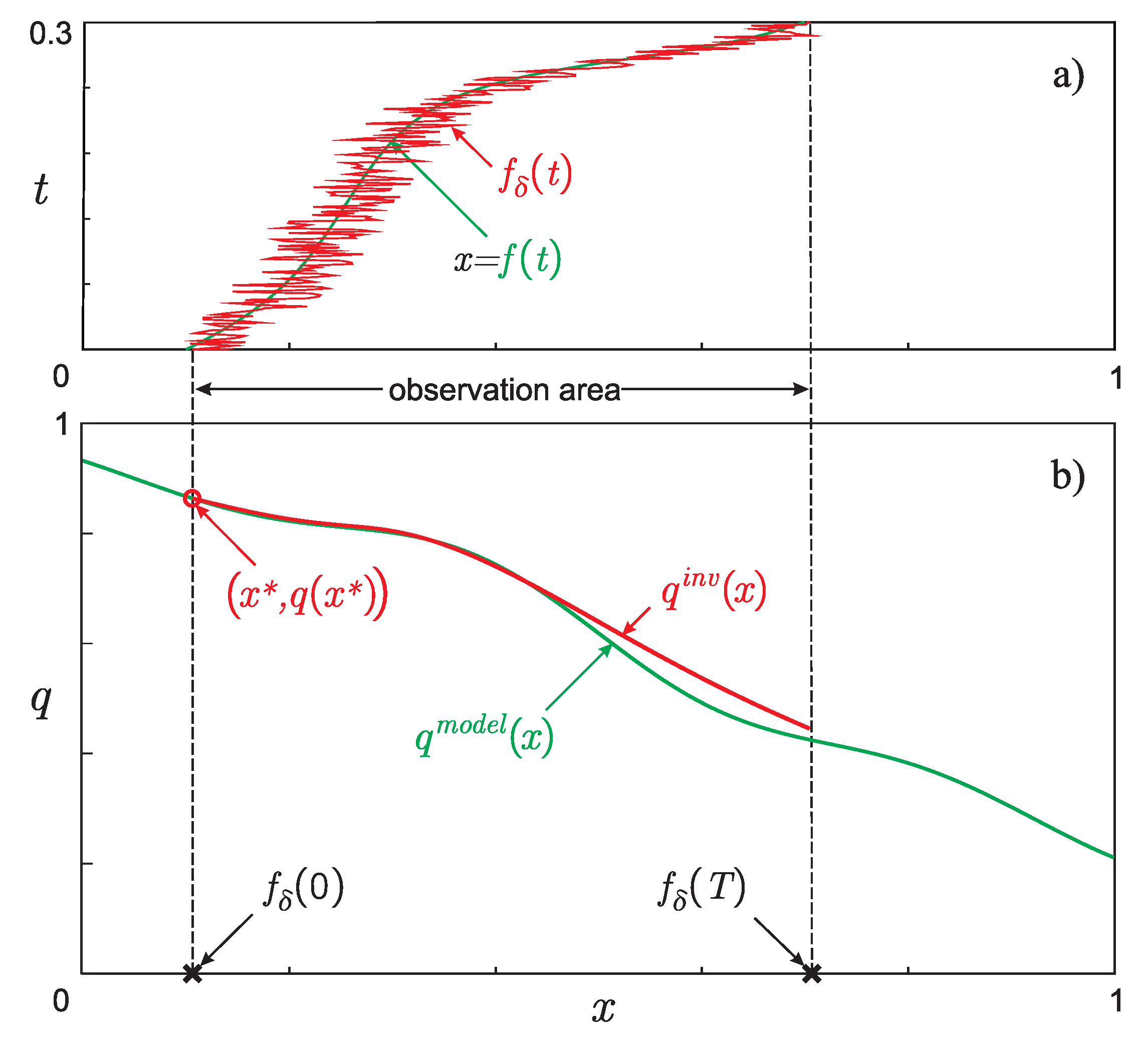
The boundary conditions $u_{left}$ and $u_{right}$ cannot be used as the initial condition for solving the reduced problem (19) and (20) even if it does not depend on t. This is due to the fact that unknown function $q\left(x\right)$ is defined by (19) only on the segment $x\in \left[f\left(0\right),f\left(T\right)\right]\subset [0,1]$ the autowave front passed through the experimental observation (see Figure 4). Thus, $x^{*}\in (0,1)$ (in other words, $x^{*}\ne 0$ or $x^{*}\ne 1$) when we observe the moving autowave front in the experiment.

(7)

There is no need to state and check the conditions for the existence of a front-type solution in the direct problem (1). We solved the inverse problem. Therefore, if we observe a moving autowave front, this means that the conditions for the existence of a solution of the front type are satisfied (whatever they may be).

(8)

The non-uniqueness of the solution to the inverse problem (1) and (2) is theoretically justified only if $\epsilon \to 0$. Having a fixed value of $\epsilon$ when solving a practical inverse problem, the non-uniqueness of the solution can only occur if the error $\delta$ of the input data $f_{\delta }\left(t\right)$ is sufficiently large. The question raised in Section 4.1 about the dependence $\delta \left(\epsilon \right)$, when the inverse problem (1) and (2) has a unique solution, remains open. This issue is of significant interest and may be the topic of separate work.

(9)

The recovered functions $\pm q\left(x\right)$ coincide with $u(x,t)$ at any fixed time moment $t\in [0,T]$ outside a small neighborhood of the autowave front localization point (see Figure 1). However, the values of the function $u(x,t)$ at a fixed-time instant can be much more difficult to observe experimentally than a clearly distinguishable contrast structure that determines the position of the interior layer (autowave front).

(10)

As was mentioned in the Introduction, the work was motivated by the example of flame propagation modeling in combustion theory [1] and the problem of modeling of habitat area movement in biophysics [2]. However, equations similar to the one considered in the work can occur in gas dynamics [48], chemical kinetics [49,50,51,52,53,54], nonlinear wave theory [3], biophysics [55,56,57,58], medicine [59,60,61,62], finance [63], and other fields of science [64].

6. Conclusions

We considered the features of the inverse problem formulation to recover the symmetric stable states of a bistable medium with data on the position of the autowave front propagating through it. Despite the ability demonstrated earlier in [20,21,28] for the successful solving of coefficient inverse problems for singularly perturbed equations with known data on the position of the reaction front, we managed to give an example of an applied problem in which additional information only on the front dynamics cannot be enough. It was shown that this formulation of the problem under certain conditions is ill-posed in the sense of the non-uniqueness of the solution. For a successful solution to the problem, additional information is required.

References

- Zeldovich, Y.; Barenblatt, G.; Librovich, V.; Makhviladze, G. The Mathematical Theory of Combustion and Explosions; Plenum: New York, NY, USA, 1985. [Google Scholar]
- Murray, J. Mathematical Biology. I. An Introduction; Springer: New York, NY, USA, 2002. [Google Scholar] [CrossRef]
- Volpert, A.; Volpert, V.; Volpert, V. Traveling Wave Solutions of Parabolic Systems; American Mathematical Society: Providence, RI, USA, 2000. [Google Scholar]
- Nefedov, N.; Nikulin, E. Existence and stability of periodic contrast structures in the reaction-advection-diffusion problem in the case of a balanced nonlinearity. Differ. Equ. 2017, 53, 516–529. [Google Scholar] [CrossRef]
- Davydova, M.; Nefedov, N. Multidimensional singularly perturbed reaction-diffusion-advection problems with a balanced nonlinearity and their applications in the theory of nonlinear heat conductivity. J. Physics Conf. Ser. 2019, 1205, 012011. [Google Scholar] [CrossRef]
- Sidorova, A.; Levashova, N.; Garaeva, A.; Tverdislov, V. A percolation model of natural selection. BioSystems 2020, 193, 104120. [Google Scholar] [CrossRef] [PubMed]
- Garaeva, A.; Sidorova, A.; Tverdislov, V.; Levashova, N. A model of speciation preconditions in terms of percolation and self-organized criticality theories. Biophysics 2020, 65, 795–809. [Google Scholar] [CrossRef]
- Cannon, J.; DuChateau, P. An Inverse problem for a nonlinear diffusion equation. SIAM J. Appl. Math. 1980, 39, 272–289. [Google Scholar] [CrossRef]
- DuChateau, P.; Rundell, W. Unicity in an inverse problem for an unknown reaction term in a reaction-diffusion equation. J. Differ. Equ. 1985, 59, 155–164. [Google Scholar] [CrossRef] [Green Version]
- Pilant, M.; Rundell, W. An inverse problem for a nonlinear parabolic equation. Commun. Partial. Differ. Equ. 1986, 11, 445–457. [Google Scholar] [CrossRef]
- Kabanikhin, S. Definitions and examples of inverse and ill-posed problems. J. Inverse Ill-Posed Probl. 2008, 16, 317–357. [Google Scholar] [CrossRef]
- Kabanikhin, S. Inverse and Ill-Posed Problems Theory and Applications; de Gruyter: Berlin, Germany, 2011. [Google Scholar]
- Jin, B.; Rundell, W. A tutorial on inverse problems for anomalous diffusion processes. Inverse Probl. 2015, 31, 035003. [Google Scholar] [CrossRef] [Green Version]
- Belonosov, A.; Shishlenin, M. Regularization methods of the continuation problem for the parabolic equation. Lect. Notes Comput. Sci. 2017, 10187, 220–226. [Google Scholar]
- Kaltenbacher, B.; Rundell, W. On the identification of a nonlinear term in a reaction-diffusion equation. Inverse Probl. 2019, 35, 115007. [Google Scholar] [CrossRef] [Green Version]
- Belonosov, A.; Shishlenin, M.; Klyuchinskiy, D. A comparative analysis of numerical methods of solving the continuation problem for 1D parabolic equation with the data given on the part of the boundary. Adv. Comput. Math. 2019, 45, 735–755. [Google Scholar] [CrossRef]
- Kaltenbacher, B.; Rundell, W. The inverse problem of reconstructing reaction-diffusion systems. Inverse Probl. 2020, 36, 065011. [Google Scholar] [CrossRef]
- Lukyanenko, D.; Shishlenin, M.; Volkov, V. Solving of the coefficient inverse problems for a nonlinear singularly perturbed reaction-diffusion-advection equation with the final time data. Commun. Nonlinear Sci. Numer. Simul. 2018, 54, 233–247. [Google Scholar] [CrossRef]
- Lukyanenko, D.; Prigorniy, I.; Shishlenin, M. Some features of solving an inverse backward problem for a generalized Burgers’ equation. J. Inverse Ill-Posed Probl. 2020, 28, 641–649. [Google Scholar] [CrossRef]
- Lukyanenko, D.; Borzunov, A.; Shishlenin, M. Solving coefficient inverse problems for nonlinear singularly perturbed equations of the reaction-diffusion-advection type with data on the position of a reaction front. Commun. Nonlinear Sci. Numer. Simul. 2021, 99, 105824. [Google Scholar] [CrossRef]
- Lukyanenko, D.; Grigorev, V.; Volkov, V.; Shishlenin, M. Solving of the coefficient inverse problem for a nonlinear singularly perturbed two-dimensional reaction-diffusion equation with the location of moving front data. Comput. Math. Appl. 2019, 77, 1245–1254. [Google Scholar] [CrossRef]
- Butuzov, V.; Vasilieva, A. Singularly perturbed problems with boundary and interior layers: Theory and applications. Adv. Chem. Phys. 1997, 97, 47–179. [Google Scholar]
- Vasilieva, A.; Butuzov, V.; Nefedov, N. Singularly perturbed problems with boundary and internal layers. Proc. Steklov Inst. Math. 2010, 268, 258–273. [Google Scholar] [CrossRef]
- Vasilieva, A.; Butuzov, V.; Kalachev, L. The Boundary Function Method for Singular Perturbation Problems; SIAM: Philadelphia, PA, USA, 1995. [Google Scholar]
- Fife, P.; McLeod, J. The approach of solutions of nonlinear diffusion. Equations to travelling front solutions. Arch. Ration. Mech. Anal. 1977, 65, 335–361. [Google Scholar] [CrossRef]
- Tikhonov, A.N.; Goncharsky, A.V.; Stepanov, V.V.; Yagola, A.G. Numerical Methods for the Solution of Ill-Posed Problems; Kluwer Academic Publishers: Dordrecht, The Netherlands, 1995. [Google Scholar]
- Lukyanenko, D.; Shishlenin, M.; Volkov, V. Asymptotic analysis of solving an inverse boundary value problem for a nonlinear singularly perturbed time-periodic reaction-diffusion-advection equation. J. Inverse Ill-Posed Probl. 2019, 27, 745–758. [Google Scholar] [CrossRef]
- Lukyanenko, D.; Yeleskina, T.; Prigorniy, I.; Isaev, T.; Borzunov, A.; Shishlenin, M. Inverse problem of recovering the initial condition for a nonlinear equation of the reaction-diffusion-advection type by data given on the position of a reaction front with a time delay. Mathematics 2021, 9, 342. [Google Scholar] [CrossRef]
- Klibanov, M.; Li, J.; Zhang, W. Convexification for an inverse parabolic problem. Inverse Probl. 2020, 36, 085008. [Google Scholar] [CrossRef]
- Klibanov, M.; Nguyen, D.L. Convergence of a series associated with the convexification method for coefficient inverse problems. J. Inverse -Ill-Posed Probl. 2020. [Google Scholar] [CrossRef]
- Leonov, A. Extra-Optimal Methods for Solving Ill-Posed Problems: Survey of Theory and Examples. Comput. Math. Math. Phys. 2020, 60, 960–986. [Google Scholar] [CrossRef]
- Bakushinskii, A.; Kokurin, M.; Kokurin, M. Direct and Converse Theorems for Iterative Methods of Solving Irregular Operator Equations and Finite Difference Methods for Solving Ill-Posed Cauchy Problems. Comput. Math. Math. Phys. 2020, 60, 915–937. [Google Scholar] [CrossRef]
- Kokurin, M. A posteriori choice of time-discretization step in finite difference methods for solving ill-posed Cauchy problems in Hilbert space. J. Inverse Ill-Posed Probl. 2021. [Google Scholar] [CrossRef]
- Lin, G.; Cheng, X.; Zhang, Y. A parametric level set based collage method for an inverse problem in elliptic partial differential equations. J. Comput. Appl. Math. 2018, 340, 101–121. [Google Scholar] [CrossRef] [Green Version]
- Gulliksson, M.; Holmbom, A.; Persson, J.; Zhang, Y. A separating oscillation method of recovering the G-limit in standard and non-standard homogenization problems. Inverse Probl. 2016, 32, 025005. [Google Scholar] [CrossRef]
- Egger, H.; Engl, H.; Klibanov, M. Global uniqueness and Holder stability for recovering a nonlinear source term in a parabolic equation. Inverse Probl. 2005, 21, 271–290. [Google Scholar] [CrossRef]
- Zhang, Y.; Gong, R. Second order asymptotical regularization methods for inverse problems in partial differential equations. J. Comput. Appl. Math. 2020, 375, 112798. [Google Scholar] [CrossRef] [Green Version]
- Gavalec, M.; Plavka, J.; Ponce, D. Strong, Strongly Universal and Weak Interval Eigenvectors in Max-Plus Algebra. Mathematics 2020, 8, 1348. [Google Scholar] [CrossRef]
- Angiulli, G.; Versaci, M.; Calcagno, S. Computation of the Cutoff Wavenumbers of Metallic Waveguides with Symmetries by Using a Nonlinear Eigenproblem Formulation: A Group Theoretical Approach. Mathematics 2020, 8, 489. [Google Scholar] [CrossRef] [Green Version]
- Yagola, A.; Leonov, A.; Titarenko, V. Data errors and an error estimation for ill-posed problems. Inverse Probl. Eng. 2002, 10, 117–129. [Google Scholar] [CrossRef]
- Titarenko, V.; Yagola, A. Error estimation for ill-posed problems on piecewise convex functions and sourcewise represented sets. J. Inverse -Ill-Posed Probl. 2008, 16, 625–638. [Google Scholar] [CrossRef]
- Leonov, A. Which of inverse problems can have a priori approximate solution accuracy estimates comparable in order with the data accuracy. Numer. Anal. Appl. 2014, 7, 284–292. [Google Scholar] [CrossRef]
- Leonov, A. A posteriori accuracy estimations of solutions to ill-posed inverse problems and extra-optimal regularizing algorithms for their solution. Numer. Anal. Appl. 2012, 5, 68–83. [Google Scholar] [CrossRef]
- Kokurin, M. Accuracy estimates of regularization methods and conditional well-posedness of nonlinear optimization problems. J. Inverse Ill-Posed Probl. 2018, 26, 789–797. [Google Scholar] [CrossRef]
- Kokurin, M. Ill-Posed Nonlinear Optimization Problems and Uniform Accuracy Estimates of Regularization Methods. Numer. Funct. Anal. Optim. 2020, 41, 1887–1900. [Google Scholar] [CrossRef]
- Cherniha, R. New Q-conditional symmetries and exact solutions of some reaction–diffusion–convection equations arising in mathematical biology. J. Math. Anal. Appl. 2007, 326, 783–799. [Google Scholar] [CrossRef] [Green Version]
- Cherniha, R.; Pliukhin, O. New conditional symmetries and exact solutions of nonlinear reaction-diffusion-convection equations. J. Phys. Math. Theor. 2007, 40, 10049–10070. [Google Scholar] [CrossRef] [Green Version]
- Danilov, V.; Maslov, V.; Volosov, K. Mathematical Modelling of Heat and Mass Transfer Processes; Kluwer: Dordrecht, The Netherlands, 1995. [Google Scholar]
- Liu, Z.; Liu, Q.; Lin, H.C.; Schwartz, C.; Lee, Y.H.; Wang, T. Three-dimensional variational assimilation of MODIS aerosol optical depth: Implementation and application to a dust storm over East Asia. J. Geophys. Res. Atmos. 2010, 116. [Google Scholar] [CrossRef] [Green Version]
- Egger, H.; Fellner, K.; Pietschmann, J.F.; Tang, B.Q. Analysis and numerical solution of coupled volume-surface reaction-diffusion systems with application to cell biology. Appl. Math. Comput. 2018, 336, 351–367. [Google Scholar] [CrossRef] [Green Version]
- Yaparova, N. Method for determining particle growth dynamics in a two-component alloy. Steel Transl. 2020, 50, 95–99. [Google Scholar] [CrossRef]
- Wu, X.; Ni, M. Existence and stability of periodic contrast structure in reaction-advection-diffusion equation with discontinuous reactive and convective terms. Commun. Nonlinear Sci. Numer. Simul. 2020, 91, 105457. [Google Scholar] [CrossRef]
- Lin, G.; Zhang, Y.; Cheng, X.; Gulliksson, M.; Forssén, P.; Fornstedt, T. A regularizing Kohn–Vogelius formulation for the model-free adsorption isotherm estimation problem in chromatography. Appl. Anal. 2018, 97, 13–40. [Google Scholar] [CrossRef]
- Zhang, Y.; Lin, G.; Gulliksson, M.; Forssén, P.; Fornstedt, T.; Cheng, X. An adjoint method in inverse problems of chromatography. Inverse Probl. Sci. Eng. 2017, 25, 1112–1137. [Google Scholar] [CrossRef]
- Meinhardt, H. Models of Biological Pattern Formation; Academic Press: London, UK, 1982. [Google Scholar]
- FitzHugh, R. Impulses and physiological states in theoretical model of nerve membrane. Biophys. J. 1961, 1, 445–466. [Google Scholar] [CrossRef] [Green Version]
- Egger, H.; Pietschmann, J.F.; Schlottbom, M. Identification of nonlinear heat conduction laws. J. Inverse Ill-Posed Probl. 2015, 23, 429–437. [Google Scholar] [CrossRef] [Green Version]
- Gholami, A.; Mang, A.; Biros, G. An inverse problem formulation for parameter estimation of a reaction-diffusion model of low grade gliomas. J. Math. Biol. 2016, 72, 409–433. [Google Scholar] [CrossRef] [Green Version]
- Aliev, R.; Panfilov, A. A simple two-variable model of cardiac excitation. Chaos Solitons Fractals 1996, 7, 293–301. [Google Scholar] [CrossRef]
- Generalov, E.; Levashova, N.; Sidorova, A.; Chumankov, P.; Yakovenko, L. An autowave model of the bifurcation behavior of transformed cells in response to polysaccharide. Biophysics 2017, 62, 876–881. [Google Scholar] [CrossRef]
- Mang, A.; Gholami, A.; Davatzikos, C.; Biros, G. PDE-constrained optimization in medical image analysis. Optim. Eng. 2018, 19, 765–812. [Google Scholar] [CrossRef] [Green Version]
- Kabanikhin, S.; Shishlenin, M. Recovering a Time-Dependent Diffusion Coefficient from Nonlocal Data. Numer. Anal. Appl. 2018, 11, 38–44. [Google Scholar] [CrossRef]
- Isakov, V.; Kabanikhin, S.; Shananin, A.; Shishlenin, M.; Zhang, S. Algorithm for determining the volatility function in the Black-Scholes model. Comput. Math. Math. Phys. 2019, 59, 1753–1758. [Google Scholar] [CrossRef]
- Kadalbajoo, M.; Gupta, V. A brief survey on numerical methods for solving singularly perturbed problems. Appl. Math. Comput. 2010, 217, 3641–3716. [Google Scholar] [CrossRef]
Publisher’s Note: MDPI stays neutral with regard to jurisdictional claims in published maps and institutional affiliations. |
© 2021 by the authors. Licensee MDPI, Basel, Switzerland. This article is an open access article distributed under the terms and conditions of the Creative Commons Attribution (CC BY) license (https://creativecommons.org/licenses/by/4.0/).
Share and Cite
Levashova, N.; Gorbachev, A.; Argun, R.; Lukyanenko, D. The Problem of the Non-Uniqueness of the Solution to the Inverse Problem of Recovering the Symmetric States of a Bistable Medium with Data on the Position of an Autowave Front. Symmetry 2021, 13, 860. https://doi.org/10.3390/sym13050860
Levashova N, Gorbachev A, Argun R, Lukyanenko D. The Problem of the Non-Uniqueness of the Solution to the Inverse Problem of Recovering the Symmetric States of a Bistable Medium with Data on the Position of an Autowave Front. Symmetry. 2021; 13(5):860. https://doi.org/10.3390/sym13050860
Chicago/Turabian StyleLevashova, Natalia, Alexandr Gorbachev, Raul Argun, and Dmitry Lukyanenko. 2021. "The Problem of the Non-Uniqueness of the Solution to the Inverse Problem of Recovering the Symmetric States of a Bistable Medium with Data on the Position of an Autowave Front" Symmetry 13, no. 5: 860. https://doi.org/10.3390/sym13050860