Novel Algorithms for Graph Clustering Applied to Human Activities

Abstract

In this paper, a novel algorithm (IBC1) for graph clustering with no prior assumption of the number of clusters is introduced. Furthermore, an additional algorithm (IBC2) for graph clustering when the number of clusters is given beforehand is presented. Additionally, a new measure of evaluation of clustering results is given—the accuracy of formed clusters (T). For the purpose of clustering human activities, the procedure of forming string sequences are presented. String symbols are gained by modeling spatiotemporal signals obtained from inertial measurement units. String sequences provided a starting point for forming the complete weighted graph. Using this graph, the proposed algorithms, as well as other well-known clustering algorithms, are tested. The best results are obtained using novel IBC2 algorithm: T = 96.43%, Rand Index (RI) 0.966, precision rate (P) 0.918, recall rate (R) 0.929 and balanced F-measure (F) 0.923.

1. Introduction

Automatic human activity recognition (HAR) development is a challenging task that is yet to be solved. The solution to this task has significant importance for improving human-machine interactions, security, healthcare and many other fields.

As computing hardware becomes more attainable, smaller and faster, it also becomes omnipresent, so much that presently, a smart phone, smart watch or similar accessory has assumed an integral role in everyday life. The upsurge of such wearable devices equipped with inertial measurement units (IMUs) brought an increase in the employment of IMU data for HAR. Implementation of various methods, using IMU for HAR, yields notable results in a field of automatic recognition on conventional HAR data sets, which contain solely simple and repetitive activities shown in [1,2,3,4,5]. However, the demand arises for analyzing complex activities which are not precisely defined. Various human subjects perform the same activity in different ways. Segments of the same complex activity can be performed in a different order. Additionally, different types of complex activities might have the same segments. Graph clustering algorithms [6,7,8,9] can be practical for human activities recognition and classification. The aim is to construct an algorithm suitable for human activities clustering, albeit there are significant inter-cluster similarities. A new graph-based clustering algorithm, suitable for analyzing both simple and complex human activities, is proposed in this paper. IMU data, less challenging for computational processing and considered suited for practical application, are used for testing the algorithm. Sequences of strings are configured, obtained from symbol-based modeling of spatiotemporal signals using IMU data. Sequences of strings can be understood as weighted graph vertices, whereby the weight of an edge presents a modified Levenshtein distance [10] between its vertices.

The first contribution of this paper is a novel clustering algorithm with no prior assumption of the number of clusters, which differs from noted hierarchical and non-hierarchical algorithms since it is based on a non-disjunct sets of vertices (not on a partition of all graph vertices). The algorithm is not built solely on connectivity or just on the distance of graph vertices but integrates both principles. The problem with all the algorithms is inter-cluster edges whose weights are less than the weights of some intra-cluster edges (the weight of the edges is inversely proportional to the similarity of the vertices); let us call them intruder edges. The algorithm recognizes and removes the intruder edges. Therefore, it is suitable for graph clustering with a significant percentage of intruder edges. Clusters obtained with the previous algorithm provide the starting point for an additional clustering algorithm with the number of clusters given beforehand. The additional algorithm (which represents the second contribution of this paper) delivers even more precise results. The third contribution is a new measure for the evaluation of clustering – the accuracy of formed clusters. This measure yields the percentage of common vertices of both given and corresponding formed clusters out of all the vertices. The fourth contribution imparts a theoretical basis for building sequences of strings, used for applying the described algorithms on clustering human activities and builds upon [10,11].

The introduced method is applied on two public data sets [12,13]. For comparison studies, four well-known algorithms are tested on the same samples. The novel algorithms give remarkable results over well-known algorithms. The proposed method can help filling the gap in increasing demand for research in complex HAR.

This paper consists of Section 1 Introduction, Section 7 Conclusion and five more sections. Section 2 consists of two subsections in which the two main contributions of this paper are presented. Section 2.1 presents a novel clustering algorithm with no prior assumption of the number of clusters. In Section 2.2 additional clustering algorithm when the number of clusters given beforehand is presented. In Section 3, a new measure for the evaluation of clustering results is presented—the Accuracy of formed clusters. In Section 4 string sequences formation and measure of similarity are displayed. Section 5 consists of three subsections. Section 5.1 shows the processing of data sets. In Section 5.2, results of testing are displayed and the parameters for the evaluation of clustering results are calculated. In Section 5.3, the comparative results of various algorithms and methods for clustering human activities are shown. Section 6 presents the discussion.

2. Graph Clustering

In this section, the clustering of a complete weighted graph is considered. First, a novel intruder-based clustering algorithm (IBC1) in the case with no prior assumption of the number of clusters is introduced. Second, in a case when the number of clusters is given beforehand, an additional algorithm (IBC2) is proposed.

Primarily, the terms used in this segment should be defined. Weighted graph edges, whose vertices are in the same cluster, are named intra-cluster edges and those whose vertices are in different clusters are named inter-cluster edges. The weight of some inter-cluster edge may be less than the weight of some intra-cluster edge. That type of inter-cluster edge is called an intruder edge. Now, the definition of an intruder of some vertex will be stated.

Let it be given a set $K=\{x_1,\dots ,x_n,\widehat{x}\}$, whose elements are vertices of a weighted graph where $K_0=\{x_1,\dots ,x_n\}$ is a cluster. With $d(a,b)$ the distance of graph vertices $a$ and $b$ is denoted, i.e., the weight of the edge $(a,b)$. Let

$$d=max\{d(x_i,x_j),x_i,x_j\in K_0\}.$$

(1)

Then $\widehat{x}$ is an intruder that corresponds to the vertex $x_k\in K_0$, if the following conditions are met:

$$d(x_k,\widehat{x})<d,\widehat{x}\ne x_i,i=1,2,\dots ,n.$$

(2)

Two factors can affect the appearance of an intruders. First, pairs of vertices in a cluster with a relatively large distance between them. Second, pairs of vertices from different clusters with a relatively small distances between them. The goal is to create an algorithm for graph clustering that is suitable for graphs with significant inter-cluster similarities. For the measure of the said similarity, the number of intruders can be used. Vertices of such graph have a significant number of intruders. Since the numbers of vertices in clusters is unknown, it is more appropriate to use the percentage than the number of intruders.

In this paper, graphs are observed, whose number of intruders corresponding to the vertex x of the cluster $K_x$, can be no more than $p\%$ of the total number of vertices of cluster $K_x$. Some intruders might be correspondent for more than one vertex of $K_x$. Furthermore, for every vertex, is left the $p\%$ possibility of removal of intra-cluster edges during the algorithm. The basic idea is recognition and removal of all inter-cluster edges. Naturally, the heaviest edges are examined first. During the iteration process, edge by edge is removed. The entire structure, all mutual adjacent vertices of the examined edge vertices, is analyzed. That structure, if in a cluster, should be strongly interconnected, with a limited number of additional edges (intruder edges) connected to it.

2.1. Graph Clustering with No Prior Assumption of the Number of Clusters

Let V be the set of all vertices of the weighted graph G. If vertices a and b ($a,b\in G$) are connected with an edge, then that edge is denoted with an unordered pair $(a,b)$. Let

$$k=((a_1,b_1),(a_2,b_2),\dots ,(a_m,b_m))$$

(3)

be a sequence of graph edges so that weights of edges form a non-descending sequence (further in the text, a non-descending sequence of edges). Furthermore, the mapping is defined

$${\mathcal{F}}_k:V⟶P\left(V\right),$$

(4)

where $P\left(V\right)$ is a power set of a set V, in a following way:

$${\mathcal{F}}_k\left(x\right)=\left\{x\right\}\cup \{x_i\in V|(x,x_i)\mathrm{is} \mathrm{from} \mathrm{the} \mathrm{sequence} k \left(3\right)\}.$$

(5)

In continuation ${\mathcal{F}}_k\left(x\right)$ is denoted as X. Thus, to every vertex x a set X is assigned, whose elements are that vertex and all its adjacent vertices from the edge sequence k (3).

Furthermore, description of IBC1 algorithm is given.

Step one: The weight-based non-descending sequence of edges is established. Then, the average distance between all graph vertices (arithmetic mean of edge weights) is calculated. It is considered that pair of vertices, whose distance is greater than average are not similar, i.e., they do not belong to the same cluster. Vertices, whose distances from other vertices is greater than average, are single-member clusters. Let c be a non-descending sequence of edges whose weight is less than average.

Step two: The heaviest edge is selected, specifically the best candidate for an inter-cluster edge from the edge sequence

$$c=((a_1,b_1),(a_2,b_2),\dots ,(a_M,b_M)).$$

(6)

Three cases are distinguished:

(A)

The weight of the last edge $(a_M,b_M)$ in the sequence differs from the weights of the other edges of a sequence and that edge is marked with $(x,y)$.

(B)

The last r edges in a sequence

$$(a_{M-(r-1)},b_{M-(r-1)}),\dots ,(a_M,b_M)$$

(7)

have the same weight and

$$card(A_i\cap B_i),(i=M-(r-1),\dots ,M)$$

(8)

has the unique smallest value, where $A_i={\mathcal{F}}_c\left(a_i\right)$ and $B_i={\mathcal{F}}_c\left(b_i\right)$. Let that smallest value correspond to the edge that is marked with $(x,y).$

(C)

The last r edges (7) in a sequence have the same weight and a few (8) have the same smallest value. From the edges that have the same smallest value, one edge is selected that is marked with $(x,y).$

Let the $(x,y)$ edge be determined in any of the previous three cases. No two cases can occur simultaneously

Let

$${\mathcal{F}}_c\left(x\right)=X=\{x,y,x_1,\dots ,x_n,{\widehat{x}}_1,{\widehat{x}}_2,\dots ,{\widehat{x}}_k\}$$

(9)

$${\mathcal{F}}_c\left(y\right)=Y=\{x,y,x_1,\dots ,x_n,{\widehat{y}}_1,{\widehat{y}}_2,\dots ,{\widehat{y}}_s\}$$

(10)

Some of the sets $\{x_1,\dots ,x_n\}$, $\{{\widehat{x}}_1,{\widehat{x}}_2,\dots ,{\widehat{x}}_k\}$, $\{{\widehat{y}}_1,{\widehat{y}}_2,\dots ,{\widehat{y}}_s\}$ can be empty sets.

Step three: A set of cluster candidates is formed

$$Z=X\cap Y=\{x,y,x_1,\dots ,x_n\}.$$

(11)

Set Z is not empty since it contains vertices x and y at least. Vertices from sets X and Y, that do not belong to Z, are candidates for intruders. Furthermore, two alternatives are distinguished:

(i) If

$$k>(n+2)\frac{p}{100}\mathrm{or}s>(n+2)\frac{p}{100}.$$

(12)

Then, it is considered that vertices x and y do not belong to the same cluster. Edge $(x,y)$ is removed from the sequence. After the removal, a new sequence that has one edge less is gained and it will be marked with c, again. Then the return to the second step follows.

(ii) If

$$k⩽(n+2)\frac{p}{100}\mathrm{and}s⩽(n+2)\frac{p}{100}.$$

(13)

Then, it is examined if any of the edges $(x,{\widehat{y}}_j),j=1,\dots ,s$, $(y,{\widehat{x}}_i),i=1,\dots ,k$ is intra-cluster, that is removed throughout algorithm execution. For each remaining element ${\widehat{x}}_i$ from X and ${\widehat{y}}_j$ from Y, if any, it is checked if it is contained in $(100-p)\%$ sets assigned to elements of the set Z. All the vertices that do not satisfy the previous condition are intruders. To every vertex ${\widehat{x}}_i$, that is ${\widehat{y}}_j$, the set ${\widehat{X}}_i={\mathcal{F}}_c\left({\widehat{x}}_i\right)$ is assigned, that is ${\widehat{Y}}_j={\mathcal{F}}_c\left({\widehat{y}}_j\right)$. Then the set is determined

$$\begin{array}{ccc}\hfill \widehat{Z}& =& \left\{{\widehat{x}}_i|card(Z\backslash {\widehat{X}}_i)⩽card\left(Z\right)\frac{p}{100}\right\}\hfill \\ & \bigcup & \left\{{\widehat{y}}_j|card(Z\backslash {\widehat{Y}}_j)⩽card\left(Z\right)\frac{p}{100}\right\}.\hfill \end{array}$$

(14)

New set of candidates for a cluster is

$$Z^{+}=Z\cup \widehat{Z},$$

(15)

where $\widehat{Z}$ can be an empty set. Then, for every $x_i\in Z^{+}$ it is checked to what extent it is connected to other vertices from $Z^{+}$. That is why the sets are determined

$$X^i=X_i\cap Z^{+},$$

(16)

where $X_i$ is a set assigned to vertex $x_i\in Z^{+}$. The overlaps of the sets $Z^{+}$ and $X^i$ are checked. Set $Z^{+}$ may contain intruders common to x and y. Additionally, there may have been a previous removal of intra-cluster edges that contain vertex $x_i$. Additionally, it is checked whether the number of intruders corresponding to the vertex $x_i$ is within the presumed limits. It is examined in the following way. If

$$card(Z^{+}\backslash X^i)>card\left(Z^{+}\right)\frac{p}{100}\vee card(X_i\backslash X^i)>card\left(X_i\right)\frac{p}{100},$$

(17)

it is considered that vertex $x_i$ does not belong to the cluster of the vertex x. Then it is determined

$$\begin{array}{ccc}\hfill K_X& =& \left\{x_i\in Z^{+}|card(Z^{+}\backslash X^i)⩽card\left(Z^{+}\right)\frac{p}{100}\right\}\hfill \\ & \bigcap & \left\{x_i\in Z^{+}|card(X_i\backslash X^i)⩽card\left(X_i\right)\frac{p}{100}\right\}.\hfill \end{array}$$

(18)

Except the common intruders for x and y, all the other elements from $Z^{+}$ are in $K_X$. It is resumed examining whether it is

$$card\left(Z^{+}\right)-card\left(K_x\right)>card\left(K_x\right)\frac{p}{100}.$$

(19)

If the inequality (19) holds, it is considered that $K_x$ is not a cluster and that edge $(x,y)$ is inter-cluster. The edge $(x,y)$ is removed from the sequence. After the removal, a new sequence that has one edge less is obtained and it will be marked with c again. Then return to the second step follows.

If the inequality (19) does not hold, it is considered $K_x$ to be a cluster containing the vertex x. All the edges containing some of the vertices of a formed cluster are removed from the sequence. After the removal, a new sequence with fewer edges is gained which will be marked with c again. If all clusters are not formed (i.e., not all edges are removed from sequence), the return to the second step follows.

The first and second steps of this algorithm are based exclusively on the distance between the two vertices. The third step is based solely on the connectivity of the vertices.

2.2. Graph Clustering When the Number of Clusters Is Given Beforehand

Furthermore, description of IBC2 algorithm is given.

In the algorithm described in the preceding segment, it is assumed that the number of clusters is unknown. Provided that the number of clusters is known, let it be said n, the previous algorithm determines the clusters that serve as the starting point (base clusters) for more precise determination of final clusters. It is assumed that the clusters have approximately the same number of vertices. If the number of base clusters is less than n, the described algorithm cannot determine the required clusters.

First step: If the number of base clusters is equal to n, all base clusters are final clusters as well. Furthermore, only the case when the number of base clusters is greater than n is considered.

Let

$$(K_1,K_2,\dots ,K_m)$$

(20)

be a sequence of all base clusters where

$$(card\left(K_1\right),card\left(K_2\right),\dots ,card\left(K_m\right))$$

(21)

is a non-ascending sequence. Two cases are distinguished:

1. There is j where

$$j=\underset{\genfrac{}{}{0pt}{}{n⩽i<m}{card\left(K_i\right)\ne card\left(K_{i+1}\right)}}{min}i$$

(22)

In this case, candidates for new base clusters are following

$$K_1,K_2,\dots ,K_j.$$

(23)

2. If such j does not exist, then the last $k(k>m-n)$ base clusters in the sequence (20) have the same number of vertices. For each of the last k base clusters from the sequence, the average distance between all its vertices is determined. Candidates for new base clusters remain all the base clusters except for the one with largest average distance.

Second step: Furthermore, for each vertex of the base clusters, which are not a candidate after the first step, the average distance from all vertices of each candidate separately is determined. If the observed vertex has a minimum average distance from one or more candidates, that vertex is added to one of those candidates at the end of the check. After this step, all the candidates become the new base clusters. Then return to the first step follows.

This additional algorithm is based exclusively on distance between two vertices.

3. Evaluation Measures

First, a novel external evaluation measure, the Accuracy of formed clusters, is introduced.

Let all the clusters $C_1,C_2,\dots ,C_n$ of a complete weighted graph be given and let $\{K_1,K_2,\dots ,K_n\}$ be a collection of sets defined in the following way:

1. Using the process of clustering, if a derived cluster is obtained, which contains more than $50\%$ vertices of the cluster $C_i$ and no more than $50\%$ vertices of some other cluster $C_j$, than the cluster $K_i$ is equal to that derived cluster.

2. Using the process of clustering, if a derived cluster is obtained, which contains more than $50\%$ vertices of the cluster $C_i$ and more than $50\%$ vertices of some other cluster $C_j$ and $i⩽j$ than $K_i$ is equal to that derived cluster and $K_j=\varnothing$.

Furthermore, only derived clusters, that do not fulfil the conditions previously mentioned in cases 1. and 2., are considered.

3. If existing, a derived cluster, containing $50\%$ vertices of the cluster $C_i$ with the lowest index i, is determined first. Then $K_i$ is equal to the derived cluster. The process continues with the remaining given and derived clusters.

4. $K_i$ sets, which are not obtained using the previous process, are empty.

If $K_i$ is not an empty set, then $K_i$ is formed cluster that corresponding to $C_i$. The accuracy of formed clusters (T) is determined in the following way:

$$T=\frac{{\displaystyle \sum _{i=1}^n}card(C_i\cap K_i)}{{\displaystyle \sum _{i=1}^n}card\left(C_i\right)}·100\%$$

(24)

For evaluation of clustering results, besides the presented measure, the following evaluation measures are used.

The Rand Index ($RI$) computes how similar the derived clusters (returned by the clustering algorithm) are to the ground truth clusters. It can be computed using the following formula

$$RI=\frac{TP+TN}{TP+FP+FN+TN}$$

(25)

where $TP$ (number of true positives) is the number of pairs of points that are clustered together in the derived and ground truth partition, $TN$ (number of true negatives) is the number of pairs of points that are in different clusters in the derived and ground truth partition, $FP$ (number of false positives) is the number of pairs of points that are clustered together in the derived but not in the ground truth partition, and $FN$ (number of false negatives) is the number of pairs of points that are clustered together in the ground truth but not in the derived partition.

$$\mathrm{Precision}P=\frac{TP}{TP+FP}$$

(26)

$$\mathrm{Recall}R=\frac{TP}{TP+FN}$$

(27)

$$\mathrm{Balanced} \mathrm{F}-\mathrm{measure}F=\frac{2PR}{P+R}$$

(28)

The presented evaluation measure T (24) gives the percentage of common vertices of both given and corresponding formed clusters out of all the vertices. It has a certain similarity with Purity, which is a measure of the extent to which clusters contain a single class. Purity can be calculated as follows: for every observed cluster, it counts the number of data points of the most common class in that cluster. Then, sums over all clusters and divides by the total number of data points. Drawback of this measure is that in the case of great number of derived clusters, it can give high purity. For example, a purity score is 1 if each data point is in a single-member derived cluster. The measure T removes the said drawback.

Measures (25)–(28) are based on pairs of data points and therefore are not directly comparable with the proposed measure T. If pairs of data points from the same class belong to different derived clusters, then those pairs are considered true positive. By analogy with the proposed principle, true positive pairs of data points are only those true positive pairs belonging to formed clusters.

4. String Sequences Formation, Measure of Similarity of Two String Sequences

As a theoretical base for forming the sequences of strings, the following consideration can be used.

Let $I_k=\{1,2,\dots ,k\},J_n=\{1,2,\dots ,n\}$, represent sets where $k,n\in N$ and $k,n⩾2.$ Mapping is defined on a set $I_k\times J_n:$

$$p:I_k\times J_n⟶R,$$

(29)

where $p(i,j)=p_{ij}\in R.$ Using the mapping p is a determined matrix

$$P=\left(\begin{array}{cccc}{p}_{11}& p_{12}& \cdots & p_{1n}\\ p_{21}& p_{22}& \cdots & p_{2n}\\ \cdots & \cdots & \cdots & \cdots \\ p_{k1}& p_{k2}& \cdots & p_{kn}\end{array}\right)$$

(30)

Relations M and m are defined on a set $I_k\times J_n$ in the following way:

$$iMj⟺\left\{\begin{array}{ccc}{p}_{ij}>p_{(i+1)j}\hfill & \mathrm{if}\hfill & i=1\hfill \\ p_{ij}>p_{(i-1)j}\hfill & \mathrm{if}\hfill & i=n\hfill \\ p_{(i-1)j}<p_{ij}\wedge p_{ij}>p_{(i+1)j}\hfill & \mathrm{if}\hfill & 1<i<n,\hfill \end{array}\right.$$

(31)

$$imj⟺\left\{\begin{array}{ccc}{p}_{ij}<p_{(i+1)j}\hfill & \mathrm{if}\hfill & i=1\hfill \\ p_{ij}<p_{(i-1)j}\hfill & \mathrm{if}\hfill & i=n\hfill \\ p_{(i-1)j}>p_{ij}\wedge p_{ij}<p_{(i+1)j}\hfill & \mathrm{if}\hfill & 1<i<n.\hfill \end{array}\right.$$

(32)

It is clear that the following holds

$$(\forall i,j)\neg (iMj\wedge imj).$$

(33)

Using introduced relations, the mapping is defined

$$f:I_k\times J_n⟶S,$$

(34)

where

$$S=\{M_1,m_1,M_2,m_2,\dots ,M_n,m_n,\epsilon \}$$

(35)

is a set of symbols, in a following way:

$$f(i,j)=\left\{\begin{array}{ccc}{M}_j\hfill & \mathrm{if}\hfill & \tau \left(iMj\right)=\top \hfill \\ m_j\hfill & \mathrm{if}\hfill & \tau \left(imj\right)=\top \hfill \\ \epsilon \hfill & \hfill & \mathrm{otherwise}.\hfill \end{array}\right.$$

(36)

By mapping f the matrix is determined:

$$F=\left(\begin{array}{cccc}f(1,1)& f(1,2)& \cdots & f(1,n)\\ f(2,1)& f(2,2)& \cdots & f(2,n)\\ \cdots & \cdots & \cdots & \cdots \\ f(k,1)& f(k,2)& \cdots & f(k,n)\end{array}\right).$$

(37)

And let the mapping be defined

$$\phi :F⟶{(S_1,S_2,\dots ,S_k)}^T$$

(38)

so that

$$S_i=f(i,1)\oplus f(i,2)\oplus \cdots \oplus f(i,n),$$

(39)

where ⊕ stands for concatenation. In that way a sequence of strings is gained, whose symbols belong to the set S. Finally, the symbol $\epsilon$ is omitted in each string, as well as all the strings that contained only symbol $\epsilon$. This way, a sequence of strings is gained

$$a={({\widehat{S}}_1,{\widehat{S}}_2,\dots ,{\widehat{S}}_{\widehat{k}})}^T$$

(40)

where $\widehat{k}⩽k.$

Different parameters (e.g., angular velocity, instantaneous acceleration, absolute orientation), the values of which are obtained via measurement units, are used for the analysis of human activities.

Data from measurement units, arranged in temporal order, are shown in matrix P (30). The element $p_{ij},$$i=1,2,\dots ,k;$$j=1,2,\dots ,n$, of the matrix P, is the value of the parameter with the ordinal number j at the time point i. These n parameters have their local extrema (maxima and minima). The procedure for assigning symbols to these extrema is described. At the observed point in time, several parameters can have extreme values. From all the symbols assigned to the extrema, a string is formed at the observed time point. Strings arranged in temporal order form a sequence of strings.

The widely acknowledged Levenshtein distance ($\lambda$) [14] can be used as the measure of similarity between two strings. Informally, it is defined as the minimum number of single-character editing operations (deletion, insertion and substitution) needed to transform one string into the other. By the described symbol-based modeling of signals from measurement units, strings were obtained instead of characters, and a sequence of strings instead of string. Therefore, the adaptation of editing operations of Levenshtein distance is needed.

The adapted Levenshtein distance [10] used in this approach quantifies the similarity between two sequences of strings (40).

5. Evaluation

To apply the described algorithm to human activities clustering, symbols gained by modeling of spatiotemporal signals are needed, which are then used to form sequences of strings. Sequences of strings can be understood as weighted graph vertices, whereby the weight of an edge presents a modified Levenshtein distance between its vertices.

5.1. Databases, Preprocessing

To evaluate the proposed approach in a realistic environment, Carnegie Mellon University Multimodal Activity (CMU-MMAC) database [12] and RealWorld data set [13] are used. The first database presents complex, while the second presents simple human activities.

CMU-MMAC database contains recordings of human subjects preparing various recipes in the kitchen. One of the modalities found in this database is noted by the three-axis IMU (MicroStrain’s 3DM-GX1), containing an accelerometer, gyroscope and magnetometer, which enable the measurement of absolute orientation, angular velocity and instantaneous acceleration. The signals were gyro-stabilized and recorded at a frequency of 125 Hz. Twelve human subjects ($S40,S41,S42,S43,S44,S4,S50,S51,S52,S53,S54,S55$) are chosen, each of whom was recorded while preparing four different recipes (brownies, scrambled eggs, pizza and sandwich) i.e., performing four different activities. One of these 48 subject–activity pairs, subject $S52$ making brownies (S52, brownies) contained errors and was therefore excluded. All selected subjects are right-handed, so it is decided to observe signals collected from IMU placed on their right hand. At the signal level, angular velocity and instantaneous acceleration along three axes (six parameters in total) are specifically considered. As an illustration, the values of the parameters sampled in five consecutive time points that represent a minuscule fragment of the subject–activity pair (S51, Eggs), are given in

Table 1. Illustration of the input inertial measurement data.

Acceleration			Angular Velocity			Count	System Time
${\mathit{a}}_{\mathit{x}}$	${\mathit{a}}_{\mathit{y}}$	${\mathit{a}}_{\mathit{z}}$	Roll	Pitch	Yaw
0.003632	−0.500534	−0.183935	−0.005648	−0.555695	−0.629118	27,683	10:04:02:440
0.041871	−0.545610	−0.146977	0.278318	−0.599623	−0.668340	27,684	10:04:02:448
0.064516	−0.616962	−0.1523187	0.566050	−0.675871	−0.678695	27,685	10:04:02:456
0.085452	−0.758171	−0.182867	0.872607	−0.746784	−0.638845	27,686	10:04:02:464
0.096561	−0.878231	−0.172826	1.147788	−0.850643	−0.479762	27,687	10:04:02:472

. Aiming for efficiency, the data are down-sampled to a frequency of 1.25 Hz.

RealWorld data set contains recordings of 15 human subjects (age 31.9 ± 12.4, height 173.1 ± 6.9, weight 74.1 ± 13.8, eight males and seven females) performing fundamental activities of which four are considered: walking, climbing up the stairs, jumping and running. Two modalities found in this database—the three-axis accelerometer and gyroscope—are used. The signals are recorded at a frequency of 50 Hz. Due to the nature of analyzed activities, it is decided to observe signals collected from wearable device placed on the shin. At the signal level, angular velocity and instantaneous acceleration along three axes (six parameters in total) are considered. For efficiency, the sample is selected so that all activities last for 90 s. Additionally, selected data are down-sampled to a frequency of 2.5 Hz.

5.2. Results

Subject–activity pairs can be interpreted as vertices of a weighted graph. Each subject–activity pair has one corresponding sequence of strings. The set of vertices corresponding to the same activity forms a cluster (class). To perform clustering, it is needed to input the parameter p, which represents the maximum percentage of intruders, which is not known.

First, the results obtained from CMU-MMAC database are presented. The recipes for the dishes prepared by human subjects are not precisely defined, so different individuals prepare the same recipes in different manners. Additionally, there are a series of actions that are very similar in preparing different recipes. Based on the preceding, it is reasonable to assume that the percentage of intruders is not small. So that the parameter p can be determined more precisely, that is the upper bound of the percentage of intruders, the set of subjects is divided into two disjunct subsets. The first subset is $\{S40,S41,S42,S43,S44,S45\}$, and the second is $\{S50,S51,S52,S53,S54,S55\}$. The first subset, containing 24 subject–activity pairs, is used for training. The second subset is used for testing; it contains 23 subject–activity pairs. During the training, the criterion Accuracy of formed clusters was used to estimate the parameter p. According to this criterion, a result was obtained that was within the expected range, i.e., $p=30$. Operating with the same sample, two tests are performed. The first test was performed using the IBC1 algorithm Section 2.1, with no prior assumption of the number of clusters. Then, the testing was performed on the same sample using the IBC2 algorithm Section 2.2, when the number of clusters is given beforehand, i.e., in the observed sample is four. The results of clustering are shown in

Table 2. Clustering results, with no prior assumption of the number of clusters, obtained by IBC1 algorithm using CMU-MMAC database.

Subject, Activity	Clusters
	C1	C2	C3	C4	C5	C6
S50, Brownie	x
S51, Brownie	x
S53, Brownie					x
S54, Brownie	x
S55, Brownie	x
S50, Eggs		x
S51, Eggs		x
S52, Eggs		x
S53, Eggs		x
S54, Eggs		x
S55, Eggs		x
S50, Pizza			x
S51, Pizza			x
S52, Pizza					x
S53, Pizza			x
S54, Pizza			x
S55, Pizza			x
S50, Sandwich						x
S51, Sandwich				x
S52, Sandwich				x
S53, Sandwich				x
S54, Sandwich				x
S55, Sandwich				x

and

Table 3. Clustering results, when the number of clusters is given beforehand, obtained by IBC2 algorithm using CMU-MMAC database.

Subject, Activity	Clusters
	C1	C2	C3	C4
S50, Brownie	x
S51, Brownie	x
S53, Brownie	x
S54, Brownie	x
S55, Brownie	x
S50, Eggs		x
S51, Eggs		x
S52, Eggs		x
S53, Eggs		x
S54, Eggs		x
S55, Eggs		x
S50, Pizza			x
S51, Pizza			x
S52, Pizza	x
S53, Pizza			x
S54, Pizza			x
S55, Pizza			x
S50, Sandwich				x
S51, Sandwich				x
S52, Sandwich				x
S53, Sandwich				x
S54, Sandwich				x
S55, Sandwich				x

, in cases with no prior assumption on the number of clusters and when the number of clusters is given beforehand, respectively. To make the evaluation more complete, the Rand Index, precision, recall and balanced F-measure are calculated. Values of evaluation parameters are displayed as follows:

Table 4. Evaluation of clustering results obtained by IBC1 algorithm using CMU-MMAC database.

Accuracy of Formed Clusters		$\mathit{T}=86.96\%$
True positives	$TP=41$	Rand index	$RI=0.941$
True negatives	$TN=197$	Precision	$P=0.976$
False positives	$FP=1$	Recall	$R=0.745$
False negatives	$FN=14$	Balanced F-measure	$F=0.845$

in a case with no prior assumption on the number of clusters;

Table 5. Evaluation of clustering results obtained by IBC2 algorithm using CMU-MMAC database.

Accuracy of Formed Clusters		$\mathit{T}=95.65\%$
True positives	$TP=50$	Rand index	$RI=0.960$
True negatives	$TN=193$	Precision	$P=0.909$
False positives	$FP=5$	Recall	$R=0.909$
False negatives	$FN=5$	Balanced F-measure	$F=0.909$

in a case when the number of clusters is given beforehand.

Furthermore, the results obtained from RealWorld data set are presented. The set of subjects, each of whom was recorded while performing four different activities (walking, climbing up the stairs, jumping and running) is divided into two disjunct subsets. The first subset is $\{S1,S2,S3,S4,S5,S6,S7,S8\}$, and the second is $\{S9,S10,S11,S12,S13,S14,S15\}$. The first subset, containing 31 subject–activity pairs (data for subject $S3$ is missing for one activity), is used for training. The second subset, is used for testing; it contains 28 subject–activity pairs. By applying the criterion, Accuracy of formed clusters, the parameter $p=15$ is obtained. Operating with the same sample, two tests are performed. First, using the IBC1 algorithm with no prior assumption of the number of clusters, then, using the IBC2 algorithm where it is assumed that the number of clusters is four.

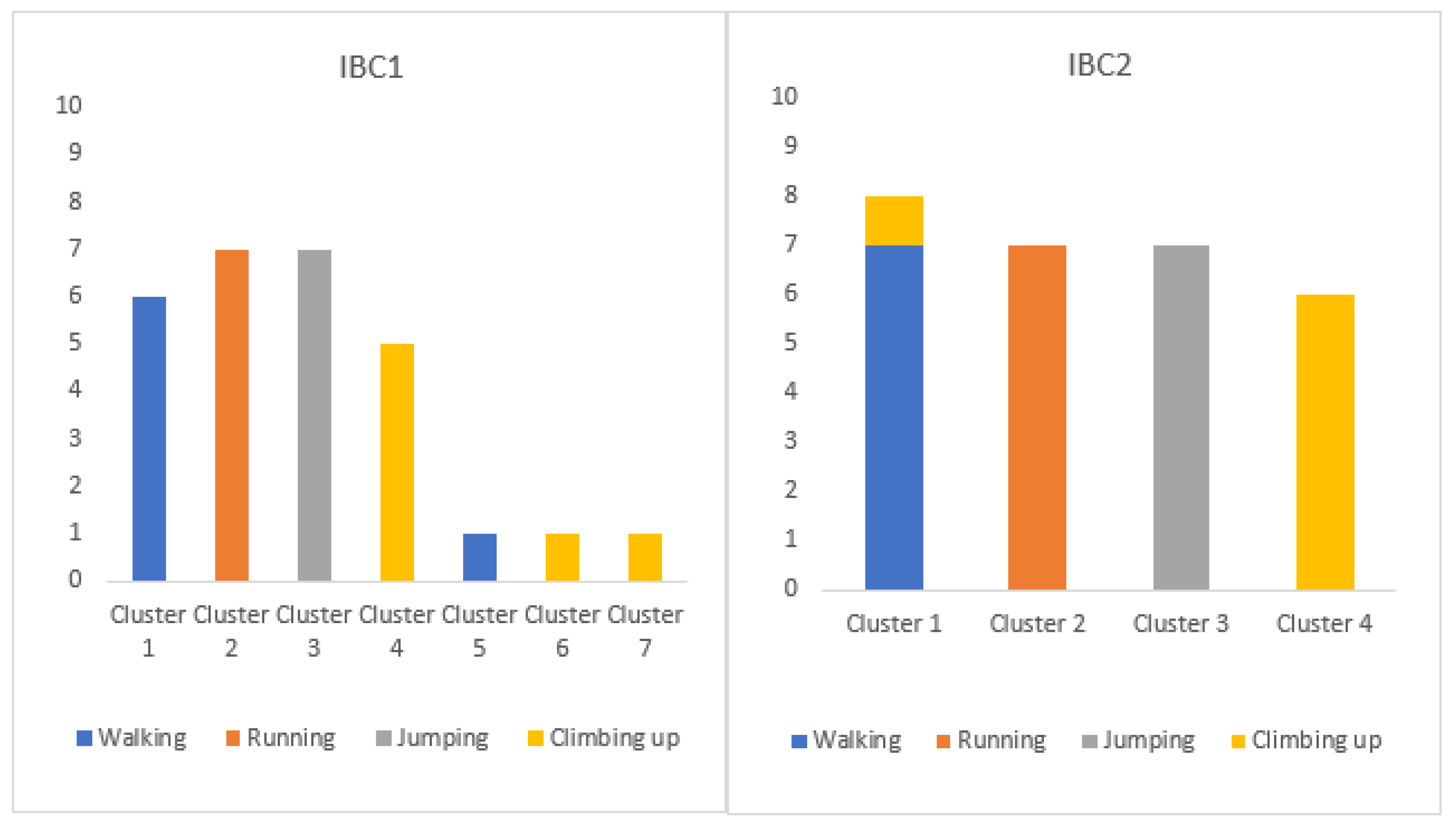
The results of clustering are given in Figure 1.

For more comprehensible evaluation, the Rand Index, precision, recall and balanced F-measure are presented in

Table 6. Evaluation of clustering results obtained by IBC1 algorithm using RealWorld data set.

Accuracy of Formed Clusters		$\mathit{T}=89.29\%$
True positives	$TP=67$	Rand index	$RI=0.955$
True negatives	$TN=294$	Precision	$P=1$
False positives	$FP=0$	Recall	$R=0.798$
False negatives	$FN=17$	Balanced F-measure	$F=0.888$

and

Table 7. Evaluation of clustering results obtained by IBC2 algorithm using RealWorld data set.

Accuracy of Formed Clusters		$\mathit{T}=96.43\%$
True positives	$TP=78$	Rand index	$RI=0.966$
True negatives	$TN=287$	Precision	$P=0.918$
False positives	$FP=7$	Recall	$R=0.929$
False negatives	$FN=6$	Balanced F-measure	$F=0.923$

; in a case with no prior assumption of the number of clusters and when the number of clusters is given beforehand, respectively.

5.3. Comparative Results

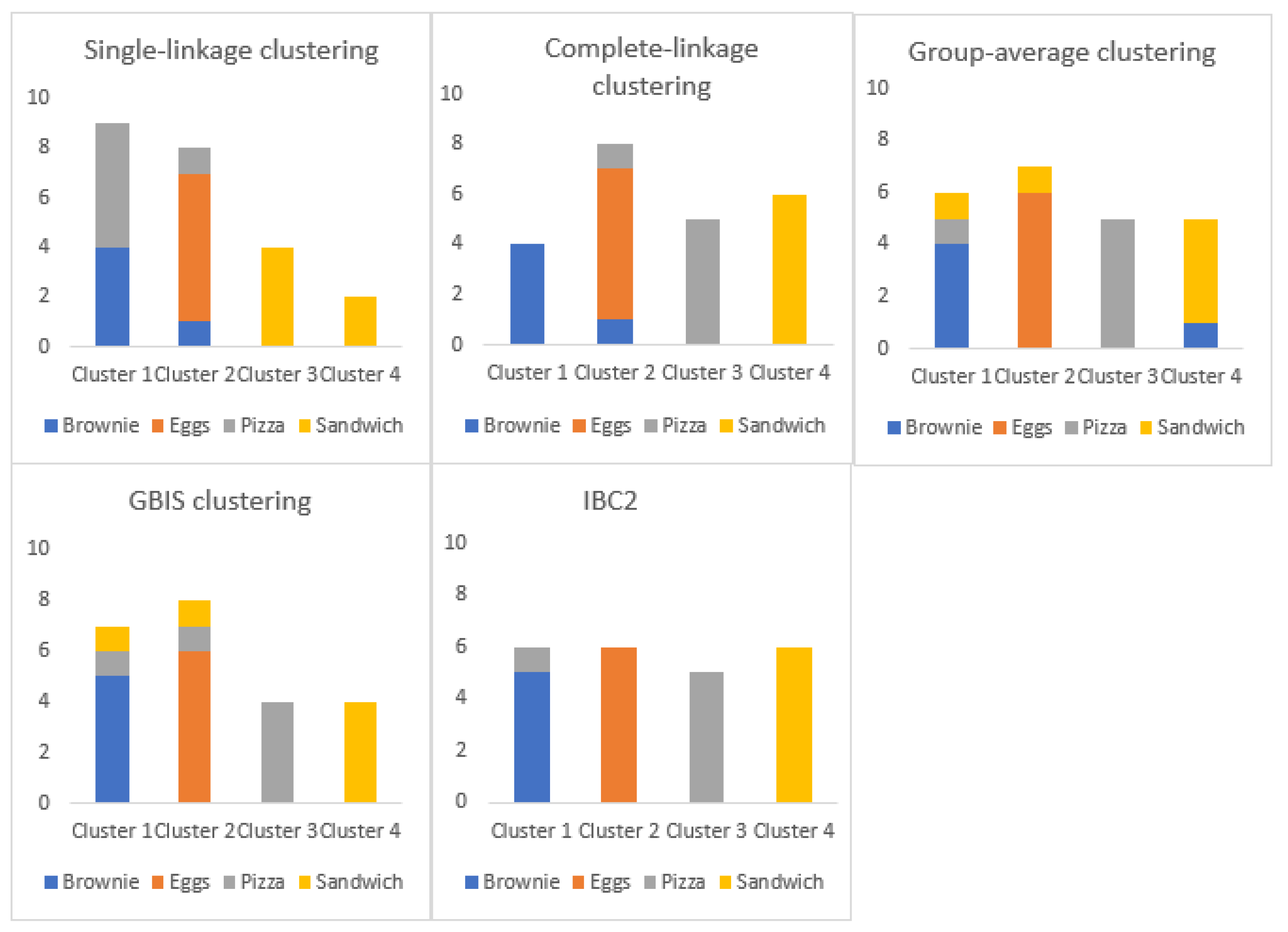
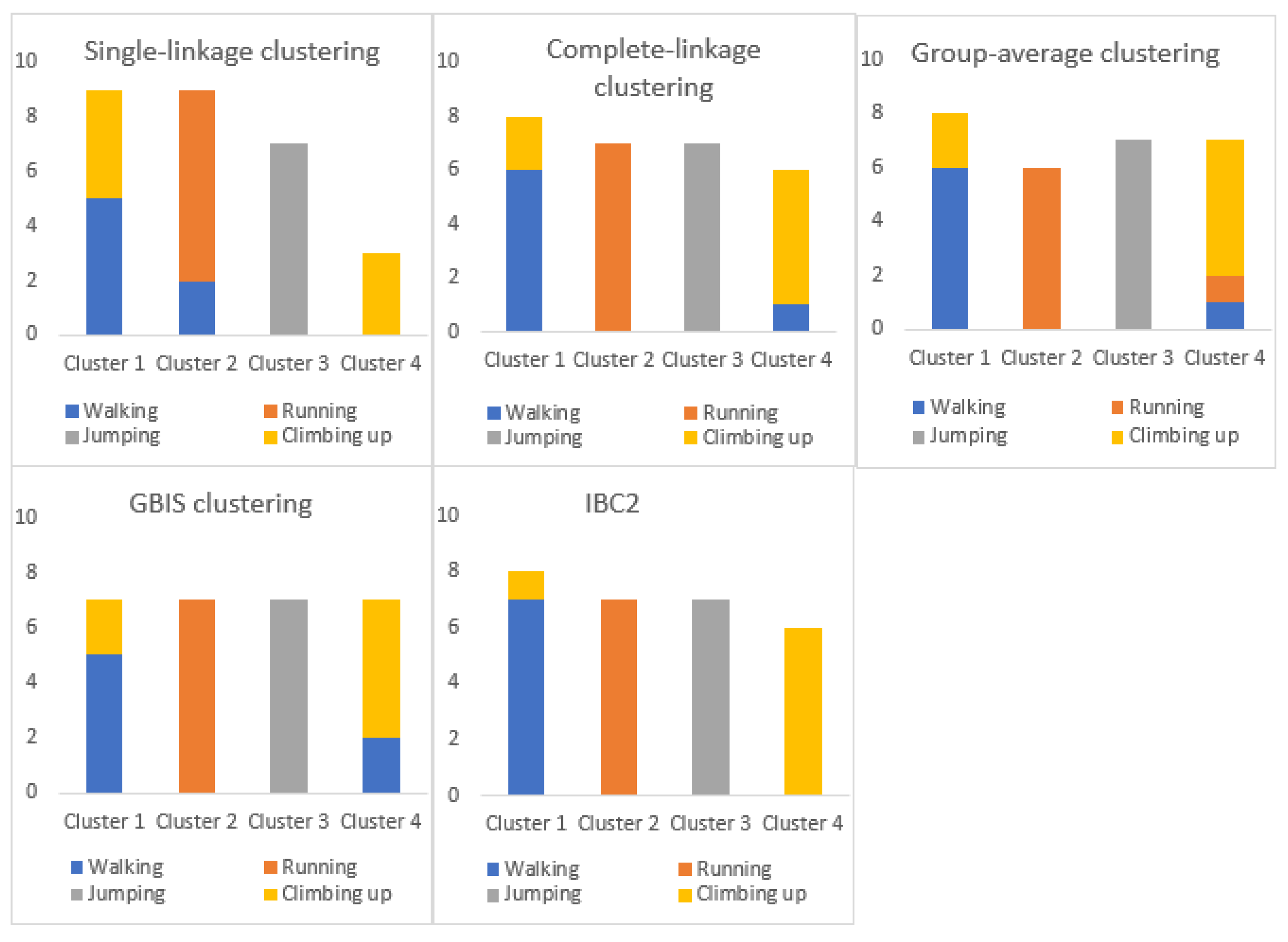
To assess the performance of the novel algorithm, the following graph-based algorithms: single-link, complete-link, group-average agglomerative clustering algorithms [8] and clustering algorithm for graph-based image segmentation (GBIS) [6] are applied on the obtained graphs, in a case when the number of clusters is given beforehand. Comparative clustering results can be seen in Figure 2 and Figure 3. Comparative results of clustering evaluation can be seen in

Table 8. Comparing evaluation parameters using CMU-MMAC database.

	T	RI	P	R	F
Single-linkage clustering algorithm	65.22%	0.802	0.535	0.691	0.603
Complete-linkage clustering algorithm	91.30%	0.913	0.780	0.836	0.807
Group-average clustering algorithm	82.61%	0.854	0.661	0.673	0.667
GBIS clustering algorithm	82.61%	0.834	0.607	0.673	0.638
IBC2 algorithm	95.65%	0.960	0.909	0.909	0.909

and

Table 9. Comparing evaluation parameters using RealWorld data set.

	T	RI	P	R	F
Single-linkage clustering algorithm	67.86%	0.852	0.646	0.738	0.689
Complete-linkage clustering algorithm	89.29%	0.913	0.800	0.810	0.805
Group-average clustering algorithm	85.71%	0.881	0.729	0.738	0.733
GBIS clustering algorithm	85.71%	0.899	0.762	0.762	0.762
IBC2 algorithm	96.43%	0.966	0.918	0.929	0.923

.

6. Discussion

Algorithms for automatic human activity recognition are, for the most part, intended to analyze types of activities that are relatively simple and significantly different from each other, including body postures, simple task-oriented and fundamental behaviors (e.g., sitting, standing, walking, running, swimming, dressing, walking upstairs, walking downstairs, clapping, waving etc.) [3]. Contrary to that, the described algorithm allows the recognition of given complex actions that are not precisely defined. Specifically, different human subjects perform the same type of activity in different ways (e.g., preparing a dish without precise recipe), i.e., individual segments of a complex action are quite different or are performed in a different order. Additionally, different types of complex actions can have the same segments. The presented approach enables successful clustering of such complex human activities.

First, the performance of the novel IBC1 algorithm is analyzed. In Table 2, the results of complex human activities (CMU-MMAC database) clustering are presented. When discussing these results, it can be seen that 23 subject–activity pairs are grouped in six clusters, relate to four ground truth clusters. All four required clusters are formed, containing 20 of 23 pairs, with the Accuracy of formed clusters $T=86.96\%$, with only one false positive. Satisfactory clustering results are confirmed by the evaluation parameters shown in Table 4: Rand Index $RI=0.941$, precision $P=0.976$, recall $R=0.745$ and balanced F-measure $F=0.845$. In IBC1 of Figure 1, the results of fundamental human activities (RealWorld data set) are presented. Twenty-eight subject–activity pairs are grouped in seven clusters, which may appear as significantly more than the four ground truth clusters. However, 25 of 28 pairs are correctly clustered in four clusters, and there are no false positives. All four required clusters are formed with the Accuracy of formed clusters $T=89.29\%$. The satisfying clustering results are confirmed by the evaluation parameters shown in Table 6: Rand Index $RI=0.955$, precision $P=1$, recall $R=0.798$ and balanced F-measure $F=0.888$. The performance of the proposed algorithm is satisfactory on both data sets. Significance of this algorithm is confirmed by, above all, good results of clustering complex human activities.

Furthermore, the performance of the IBC2 algorithm is discussed. For a more thorough evaluation, the following graph-based algorithms: single-link, complete-link, group-average agglomerative clustering algorithms [8] and clustering algorithm for graph-based image segmentation (GBIS) [6], are tested on same samples, in a case when the number of clusters is given beforehand. Comparative results, in the case of complex human activities (CMU-MMAC database) are displayed in Figure 2. It can be concluded that by applying all the algorithms, all four clusters are formed, except in a case with the single-link clustering algorithm. Comparative evaluation results of clustering are displayed in Table 8. The best evaluation results by all parameters are obtained for IBC2 algorithm: The Accuracy of formed clusters $T=95.65\%$, Rand Index $RI=0.960$, precision $P=0.909$, recall $R=0.909$ and balanced F-measure $F=0.909$. Comparative results, in the case of fundamental human activities (RealWorld data set), are illustrated in Figure 3. The conclusion is that by applying all the algorithms all four clusters are formed, except for single-link clustering algorithm, which tends to merge clusters. The best results of all evaluation parameters are obtained for IBC2 algorithm. The Accuracy of formed clusters $T=96.43\%$, Rand Index $RI=0.966$, precision $P=0.918$, recall $R=0.929$ and balanced F-measure $F=0.923$.

To complete comparative analysis, gained results are compared with the results obtained by two different methods used to cluster human activities. According to review [15], most used methods are K-means, and Sub-clustering. In the same review, most significant results gained by aforementioned methods is presented, for each used dataset. The best results published in journals are presented in

Table 10. Comparing methods.

Method	Dataset	$\mathbf{RI}$	References
	VanKasteren	0.872	[16]
	WISDM	0.710	[17]
K-means	Liara	0.860	[18]
	Opportunity	0.868	[19]
	MHealth	0.786	[20]
	UCI HAR	0.794	[21]
	VanKasteren	0.894	[22]
Sub-clustering	Casas Aruba	0.898	[23]
	Casas Kyoto	0.891	[9]
IBC2	RealWorld	0.966

.

The proposed method with IBC2 algorithm gives the best clustering results rated by the Rand Index.

Most clustering algorithms are based solely on the distances between the pair of points, or on the connectivity. The proposed IBC1 algorithm combines these two principles. Furthermore, a metric is not required. Its principal characteristic is capacity to analyze graphs with overlapping clusters, as well as with significant inter-cluster similarities. High in time complexity for many data points is a disadvantage to this algorithm. IBC2 algorithm is inefficient when the number of points per cluster is uneven.

7. Conclusions

With insight into the results obtained by novel algorithms, it can be concluded that they are immensely satisfactory, particularly when the number of clusters is known. The percentages of given cluster vertices belonging to the corresponding formed clusters are $T=86.96\%$ (CMU-MMAC database), $T=89.29\%$ (RealWorld data set) with no prior assumption of the number of clusters; that is, $T=95.65\%$ (CMU-MMAC database), $T=96.43\%$ (RealWorld data set) when the number of clusters is given beforehand.

In further research it would be interesting to find answers to the following questions:

• Would using of new features derived from the original features (e.g., velocity and relative position can be derived from acceleration data)or using more sensors placed on different body parts of subjects, yield better results?
• How to find a method for determining the appropriate percentage value of intruders, in unsupervised scenario?

These issues will be addressed in further work.

References

- Avci, A.; Bosch, S.; Marin-Perianu, M.; Marin-Perianu, R.; Havinga, P. Activity Recognition Using Inertial Sensing for Healthcare, Wellbeing and Sports Applications: A Survey. In Proceedings of the 23rd International Conference on Architecture of Computing Systems 2010, Hannover, Germany, 22–25 February 2010; pp. 1–10. [Google Scholar]
- Hussain, Z.; Sheng, M.; Zhang, W.E. Different Approaches for Human Activity Recognition: A Survey. arXiv 2020, arXiv:1906.05074. [Google Scholar]
- Jobanputra, C.; Bavishi, J.; Doshi, N. Human Activity Recognition: A Survey. Procedia Comput. Sci. 2019, 15, 698–703. [Google Scholar] [CrossRef]
- Sousa Lima, W.; Souto, E.; El-Khatib, K.; Jalali, R.; Gama, J. Human activity recognition using inertial sensors in a smartphone: An overview. Sensors 2019, 19, 3213. [Google Scholar] [CrossRef] [PubMed] [Green Version]
- Vanneste, P.; Oramas, J.; Verelst, T.; Tuytelaars, T.; Raes, A.; Depaepe, F.; Noortgate, W. Computer Vision and Human Behaviour, Emotion and Cognition Detection: A Use Case on Student Engagement. Mathematics 2021, 9, 287. [Google Scholar] [CrossRef]
- Felzenszwalb, P.F.; Huttenlocher, D.P. Efficient Graph-Based Image Segmentation. Int. J. Comput. Vis. 2004, 59, 167–181. [Google Scholar] [CrossRef]
- Li, Y.; Wu, H. A Clustering Method Based on K-Means Algorithm. Phys. Procedia 2012, 25, 1104–1109. [Google Scholar] [CrossRef] [Green Version]
- Manning, C.; Raghavan, P.; Schutze, H. Introduction to Information Retrieval; Cambridge University Press: Cambridge, UK, 2008; Chapter 17. [Google Scholar]
- Yang, Y.; Zheng, K.; Wu, C.; Niu, X.; Yang, Y. Building an effective intrusion detection system using the modified density peak clustering algorithm and deep belief networks. Appl. Sci. 2019, 9, 238. [Google Scholar] [CrossRef] [Green Version]
- Gnjatović, M.; Nikolić, V.; Joksimović, D.; Maček, N.; Budimirović, N. An Approach to Human Activity Clustering using Inertial Measurement Data. In Proceedings of the X International Scientific Conference Archibald Reiss, Belgrade, Serbia, 18–19 November 2020. [Google Scholar]
- Schimke, S.; Vielhauer, C.; Dittmann, J. Using adapted Levenshtein distance for on-line signature authentication. In Proceedings of the 17th International Conference on Pattern Recognition, ICPR 2004, Cambridge, UK, 26–26 August 2004; Volume 2, pp. 931–934. [Google Scholar]
- De la Torre, F.; Hodgins, J.; Montano, J.; Valcarcel, S.; Forcada, R.; Macey, J. Guide to the Carnegie Mellon University Multimodal Activity (CMU-MMAC) Database; Tech. Report CMU-RI-TR-08-22; Robotics Institute, Carnegie Mellon University: Pittsburgh, PA, USA, 2009. [Google Scholar]
- Human Activity Recognition. Available online: https://sensor.informatik.uni-mannheim.de/ (accessed on 20 March 2021).
- Levenshtein, V.I. Binary codes capable of correcting deletions, insertions, and reversals. Cybern. Control Theory 1966, 10, 707–710. [Google Scholar]
- Ariza Colpas, P.; Vicario, E.; De-La-Hoz-Franco, E.; Pineres-Melo, M.; Oviedo-Carrascal, A.; Patara, F. Unsupervised Human Activity Recognition Using the Clustering Approach: A Review. Sensors 2020, 20, 2702. [Google Scholar] [CrossRef] [PubMed]
- Marimuthu, P.; Perumal, V.; Vijayakumar, V. OAFPM: Optimized ANFIS using frequent pattern mining for activity recognition. J. Supercomput. 2019, 75, 5347–5366. [Google Scholar] [CrossRef]
- Chetty, G.; Yamin, M. Intelligent human activity recognition scheme for eHealth applications. Malays. J. Comput. Sci. 2015, 28, 59–69. [Google Scholar]
- Soulas, J.; Lenca, P.; Thépaut, A. Unsupervised discovery of activities of daily living characterized by their periodicity and variability. Eng. Appl. Artif. Intell. 2015, 45, 90–102. [Google Scholar] [CrossRef]
- Wen, J.; Zhong, M. Activity discovering and modelling with labelled and unlabelled data in smart environments. Expert Syst. Appl. 2015, 42, 5800–5810. [Google Scholar] [CrossRef]
- Wang, S.; Li, M.; Hu, N.; Zhu, E.; Hu, J.; Liu, X.; Yin, J. K-means clustering with incomplete data. IEEE Access 2019, 7, 69162–69171. [Google Scholar] [CrossRef]
- Boddana, S.; Talla, H. Performance Examination of Hard Clustering Algorithm with Distance Metrics. Int. J. Innov. Technol. Explor. Eng. 2019, 9, 172–178. [Google Scholar]
- Caleb-Solly, P.; Gupta, P.; McClatchey, R. Tracking changes in user activity from unlabelled smart home sensor data using unsupervised learning methods. Neural Comput. Appl. 2020, 32, 12351–12362. [Google Scholar]
- Patel, A.; Shah, J. Sensor-based activity recognition in the context of ambient assisted living systems: A review. J. Ambient Intell. Smart Environ. 2019, 11, 301–322. [Google Scholar] [CrossRef]
Figure 1.
Clustering results obtained by IBC1 and IBC2 algorithms, using RealWorld data set.
Figure 2.
Comparing clustering results, when the number of clusters is given beforehand, using CMU-MMAC database.
Figure 3.
Comparing clustering results, when the number of clusters is given beforehand, using RealWorld data set.