
Purcell’s Three-Link Swimmer: Assessment of Geometry and Gaits for Optimal Displacement and Efficiency


Industrial Engineering School, University of Extremadura, 06006 Badajoz, Spain
*
Author to whom correspondence should be addressed.
Mathematics 2021, 9(10), 1088; https://doi.org/10.3390/math9101088
Submission received: 9 April 2021
/
Revised: 1 May 2021
/
Accepted: 6 May 2021
/
Published: 12 May 2021
(This article belongs to the Special Issue Models, Methods, and Materials for Untethered Swimming Robots at Low Reynolds Number)
Abstract
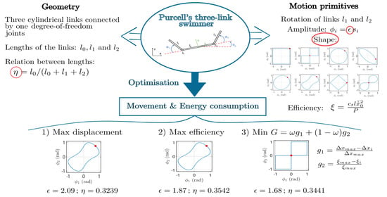
:This paper studies the displacement and efficiency of a Purcell’s three-link microswimmer in low Reynolds number regime, capable of moving by the implementation of a motion primitive or gait. An optimization is accomplished attending to the geometry of the swimmer and the motion primitives, considering the shape of the gait and its amplitude. The objective is to find the geometry of the swimmer, amplitude and shape of the gaits which make optimal the displacement and efficiency, in both an individual way and combined (the last case will be referred to as multiobjective optimization). Three traditional gaits are compared with two primitives proposed by the authors and other three gaits recently defined in the literature. Results demonstrate that the highest displacement is obtained by the Tam and Hosoi optimal velocity gait, which also achieves the best efficiency in terms of energy consumption. The rectilinear and Tam and Hosoi optimal efficiency gaits are the second optimum primitives. Regarding the multiobjective optimization and considering the two criteria with the same weight, the optimum gaits turn out to be the rectilinear and Tam and Hosoi optimal efficiency gaits. Thus, the conclusions of this study can help designers to select, on the one hand, the best swimmer geometry for a desired motion primitive and, on the other, the optimal method of motion for trajectory tracking for such a kind of Purcell’s swimmers depending on the desired control objective.
1. Introduction
Advances in micro- and nanotechnology have promoted the manufacturing of new miniature biomimetic artificial devices inspired by biological systems. New applications emerge due to their ability to access to small spaces at the microscale, such as perform medical procedures in a minimally invasive way, deliver drugs with high precision, and sensing towards diagnosis and monitoring [1,2,3,4]. In this sense, understanding hydrodynamics at the microscale is crucial, which implies navigating in low Reynolds number () regime where viscous forces predominate over inertial ones. In this regime, the study of microswimmer dynamics acquires an important role on understanding the motion and finding new ways to propel these swimmers.
Mainly, two ways of propulsion at low regime can be distinguished [5]. On the one hand, the movement can be obtained by performing a unidirectional body motion, deployed by a rotating corkscrew and based on the movement of prokaryotic cells or bacteria [6]. On the other hand, flexible flagellums of eucaryotic cells have inspired the movement through planar waveforms, leading to the study of different waveforms for propulsion [7,8,9,10] and design of prototypes [11,12]. In this respect, Purcell introduced the so-called Purcell’s three-link swimmer [5], composed of three links attached by one degree-of-freedom joints and defined as the simplest swimmer that could implement a gait or motion primitive within a low flow and manage to move a certain distance. It must be said that there are other types of Purcell’s swimmers depending on the number of links that they are made of (widely called N-link swimmers) [13,14].
Concerning the Purcell’s three-link swimmer, several authors already studied its dynamics comparing the displacement obtained through the implementation of traditional primitives and estimating a coefficient of efficiency based on the energy consumption of the joints [15]. Other works study the dynamics of a 3D model and provide new gaits [16], while others analyze the dynamics of the generalized case of N-link and try to approximate it to a sperm cell swimmer [13]. Regarding the motion primitives, methods for designing new motion primitives have been reported in [14,17,18,19], providing the definition and implementation of different gaits, while other works analyze the symmetries of the Purcell’s three-link swimmers and their effect on generating gaits with particular symmetries in order to achieve a desired net motion [20]. These symmetries allowed to define other stroke sequences, represented as a Fourier Series, which provide optimal efficiency and velocity of the swimmer [21]. Finally, the controllability of the Purcell’s swimmers was studied in [13,14,16,22] and experimental trajectory tracking was addressed in [18,23]. Although considerable work has been done in this field, the defined gaits have not been compared among them, nor any study involving the displacement and efficiency has been carried out with all the motion primitives. In addition, the parameters that influence the movement of Purcell’s swimmer have barely been analyzed.
This work aims to solve these research gaps offering a novel comparative study between gaits in terms of displacement and efficiency towards doing optimal both the geometric design and the trajectory tracking in future works.
This work aims to solve this research gaps offering a novel comparative study between gaits with the objective of optimizing the displacement and efficiency towards the implementation of an optimal trajectory tracking and the design of a prototype in future works. The study focuses on three aspects: the shape and amplitude of the motion primitives, and the swimmer geometry. With the purpose of analyzing the performance from different viewpoints, displacement and efficiency of the Purcell’s three-link microswimmer are reported here in two different ways, namely separately and altogether, this last case by a multiobjective optimization. Regarding the motion primitives, this work proposes two new gaits and compares them with three traditional ones, already studied in the references [13,14,15,16,18,20], and other three gaits defined by other authors [19,21]. The results of this study will provide the optimal primitive along with its best amplitude and geometry of the swimmer for achieving optimal displacement, optimal efficiency and minimizing a multiobjective function. A preliminary work can be found in [24], where the displacement and efficiency were calculated for different primitives, amplitudes and geometries, although these variables were not analyzed together.
The document is organized as follows. Section 2 recalls the environment properties and the hydrodynamics related to low regime, based on the Navier–Stokes equations, as well as the basis of the resistive force theory (RFT). Section 3 addresses the dynamics of Purcell’s three-link swimmers and introduces the gaits analyzed in this work. The optimization of displacement and efficiency is carried out in Section 4, where the two criteria are calculated depending on the shape of the gait, its amplitude, and the geometry of the swimmer. The main conclusions of this work are drawn in Section 5.
2. Background
This section describes the hydrodynamics in the microscale and the estimation of drag forces for the Purcell’s swimmer.
2.1. Environment Properties
Prior to the study of the movement of Purcell’s three-link swimmer, some hydrodynamics concepts are introduced to understand the movement at the microscale.
A moving fluid is characterized by , which determines the influence of viscous and inertial forces through the expression:
where v and l are the maximum velocity and a characteristic dimension of the flow, respectively, and and are the density and the dynamic viscosity of the fluid, respectively. This expression is appropriate for a Newtonian fluid, which dynamic viscosity is constant for every conditions.
Due to the dimensions of ducts and objects, the microscale is characterized by a low regime, which is called slow viscous flow and implies that the viscous forces are dominant while inertial forces are negligible [25].
On another note, the Navier–Stokes equations are essential for studying the hydrodynamics in a fluid. The expression for a Newtonian and incompressible fluid is [25,26]:
where is the material derivative, defined as . The term represents the inertia effects, is the pressure gradient present in the fluid, represents the diffusion and internal forces, and denotes other external forces.
As stated before, in low regime the inertial forces are negligible, and the Navier–Stokes equations transform into the Stokes equations [25]:
On the other hand, the law of conservation of mass can be applied to any stationary volume element within a flowing fluid [25], resulting in the equation of continuity . For an incompressible fluid, the equation can be simplified to , where is the net rate of flux. This simplification along with the Stokes equations establish the creeping motion equations for low regime [25]. If is small, it is permissible to say that there are no external forces applied to the swimmer and the fluid surrounding it. Thus, the external forces term of Stokes equations can be omitted, and the equations adopt the quasi-static form:
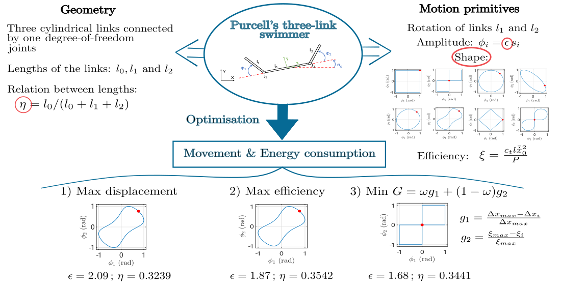
The first consequence of low regime governed by the Stokes equations is the reversibility of a flow: fluid particles follow the same trajectories as a moving body within the fluid, which implies that a swimmer moving to a position and then returning by reversing the same sequence of shapes does not produce net displacement of the swimmer. This was first introduced by Purcell through the ‘scallop theorem’ [5], and consequently, a non-reciprocal motion has to be performed. The difference between reciprocal and non-reciprocal motion applied to a Purcell’s three-link swimmer is illustrated in Figure 1. The selection of an optimal non-reciprocal sequence is crucial for the Purcell’s three-link swimmer in the environment under study, as it has been proved that the net displacement only depends on the geometrical sequence of shape [27].
2.2. Drag Forces by Resistive Force Theory
In addition to the non-reciprocal motion, a moving body within a fluid needs to compensate the reactions opposing the direction of movement to generate a net displacement. These reactions are drag forces and appear longitudinal and tangentially to the direction of displacement [28].
The estimation of drag forces in low regime was studied by several authors, leading to the definition of theories and methods that apply different conditions to the object under study (see e.g., [29] and references therein). The main theories applied to the Purcell’s swimmer are RFT and the slender body theory (SBT). The choice of one or the other is explained hereunder.
First, RFT estimates the drag forces acting on a slender body proportionally to its instantaneous velocity relative to the fluid and the drag coefficients, which are strictly defined by the geometry of the body and the viscosity of the fluid [28,30]. Conversely, SBT approximates the effects of a solid within a flow by a distribution of singularities, taking advantage of the slenderness of the body [31,32,33,34,35,36]. RFT and SBT were compared in [37] and the conclusions pointed out that the results obtained by RFT are consistent with those obtained by SBT in the case that no cell body is attached to the end of the body or if it is of small diameter (hence, it does not affect to the results). This conclusion leads to the application of RFT in the present work, as it is sufficient and generates consistent results, also avoiding the computational efforts of executing SBT analysis. The fundamentals of RFT are introduced hereunder.
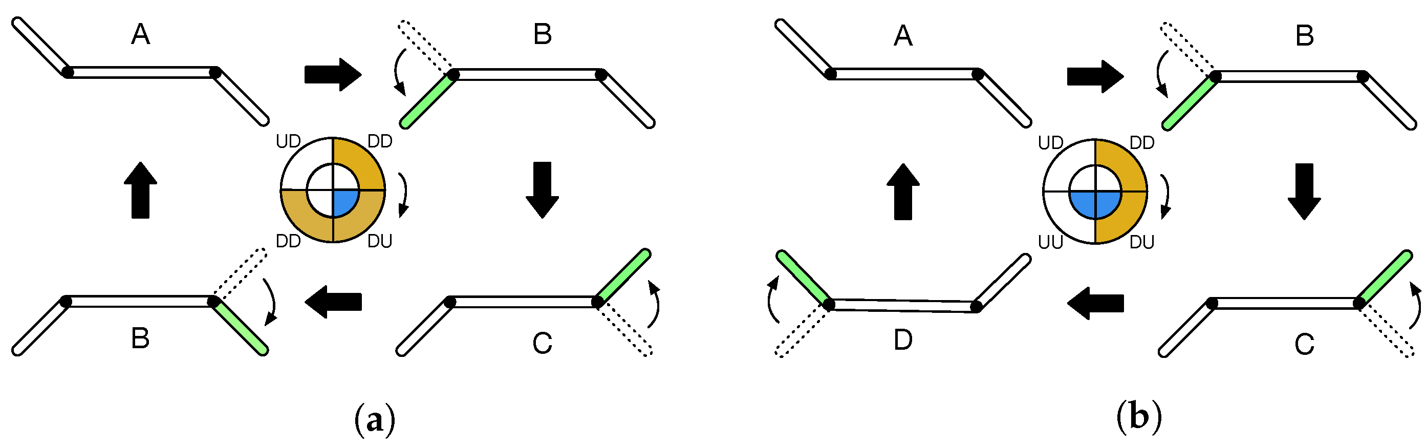
Consider an infinitesimal element of length belonging to a slender body in an incompressible and low fluid. RFT establishes that the tangential and normal reactions of the fluid depend on the drag coefficients ( and , respectively), on the velocity of the object in the direction of X or Y axis ( or ), and on the inclination angle of with respect to the horizontal (). Three situations may be differentiated here: the body moves in the X axis, in the Y axis, and a combination of velocities in both axis.
The reactions applied to the infinitesimal element when the body is moving with a velocity are illustrated in Figure 2a, being and the tangential and normal reactions of the fluid. A similar situation is found when the body moves in the Y axis (Figure 2b). Depending on the direction of the swimmer velocity, the forces of the infinitesimal element are given by [28]:
When the motion is produced by a combination of velocities in X and Y directions (Figure 2c), the total forces acting normally and tangentially to the infinitesimal element are:
Details are given in [38]. The resultant forward thrust in X and Y directions is given by:
being and unit vectors in X and Y directions, respectively. The total drag force applied to an infinitesimal element is the sum of forces and . The torque exerted due to the calculated reactions, denoted as , can be estimated through the cross product of and , being the position of the infinitesimal element from the origin. In accordance with the above equations, the element can only exert a positive forward thrust if and [38].
The drag force and torque applied to a complete segment can be estimated by integrating the force and torque applied to through the total length of the segment ():
3. Purcell’s Three-Link Swimmer
In this section, the geometry and dynamics of the Purcell’s three-link swimmer are introduced, as well as the motion primitives.
3.1. Geometry
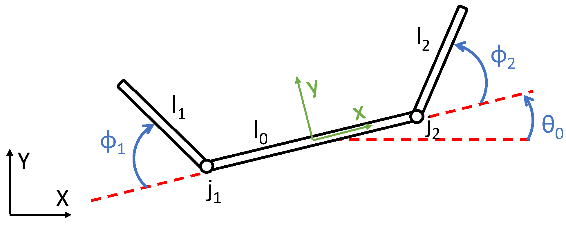
The Purcell’s three-link swimmer consists of three links connected by one degree-of-freedom joints. In this work, the links are supposed cylindrical although another geometry can be considered. The assessment of the swimmer’s dynamics developed in this section takes as a reference the scheme shown in Figure 3.
The lengths of the links are , and , while the rotary joints are designated as and . The lateral links are supposed of equal length () and a ratio is defined to relate the lengths of the links (, being l the total length of the swimmer). Regarding the angular positions of the links, represents the angular position of the ith link with respect to X axis of the global reference frame. The rotation of the lateral links is determined by a motion primitive or gait, which defines the angles and with respect to the body-fixed reference frame . The relations between the angular position and the gait angles are and . The position of the center of ith link is defined as .
3.2. Dynamics
Next, the displacement of the central (or base) link of Purcell’s three-link swimmer will be estimated. First, the planar and angular position of the three links must be analyzed. The movement of links and with respect to the central link is completely defined by angles and , while the position of the base link with respect to the global reference frame is unknown, designated as .
The position of the lateral links with respect to the central link can be easily estimated as follows:
The position can be derived and an expression is obtained, associating the linear and angular velocities of the links (), the linear and angular velocities of the central link (), and the angular velocities of the lateral links with respect to the body-fixed reference frame (). This relation can be written in matrix form, achieving the following expression [15,17,20]:
Matrices and are given in the reference [17] and depend on the link whose velocity is being calculated. The total drag forces and torque applied to the ith link can be calculated through RFT [15], considering , being the radius of the ith link. The following matrix expression is achieved:
where and is called the resistance tensor. The total drag forces acting on the swimmer’s body (denoted as ) are the summation of the forces applied to each link, and the total torque can be estimated by:
where and are the positions of the jth joint and the ith link with respect to the global reference frame, respectively; and is a unit vector in Z direction. According to a Stokes’ flow, a quasi-static motion is assumed; thus, the swimmer is in static equilibrium and the total drag forces and torques acting on the swimmer’s body are [15,17,20]. Substituting into (14) results in:
3.3. Motion Primitives
As a consequence of the reversibility of the flow in low regime, a non-reciprocal motion must be performed towards a net displacement of the swimmer, which can be fulfilled by the application of a motion primitive or gait. As above-mentioned, a gait determines the movement of links and through the angles and . The definition of a gait has been considered to be as follows:
where and are the angles with unitary amplitude, and is the gait amplitude. The shape of a motion primitive determines the displacement reached by the Purcell’s swimmer, so the analysis of different gaits plays a key role to be able to choose the most appropriate.
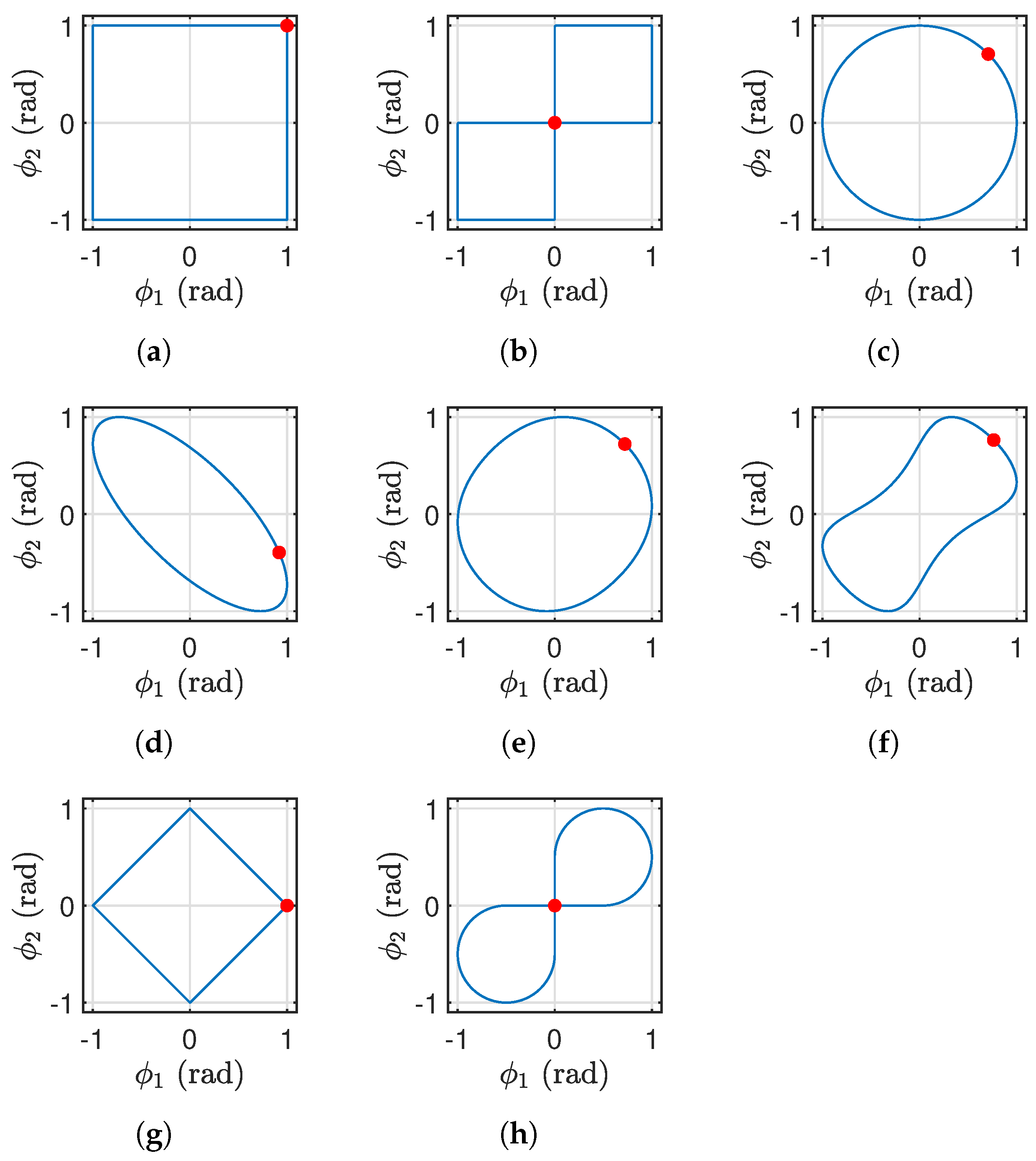
The gaits analyzed in this work are shown in Figure 5 and have been selected following the criteria found in the literature. The square gait is the most common primitive [13,14,15,20,21], followed up by a figure–eight shape (called rectilinear henceforth) [16,18,20] and circular [15]. The gaits in the second row of Figure 5 have been defined in [19,21] as optimal gaits, while the remaining motion primitives are proposed by the authors and were defined by inspiration from the others, and whose definition can be found in Appendix A.
These gaits are divided into two types: consecutive (Figure 5a,b) and simultaneous (the rest). The consecutive gaits are characterized by an alternate movement of the links, i.e., only one link is moving at once. On the other hand, the simultaneous gaits are defined by links constantly moving.
Despite every gait has two versions depending on the direction followed by the angles (clockwise or counterclockwise), it has been proved that the net displacement does not depend on the direction of the gait. In fact, the displacements achieved are identical in magnitude but opposite in sign. It is important to remark that motion primitives in Figure 5 only produce net movement in X axis, thus, displacement in this direction will be studied further on.
4. Optimization of Displacement and Efficiency According to the Shape and Amplitude of the Gaits and the Geometry of the Swimmer
This section presents the results of a comparative study in which the variables to optimize are the displacement of the swimmer, solving the differential Equation (16), and the energy consumption of the joints through a coefficient of efficiency (defined further on). The latter has been considered in this work since the implementation of a gait may achieve the highest displacement while increases the energy consumption, and this must be taken into consideration, especially for trajectory tracking.
The parameters that may affect the displacement of the swimmer are the gait amplitude (), the relation between lengths of the links (), the total length of the swimmer (l), the radius of the links (a), the gait period (), and the viscosity of the fluid (). The displacement varying these parameters is plotted in Figure 6. As a resume, the radius, the gait period and the viscosity do not influence the displacement (Figure 6d–f), considering the range of values of the figure, which have been chosen as the most suitable ones in the scale where the swimmer would navigate. On the other hand, the displacement and the total length of the swimmer have a proportional relation (Figure 6c), which implies that the longer the swimmer, the higher the achieved displacement. Finally, the gait amplitude and the relation between lengths of the links have a major impact on the displacement, and thus, have been considered in the comparative study along with the shape of the gait. The gait amplitude is within the range due to physical restrictions and to extend the limits considered in [24].
The results included in the following subsections have been obtained with MATLAB® and were calculated considering a millimeter size of the robot ( mm). The radius of the links is also assumed small ( mm), and the fluid in which the swimmer would navigate is a silicone oil characterized by a viscosity kg/(m·s), meeting the requisites of low regime and selected for future in-lab experiments.
4.1. Optimal Displacement
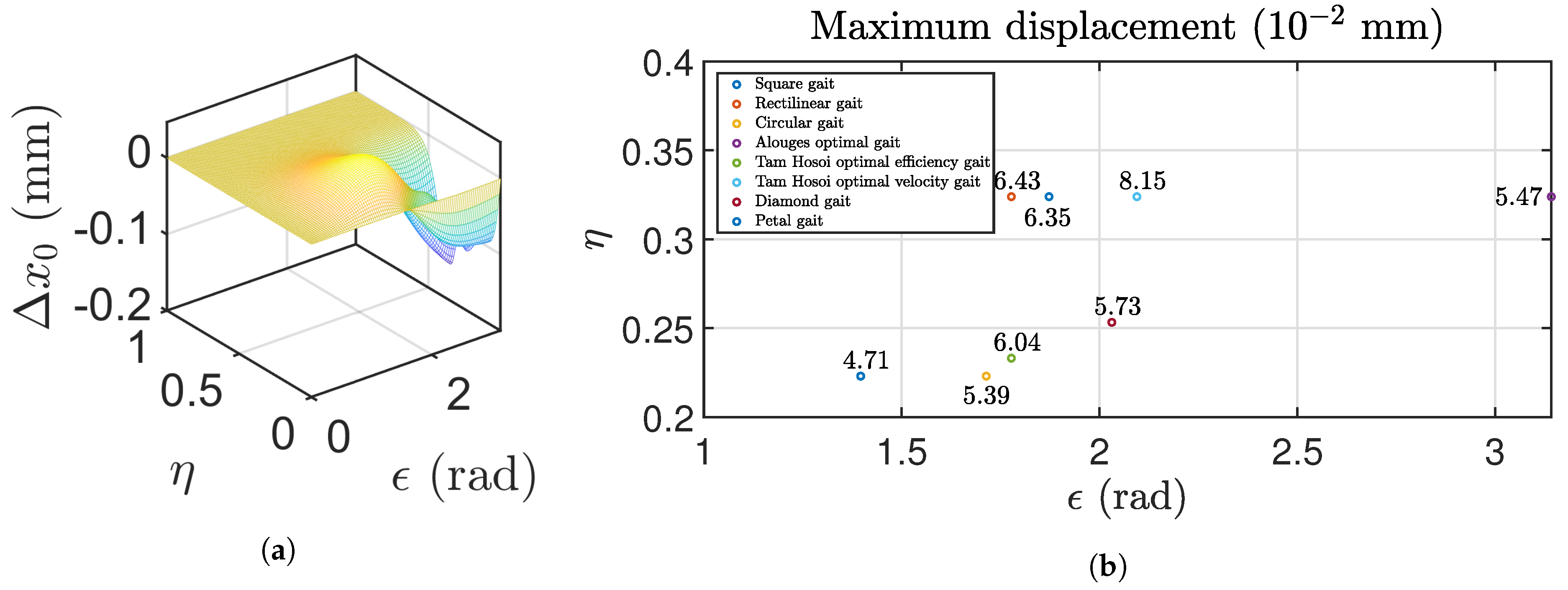
The first parameter to be analyzed is the displacement of the swimmer. The calculations have been carried out varying both the gait amplitude and the relation between lengths of the links, obtaining a data array that can be plotted in 3D as shown in Figure 7a. From these data, the maximum values of displacement can be extracted, which are tabulated in Table 1 in order of decreasing displacement. For additional information and to resume the results, the data from Table 1 is also displayed in Figure 7b.
As it can be extracted from the results, the maximum displacement is achieved for values of 1.4 rad 2.1 rad and . However, there is a maximum out of these limits, corresponding to the Alouges optimal gait from [19], which reaches the maximum value of displacement for rad. It should be evaluated if this gait amplitude is possible to be implemented or, due to physical restrictions, such amplitude is not suitable and must be neglected. This gait does not present any other optimal points in the range under study, so the unique optimal displacement corresponds to this point. The amplitude limits should be taken into account to select the most appropriate primitive, as all the analyzed gaits exhibit similar results and achieve the maximum displacement for amplitudes higher than 1.57 rad.
On the other hand, Table 1 provides the Tam and Hosoi optimal velocity gait from [21] as the optimal one taking into account the displacement, as the Purcell’s swimmer can reach a distance of 81.5 μm through the implementation of this gait. The next three gaits in Table 1 present similar displacements around 60 and 65 μm. These primitives are rectilinear, petal and Tam and Hosoi optimal efficiency gait from [21], in order of decreasing displacement. The worst primitive in this case is the square one, providing a displacement of 47 μm. As it can be observed, the first gait reaches two times the displacement of the square gait.
4.2. Optimal Efficiency
Once the displacement has been calculated, the energy consumption of the joints must be taken into consideration to develop a suitable optimization study, as the Purcell’s swimmer may achieve the highest displacement while increases the energy consumption. This is highly important for trajectory tracking and for the choice of the best non-reciprocal motion.
A useful criterion to evaluate the energy consumption versus the displacement achieved is a coefficient of efficiency, which can be estimated for a Purcell’s three-link swimmer as [15,21,31,39]:
being the average velocity of the center of link , and P the average mechanical power deployed by the joints, calculated through [15].
As performed in the previous subsection, the efficiency is calculated varying both the gait amplitude and the relation between lengths of the links. As it can be observed from Figure 6a, the majority of the gaits reaches the highest displacement at a turning point and, from then on, the displacement decreases while the gait amplitude rises. In this work, only positive displacements in X axis are considered, so the values of efficiency that correspond to negative displacement will be neglected.
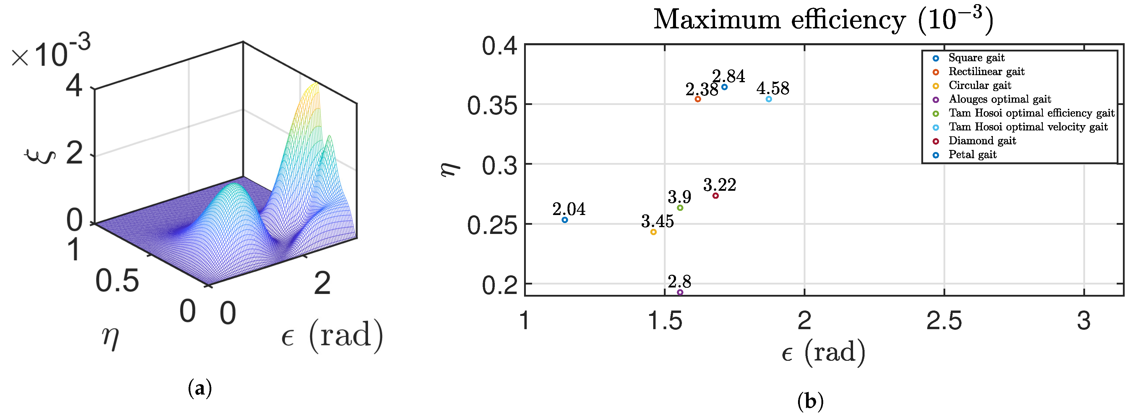
From the data array obtained, the maximum values of efficiency can be extracted, which are tabulated in Table 2 along with their corresponding gait amplitude and relation between lengths of the links. Additionally, Figure 8b shows the same data in a plot. As it can be extracted from this figure, the maximum efficiency is reached for values of 1 rad 2 rad and , which are similar to those of the maximum displacement in the previous section.
Regarding the classification in Table 2, the most efficient primitive matches the one that allows obtaining the highest displacement, i.e., the Tam and Hosoi optimal velocity gait from [21]. The primitive is followed up by the Tam and Hosoi optimal efficiency gait, in the second place, and the circular and diamond primitives, in third and fourth place. The last gait is, again, the square one.
4.3. Multiobjective Optimization
In the previous subsections, separated optimizations have been carried out considering the displacement and the efficiency as the objectives to maximize. In order to complete the study, these two criteria previously defined are considered at the same time through a multiobjective optimization.
The optimization problems can be classified through the number of decision variables, the type of decision variable, the type of objective function, and the form of the problem. If the problem has more than one objective to be satisfied, it is called multiobjective or multicriteria optimization problem. Within the multiobjective optimization methods, the following classification divides the methods into five groups [40,41]:
- Scalar methods: transform the multiobjective problem into a mono-objective problem.
- Interactive methods: sequential processes composed of several iterations.
- Fuzzy methods: involving fuzzy logic.
- Multiobjective methods using metaheuristics: they are stochastic methods, designed to solve difficult optimization problems by means of an intuitive approach.
- Decision aid methods: based on the establishment of an orderly relationship between the different actions or solutions.
The scalar methods will be used in this work, due to their simplicity. Moreover, within the scalar methods, the weighted-sum-of-objective-functions method will be accomplished, in which each criterion or subfunction is associated with a weight and, then, the main objective function is defined as a weighted sum of the objective subfunctions [40]. Usually, the optimization method includes a minimization of the objective function. For that purpose, the new objective function must be defined as follows:
where are the weights associated with each criterion and k is the number of objectives. In this case, the subfunctions are the displacement and efficiency relative errors with respect to their maximum values, defined as:
Combining the above equations and considering , the objective function (19) is:
The last step consists of defining the weight . The optimization can be carried out with the aim of finding the optimal values for the weights, but in this case, both criteria and wish to have the same importance in the multiobjective optimization. Thus, the weights are chosen as .
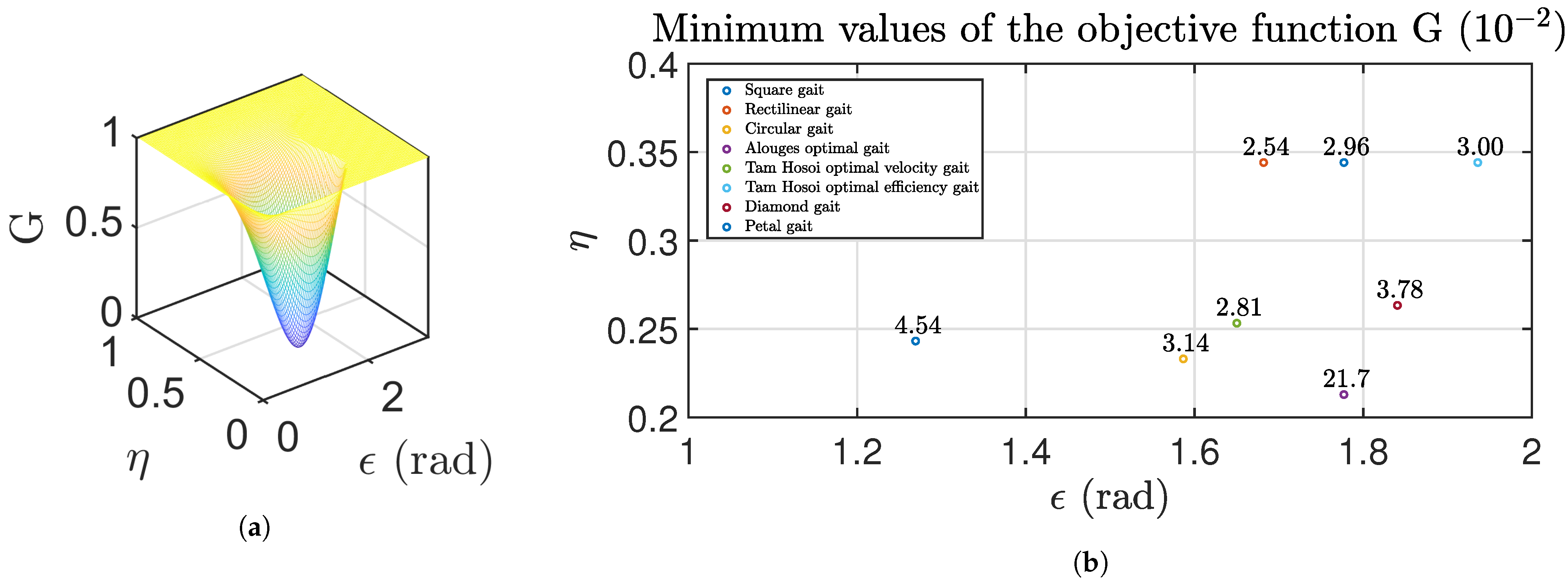
As in the previous analyses, a data array is obtained (plotted in 3D in Figure 9a) and the minimum value of the function can be extracted. Table 3 summarizes the minimum values of along with their corresponding gait amplitude and relation between lengths of the links, being the data sorted in order of increasing function value. The results are also shown graphically in Figure 9b.
The results in Figure 9b show that the primitives are optimal in the range 1.2 rad 2 rad and , similar to the previous criteria of displacement and efficiency. Moreover, considering the results in Table 3, the rectilinear gait is the optimum one, followed up by the Tam and Hosoi optimal efficiency gait in [21], petal gait and Tam and Hosoi optimal velocity gait. The order of the primitives differs from that in previous criteria, as now the Tam and Hosoi optimal velocity gait is not the optimal primitive and the worst primitive is the Alouges optimal gait in [19].
5. Conclusions
This paper has studied the displacement and efficiency of Purcell’s three-link microswimmer in low Reynolds number regime extending the comparative study carried out in [24]. The optimization study has been accomplished attending to the geometry of the swimmer and the motion primitives, focusing on two aspects: the shape of the gait and its amplitude. For this aim, two new gaits have been designed, simulated and compared to three traditional primitives and other three optimal primitives already studied in the references.
Three procedures have been carried out. In the first two of them, the displacement and efficiency have been maximized, while a multiobjective optimization has been performed considering the two previous criteria in terms of error. Common to all the procedures, the data have been estimated varying the amplitude and geometry at the same time.
The results demonstrated that both the maximum displacement and efficiency are achieved for values of gait amplitude between 1 and 2 rad, and relation between lengths of the links () between 0.2 and 0.4. The same occurs with the multiobjective optimization.
In terms of maximum displacement, the best primitive is the Tam and Hosoi optimal velocity gait in [21], followed by the rectilinear and petal gaits, being the petal primitive proposed by the authors. With respect to the maximum efficiency, the Tam and Hosoi optimal velocity gait is also the best one, while the Tam and Hosoi optimal efficiency gait in [21] and the circular one are in third and fourth place. Regarding assigning the same weight to both criteria, the rectilinear gait gives the optimum results, followed by the Tam and Hosoi optimal efficiency gait and the petal gait.
As a conclusion, the results of this study can be useful for selecting the optimal method of motion, with respect to the type of gait, its amplitude and even the swimmer geometry, depending on the desired control objective in trajectory tracking.
Our future works will focus on: (1) designing the optimal control for trajectory tracking of a Purcell’s three-link swimmer, (2) designing and testing experimentally a Purcell’s swimmer prototype, and (3) studying its controllability.
Author Contributions
This work involved all coauthors. C.N.-G. wrote the original draft and contributed to the investigation and the analysis, edited the manuscript and contributed to the illustrations. J.E.T. contributed to the illustrations and the editing. I.T. and B.M.V. conceived the idea, contributed to the editing and supervised all the manuscript. All authors have read and agreed to the published version of the manuscript.
Funding
This work has been supported in part by the Consejería de Economía, Ciencia y Agenda Digital (Junta de Extremadura) under the project IB18109 and the grant “Ayuda a Grupos de Investigación de Extremadura” (no. GR18159), and in part by the European Regional Development Fund “A way to make Europe”.
Institutional Review Board Statement
Not applicable.
Informed Consent Statement
Not applicable.
Data Availability Statement
The data will be available under request.
Acknowledgments
Cristina Nuevo-Gallardo would like to thank University of Extremadura its support through the scholarship “Plan Propio de Iniciación a la Investigación, Desarrollo Tecnológico e Innovación 2019”.
Conflicts of Interest
The authors declare no conflict of interest.
Abbreviations
The following abbreviations are used in this manuscript:
| Re | Reynolds number |
| RFT | Resistive Force Theory |
| SBT | Slender Body Theory |
Appendix A
In this appendix, the definition of the new gaits proposed in this work is provided. These primitives are diamond and petal.
The unscaled angles and for these primitives in their clockwise version are defined as piecewise functions by the following equations:
where is the final time of simulation and the segments are considered of equal duration.
References
- Sitti, M.; Ceylan, H.; Hu, W.; Giltinan, J.; Turan, M.; Yim, S.; Diller, E. Biomedical Applications of Untethered Mobile Milli/Microrobots. Proc. IEEE 2015, 103, 205–224. [Google Scholar] [CrossRef]
- Li, J.; Esteban-Fernández de Ávila, B.; Gao, W.; Zhang, L.; Wang, J. Micro/nanorobots for biomedicine: Delivery, surgery, sensing, and detoxification. Sci. Robot. 2017, 2, eaam6431. [Google Scholar] [CrossRef] [PubMed]
- Medina-Sánchez, M.; Xu, H.; Schmidt, O.G. Micro- and nano-motors: The new generation of drug carriers. Ther. Deliv. 2018, 9, 303–316. [Google Scholar] [CrossRef] [Green Version]
- Soto, F.; Wang, J.; Ahmed, R.; Demirci, U. Medical Micro/Nanorobots in Precision Medicine. Adv. Sci. 2020, 7, 2002203. [Google Scholar] [CrossRef]
- Purcell, E.M. Life at low Reynolds number. Am. J. Phys. 1977, 45, 3–11. [Google Scholar] [CrossRef] [Green Version]
- Silva, J.; Prieto, J.; Tejado, I.; Pérez, E.; Vinagre, B.M. Robots nadadores tipo flagelo bacteriano de pequeñas dimensiones: Desarrollo de prototipos y plataformas de prueba. In Proceedings of the XXXVII Jornadas de Automática, Madrid, Spain, 7–9 September 2016; pp. 740–747. (In Spanish). [Google Scholar]
- Traver, J.E.; Vinagre, B.M.; Tejado, I. Robot nadador tipo flagelo bacteriano plano: Estudio y simulación del mecanismo de propulsión. In Proceedings of the XXXVII Jornadas de Automática, Madrid, Spain, 7–9 September 2016; pp. 1075–1082. (In Spanish). [Google Scholar]
- Traver, J.E.; Tejado, I.; Vinagre, B.M. A Comparative Study of Planar Waveforms for Propulsion of a Joined Artificial Bacterial Flagella Swimming Robot. In Proceedings of the 4th International Conference on Control, Decision and Information Technologies (CoDIT’17), Barcelona, Spain, 5–7 April 2017; pp. 550–555. [Google Scholar]
- Prieto-Arranz, J.; Traver, J.E.; López, M.A.; Tejado, I.; Vinagre, B.M. Study in COMSOL of the generation of traveling waves in an AEF robot by piezoelectric actuation. In Proceedings of the XXXIX Jornadas de Automática, Badajoz, Spain, 5–7 September 2018; pp. 748–755. [Google Scholar]
- Traver, J.E.; Tejado, I.; Prieto-Arranz, J.; Nuevo-Gallardo, C.; Vinagre, B.M. Improved Locomotion of an AEF Swimming Robot Using Fractional Order Control. In Proceedings of the 2019 IEEE International Conference on Systems, Man, and Cybernetics (IEEE SMC 2019), Bari, Italy, 6–9 October 2019; pp. 2559–2564. [Google Scholar]
- Traver, J.E.; Tejado, I.; Nuevo-Gallardo, C.; Prieto-Arranz, J.; López, M.A.; Vinagre, B.M. Evaluating an AEF Swimming Microrobot Using a Hardware-in-the-loop Testbed. In Robot 2019: Fourth Iberian Robotics Conference; Springer: Cham, Switzerland, 2020; pp. 524–536. [Google Scholar]
- Traver, J.E.; Tejado, I.; Nuevo-Gallardo, C.; López, M.A.; Vinagre, B.M. Performance study of propulsion of N-link artificial Eukaryotic flagellum swimming microrobot within a fractional order approach: From simulations to hardware-in-the-loop experiments. Eur. J. Control 2021, 58, 340–356. [Google Scholar] [CrossRef]
- Alouges, F.; DeSimone, A.; Giraldi, L.; Zoppello, M. Self-propulsion of slender micro-swimmers by curvature control: N-link swimmers. Int. J. Non-Linear Mech. 2013, 56, 132–141. [Google Scholar] [CrossRef]
- Giraldi, L.; Martinon, P.; Zoppello, M. Controllability and optimal strokes for N-link microswimmer. In Proceedings of the 52nd IEEE Conference on Decision and Control, Firenze, Italy, 10–13 December 2013; pp. 3870–3875. [Google Scholar]
- Wiezel, O.; Or, Y. Optimization and small-amplitude analysis of Purcell’s three-link microswimmer model. Proc. R. Soc. A Math. Phys. Eng. Sci. 2016, 472, 4–25. [Google Scholar] [CrossRef] [PubMed] [Green Version]
- Kadam, S.; Banavar, R. Geometry of locomotion of the generalized Purcell’s swimmer: Modelling, controllability and motion primitives. IFAC J. Syst. Control 2018, 4, 7–16. [Google Scholar] [CrossRef]
- Wiezel, O.; Or, Y. Using optimal control to obtain maximum displacement gait for Purcell’s three-link swimmer. In Proceedings of the 2016 IEEE 55th Conference on Decision and Control (CDC), Las Vegas, NV, USA, 12–14 December 2016; pp. 4463–4468. [Google Scholar]
- Kadam, S.; Joshi, K.; Gupta, N.; Katdare, P.; Banavar, R.N. Trajectory tracking using motion primitives for the Purcell’s swimmer. In Proceedings of the 2017 IEEE/RSJ International Conference on Intelligent Robots and Systems (IROS), Vancouver, BC, Canada, 24–28 September 2017; pp. 3246–3251. [Google Scholar]
- Alouges, F.; DeSimone, A.; Giraldi, L.; Or, Y.; Wiezel, O. Energy-optimal strokes for multi-link microswimmers: Purcell’s loops and Taylor’s waves reconciled. New J. Phys. 2019, 21, 043050. [Google Scholar] [CrossRef] [Green Version]
- Gutman, E.; Or, Y. Symmetries and gaits for Purcell’s three-link microswimmer model. IEEE Trans. Robot. 2016, 32, 53–69. [Google Scholar] [CrossRef]
- Tam, D.; Hosoi, A.E. Optimal stroke patterns for Purcell’s three-link swimmer. Phys. Rev. Lett. 2007, 98, 068105. [Google Scholar] [CrossRef] [PubMed] [Green Version]
- Kadam, S.; Banavar, R.N. Geometric Controllability of The Purcell’s Swimmer and its Symmetrized Cousin. IFAC-PapersOnLine 2016, 49, 988–993. [Google Scholar] [CrossRef]
- Jaskaran, S.G. Geometric Approaches to Motion Planning for Two Classes of Low Reynolds Number Swimmers. Ph.D. Thesis, The Robotics Institute, School of Computer Science, Carnegie Mellon University, Pittsburgh, PA, USA, 2018. [Google Scholar]
- Nuevo-Gallardo, C.; Traver, J.E.; Tejado, I.; Vinagre, B.M.; Rodríguez, P. Comparative study of gaits and geometry for optimal displacement and efficiency of Purcell’s three-link microswimmers. In Proceedings of the 28nd Seminario Anual de Automática, Electrónica Industrial e Instrumentación, Ciudad Real, Spain, 7–9 July 2021. submitted. [Google Scholar]
- Happel, J.; Brenner, H. Low Reynolds Number Hydrodynamics, 2nd ed.; Martinus Nijhoff Publishers: The Hague, The Netherlands, 1983. [Google Scholar]
- White, F.M. Fluid Mechanics, 7th ed.; Mc Graw-Hill: New York, NY, USA, 2011. [Google Scholar]
- Lauga, E.; Powers, T.R. The hydrodynamics of swimming microorganisms. Rep. Prog. Phys. 2009, 72, 096601. [Google Scholar] [CrossRef]
- Gray, J. The movement of sea-urchin spermatozoa. J. Exp. Biol. 1955, 32, 775. [Google Scholar] [CrossRef]
- Rathore, J.S.; Sharma, N.N. Engineering nanorobots: Chronology of modeling flagellar propulsion. J. Nanotechnol. Eng. Med. 2010, 1, 031001. [Google Scholar] [CrossRef]
- Cox, R.G. The motion of long slender bodies in a viscous fluid. Part 1. General theory. J. Fluid Mech. 1970, 44, 791–810. [Google Scholar] [CrossRef]
- Lighthill, J. Flagellar hydrodynamics. SIAM Rev. 1976, 18, 161–230. [Google Scholar] [CrossRef]
- Johnson, R.E. Slender body theory for Stokes flow and flagellar hydrodynamics. Ph.D. Thesis, California Institute of Technology, Pasadena, CA, USA, 1977. [Google Scholar]
- Johnson, R.E.; Wu, T.Y.T. Hydromechanics of low-Reynolds-number flow. Part 5. Motion of a slender torus. J. Fluid Mech. 1979, 95, 263–277. [Google Scholar] [CrossRef] [Green Version]
- Johnson, R.E. An improved slender-body theory for Stokes flow. J. Fluid Mech. 1980, 99, 411–431. [Google Scholar] [CrossRef]
- Chwang, A.T.; Wu, T.Y.T. Hydromechanics of low-Reynolds-number flow. Part 1. Rotation of axisymmetric prolate bodies. J. Fluid Mech. 1974, 63, 607–622. [Google Scholar] [CrossRef] [Green Version]
- Chwang, A.T.; Wu, T.Y.T. Hydromechanics of low-Reynolds-number flow. Part 2. Singularity method for Stokes flows. J. Fluid Mech. 1975, 67, 787–815. [Google Scholar] [CrossRef] [Green Version]
- Johnson, R.E.; Brokaw, C.J. Flagellar hydrodynamics. A comparison between resistive-force theory and slender-body theory. Biophys. J. 1979, 25, 113–127. [Google Scholar] [CrossRef] [Green Version]
- Gray, J.; Hancock, G.J. The propulsion of sea-urchin spermatozoa. J. Exp. Biol. 1955, 32, 802–814. [Google Scholar] [CrossRef]
- Becker, L.E.; Koehler, S.A.; Stone, H.A. On self-propulsion of micro-machines at low Reynolds number: Purcell’s three-link swimmer. J. Fluid Mech. 2003, 490, 15–35. [Google Scholar] [CrossRef] [Green Version]
- Collette, Y.; Siarry, P. Multiobjective Optimization: Principles and Case Studies, 1st ed.; Decision Engineering; Springer: Berlin/Heidelberg, Germany, 2004. [Google Scholar]
- Méndez-Babey, M. Algoritmos Evolutivos y Preferencias del Decisor Aplicados a Problemas de Optimización Multiobjetivo Discretos. Ph.D. Thesis, Departamento de Ingeniería Mecánica, Universidad de Las Palmas de Gran Canaria, Las Palmas de Gran Canaria, Spain, 2008. (In Spanish). [Google Scholar]
Figure 1.
Types of movement of a Purcell’s three-link swimmer: (a) reciprocal (b) non-reciprocal.

Figure 2.
Fluid reactions applied to an infinitesimal element, defined by RFT: (a) motion in X axis (b) motion in Y axis (c) total drag forces.
Figure 2.
Fluid reactions applied to an infinitesimal element, defined by RFT: (a) motion in X axis (b) motion in Y axis (c) total drag forces.

Figure 3.
General scheme of the Purcell’s three-link swimmer.

Figure 4.
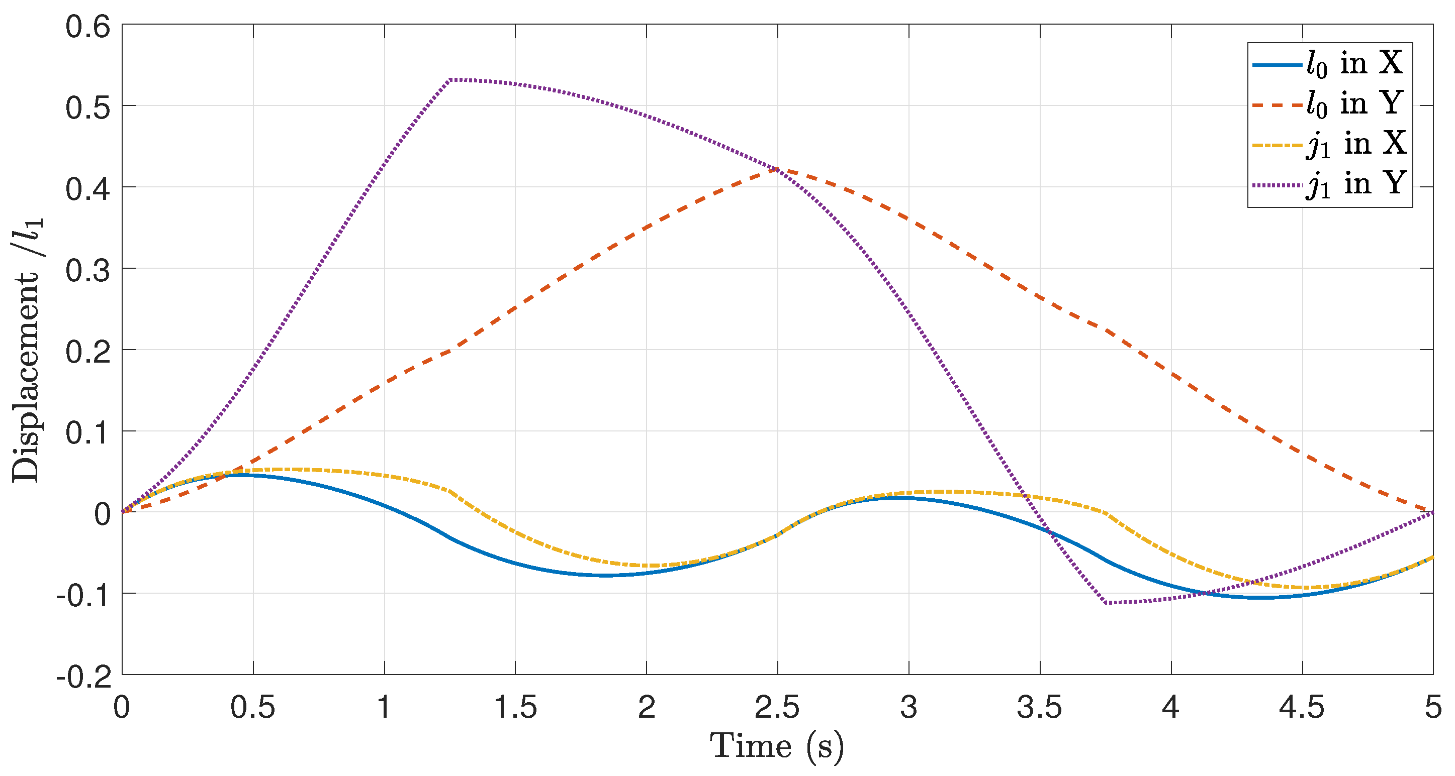
Normalized displacement of the central link () and left joint () of the Purcell’s three-link swimmer in X and Y axis, implementing a square gait with as its amplitude, , and . The results match those presented in [13,39].

Figure 5.
Different gaits applied to the Purcell’s swimmer, with unitary amplitude: (a) square (b) rectilinear (c) circular (d) Alouges optimal gait from [19] (e) optimal efficiency gait from [21] (f) optimal velocity gait from [21] (g) diamond gait (h) petal gait. The coloured circular mark represents the initial point of the gait.

Figure 6.
Displacement of the Purcell’s three-link swimmer depending on several parameters which may influence its movement: (a) amplitude of the gait () (b) relation between lengths of the links () (c) radius of the links (a) (d) total length of the swimmer (l) (e) gait period () (f) viscosity of the fluid ().

Figure 7.
Results for optimal displacement: (a) 3D plot of displacement applying the square gait to the Purcell’s three-link swimmer, (b) maximum values of displacement with their corresponding gait amplitude () and relation between lengths of the links ().
Figure 7.
Results for optimal displacement: (a) 3D plot of displacement applying the square gait to the Purcell’s three-link swimmer, (b) maximum values of displacement with their corresponding gait amplitude () and relation between lengths of the links ().

Figure 8.
Results for optimal efficiency: (a) 3D plot of efficiency applying the square gait to the Purcell’s three-link swimmer, (b) maximum values of efficiency with their corresponding gait amplitude () and relation between lengths of the links ().
Figure 8.
Results for optimal efficiency: (a) 3D plot of efficiency applying the square gait to the Purcell’s three-link swimmer, (b) maximum values of efficiency with their corresponding gait amplitude () and relation between lengths of the links ().

Figure 9.
Results from optimal objective function: (a) 3D plot of the objective function applying the square gait, (b) minimum values of the objective function with their corresponding gait amplitude () and relation between lengths of the links ().
Figure 9.
Results from optimal objective function: (a) 3D plot of the objective function applying the square gait, (b) minimum values of the objective function with their corresponding gait amplitude () and relation between lengths of the links ().


Table 1.
Optimal values of gait amplitude () and relation between lengths of the links () for maximum displacement. The data are sorted in order of decreasing displacement.
Table 1.
Optimal values of gait amplitude () and relation between lengths of the links () for maximum displacement. The data are sorted in order of decreasing displacement.
| Gait | (mm) | ||
|---|---|---|---|
| Tam Hosoi optimal velocity gait | |||
| Rectilinear | |||
| Petal | |||
| Tam Hosoi optimal efficiency gait | |||
| Diamond | |||
| Alouges optimal gait | |||
| Circular | |||
| Square |
Table 2.
Optimal values of gait amplitude () and relation between lengths of the links () for maximum efficiency. The data are sorted in order of decreasing efficiency.
Table 2.
Optimal values of gait amplitude () and relation between lengths of the links () for maximum efficiency. The data are sorted in order of decreasing efficiency.
| Gait | |||
|---|---|---|---|
| Tam Hosoi optimal velocity gait | |||
| Tam Hosoi optimal efficiency gait | |||
| Circular | |||
| Diamond | |||
| Alouges optimal gait | |||
| Petal | |||
| Rectilinear | |||
| Square |
Table 3.
Optimal values of gait amplitude () and relation between lengths of the links () for minimum values of the objective function. The data are sorted in order of increasing function value.
Table 3.
Optimal values of gait amplitude () and relation between lengths of the links () for minimum values of the objective function. The data are sorted in order of increasing function value.
| Gait | |||
|---|---|---|---|
| Rectilinear | |||
| Tam Hosoi optimal efficiency gait | |||
| Petal | 03441 | ||
| Tam Hosoi optimal velocity gait | |||
| Circular | |||
| Diamond | |||
| Square | |||
| Alouges optimal gait |
Publisher’s Note: MDPI stays neutral with regard to jurisdictional claims in published maps and institutional affiliations. |
© 2021 by the authors. Licensee MDPI, Basel, Switzerland. This article is an open access article distributed under the terms and conditions of the Creative Commons Attribution (CC BY) license (https://creativecommons.org/licenses/by/4.0/).
Share and Cite
MDPI and ACS Style
Nuevo-Gallardo, C.; Traver, J.E.; Tejado, I.; Vinagre, B.M. Purcell’s Three-Link Swimmer: Assessment of Geometry and Gaits for Optimal Displacement and Efficiency. Mathematics 2021, 9, 1088. https://doi.org/10.3390/math9101088
AMA Style
Nuevo-Gallardo C, Traver JE, Tejado I, Vinagre BM. Purcell’s Three-Link Swimmer: Assessment of Geometry and Gaits for Optimal Displacement and Efficiency. Mathematics. 2021; 9(10):1088. https://doi.org/10.3390/math9101088
Chicago/Turabian StyleNuevo-Gallardo, Cristina, José Emilio Traver, Inés Tejado, and Blas M. Vinagre. 2021. "Purcell’s Three-Link Swimmer: Assessment of Geometry and Gaits for Optimal Displacement and Efficiency" Mathematics 9, no. 10: 1088. https://doi.org/10.3390/math9101088
Note that from the first issue of 2016, this journal uses article numbers instead of page numbers. See further details here.