
Bremsstrahlung of Light through Spontaneous Emission of Gravitational Waves


Department of Physics, University of Aberdeen, King’s College, Aberdeen AB24 3UE, UK
*
Author to whom correspondence should be addressed.
Symmetry 2021, 13(5), 852; https://doi.org/10.3390/sym13050852
Submission received: 14 April 2021
/
Revised: 7 May 2021
/
Accepted: 8 May 2021
/
Published: 11 May 2021
(This article belongs to the Special Issue Quantum Gravity)
Abstract
:Zero-point fluctuations are a universal consequence of quantum theory. Vacuum fluctuations of electromagnetic field have provided crucial evidence and guidance for QED as a successful quantum field theory with a defining gauge symmetry through the Lamb shift, Casimir effect, and spontaneous emission. In an accelerated frame, the thermalisation of the zero-point electromagnetic field gives rise to the Unruh effect linked to the Hawking effect of a black hole via the equivalence principle. This principle is the basis of general covariance, the symmetry of general relativity as the classical theory of gravity. If quantum gravity exists, the quantum vacuum fluctuations of the gravitational field should also lead to the quantum decoherence and dissertation of general forms of energy and matter. Here we present a novel theoretical effect involving the spontaneous emission of soft gravitons by photons as they bend around a heavy mass and discuss its observational prospects. Our analytic and numerical investigations suggest that the gravitational bending of starlight predicted by classical general relativity should also be accompanied by the emission of gravitational waves. This in turn redshifts the light causing a loss of its energy somewhat analogous to the bremsstrahlung of electrons by a heavier charged particle. It is suggested that this new effect may be important for a combined astronomical source of intense gravity and high-frequency radiation such as X-ray binaries and that the proposed LISA mission may be potentially sensitive to the resulting sub-Hz stochastic gravitational waves.
1. Introduction
The quantum vacuum is a remarkable consequence of the quantum field theory (QFT). To be sure, the quantum electrodynamics (QED) as the first successful QFT has received crucial guidance and support through its quantum vacuum effects including the Lamb shift, Casimir effect, and spontaneous emission.
Although the physical reality of the quantum vacuum seems to contradict the void classical vacuum, it in fact forges essential links between classical and quantum dynamics. The general agreement between the classical emission rate and quantum spontaneous emission rate of electromagnetic (EM) dipole radiations have been well-known at atomic scales (see e.g., [1]). Such an agreement is also clear in the classical cyclotron radiation and the quantum spontaneous emission of the Landau levels [2], in the context of detecting Unruh radiation as a quantum vacuum effect in non-inertial frames [3].
At present, a fully quantised theory of gravity is still to be reached (for some recent developments, see e.g., [4,5,6] and references therein). Nevertheless, the effective QFT for linearised general relativity is expected to yield satisfactory physical descriptions at energies sufficiently lower than the Planck scale [7,8,9]. Indeed, the spontaneous emission rate of gravitons for a nonrelativistic bound system due to the zero-point fluctuations of spacetime in linearised quantum gravity has been recently shown [10,11] to agree with the quadrupole formula of gravitational wave radiation in general relativity [12]. The preservation of the local translational symmetry of linearised gravity is crucial in the theoretical steps of establishing this agreement through the gauge invariant Dirac quantisation technique [8].
Based on this development, the next challenge would be the spontaneous emission of gravitons from a relativistic and unbound system, which we will address in this paper. The possible gravitational radiation by photons has long been a subject of interest and has been considered by a many researchers with various approaches [13,14,15,16,17,18,19,20,21]. The obtained size of the effect has generally been quite small.
We therefore seek an amplified effect in the astronomical context involving the deflection of starlight by a celestial body or distribution of mass. We show that soft gravitons are spontaneously emitted resulting in scattering modes of incident photons to decay into lower energy scattering modes in the fashion of the bremsstrahlung of electrons by ions [22,23,24,25]. Our preliminary estimates of such effects suggest they may be important for high frequency photons deflected by a compact heavy mass.
Under weak gravity, the polarisations of light subject to gravitational bending are expected to be negligible. Therefore, as a first approximation, the effect of spin of photon is neglected similar to neglecting spins in standard descriptions of the bremsstrahlung of electrons.
Throughout this paper, we adopt units in which the speed of light c equals unity, unless otherwise stated. We also write and use Greek indices and Latin indices for spacetime and spatial coordinates, respectively.
2. Light Modelled as Massless Scalar Field in a Weak Central Gravitational Field
As alluded to in the introduction section, in what follows, we shall model photons as massless scalar particles with a linearised metric
where diag is the Minkowski metric and is the metric perturbation arising from a spherical gravitational source with mass so that
in terms of the Newtonian potential [12]
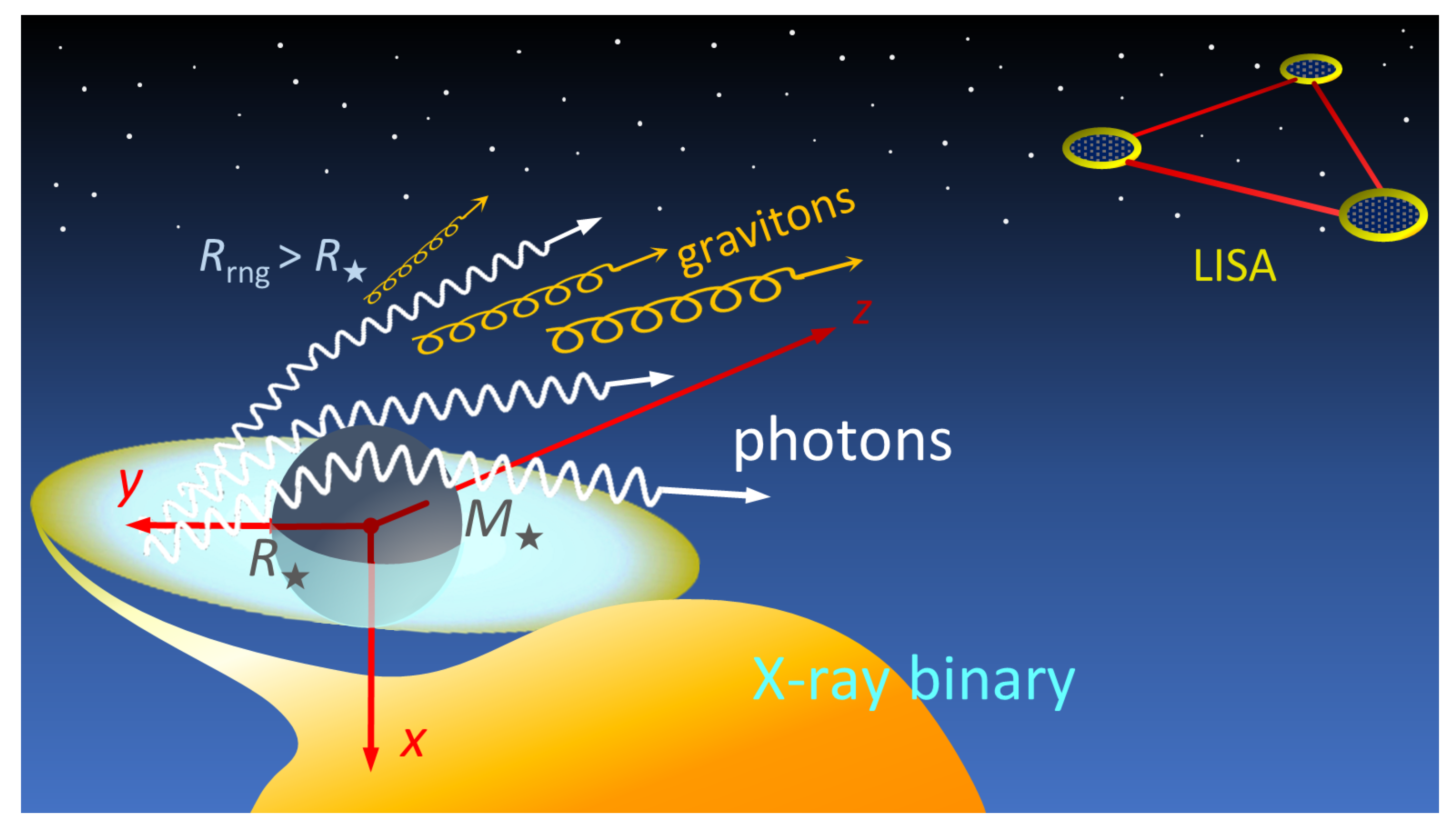
with and the gravitational constant G. Figure 1 illustrates the schematic physical and geometrical configurations under consideration.
Treating the above source as a gravitational lens, its effective refractive index is given approximately by [26]. This gives rise to the approximate dispersion relation
for a real massless scalar field having a frequency and wave vector p with wave number . We will continue to denote wave vectors associated with the scalar field by and and wave vectors associated with the gravitons by , unless otherwise stated.
To capture the salient physical effects carried by the light frequency and to simplify our technical derivations, we consider the wave number of the scalar to peak around some fixed value . Then, it follows from Equation (4) to leading contributions, that
where
Using Equation (6), the Lagrangian density of the scalar field
reduces to
with as the effective external scalar potential [27,28].
The stress–energy tensor of the scalar field is given by
The field equation follows as
To solve this field equation, one naturally invokes the separable ansatz
so that the general solutions are the real parts of the linear combinations of Equation (10). Substituting the above ansatz into Equation (9), we see that this field equation is equivalent to
taking the form of a time-independent Schrödinger equation.
It follows that the solutions to the field Equation (9) representing the deflection of light with an incident wave vector p and frequency can be obtained from the solutions of the Schrödinger Equation (11) describing a scattering problem involving a Coulomb-type, i.e., , central potential as the “scattering wave functions” of the form
where , , are spherical harmonics, and are the Coulomb wave functions satisfy the wave equation (see e.g., [29])
using the dimensionless variable and dimensionless parameter with
By virtue of the orthogonality of , we can choose the normalisation of so that satisfy the following orthonormality
It is useful to introduce the “momentum representation” scattering wave functions [30] of the above “position representation” scattering wave functions given by
For a weak interaction with the central potential where , the first order Born approximation yields
Note that the first term of Equation (21) corresponds to the first term of Equation (22), which represents the incident (asymptotically) free particle. This term does not contribute to Equation (31) under Markov approximation of the gravitational master equation as discussed in Reference [9].
The corresponding asymptotic scattering wave function of the position is given by
with the scattering amplitude
where is the scattering angle.
Just as with the Coulomb potential, so does the infinitely long range of the Newtonian potential imply a divergent total scattering cross section. However, to account for the realistic limited dominance of this potential due to other influences beyond a range distance , which can be conveniently incorporated by modifying the Newtonian potential with an additional exponential-decay factor of as a long-range regularisation. On the other hand, the finite extension with a radius of the gravity source means the need for a compensating short-range potential within this radius.
These considerations lead to the following phenomenological Yukawa regularisation
with and as long and short range regularisation parameters, respectively.
Accordingly, we find the regularised scattering wave function to be
with .
3. Quantisation of the Scalar Field in the Regularised Potential
Using scattering wave function derived in the preceding section, we can now perform the so-called second quantisation of the scalar field into a quantum field operator in the Heisenberg picture as follows
where ℏ is the reduced Planck constant and the creation and annihilation operators and satisfy the standard nontrivial canonical commutation relation
The associated field momentum is given by , which satisfies the equal time field commutation relation
following from Equations (16) and (27).
Substituting Equation (18) into Equation (26), we can write in terms of the momentum representations of the scattering wave functions as follows
The coupling of to the metric fluctuations due to low energy quantum gravity in addition to the metric perturbation Equation (2) due to the lensing mass is through the transverse-traceless (TT) part of its stress–energy tensor Equation (8) to be [8] given by
with the Fourier transform
where is the TT projection operator [8,31].
Using Equation (28) and applying normal orders and neglecting and terms through the rotating wave approximation [32], we see that Equation (30) becomes
From Equation (31) we see that
as a useful property for later derivations.
4. Coupling to the Gravitational Quantum Vacuum
To induce the spontaneous emission of the photon lensed by the regularised Newtonian potential, we now include an additional TT gravitational wave-like metric perturbation into Equation (1), which carries spacetime fluctuations at zero temperature [8]. The photon is assumed to travel a sufficiently long distance and time past the gravitational lens (see justifications below) so that we can neglect any memory effects in its statistical interactions with spacetime fluctuations. Additionally, we consider the energy scale to be low enough for the self interaction of the photon to be negligible. This leads to the Markov quantum master equation
in the interaction picture, where , is given by Equation (31), and H.c. denotes the Hermitian conjugate of a previous term, for the reduced density operator, i.e., density matrix, of the photon by averaging, i.e., tracing, out the degrees of freedom in the noisy gravitational environment [8,10].
We then apply the Sokhotski–Plemelj theorem
where is the Cauchy principal value. Since this Cauchy principal value contributes to a renormalised energy that can be absorbed in physical energies [32], we can neglect it.
Due to the weakness of interactions, the density matrix will evolve only slightly over time so that
where is the initial density matrix and the components of are small compared to the components of .
Then Equation (39) yields
For , physically corresponding to t greater than the effective interaction time of the system, we can again apply the Sokhotski–Plemelj theorem Equation (38) to Equation (41) and neglect the Cauchy principal value terms to obtain
More precisely, the limit , means t exceeds the effective interaction duration between the photon and the lensing mass with an effective force range , and this is satisfied if the photon is measured at a large distance with . Considering the time integrals in Equation (41), the validity of the foregoing limit is further justified through the numerical simulations described towards the end of this paper where k and are found to peak around .
Adopting the Born approximation (25) and keeping up to the first orders in , we see that Equation (35) becomes
in terms of
satisfying
which are consistent with Equation (32).
Substituting Equations (43) into Equation (42) and repetitively using the same argument leading to free particles suffering no Markovian gravitational decoherence, we obtain the 2nd order (in ) asymptotic change of the density matrix
On account of Equations (14) and (47), Equation (48) takes a more explicit form as follows
where
is a dimensionless parameter.
The action of Equation (49) can be obtained from its action on an initial basis matrix element of the form
Substituting this form (51) into Equation (49) and using the relation
obtained from Equation (27), we can usefully write the resulting as
where
does not lose energy and
is responsible for dissipating photon energy by emitting bremsstrahlung gravitons.
The setup above allows us to consider a wave packet profile
as an initial normalised state with
and a mean wave number vector so that
This can be used to construct an initial density matrix
5. Gravitational Bremsstrahlung with a Single Momentum Initial State
For simplicity, we now restrict to single momentum initial state, deferring the more general wave-packet initial states to a future investigation.
Such a state is obtained by setting in Equation (51) so that Equation (54) takes the form
where
with the dimensionless TT amplitude
There are two orthogonal parts of :
corresponding to the two (+ and ×) polarisations of the gravitational waves [31], so that the gravitational wave square amplitude decomposes accordingly as
For numerical evaluations, we can conveniently choose , then we have
For example, in the limit of a point source of gravity with effective radius , Equation (63) yields
where
and
It is also useful to introduce . For simplicity, let us adopt as a reasonable first order-of-magnitude estimate of the gravitational wave square amplitude for a source of gravity with an effective range and radius to be
To obtain an expression in term of dimensionless quantities, we express as dimensionless quantities in units of .
Then, by replacing and using Equation (50) with the mass–energy of the gravity source , we arrive at the fractional energy loss given by
where is the Planck energy and
with obtained from Equation (64) for and
We also have analogous constructions for and . Numerical evaluations of and as functions of show sharp but finite peaks around small k, and for small . This leads to finite numerical integrations with for . Therefore, for a gravity source with a characteristic radius and effective range in units of , from Equation (67) we have
approximately, corresponding to the rough spread of the photon impact parameter to be from the surface of the gravitational lens to one radius from the surface.
The energy loss rate above can be interpreted where is the effective graviton emission transition rate by the photon, and is the effective interaction time between the photon and the lensing mass with the corresponding effective interaction range . See Figure 1. This is consistent with the long travel time or distance assumption stated in Section 4.
6. Conclusions and Discussion
Based on the gravitational quantum vacuum, which has recently been shown to lead to gravitational decoherence [8] and gravitational spontaneous radiation that recovers the well-established quadrupole radiation [10], in this paper we have presented, to our knowledge, the first approach to the spontaneous bremsstrahlung of light due to the combined effects of gravitational lensing and spacetime fluctuations. Our present work yields a new quantum gravitational mechanism whereby starlight emits soft gravitons and becomes partially redshifted. This effect may contribute to the stochastic gravitational wave background [11,33,34]. We also note that while the term (53) for the outgoing light does not undergo photon to graviton energy conversion, it exhibits a type of recoherence of photons [35].
Our work naturally raises the prospect of potential detection of the released stochastic gravitational waves. Addressing this question in detail requires a further investigation, which is currently underway by the authors. It is however of interest at the present stage to envisage a plausible observation scenario. To this end, let us take the well studied strong X-ray binary Cygnus X-1 [36] because this system has both a large gravitational field and a strong X-ray source similar to that illustrated in Figure 1. However, both the compact object/black hole and the companion supergiant star in the Cygnus X-1 binary system are massive, with a total mass and an orbiting radius , which we will take as the effective . This would make to be in the region of and so from the discussions in Section 5, the spontaneously emitted stochastic gravitational waves would have a mean wavelength in the same region having a mean frequency Hz. Using these parameters, the fractional energy loss in Equation (71) is plotted in Figure 2 with the effective gravity range parameter chosen to be , corresponding to the rough spread of the photon impact parameter to be from the surface of the gravitational lens to discussed above. The detection of sub-Hz gravitational waves is a unique strength of the proposed LISA mission, which is expected to reach a corresponding characteristic strain sensitivity close to [37], as shown in Figure 3.
From the X-ray luminosity of Cygnus X-1 erg s [38,39] and its distance light years to the Earth, one gets the arriving X-ray energy flux to be erg cms. Let us suppose that the total gravitational wave luminosity of Cygnus X-1 arises from , in terms of an effective photon-to-graviton energy transfer rate . We can then estimate the characteristic strain h of the gravitational waves with energy density expression where with and the energy flux so that . For example, if and Hz, then erg cms yielding .
As shown in Figure 3, we choose moderate effective transfer rate values across the gravitational wave frequencies Hz 10 Hz. Indeed, for at around 0.01 Hz, the characteristic strain of the bremsstrahlung gravitational waves from Cygnus X-1 could be above the sensitivity level of LISA and hence potentially detectable. Furthermore, the buildup of similar sources could also contribute to an overall stochastic gravitational wave background. Based on the initial results and estimates reported in this work, we plan to analyse and quantify the properties of the bremsstrahlung gravitational waves from intense astronomical sources of light and gravity in a more realistic setting for future publication.
Author Contributions
Conceptualisation, C.H.-T.W.; methodology, C.H.-T.W. and M.M.; software, C.H.-T.W. and M.M.; validation, C.H.-T.W. and M.M.; formal analysis, C.H.-T.W.; investigation, C.H.-T.W.; resources, C.H.-T.W. and M.M.; data curation, C.H.-T.W. and M.M.; writing—original draft preparation, C.H.-T.W.; writing—review and editing, C.H.-T.W. and M.M.; visualisation, C.H.-T.W. and M.M.; supervision, C.H.-T.W.; project administration, C.H.-T.W.; funding acquisition, C.H.-T.W. and M.M. Both authors have read and agreed to the published version of the manuscript.
Funding
C.W. was funded by the Cruickshank Trust and M.M. was funded by the Student Awards Agency Scotland (SAAS).
Institutional Review Board Statement
Not applicable.
Informed Consent Statement
Not applicable.
Data Availability Statement
Acknowledgments
C.W. wishes to thank John S. Reid for many years of stimulating discussions on the topics and background of this work.
Conflicts of Interest
The authors declare no conflict of interest.
References
- Jaynes, E.T.; Cummings, F.W. Comparison of quantum and semiclassical radiation theories with application to the beam maser. Proc. IEEE 1963, 51, 89–109. [Google Scholar] [CrossRef] [Green Version]
- Gregori, G.; Bingham, R.; Eneh, B.; Wang, C.H.-T. How Can We Probe the Quantum Nature of Black Holes with High Power Lasers? 2021; In preparation. [Google Scholar]
- Crowley, B.J.B.; Bingham, R.; Evans, R.G.; Gericke, D.O.; Landen, O.L.; Murphy, C.D.; Gregori, G. Testing quantum mechanics in non-Minkowski space-time with high power lasers and 4th generation light sources. Sci. Rep. 2012, 2, 491. [Google Scholar] [CrossRef] [PubMed]
- Wang, C.H.-T.; Stankiewicz, M. Quantization of time and the big bang via scale-invariant loop gravity. Phys. Lett. B 2020, 800, 135106. [Google Scholar] [CrossRef]
- Wang, C.H.-T.; Rodrigues, D.P.F. Closing the gaps in quantum space and time: Conformally augmented gauge structure of gravitation. Phys. Rev. D 2018, 98, 124041. [Google Scholar] [CrossRef] [Green Version]
- Veraguth, O.J.; Wang, C.H.-T. Immirzi parameter without Immirzi ambiguity: Conformal loop quantization of scalar-tensor gravity. Phys. Rev. D 2017, 96, 044011. [Google Scholar] [CrossRef] [Green Version]
- Burgess, C.P. Quantum gravity in everyday life: General relativity as an effective field theory. Living Rev. Relativ. 2004, 7, 5. [Google Scholar] [CrossRef] [Green Version]
- Oniga, T.; Wang, C.H.-T. Quantum gravitational decoherence of light and matter. Phys. Rev. D 2016, 93, 044027. [Google Scholar] [CrossRef] [Green Version]
- Oniga, T.; Wang, C.H.-T. Spacetime foam induced collective bundling of intense fields. Phys. Rev. D 2016, 94, 061501(R). [Google Scholar] [CrossRef] [Green Version]
- Oniga, T.; Wang, C.H.-T. Quantum coherence, radiance, and resistance of gravitational systems. Phys. Rev. D 2017, 96, 084014. [Google Scholar] [CrossRef] [Green Version]
- Quiñones, D.A.; Oniga, T.; Varcoe, B.T.H.; Wang, C.H.-T. Quantum principle of sensing gravitational waves: From the zero-point fluctuations to the cosmological stochastic background of spacetime. Phys. Rev. D 2017, 96, 044018. [Google Scholar] [CrossRef] [Green Version]
- Misner, C.W.; Thorne, K.S.; Wheeler, J.A. Gravitation; Freeman: New York, NY, USA, 1973. [Google Scholar]
- Oniga, T.; Wang, C.H.-T. Quantum dynamics of bound states under spacetime fluctuations. J. Phys. Conf. Ser. 2017, 845, 012020. [Google Scholar] [CrossRef]
- Baker, R.M., Jr.; Baker, B.S. Gravitational wave generator apparatus. Phys. Procedia 2012, 38, 288. [Google Scholar] [CrossRef] [Green Version]
- Raffelt, G.G. Particle physics from stars. Annu. Rev. Nucl. Part. Sci. 1999, 49, 163–216. [Google Scholar] [CrossRef] [Green Version]
- Papini, G.; Valluri, S.-R. Photoproduction of high-frequency gravitational radiation by galactic and extragalactic sources. Astron. Astrophys. 1989, 208, 345. [Google Scholar]
- Del Campo, S.; Ford, L.H. Graviton emission by a thermal bath of photons. Phys. Rev. D 1988, 38, 3657. [Google Scholar] [CrossRef] [PubMed]
- Gould, R.J. The graviton luminosity of the sun and other stars. Astrophys. J. 1985, 288, 789. [Google Scholar]
- Ford, L.H. Gravitational radiation by quantum systems. Ann. Rev. 1982, 144, 238. [Google Scholar]
- Grishchuk, L.P. Gravitational waves in the cosmos and the laboratory. Sov. Phys. Usp. 1977, 20, 319. [Google Scholar] [CrossRef]
- Grishchuk, L.P. Emission of gravitational waves by an electromagnetic cavity. Zh. Eksp. Teor. Fiz. 1973, 65, 441. [Google Scholar]
- Lebed’, A.A.; Roshchupkin, S.P. Resonant spontaneous bremsstrahlung by an electron scattered by a nucleus in the field of a pulsed light wave. Phys. Rev. A 2010, 81, 033413. [Google Scholar] [CrossRef]
- Breuer, H.-P.; Petruccione, F. Destruction of quantum coherence through emission of bremsstrahlung. Phys. Rev. A 2001, 63, 032102. [Google Scholar] [CrossRef]
- Karapetyan, R.V.; Fedorov, M.V. Spontaneous bremsstrahlung of an electron in the field of an intense electromagnetic wave. J. Exp. Theor. Phys. 1978, 48, 412. [Google Scholar]
- Bethe, H.; Heitler, W. On the stopping of fast particles and on the creation of positive electrons. Proc. Roy. Soc. A 1934, 146, 83. [Google Scholar]
- Meylan, G.; Jetzer, P.; North, P. (Eds.) Gravitational Lensing: Strong, Weak and Micro; Springer: Berlin, Germany, 2006. [Google Scholar]
- Milton, K.A. Hard and soft walls. Phys. Rev. D 2011, 84, 065028. [Google Scholar] [CrossRef] [Green Version]
- Milton, K.A.; Fulling, S.A.; Parashar, P.; Kalauni, P.; Murphy, T. Stress tensor for a scalar field in a spatially varying background potential. Phys. Rev. D 2016, 93, 085017. [Google Scholar] [CrossRef] [Green Version]
- Wong, S.S.M. Introductory Nuclear Physics; WILEY-VCH: Weinheim, Germany, 2004. [Google Scholar]
- Guth, E.; Mullin, C.J. Momentum representation of the Coulomb scattering wave functions. Phys. Rev. 1951, 83, 667. [Google Scholar]
- Flanagan, E.E.; Hughes, S.A. The basics of gravitational wave theory. New J. Phys. 2005, 7, 204. [Google Scholar] [CrossRef]
- Breuer, H.-P.; Petruccione, F. The Theory of Open Quantum Systems; Oxford University Press: New York, NY, USA, 2002. [Google Scholar]
- Christensen, N. Stochastic gravitational wave backgrounds. Rep. Prog. Phys. 2019, 82, 016903. [Google Scholar]
- Allen, B. The stochastic gravity-wave background. arXiv 1996, arXiv:gr-qc/9604033. [Google Scholar]
- Bouchard, F.; Harris, J.; Mand, H.; Bent, N.; Santamato, E.; Boyd, R.W.; Karimi, E. Observation of quantum recoherence of photons by spatial propagation. Sci. Rep. 2015, 5, 15330. [Google Scholar] [CrossRef] [Green Version]
- Bel, M.C.; Sizun, P.; Goldwurm, A.; Rodriguez, J.; Laurent, P.; Zdziarski, A.A.; Roques, J.P. The broad-band spectrum of Cygnus X-1 measured by INTEGRAL. Astron. Astrophys. 2006, 446, 591–602. [Google Scholar]
- Moore, C.J.; Cole, R.H.; Berry, C.P.L. Gravitational-wave sensitivity curves. Class. Quantum Grav. 2015, 32, 015014. [Google Scholar] [CrossRef]
- Liang, E.P.; Lolan, P.L. CYGNUS-X-1 Revisited. Space Sci. Rev. 1984, 38, 353. [Google Scholar] [CrossRef]
- Wen, L.; Cui, W.; Levine, A.M.; Bradt, H.V. Orbital modulation of x-rays from Cygnus X-1 in its hard and soft states. Astrophys. J. 1999, 525, 968. [Google Scholar] [CrossRef]
Figure 1.
An illustration of the key physical and geometrical features of an astronomical configuration for the gravitational bremsstrahlung of light involving an X-ray binary and a possible detection concept with LISA. Here the mass of the compact object is assumed to be dominant for simplicity.
Figure 1.
An illustration of the key physical and geometrical features of an astronomical configuration for the gravitational bremsstrahlung of light involving an X-ray binary and a possible detection concept with LISA. Here the mass of the compact object is assumed to be dominant for simplicity.

Figure 2.
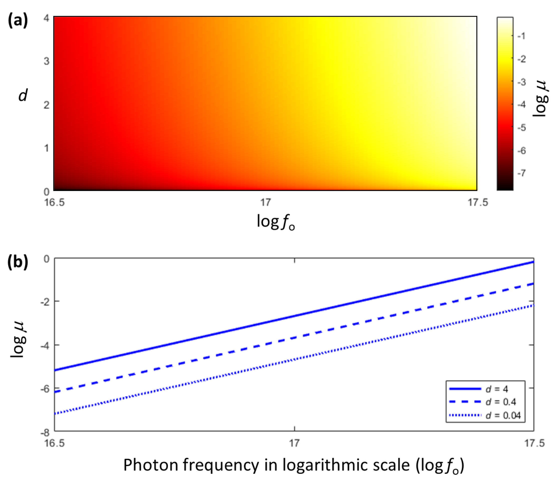
The fractional energy loss given by Equation (71) as a function of the photon frequency (Hz) in logarithmic scale along the horizontal axis evaluated with a chosen range of the effective gravity range parameter for the X-ray binary Cygnus X-1. Above, is plotted in (a) as a projected height onto the plane and in (b) as a line for three representative values of d. It is obvious that as the photon frequency increases from the optical spectrum, the photon-to-graviton energy conversion “chips in” at around Hz at the start of the soft X-ray spectrum, so that for corresponding to . Although here appears to carry on increasing with , the validity of Equation (71) is strictly limited to small due to the Born approximation with weak interactions we have assumed in Equation (21) used to derive in Equation (71). Nonetheless, the ascending trend of with the photon frequency suggests that starting from the soft X-ray frequencies, the gravitational bremsstrahlung of light in the vicinity of Cygnus X-1 may be important.
Figure 2.
The fractional energy loss given by Equation (71) as a function of the photon frequency (Hz) in logarithmic scale along the horizontal axis evaluated with a chosen range of the effective gravity range parameter for the X-ray binary Cygnus X-1. Above, is plotted in (a) as a projected height onto the plane and in (b) as a line for three representative values of d. It is obvious that as the photon frequency increases from the optical spectrum, the photon-to-graviton energy conversion “chips in” at around Hz at the start of the soft X-ray spectrum, so that for corresponding to . Although here appears to carry on increasing with , the validity of Equation (71) is strictly limited to small due to the Born approximation with weak interactions we have assumed in Equation (21) used to derive in Equation (71). Nonetheless, the ascending trend of with the photon frequency suggests that starting from the soft X-ray frequencies, the gravitational bremsstrahlung of light in the vicinity of Cygnus X-1 may be important.

Figure 3.
Estimated characteristic strain h of the gravitational waves with effective photon-to-graviton energy transfer rate for Cygnus X-1 with against the gravitational wave frequency f in Hz compared with the LISA characteristic strain sensitivity curve [37].
Figure 3.
Estimated characteristic strain h of the gravitational waves with effective photon-to-graviton energy transfer rate for Cygnus X-1 with against the gravitational wave frequency f in Hz compared with the LISA characteristic strain sensitivity curve [37].

Publisher’s Note: MDPI stays neutral with regard to jurisdictional claims in published maps and institutional affiliations. |
© 2021 by the authors. Licensee MDPI, Basel, Switzerland. This article is an open access article distributed under the terms and conditions of the Creative Commons Attribution (CC BY) license (https://creativecommons.org/licenses/by/4.0/).
Share and Cite
MDPI and ACS Style
Wang, C.H.-T.; Mieczkowska, M. Bremsstrahlung of Light through Spontaneous Emission of Gravitational Waves. Symmetry 2021, 13, 852. https://doi.org/10.3390/sym13050852
AMA Style
Wang CH-T, Mieczkowska M. Bremsstrahlung of Light through Spontaneous Emission of Gravitational Waves. Symmetry. 2021; 13(5):852. https://doi.org/10.3390/sym13050852
Chicago/Turabian StyleWang, Charles H.-T., and Melania Mieczkowska. 2021. "Bremsstrahlung of Light through Spontaneous Emission of Gravitational Waves" Symmetry 13, no. 5: 852. https://doi.org/10.3390/sym13050852
Note that from the first issue of 2016, this journal uses article numbers instead of page numbers. See further details here.