Machine and Deep Learning Applied to Predict Metabolic Syndrome without a Blood Screening

Abstract

The exponential increase of metabolic syndrome and its association with the risk impact of morbidity and mortality has propitiated the development of tools to diagnose this syndrome early. This work presents a model that is based on prognostic variables to classify Mexicans with metabolic syndrome without blood screening applying machine and deep learning. The data that were used in this study contain health parameters related to anthropometric measurements, dietary information, smoking habit, alcohol consumption, quality of sleep, and physical activity from 2289 participants of the Mexico City Tlalpan 2020 cohort. We use accuracy, balanced accuracy, positive predictive value, and negative predictive value criteria to evaluate the performance and validate different models. The models were separated by gender due to the shared features and different habits. Finally, the highest performance model in women found that the most relevant features were: waist circumference, age, body mass index, waist to height ratio, height, sleepy manner that is associated with snoring, dietary habits related with coffee, cola soda, whole milk, and Oaxaca cheese and diastolic and systolic blood pressure. Men’s features were similar to women’s; the variations were in dietary habits, especially in relation to coffee, cola soda, flavored sweetened water, and corn tortilla consumption. The positive predictive value obtained was 84.7% for women and 92.29% for men. With these models, we offer a tool that supports Mexicans to prevent metabolic syndrome by gender; it also lays the foundation for monitoring the patient and recommending change habits.

1. Introduction

Nowadays, chronic degenerative diseases, such as ischemic heart disease, type 2 diabetes mellitus, and cerebrovascular stroke, are the leading causes of morbidity and mortality worldwide; these diseases share one or more metabolic components (glucose intolerance, insulin resistance, central obesity, dyslipidemia, and hypertension) that might co-exist in one individual. The term Metabolic Syndrome (MetS) was coined to express this constellation of metabolic abnormalities [1].

The prevalence of MetS in Mexico is 41% [2] higher than in developed countries, like the United States (34.2%) [3], due to the epidemic proportion that overweight and obesity have taken in our country, affecting not only the adult population, but also young individuals and even children, with obesity being a central, key component of MetS.

The evaluation criteria for MetS have been proposed by the National Cholesterol Education Program Adult Treatment Panel III (NCEP ATP III) [4], the International Diabetes Federation (IDF) [5,6], and the World Health Organization (WHO) [7]. In order to establish a clinical diagnose of MetS, at least three metabolic abnormalities mostly co-occurr in the same individual: elevated blood sugar levels, insulin resistance, abdominal obesity, high blood pressure, and abnormal lipid profile (high blood levels of triglyceride and low blood levels of high-density lipoprotein cholesterol).

These evaluation criteria have been useful from a clinical point of view. However, from the general population perspective, its utility is limited, since laboratory screening is needed [8], which can be costly or cumbersome to implement for certain population levels. The above and the fact that most people are unaware of their health condition, and approach health services until the sickness has caused health limitations [9,10,11]. For this reason, it is essential to generate tools that can help people to identify pre-clinical conditions, so that preventive measures can be taken at a population level.

The application of machine learning and deep learning (DL) algorithms has facilitated the construction of effective models to predict disease diagnoses and the corresponding treatments [12,13]. However, the appropriate selection of variables (potential risk factors) is decisive in improving the models [14,15,16].

In the case of MetS, the use of machine learning and deep learning algorithms, as well as feature selection methods, have achieved significant results in the development of models to support the prediction of this syndrome [17,18]. Related studies that have omitted blood screening for the diagnosis of the MetS have had promising results. An investigation conducted by Barrios et al. [19], proposed a data mining methodology to diagnose MetS without blood screening by applying Artificial Neural Networks (ANN).

In that work, hip circumference, dichotomous waist circumference, dichotomous blood pressure, and sex were included; the specificity reported was 82.59%, a Positive Predictive Value (PPV) of 90.54%, and an Area under the Receiver Operating Characteristic (ROC) Curve of 87.36%. Romero et al. [20] constructed a model applying ANN and considering variables, such as Body Mass Index (BMI), Waist Circumference (WC), weight, height, and sex. The authors used PPV as an evaluation metric, obtaining a value of 38.8%.

Ivanović et al. [21] presented a model using ANN for the prediction of MetS, excluding blood screening. The features that result in this study were: gender, age, BMI, Waist-to-height Ratio (WhtR), systolic, and diastolic blood pressures, with a PPV of 85.79% and Negative Predictive Value (NPV) of 83.19%.

Another study relates the dietary habits with MetS in the Swedish region. The authors used chi-square analysis [22]. They found four patterns that were defined by clusters that demonstrated a strong association between food and components of MetS. For example, hyperglycemia in men was associated with cheese, cake, and alcoholic beverages consumption; a higher risk of hyperinsulinemia and dyslipidemia in women was associated with white bread consumption. That work was relevant, since different patterns were used for each gender.

The purpose of this article is to identify the most relevant features to propose a risk predictor for the early detection of people with MetS, through machine learning algorithms, such as Random Forest (RF), Ripper (C4.5), and deep neural networks, when considering traditional risk factors for this syndrome as well as dietary information [23,24] and habits, like the consumption of alcoholic beverages [25], smoking [26], physical activity [27], and quality of sleep [28].

This paper is structured, as follows: in Section 2, we introduce the materials and methods. In Section 3, we present the experiments performed and the results. Section 4 shows the discussion, and, finally, the conclusions.

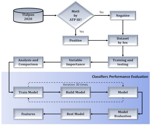
2. Materials and Methods

2.1. Data

The data set used in this research was collected from the Tlalpan 2020 cohort, a study that was conducted by the Instituto Nacional de Cardiología Ignacio Chávez in Mexico City [29]. The Tlalpan 2020 cohort was approved by the Institutional Bioethics Committee of the Instituto Nacional de Cardiología-Ignacio Chavez (INC-ICh) under code 13-802. This work consists of 2289 subjects between 20 and 50 years old, 1369 women, and 920 men, it is important to mention that informed consent was obtained from all the participants. The prevalence of MetS, according to NCEP ATP III criteria, was 24.4% higher in women (54%) than in men (46%). This data set includes health parameters and habits that are related to alcohol consumption, smoking, physical activity, dietary, and quality of sleep.

2.1.1. Clinical and Anthropometric Parameters

Systolic and diastolic blood pressure were measured according to The Seventh Report of the Joint National Committee on the Prevention, Detection, Evaluation, and Treatment of High Blood Pressure (JNC 7) standard procedure [30]. WC, height, and weight were measured according to The International Society for the Advancement of Kinanthropometry (ISAK) [31], BMI was calculated as weight/height${}^2$ and WHtR was calculated as the ratio of waist and height (wast/height) (cm).

2.1.2. Biochemical Evaluation

The blood samples were taken after 12 h of overnight fasting, and the following laboratory tests measurements were obtained: fasting plasma glucose (FPG), triglycerides (TGs), and HDL cholesterol (HDL-C) cholesterol LDL (LDL-C), total cholesterol (T-C).

2.1.3. Dietary Information

Dietary information was collected using the nutrient software program known as Sistema de Evaluación de Hábitos Nutricionales y Consumo de Nutrimientos (SNUT) (Evaluation of Nutritional Habits and Nutrient Consumption System) [32], as developed by the Instituto Nacional de Salud Pública de México (National Institute of Public Health of Mexico). The SNUT includes data from various types of nutrients classified into different categories, such as dairy products, fruits, meats, vegetables, legumes, cereals, sweets and candies, beverages, fats, cravings, and others. All of the variables of the SNUT were included, and their nominal numerical value was considered, which is, the frequency of food consumption during the day, in the last year.

2.1.4. Habits

The following lifestyle information was collected; furthermore, they are inputs for the machine and deep learning algorithms: (1) the smoking habit that was summed up as never smoked, former, or current smoker, and the three features are dichotomous. (2) Alcohol consumption that was classified as a current drinker (dichotomous variable), frequency alcohol consumption, and cups or beers consumed on average when drinking alcohol; these last two are considered to be numeric variables according to the weekly ingesting. (3) Physical activity was obtained by the extended version of the International Physical Activity Questionnaire, IPAQ, [33] that measures the level of physical activity as low, moderate, and high, through questions regarding four domains: work, home, transportation, and leisure time; for this paper, we used the nominal numerical value of variables that are related with leisure time domain, like the days and duration of the type of physical activity (walking, moderate, or vigorous) per week in the last seven days. Lastly (4), quality of sleep was obtained employing the Medical Outcomes Study-Sleep Scale (MOSS) [34], we consider the nominal numerical value of these variables, where the values are described in [35].

2.2. Methods

For the study, we applied three machine learning algorithms, RF, C4.5, and deep learning. We conducted experiments for each sex. We choose these machine learning algorithms because of their excellent results in many applications and because each one uses a different approach in a classification task [18,19,36]. We also performed feature selection to search for simpler and better models. The experiments were conducted using R programming language [37]. We aimed to predict the MetS without using biochemical variables.

Initially, the parameters of the biochemical evaluation, as well as the anthropometric factors: waist circumference, systolic and diastolic blood pressure, glucose, high-density lipoprotein cholesterol (HDL), and triglycerides, in order to identify and classify participants with MetS based on the definition that was established by the NCEP ATP III. Once the participants have been classified as positive and negative concerning the MetS, the input dataset for the learning algorithms is generated, being composed of categories related to clinical and anthropometric parameters and habits, like alcohol consumption, smoking, physical activity, dietary, and quality of sleep.

The performance of the models was evaluated according to accuracy, balanced accuracy, PPV, and NPV. Figure 1 shows a block diagram of the prediction model and describes the general methodology applied. As a first step, the instances of the data set were classified using the biochemical evaluation data and the clinical and anthropometric parameters, according to the NCEP ATP III criteria. Subsequently, we separated men and women to obtain the most important variables for each sex.

We applied RF to identify and evaluate the variable importance by category, as well as Pearson Correlation Coefficient (PCC) and chi-square, to obtain the most important variables when considering all of the categories together.

We created and evaluated predictive models using the ML algorithms for different subgroups that formed based on the variables obtained. From these models, we selected the most relevant features for men and women.

In all experiments, we performed 30 independent runs by algorithm, which is a typical number that is used in the literature for fair comparisons among experiments [38,39]. Subsequently, we calculated the mean and standard deviation for each metric.

2.2.1. Random Forest

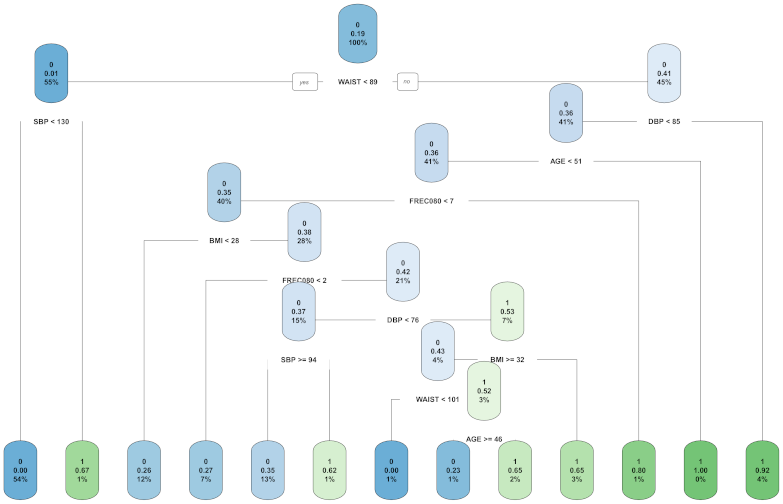
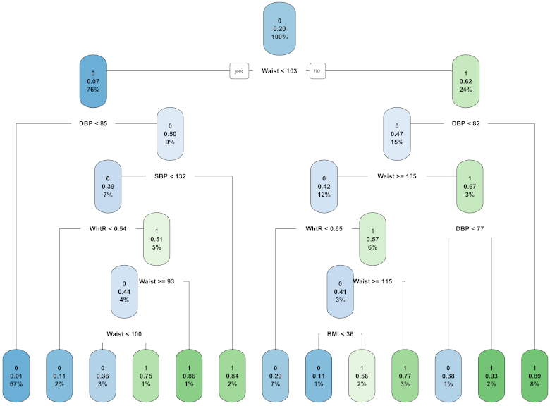
RF, as introduced by Breiman [40], is a machine learning algorithm that is based on a combination of tree estimators that operate as an ensemble for classification and regression cases. In this work, this method was used for the classification and identification of the importance of the variables, based on the mean decrease impurity [41], which is a method that is measured by the Gini index for variable $x_j$, and it is computed by the equation:

$$VI=\left(X_j\right)=\frac{1}{n_{tree}}\left[1-\sum _{k=1}^{ntree}Gini{\left(j\right)}^k\right]$$

(1)

where ntree is the number of trees.

2.2.2. C4.5

C4.5 builds a decision tree from training data using recursive partitions. In each iteration, C4.5 selects the attribute with the highest gain ratio as the attribute from which the tree is branched. This results in a more simplified tree [42,43]. In order to obtain the gain ratio, the following calculations are needed:

$$EntropyH\left(S\right)=-\sum _{i=1}^m{p}_{i}lo{g}_2{p}_i$$

(2)

where S is a set consisting of s data samples with m distinct classes, and $p_i$ is the probability that an arbitrary sample belongs to class $C_i$.

Let attribute A have v distinct values. The entropy, or expected information based on the partitioning into subsets by A, is given by:

$$InformationGainI(S,A)=H\left(S\right)-H\left(S\right|A)$$

(3)

$$SplitInf{o}_A\left(S\right)=\sum _{i=1}^v(\left|S_i\right|/\left|S\right|)lo{g}_2(\left|S_i\right|/\left|S\right|)$$

(4)

$SplitInfo$ represents the information that is generated by splitting the training data set S into v partitions, corresponding to v outcomes of a test on the attribute A.

Finally, the gain ratio is defined, as follows:

$$GainRatio=InformationGain/SplitInfo$$

(5)

2.2.3. Chi-Squared

Chi-Squared is a statistical test that is used in machine learning to identify the essential features in a dataset for a classification task [44]. It gives a feature ranking as a result. Taking a feature f and the class c ($\overline{f}$, $\overline{c}$ as complements), the chi-squared test is computed with the equation:

$$X^2(f,c)=\frac{N{[P(f,c)P(\overline{f},\overline{c})-P(f,\overline{c})P(\overline{f},c)]}^2}{P\left(f\right)P\left(\overline{f}\right)P\left(c\right)P\left(\overline{c}\right)}$$

(6)

where N is the number of records in the dataset. $P(x,y)$ is the joint probability of x and y. $P\left(x\right)$ is the marginal probability of x.

2.2.4. Pearson Correlation

For the statistical analysis, the PCC was used to filter features [45]. Those with a correlation coefficient above 0.5 were used to train machine or deep learning algorithms. This relation is defined by Equation (7) [46]:

$$pcc(u,u^{\prime })=\frac{{\sum }_{i\in I}(r_{u,i}-{\overline{r}}_u)(r_{u^{\prime },i}-{\overline{r}}_{u^{\prime }})}{\sqrt{{\sum }_{i\in I}{(r_{u,i}-{\overline{r}}_u)}^2}\sqrt{{\sum }_{i\in I}{(r_{u,i}-{\overline{r}}_{u^{\prime }})}^2}},$$

(7)

where $r_{u,i}$ and $r_{u^{\prime },i}$ are the rating scores, also ${\overline{r}}_u$ and ${\overline{r}}_{u^{\prime }}$ are the average ratings. In this work, we used PCC to find the highest correlation between the health parameters and, thus, select the most relevant features, as we mentioned before, with a threshold of 0.5. Additionally, it is essential to highlight and the output corresponds to the classification in the dataset labeled by NCEP ATP III criteria. With this procedure, we aimed at improving the performance of the predictive models.

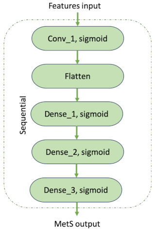
2.2.5. Deep Neural Networks

The basis for the development of deep learning is ANN, that through the connection among many hidden layers, can learn features to train the model [47]. In this work, Keras was used [48]; this model is based on a sequential class; it means that the network is created layer by layer. Only the dimension for the first layer corresponds to the number of features; then, the hidden layers’ dimension is deeply connected to the neural network. The first layer consists of a convolution network with an input shape of seven (features selected); after the first layer’s output is flattened, the purpose is to only have one dimension in the shape output. The third layer is a dense network with a dimension of 8, another dense network (dimension = 8) is added; finally, the last layer is a dense network; all of them have a sigmoid function for activation. Figure 2 shows the general configuration for the deep neural network implemented. The training parameters were a learning rate of 0.0001 and 2500 epochs with Adam optimization. The parameters were selected according to proof of good performance.

2.3. Metrics

For the evaluation of the model performance, we used the PPV, NPV, accuracy (ACC), and balanced accuracy (B.ACC).

$$PPV=\frac{TP}{TP+FP}$$

(8)

$$NPV=\frac{TN}{FP+FN}$$

(9)

$$ACC=\frac{TP+TN}{P+N}$$

(10)

$$B.ACC=\left(\frac{1}{2}\right)\left(\frac{TP}{P}+\frac{TN}{N}\right)$$

(11)

where P = Positive, N = Negative, TP = True Positive, FN = False Negative, TN = True Negative, and FP = False Positive, respectively.

3. Results

3.1. Variable Importance by Category

The first step was to separate the men and women data, then the essential variables by gender and category were obtained:

• clinical and anthropometric parameters,
• dietary information,
• quality of sleep, and
• habits (smoking, alcohol consumption, physical activity).

Applying the variable importance measures (VIM) of RF.

Table 1. (A) Most important variables in women by category. (B) Most important variables in women in whole dataset.

Category	Method	Resulting Variables
(A)
Feeding habits	VIM of RF	cola_soda, flav_soda, oax_cheese, c_coffe and flav_water
Quality of sleep	VIM of RF	snore, restless, lit_sleep, restless and drowsy
Anthropometry	VIM of RF	Waist, WHtR, BMI, SBP, DBP, and Age
Habits	VIM of RF	EtOH_AVG, smk.smke and exrcs
(B)
Whole Dataset	VIM of RF	Age, Waist, BMI, WHtR, Weight, Height, SBP, DBP, cola_soda, snore, oax_cheese and c_coffe
	PCC	Age, Weight, BMI, Waist, WHtR, SBP, DBP, snore, cola_soda and pork_r
	Chi.square	Age, BMI, Waist, WHtR, Weight, SBP, DBP, snore and cola_soda

(A) cola_soda: medium cola soda, flav_soda: soda, oax_cheese: Oaxaca cheese, c_coffe: cup of coffee, flav_water: flavor water, snore: snore during sleep, restless: restless sleep, lit_sleep: sleeps little, nt_sleep: not getting enough sleep, drowsy: feeling drowsy, EtOH_AVG: cups or beers consumed on average when drinking alcohol, smk.smke: smoke, exrcs: free physical activity. BMI: Body Mass Index, WHtR: Waist-to-Height-Ratio, SBP: systolic blood pressure, DBP: diastolic blood pressure. (B) cola_soda: medium cola soda, oax_cheese: Oaxaca cheese, c_coffe: cup of coffee, pork_r: pork rind, snore: snore during sleep, BMI: Body Mass Index, WHtR: Waist-to-Height-Ratio, SBP: systolic blood pressure, DBP: diastolic blood pressure.

A and

Table 2. (A) Most important variables in men by category. (B) Most important variables in men in whole dataset.

Cathegory	Method	Resulting Variables
(A)
Feeding habits	VIM of RF	cola_soda, flav_water, hot_chili, c_coffe and tortilla
Quality of sleep	VIM of RF	snore, nt_sleep, SLP SMN, restless and tired
Anthropometry	VIM of RF	DBP, Waist, SBP, WHtR, BMI and Age
Habits	VIM of RF	smk.smke, EtOH_AVG and exrcs
(B)
Whole Dataset	VIM of RF	DBP, Waist, BMI, WHtR, SBP, Weight, Age, snore, cola_soda, flav_water, c_coffe and tortilla
	PCC	Age, Weight, BMI, Waist, WHtR, SBP, DBP, snore and cola_soda
	Chi.square	BMI, Waist, DBP, SBP, Weight, WHtR, Age, snore and cola_soda

(A) cola_soda: medium cola soda, flav_water: a glass of flavored sweetened water, hot_chilli: a tablespoon of hot sauce or chili in food, c_coffe: a cup of coffee, tortilla: corn tortilla, snore: snore during sleep, nt_sleep: not getting enough sleep, drowsy: feeling drowsy, restless: restless sleep, tired: feel fatigue, smk.smke: smoke, EtOH_AVG: cups or beers consumed on average when drinking alcohol, exrcs: free physical activity, DBP: diastolic blood pressure, Waist: waist circumference, BMI: Body Mass Index, WHtR: Waist-to-Height-Ratio, SBP: systolic blood pressure. (B) cola_soda: medium cola soda, c_coffe: a cup of coffee, tortilla: corn tortilla, flav_water: a glass of flavored sweetened water, snore: snore during sleep, DBP: diastolic blood pressure, Waist: waist circumference, BMI: Body Mass Index, WHtR: Waist-to-Height-Ratio, SBP: systolic blood pressure.

A show the most important variables (in descending order) obtained for women and men, respectively.

3.2. Variable Importance of the Complete Dataset

As second step, the most important variables for women and men were obtained when considering the whole dataset. For this process, VIM of RF, chi.square, and PCC were applied, the resulting variables were compared with those that were obtained for each category to identify which ones were repeated in each case.

Table 1B and Table 2B show the most important variables (in descending order) for women and men while considering the whole dataset.

3.3. Most Important Variables in Women

We found that the five most important variables for women in the feeding habits category were: medium cola soda (cola_soda), soda (flav_soda), Oaxaca cheese (oax_cheese), a cup of coffee (c_coffe), and flavored water (flav_water). In the quality of sleep, the five most important variables were: snoring during sleep (snore), restless sleep (restless), little naps (lit_sleep), not getting enough sleep (nt_sleep), and feeling drowsy (drowsy). The five most important variables for the clinical and anthropometric parameters were: WC, DBP, WHtR, BMI, and SBP. In the category of habits, the most important variable was the cups or beers consumed on average when drinking alcohol (EtOH.avg), followed by smoke (smk.smke), and, finally, the free physical activity (exrcs). Table 1A presents these results.

Now, when considering the whole dataset, we applied VIM of RF, PCC, and chi.square to obtain the most important variables (see Table 1B). In the case of VIM of RF, it identified twelve variables, which were: age, waist, BMI, WHtR, weight, height, SBP, DBP, cola_soda, snore, oax_cheese, and c_coffe. Moreover, the PCC method determined ten variables, which were: age, weight, BMI, waist, WHtR, SBP, DBP, snore, cola_soda, and pork rind (pork_r). Finally, chi.square obtained nine variables: age, BMI, waist, WHtR, weight, SBP, DBP, snore, and cola_soda. Table 1B presents these results.

3.4. Most Important Variables in Men

In relation to feeding habits, the five most important variables were: cola_soda, flav_water, hot sauce or chili (hot_chili), c_coffe, and corn tortilla (tortilla). In the case of clinical and anthropometric parameters were: waist, WHtR, BMI SBP, and DBP. In the category of habits, the essential variable was smoke smk.smke, followed by EtOH.avg, and exrcs, finally in the case of quality of sleep, the five most important variables were: snore, nt_sleep, drowsy, restless, and tired during the day (tired). Table 2A shows these results.

Using the whole dataset, we found similar important variables applying VIM of RF, PCC, and Chi.square (see Table 2B). With VIM of RF, the following variables were identified: DBP, waist, BMI, WHtR, SBP, weight, age, snore, cola_soda, flav_water, c_coffe, and tortilla. Applying PCC, the most important variables were: age, weight, BMI, waist, WHtR, SBP, DBP, snore, and cola_soda.

3.5. Analysis and Comparison

Once the most important variables for men and women were identified, we proceed to make an analysis and comparison of these.

Table 3. (A) Resulting variables by category. (B) Resulting variables in whole dataset by importance.

Category	Method	Gender	Resulting Variables
(A)
Feeding habits	VIM of RF	women	c_coffe, cola_soda, flav_water, flav_soda, and oax_cheese
Feeding habits	VIM of RF	men	c_coffe, cola_soda, flav_water, hot_chili, and tortilla
Quality of sleep	VIM of RF	women	drowsy, nt_sleep, restless, snore, and lit_sleep
Quality of sleep	VIM of RF	men	drowsy, nt_sleep, restless, snore, and tired
Anthropometry	VIM of RF	women	Age, BMI, DBP, SBP, Waist, and WHtR
Anthropometry	VIM of RF	men	Age, BMI, DBP, SBP, Waist, and WHtR
Habits	VIM of RF	women	EtOH_AVG, exrcs, and smk.smke
Habits	VIM of RF	men	EtOH_AVG, exrcs, and smk.smke
(B)
Whole Dataset	VIM of RF	women	Age, Waist, BMI, WHtR, Weight, Height, SBP, DBP, cola_soda, snore, oax_cheese and c_coffe
	VIM of RF	men	DBP, Waist, BMI, VHtR, SBP, Weight, Age, snore, cola_soda, flav_water, c_coffe, and tortilla
	PCC	women	Age, Weight, BMI, Waist, WHtR, SBP, DBP, snore, cola_soda, and pork_r
	PCC	men	Age, Weight, BMI, Waist, WHtR, SBP, DBP, snore, and cola_soda
	Chi.square	women	Age, BMI, Waist, WHtR, Weight, SBP, DBP, snore and cola_soda
	Chi.square	men	BMI, Waist, DBP, SBP, Weight, WHtR, Age, snore and cola_soda

(A) cola_soda: medium cola soda, flav_soda: soda, flav_water: a glass of flavored sweetened water, oax_cheese: Oaxaca cheese, hot_chili: a tablespoon of hot sauce or chili in food, c_coffe: a cup of coffee, tortilla: corn tortilla, flav_water: a glass of flavored sweetened water, tortilla: corn tortilla, snore: snore during sleep, restless: restless sleep, nt_sleep: not getting enough sleep, lit_sleep: little naps, drowsy: feeling drowsy, tired: feel fatigue, DBP: diastolic blood pressure, Waist: waist circumference, BMI: Body Mass Index, WHtR: Waist-to-Height-Ratio, SBP: systolic blood pressure, EtOH_AVG: cups or beers consumed on average when drinking, smk.smke: smoke and exrcs: free physical activity. (B) cola_soda: medium cola soda, flav_soda: soda, flav_water: a glass of flavored sweetened water, oax_cheese: Oaxaca cheese, hot_chili: a tablespoon of hot sauce or chili in food, c_coffe: a cup of coffee, tortilla: corn tortilla, snore: snore during sleep, restless: restless sleep, nt_sleep: not getting enough sleep, lit_sleep: little naps, drowsy: feeling drowsy, tired: feel fatigue, DBP: diastolic blood pressure. Waist: waist circumference, BMI: Body Mass Index, WHtR: Waist-to-Height-Ratio, SBP: systolic blood pressure, EtOH_AVG: cups or beers consumed on average when drinking, smk.smke: smoke and excrs: free physical activity.

A shows the resulting variables by category in descending order for men and women, Table Table 3B shows the resulting variables in whole dataset.

3.6. Performance Evaluation of Classifiers

This subsection describes the resulting features after the selection; it means that the variables that contribute to the classifier model; the materials and methods section details the characteristics of each one, these variables can be a dichotomous or nominal numerical value, and it is related to their parameters.

Based on the resulting variables by category and those that were obtained from the whole dataset, we developed several models in order to test their performance evaluation and identify the relevant features that support the prediction of MetS without blood screening.

In order to evaluate the resulting variables in whole dataset that was obtained by RF, PCC and Chi.square, we applied RF, deep neural network, and C4.5, as well as RF and deep neural network for resulting variables by category.

In case of RF, the value of ntree varied between 100 to 1000 (ntree = 100, 200, 300, 500, 800, and 1000); likewise, the value of the mtry (size of the random subsets of variables considered for splitting) also varied between 1 to 10; in both cases, the grid search method, as proposed by Hsu et al. [49], was used. For each case where RF and C4.5 were applied, we used 10-fold cross-validation with ten repeats to train the model and ensure the variation of the data. The deep neural network model was trained with 2500 epochs and Adam optimization.

Table 4. Model performance in women.

Case	Classifier	Features	ACC (%)	B.ACC (%)	PPV (%)	NPV (%)
Whole dataset with RF	Random forest Mtry = 1 Ntree = 300	Waist, WHtR, DBP, BMI, SBP, Weight, Age, Height, cola_soda, milk, snore, c_coffe, FREC009, oax_cheese	84.12 ± 0.38	62.93 ± 0.81	84.78 ± 0.28	75.92± 2.81
	Deep neural network	Waist, WHtR, DBP, BMI, SBP, Weight, Age, Height, cola_soda, milk, snore, c_coffe, FREC009, oax_cheese	80.03 ± 1.04	63.26 ± 2.42	50.78 ± 3.38	85.76± 1.11
Whole dataset with PCC	Deep neural network	Age, Weight, BMI, Waist, WhtR, SBP, DBP, snore, cola_soda, FREQ032	81.06 ± 0.75	62.4 ± 3.22	56.88 ± 5.61	84.43± 1.38
	Random forest Mtry = 1 Ntree = 500	Age, Weight, BMI, Waist, WhtR, SBP, DBP, snore, cola_soda, FREQ032	83.88 ± 0.30	62.63 ± 0.54	84.99 ± 0.19	70.62± 2.22
Whole dataset with chi.square	C4.5	Waist, WhtR, BMI, DBP, SBP, Age, snore, cola_soda	83.35 ± 0.11	61.91 ± 0.33	84.82 ± 0.13	72.19± 1.24
Resulting variables by category	Random forest Mtry = 3 Ntree = 100	Waist, WHtR, BMI, SBP, DBP, Age, cola_soda, flav_water, c_coffe, snore, nt_sleep, restless, flav_soda, drowsy	84.04 ± 0.55	64.58 ± 0.92	85.73 ± 0.32	67.80± 3.33
	Deep neural network	Waist, WhtR, BMI, SBP, DBP, Age, cola_soda, flav_water, c_coffe, snore, nt_sleep, restless, flav_soda, drowsy, oax_cheese	78.32 ± 1.45	63.12 ± 1.97	45.69 ± 4.08	84.96± 0.85

cola_soda: medium cola soda, milk: a glass of whole milk, c_coffe: a cup of coffee, FREC009: an orange, oax_cheese: Oaxaca cheese, flav_soda: flavored soda, flav_water: a glass of flavored sweetened water, pork_r: pork rind. snore: snore during sleep, nt_sleep: not getting enough sleep, drowsy: feeling drowsy, restless: restless sleep, tired: feel fatigue. Waist: waist circumference, BMI: Body Mass Index, WHtR: Waist-to-Height-Ratio, SBP: systolic blood pressure, DBP: diastolic blood pressure.

shows the results that were obtained by the classifiers with the resulting variables in whole dataset (see Table 1B) and those obtained by category (see Table 1A), using ACC, B.ACC, PPV, and NPV as evaluation metrics, as well as their respective standard deviations of the average performance for the 30 models generated for each case.

The obtained results showed that the highest value of ACC (84.12% with an SD of 0.38) was achieved by RF, using the resulting variables obtained in whole dataset, which are: waist, WHtR, DBP, BMI, SBP, weight, age, height, cola_soda, a glass of whole milk (milk), snore, c_coffe, and oax_cheese.

The deep neural network had the best performance in B.ACC, with a value of 63.26% and an SD of 2.42, also using the resulting variables obtained in whole dataset.

In the case of PPV, the RF obtained the best performance with a value of 85.73% and an SD of 0.32, using the resulting variables obtained by category, which are: waist, WHtR, BMI, SBP, DBP, age, cola_soda, flav_water, c_coffe, snore, nt_sleep, restless, flav_soda, and drowsy.

Regarding NPV, the deep neural network achieved the best performance with a value of 85.76% and an SD of 1.11, again with the whole dataset’s relevant variables.

Considering the results that were obtained in the metrics by the different models, it is possible to identify that the first RF model with an mtry = 1 and ntree = 300 has the best performance using the resulting variables from the whole dataset (Waist, WHtR, DBP, BMI, SBP, Weight, Age, Height, cola_soda, milk, snore, c_coffe, and oax_cheese), even though the deep neural network with the same variables has a better performance in en B.ACC (63.26%); the difference is minimal (0.33%). Similarly, despite the fact that the RF model that uses the resulting variables by category has the highest performance in PPV (85.73%), the difference is also minimal (0.95%).

Concerning men,

Table 5. Model performance in men.

Case	Classifier	Features	ACC (%)	B.ACC (%)	PPV (%)	NPV (%)
Whole datase with RF	Random forest Mtry = 10 Ntree = 800	Waist, DBP, SBP, BMI, WHtR, Weight, Height, Age, cola_soda, c_coffe, flav_water, tortilla, snore	88.17 ± 0.49	80.73 ± 0.84	92.29 ± 0.36	70.72± 2.81
	Deep neural network	Waist, DBP, SBP, BMI, WHtR, Weight, Height, Age, cola_soda, c_coffe, flav_water, tortilla, snore	85.30 ± 0.88	73.01 ± 4.86	59.06 ± 6.00	90.77± 2.09
Complete dataset with PCC	Deep neural network	Age, Weight, BMI, Waist, WHtR, SBP, DBP, snore, cola_soda	86.38 ± 0.60	74.63 ± 4.28	61.75 ± 3.54	91.26 ± 1.79
	Random forest Mtry = 2 Ntree = 800	Age, Weight, BMI, Waist, WHtR, SBP, DBP, snore, cola_soda	83.73 ± 0.56	65.29 ± 0.95	86.05 ± 0.34	64.2 ± 2.95
Complete dataset with chi.square	C4.5	Waist, WHtR, BMI, DBP, SBP, Age, snore, cola_soda	86.38 ± 0.12	74.12 ± 0.38	89.42 ± 0.18	71.61 ± 0.78
Resulting variables by category	Random forest Mtry = 9 Ntree = 800	Waist, DBP, BMI, SBP, WHtR, Age, c_coffe, flav_water, hot_chili, tortilla, drowsy, cola_soda, restless, snore, nt_sleep	87.47 ± 0.27	78.94 ± 0.40	91.49 ± 0.18	69.65± 1.04
	Deep neural network	Waist, DBP, BMI, SBP, WHtR, Age, c_coffe, flav_water, hot_chili, tortilla, drowsy, cola_soda, restless, snore, nt_sleep	84.96 ± 1.34	72.52 ± 2.89	57.75 ± 5.58	90.13± 1.19

cola_soda: medium cola soda, c_coffe: a cup of coffee, flav_water: a glass of flavored sweetened water, tortilla: corn tortilla, hot_chili: a tablespoon of hot sauce or chili in food. snore: snore during sleep, nt_sleep: not getting enough sleep, drowsy: feeling drowsy, restless: restless sleep, tired: feel fatigue. Waist: waist circumference, DBP: diastolic blood pressure. SBP: systolic blood pressure, BMI: Body Mass Index, WHtR: Waist-to-Height-Ratio.

shows the results of performance evaluation with the results variables by category and from whole dataset applying RF, deep neural network, and C4.5, using ACC, B.ACC, PPV, and NPV as evaluation metrics, as well as their respective standard deviations of the average performance for the 30 models that are generated for each case. In this case, the results obtained by the classifiers were better than those that were obtained with women data.

The RF obtained the best values in ACC (88.17% and an SD of 0.49), B.ACC (80.73% and an SD of 0.84), and PPV (92.29% and an SD of 0.36) using the variables that were obtained from the whole dataset, such as: Waist, DBP, SBP, BMI, WHtR, Weight, Height, Age, c_coffe, flav_water, tortilla, cola_soda, and snore. With respect to the best value of NPV, it was obtained by the deep neural network (91.26% and an SD of 1.79) using the variables obtained by PCC in the whole dataset, which are: age, weight, BMI, waist, WHtR, SBP, DBP, snore, cola_soda, and tortilla. In this case, the RF model presents a better performance, although its NPV was not a high as other classifiers, such as the deep neural network, and it does obtain the highest value in B.ACC, thus obtaining a better performance in balanced classifications.

The relevant variables that were found by the Chi.Square filter method, both for women (Table 1B) and for men (Table 2B), were used to create predictive models with the C4.5 classifier to compare them with the models that were created with Deep Neural Network and Random Forest. Furthermore, C4.5 has the advantage of creating a model that is interpretable to the naked eye by a person. In Figure 3, we present the best model for women and in Figure 4, the best model for men, both being found over 30 independent runs using the train set. Classification trees have the property of making an embedded variable selection during the predictive model creation process. In the case of women, the variables that were selected for the construction of the tree were WAIST, SBP, DBP, AGE, BMI, and FREC080. For men, the variables selected for the construction of the tree were WAIST, SBP, DBP, WhtR, and BMI.

The model shown in Figure 3 represents the best predictive model created with C4.5 for women across 30 independent runs. For this model, using data from the train set, it was found that, when the WAIST variable is greater than or equal to 89 and the DBP variable is greater than or equal to 85, 92% of the patients suffer from MS, when considering 4% of the cases in the training set.

The model presented in Figure 4 represents the best predictive model created with C4.5 for men across 30 independent runs. For this model, using data from the train set, it was found that, when the WAIST variable is greater than or equal to 103 and the DBP variable is greater than or equal to 82, 89% of the patients suffer from MS, while considering 8% of the cases in the training set.

In general, by going through the branches of the classification trees, it is possible to obtain the conditions that determine whether or not a patient will be diagnosed with MS, for both women and men.

3.7. The Best Model

According the results in metrics that were obtained by the classifiers, it was possible to identify the best model as well as the most relevant features for women and men.

For women, the best model was RF with a mtry of 1 and Ntree of 300, and the following features: waist, WHtR, DBP, BMI, SBP, Weight, Age, Height, cola_soda, milk, snore, c_coffe, and oax_cheese.

In men, again, the best model was RF with a mtry of 10 and Ntree of 800, which obtained the best performance using the variables: waist, DBP, SBP, BMI, WHtR, weight, height, age, cola_soda, c_coffe, flav_water, tortilla, and snore.

The relevant features obtained are strongly related with the diagnosis and the risk of developing MetS, such as consumption habits of alcoholic beverages [50], the consumption of cola soft drinks [51,52], sleep disorders, as the action of snoring when the person is sleeping [53], weight, age [54], and the recognized by ATP III, IDF, and WHO (waist, SBP, and DBP).

4. Discussion

4.1. Best Model for the Risk Calculator

The MetS is considered to be a potential risk factor for cardiovascular disease and diabetes, it has grown exponentially in Mexico and other countries. For this reason, the development of risk calculator tools is important, especially within the prevention perspective. Based on the above, researches have developed models applying machine learning algorithms to support the diagnosis or prediction of MetS, while considering diverse definitions, such as NCEP ATP III, WHO, and IDF (three of the most used criteria throughout the world [55]), which consider health parameters that must be determined with blood screening. However, other studies [19,21,56] have proved that MetS can also be diagnosed without blood studies, while taking other risk factors into consideration.

In this work, we used RF, C4.5, and DNN with the purpose of identifying risk factors that are related to anthropometric factors, sleepy manner associated with snoring, and dietary habits to predict MetS. Accordingly, [18] comparing RF with types of ANN is a prominent topic.

Each algorithm was performed by 30 independent runs, the average of ACC, B.ACC, PPV, and NPV are presented in Table 4 for women and Table 5 for men. The results for both genders shows that highest value in the metrics was obtained by the RF with a mtry = 1 and ntree = 300 for women (ACC = 84.12%, B.ACC = 62.93%, PPV = 84.78%, and NPV = 75.92%) and a mtry = 10 and ntree = 800 for men (ACC = 88.17%, B.ACC = 80.73%, PPV = 92.29%, and NPV = 70.72%).

Based on the results that are shown in Table 4 and Table 5, it is possible to observe that RF and the DNN show comparable performances in ACC and B.ACC, but lower performance in PPV and high performance in NPV, however the results that are obtained by RF are close to each other, presenting a suitable solution for the prediction of MetS. The optimal model of RF was performed analyzing several models with ntree between 100 to 1000 trees and mtry between 1 to 10.

Additionally, it is essential to highlight that deep learning models do not require an earlier feature selection step; they get the features from the data; even the above is a property for DL, a better performance was obtained by selecting features by PCC, RF by category, and all characteristics. One test was carried on with all of the features, but this experiment had a more unsatisfactory performance; the main reason is the quantity of data; DL is more effective when the set has a large amount of information.

4.2. Most Relevant Features

According to the literature [54,57], weight, waist, age, diastolic, and systolic blood pressure are risk factors that are considered for the diagnosis of MetS. Likewise, in this work, we found other risk factors for men and women that have also been studied due to their relationship with MetS and obesity.

In the case of women, the best model (RF with a mtry = 1 and ntree = 300) showed that variables related to obesity, such as waist circumference and WHtR, were the ones that obtained the highest value in terms of importance; followed by the DBP and SBP, the age and the height, trouble sleeping associated with snoring, restless sleep, and somnolence. Likewise, regarding the dietary habits, we identify that women with MetS have a high consumption of cola soda, coffee, whole milk, oranges, flavored sweetened water, and flavor soda.

For men, the best model (RF with a mtry = 10 and ntree = 800) showed that the waist circumference and blood pressure (DBP and SBP) were the highest risk factors, followed by the BMI, the WHtR, the weight, and the age. Regarding the dietary habits, it was possible to identify that men with MetS preferably consume cola soda, coffee, flavored sweetened water, and corn tortilla. Additionally, like women, men have sleep problems, with snoring being the risk factor outstanding.

As can be seen in the results section, in the case of men, more specific features were revealed; therefore, variable importance is reflected in those that are related to the blood pressure (SBP and DBP). Moreover, classifiers’ performance was high; RF was the best in ACC average of 88.17%, a B.ACC of 80.73%, a PPV of 92.29%, and an NPV of 70.72%. In the case of women, the variable importance denotes a close relationship with obesity, with RF being the best classifier with an ACC of 84.12%, a B.ACC of 62.93%, a PPV of 84.78%, and an NPV 75.92%.

The most relevant features identified in this work as prognostic variables to predict MetS in Mexican women and men were strongly related to this syndrome. When the person is sleeping, the case of snoring has been a potential factor that is strongly related to obesity and the risk of suffering MetS [58]. Recent work also suggests a strong association with MetS, even when the snore eliminates the repeated apnea and hypoxia; simple snoring was still strongly associated with MetS [59]. According to studies [60,61], Mexico is one of the countries with a high consumption of sugary drinks. This study found that cola soda, flavored sweetened water, and flavor soda were common consumption habits in both men and women. However, these drinks contribute positively to the risk of developing obesity and chronic diseases [62]. Likewise, tortilla consumption has been associated with the prevalence of overweight, obesity, and MetS in Mexican adults. Coffee was another consumed beverage by both genders; nevertheless, recent studies [63,64] have reported that coffee consumption was not significantly associated with metabolic syndrome [65].

Based on these results, this work could be use for the prevention of MetS. The population can access a simple survey of the healthcare system monitoring. If some risk factors are detected, the people can be directed to medical revision; the above might prevents future problems, by reducing the cost in laboratory tests and treatments.

4.3. Limitations

This research was based on data that were obtained from a cohort of relatively healthy adult residents of Mexico City.

5. Conclusions

In this study, different machine learning algorithms were applied; nevertheless, RF obtained the highest performance to identify the best features by gender and predict MetS without an invasive study or laboratory tests. It should be noted that RF has been one of the best machine learning algorithms to predict the MetS [18,19].

The prognostic variables that were found in both genders were positively related to obesity, blood pressure, and MetS; besides, they can be obtained in a first medical consultation and can be monitored thoroughly. Besides, the separation by gender allowed for discovering differences in dietary patterns, which can be associated with risk factors associated with the development MetS.

Although, in this study, we found a group of risk factors that support the prediction of MetS, we consider it essential to expand the data-set with data from other regions of Mexico, where diet could vary, as well as lifestyles.

Furthermore, this work implements machine learning models, and it lays the foundation to program a friendly graphic interface, including a calculator, in order to bring health monitoring tools. Additionally, implementation is recommended to be carried out directly with the obtained model since developing the equation among the obtained weights and the interaction between trees or layers.

References

1. Eckel, R.H.; Grundy, S.M.; Zimmet, P.Z. The metabolic syndrome. Lancet 2005, 365, 1415–1428. [Google Scholar] [CrossRef]
2. Gutiérrez-Solis, A.L.; Datta Banik, S.; Méndez-González, R.M. Prevalence of metabolic syndrome in mexico: A systematic review and meta-analysis. Metab. Syndr. Relat. Disord. 2018, 16, 395–405. [Google Scholar] [CrossRef] [PubMed]
3. Moore, J.X.; Chaudhary, N.; Akinyemiju, T. Peer reviewed: Metabolic syndrome prevalence by race/ethnicity and sex in the United States, National Health and Nutrition Examination Survey, 1988–2012. Prev. Chronic Dis. 2017, 14, E24. [Google Scholar] [CrossRef] [PubMed] [Green Version]
4. Grundy, S.M.; Brewer, H.B., Jr.; Cleeman, J.I.; Smith, S.C., Jr.; Lenfant, C. Definition of metabolic syndrome: Report of the National Heart, Lung, and Blood Institute/American Heart Association conference on scientific issues related to definition. Circulation 2004, 109, 433–438. [Google Scholar] [CrossRef] [PubMed] [Green Version]
5. Alberti, K.G.M.; Zimmet, P.; Shaw, J. The metabolic syndrome—A new worldwide definition. Lancet 2005, 366, 1059–1062. [Google Scholar] [CrossRef]
6. Alberti, K.G.M.M.; Zimmet, P.; Shaw, J. Metabolic syndrome—A new world-wide definition. A consensus statement from the international diabetes federation. Diabet. Med. 2006, 23, 469–480. [Google Scholar] [CrossRef] [PubMed]
7. World Health Organization (WHO). Definition, Diagnosis and Classification of Diabetes Mellitus and Its Complications: Report of a WHO Consultation. Part 1, Diagnosis and Classification of Diabetes Mellitus; Technical Report; World Health Organization: Geneva, Switzerland, 1999. [Google Scholar]
8. Choe, E.K.; Rhee, H.; Lee, S.; Shin, E.; Oh, S.W.; Lee, J.E.; Choi, S.H. Metabolic Syndrome Prediction Using Machine Learning Models with Genetic and Clinical Information from a Nonobese Healthy Population. Genom. Inform. 2018, 16, e31. [Google Scholar] [CrossRef] [Green Version]
9. Salazar, N.A.S.; Oviedo, L.M.V.; Samamé, L.T.; Tell, N.M. Conocimientos sobre síndrome metabólico en pacientes con sobrepeso u obesidad de un hospital de alta complejidad de lambayeque, 2016. Rev. Exp. Med. Hosp. Reg. Lambayeque REM 2018, 4, 56–60. [Google Scholar]
10. Oh, E.G.; Bang, S.Y.; Hyun, S.S.; Chu, S.H.; Jeon, J.Y.; Kang, M.S. Knowledge, perception and health behavior about metabolic syndrome for an at risk group in a rural community area. J. Korean Acad. Nurs. 2007, 37, 790–800. [Google Scholar] [CrossRef]
11. Yahia, N.; Brown, C.; Rapley, M.; Chung, M. Assessment of college students’ awareness and knowledge about conditions relevant to metabolic syndrome. Diabetol. Metab. Syndr. 2014, 6, 111. [Google Scholar] [CrossRef] [Green Version]
12. Liu, X.; Faes, L.; Kale, A.U.; Wagner, S.K.; Fu, D.J.; Bruynseels, A.; Mahendiran, T.; Moraes, G.; Shamdas, M.; Kern, C.; et al. A comparison of deep learning performance against health-care professionals in detecting diseases from medical imaging: A systematic review and meta-analysis. Lancet Digit. Health 2019, 1, e271–e297. [Google Scholar] [CrossRef]
13. Maity, N.G.; Das, S. Machine learning for improved diagnosis and prognosis in healthcare. In Proceedings of the 2017 IEEE Aerospace Conference, Big Sky, MT, USA, 4–1 March 2017; pp. 1–9. [Google Scholar]
14. Sethi, P.; Jain, M. A comparative feature selection approach for the prediction of healthcare coverage. In International Conference on Information Systems, Technology and Management; Springer: Berlin/Heidelberg, Germany, 2010; pp. 392–403. [Google Scholar]
15. Jain, D.; Singh, V. Feature selection and classification systems for chronic disease prediction: A review. Egypt. Inform. J. 2018, 19, 179–189. [Google Scholar] [CrossRef]
16. Foster, K.R.; Koprowski, R.; Skufca, J.D. Machine learning, medical diagnosis, and biomedical engineering research-commentary. Biomed. Eng. Online 2014, 13, 94. [Google Scholar] [CrossRef] [PubMed] [Green Version]
17. Worachartcheewan, A.; Shoombuatong, W.; Pidetcha, P.; Nopnithipat, W.; Prachayasittikul, V.; Nantasenamat, C. Predicting metabolic syndrome using the random forest method. Sci. World J. 2015, 2015. [Google Scholar] [CrossRef] [Green Version]
18. Vrbaški, D.; Vrbaški, M.; Kupusinac, A.; Ivanović, D.; Stokić, E.; Ivetić, D.; Doroslovački, K. Methods for algorithmic diagnosis of metabolic syndrome. Artif. Intell. Med. 2019, 101, 101708. [Google Scholar] [CrossRef]
19. Barrios, M.; Jimeno, M.; Villalba, P.; Navarro, E. Novel Data Mining Methodology for Healthcare Applied to a New Model to Diagnose Metabolic Syndrome without a Blood Test. Diagnostics 2019, 9, 192. [Google Scholar] [CrossRef] [Green Version]
20. Murguía-Romero, M.; Jiménez-Flores, R.; Méndez-Cruz, A.R.; Villalobos-Molina, R. Predicting metabolic syndrome with neural networks. In Mexican International Conference on Artificial Intelligence; Springer: Berlin/Heidelberg, Germany, 2013; pp. 464–472. [Google Scholar]
21. Ivanović, D.; Kupusinac, A.; Stokić, E.; Doroslovački, R.; Ivetić, D. ANN prediction of metabolic syndrome: A complex puzzle that will be completed. J. Med. Syst. 2016, 40, 264. [Google Scholar] [CrossRef]
22. Wirfält, E.; Hedblad, B.; Gullberg, B.; Mattisson, I.; Andrén, C.; Rosander, U.; Janzon, L.; Berglund, G. Food patterns and components of the metabolic syndrome in men and women: A cross-sectional study within the Malmö Diet and Cancer cohort. Am. J. Epidemiol. 2001, 154, 1150–1159. [Google Scholar] [CrossRef] [Green Version]
23. Panagiotakos, D.B.; Pitsavos, C.; Skoumas, Y.; Stefanadis, C. The association between food patterns and the metabolic syndrome using principal components analysis: The ATTICA Study. J. Am. Diet. Assoc. 2007, 107, 979–987. [Google Scholar] [CrossRef]
24. Sarebanhassanabadi, M.; Mirhosseini, S.J.; Mirzaei, M.; Namayandeh, S.M.; Soltani, M.H.; Pakseresht, M.; Pedarzadeh, A.; Baramesipour, Z.; Faraji, R.; Salehi-Abargouei, A. Effect of dietary habits on the risk of metabolic syndrome: Yazd Healthy Heart Project. Public Health Nutr. 2018, 21, 1139–1146. [Google Scholar] [CrossRef] [Green Version]
25. Elmadhun, N.Y.; Sellke, F.W. Is there a link between alcohol consumption and metabolic syndrome? Clin. Lipidol. 2013, 8, 5–8. [Google Scholar] [CrossRef]
26. Jia, W.P. The impact of cigarette smoking on metabolic syndrome. Biomed. Environ. Sci. 2013, 26, 947–952. [Google Scholar]
27. Nambiar, L.; Bhimjiyani, A.; Khandelwal, S. A systematic review to assess the impact of physical activity intervention on people with metabolic syndrome. J. Sci. Med. Sport 2014, 18, e117. [Google Scholar] [CrossRef]
28. Fernandez-Mendoza, J.; He, F.; LaGrotte, C.; Vgontzas, A.N.; Liao, D.; Bixler, E.O. Impact of the metabolic syndrome on mortality is modified by objective short sleep duration. J. Am. Heart Assoc. 2017, 6, e005479. [Google Scholar] [CrossRef] [Green Version]
29. Colín-Ramírez, E.; Rivera-Mancía, S.; Infante-Vázquez, O.; Cartas-Rosado, R.; Vargas-Barrón, J.; Madero, M.; Vallejo, M. Protocol for a prospective longitudinal study of risk factors for hypertension incidence in a Mexico City population: The Tlalpan 2020 cohort. BMJ Open 2017, 7, e016773. [Google Scholar] [CrossRef]
30. Chobanian, A.V.; Bakris, G.L.; Black, H.R.; Cushman, W.C.; Green, L.A.; Izzo, J.L., Jr.; Jones, D.W.; Materson, B.J.; Oparil, S.; Wright, J.T., Jr.; et al. Seventh report of the joint national committee on prevention, detection, evaluation, and treatment of high blood pressure. Hypertension 2003, 42, 1206–1252. [Google Scholar] [CrossRef] [Green Version]
31. Marfell-Jones, M.J.; Stewart, A.; De Ridder, J. International Standards for Anthropometric Assessment; International Society for the Advancement of Kinanthropometry: Wellington, New Zealand, 2012. [Google Scholar]
32. Hernández-Avila, J.; González-Avilés, L.; Rosales-Mendoza, E. Manual de Usuario. SNUT Sistema de Evaluación de Hábitos Nutricionales y Consumo de Nutrimentos; Instituto Nacional de Salud Pública: Cuernavaca, Mexico, 2003. [Google Scholar]
33. Craig, C.L.; Marshall, A.L.; Sjöström, M.; Bauman, A.E.; Booth, M.L.; Ainsworth, B.E.; Pratt, M.; Ekelund, U.; Yngve, A.; Sallis, J.F.; et al. International physical activity questionnaire: 12-country reliability and validity. Med. Sci. Sport. Exerc. 2003, 35, 1381–1395. [Google Scholar] [CrossRef] [Green Version]
34. Stewart, A.L.; Ware, J.E. Measuring Functioning and Well-Being: The Medical Outcomes Study Approach; Duke University Press: Durham, NC, USA, 1992. [Google Scholar]
35. Spritzer, K.; Hays, R. MOS Sleep Scale: A Manual for Use and Scoring, Version 1.0; RAND: Los Angeles, CA, USA, 2003; pp. 1–8. [Google Scholar]
36. Chen, Z.; He, N.; Huang, Y.; Qin, W.T.; Liu, X.; Li, L. Integration of a deep learning classifier with a random forest approach for predicting malonylation sites. Genom. Proteom. Bioinform. 2018, 16, 451–459. [Google Scholar] [CrossRef]
37. R Core Team. R: A Language and Environment for Statistical Computing; R Foundation for Statistical Computing: Vienna, Austria, 2013. [Google Scholar]
38. Wayne, D. Bioestadística: Base Para el Análisis de las Ciencias de la Salud; Technical Report; Limusa: Ciudad de Mexico, Mexico, 1983. [Google Scholar]
39. GECCO. Genetic and Evolutionary Computation-GECCO 2003. In Proceedings of the Genetic and Evolutionary Computation Conference, Chicago, IL, USA, 12–16 July 2003; Springer: Berlin/Heidelberg, Germany, 2003. [Google Scholar]
40. Breiman, L. Random forests. Mach. Learn. 2001, 45, 5–32. [Google Scholar] [CrossRef] [Green Version]
41. Strobl, C.; Boulesteix, A.L.; Kneib, T.; Augustin, T.; Zeileis, A. Conditional variable importance for random forests. BMC Bioinform. 2008, 9, 307. [Google Scholar] [CrossRef] [Green Version]
42. Quinlan, J.R. C4.5: Programs for Machine Learning; Morgan Kaufmann Publishers Inc.: San Francisco, CA, USA, 1993. [Google Scholar]
43. Karegowda, A.; Manjunath, A.; Jayaram, M.A. Comparative study of attribute selection using gain ratio and correlation based feature selection. Int. J. Inf. Technol. Knowl. Manag. 2010, 2, 271–277. [Google Scholar]
44. Zheng, Z.; Wu, X.; Srihari, R.K. Feature selection for text categorization on imbalanced data. SIGKDD Explor. 2004, 6, 80–89. [Google Scholar] [CrossRef]
45. Benesty, J.; Chen, J.; Huang, Y.; Cohen, I. Pearson correlation coefficient. In Noise Reduction in Speech Processing; Springer: Berlin/Heidelberg, Germany, 2009; pp. 1–4. [Google Scholar]
46. Bobadilla, J.; Ortega, F.; Hernando, A. A collaborative filtering similarity measure based on singularities. Inf. Process. Manag. 2012, 48, 204–217. [Google Scholar] [CrossRef] [Green Version]
47. Hinton, G.E.; Osindero, S.; Teh, Y.W. A fast learning algorithm for deep belief nets. Neural Comput. 2006, 18, 1527–1554. [Google Scholar] [CrossRef]
48. Chollet, F. Keras. 2015. Available online: https://keras.io (accessed on 20 September 2020).
49. Hsu, C.W.; Chang, C.C.; Lin, C.J. A Practical Guide to Support Vector Classification; National Taiwan University: Taipei, Taiwan, 2003. [Google Scholar]
50. Sun, K.; Ren, M.; Liu, D.; Wang, C.; Yang, C.; Yan, L. Alcohol consumption and risk of metabolic syndrome: A meta-analysis of prospective studies. Clin. Nutr. 2014, 33, 596–602. [Google Scholar] [CrossRef]
51. Høstmark, A.T. The Oslo health study: Soft drink intake is associated with the metabolic syndrome. Appl. Physiol. Nutr. Metab. 2010, 35, 635–642. [Google Scholar] [CrossRef]
52. Milei, J.; Losada, M.O.; Llambí, H.G.; Grana, D.R.; Suárez, D.; Azzato, F.; Ambrosio, G. Chronic cola drinking induces metabolic and cardiac alterations in rats. World J. Cardiol. 2011, 3, 111. [Google Scholar] [CrossRef]
53. Troxel, W.M.; Buysse, D.J.; Matthews, K.A.; Kip, K.E.; Strollo, P.J.; Hall, M.; Drumheller, O.; Reis, S.E. Sleep symptoms predict the development of the metabolic syndrome. Sleep 2010, 33, 1633–1640. [Google Scholar] [CrossRef] [Green Version]
54. Alley, D.E.; Chang, V.W. Metabolic syndrome and weight gain in adulthood. J. Gerontol. Ser. Biomed. Sci. Med Sci. 2010, 65, 111–117. [Google Scholar] [CrossRef] [Green Version]
55. Tsai, S.S.; Chu, Y.Y.; Chen, S.T.; Chu, P.H. A comparison of different definitions of metabolic syndrome for the risks of atherosclerosis and diabetes. Diabetol. Metab. Syndr. 2018, 10, 56. [Google Scholar] [CrossRef] [Green Version]
56. Porchia, L.M.; Lara-Solis, B.; Torres-Rasgado, E.; Gonzalez-Mejia, M.; Ruiz-Vivanco, G.; Pérez-Fuentes, R. Validation of a non-laboratorial questionnaire to identify Metabolic Syndrome among a population in central Mexico. Rev. Panam. Salud Pública 2019, 43, e9. [Google Scholar] [CrossRef] [PubMed] [Green Version]
57. Ho, J.S.; Cannaday, J.J.; Barlow, C.E.; Mitchell, T.L.; Cooper, K.H.; FitzGerald, S.J. Relation of the number of metabolic syndrome risk factors with all-cause and cardiovascular mortality. Am. J. Cardiol. 2008, 102, 689–692. [Google Scholar] [CrossRef] [PubMed]
58. Wu, W.T.; Tsai, S.S.; Shih, T.S.; Lin, M.H.; Chou, T.C.; Ting, H.; Wu, T.N.; Liou, S.H. The association between obstructive sleep apnea and metabolic markers and lipid profiles. PLoS ONE 2015, 10, e0130279. [Google Scholar] [CrossRef] [PubMed] [Green Version]
59. Zou, J.; Song, F.; Xu, H.; Fu, Y.; Xia, Y.; Qian, Y.; Zou, J.; Liu, S.; Fang, F.; Meng, L.; et al. The relationship between simple snoring and metabolic syndrome: A cross-sectional study. J. Diabetes Res. 2019, 2019, 9578391. [Google Scholar] [CrossRef] [Green Version]
60. Basu, S.; McKee, M.; Galea, G.; Stuckler, D. Relationship of soft drink consumption to global overweight, obesity, and diabetes: A cross-national analysis of 75 countries. Am. J. Public Health 2013, 103, 2071–2077. [Google Scholar] [CrossRef]
61. Gertner, D.; Rifkin, L. Coca-Cola and the Fight against the Global Obesity Epidemic. Thunderbird Int. Bus. Rev. 2018, 60, 161–173. [Google Scholar] [CrossRef]
62. Hu, F.B.; Malik, V.S. Sugar-sweetened beverages and risk of obesity and type 2 diabetes: Epidemiologic evidence. Physiol. Behav. 2010, 100, 47–54. [Google Scholar] [CrossRef] [Green Version]
63. Baspinar, B.; Eskici, G.; Ozcelik, A. How coffee affects metabolic syndrome and its components. Food Funct. 2017, 8, 2089–2101. [Google Scholar] [CrossRef]
64. Nordestgaard, A.T.; Thomsen, M.; Nordestgaard, B.G. Coffee intake and risk of obesity, metabolic syndrome and type 2 diabetes: A Mendelian randomization study. Int. J. Epidemiol. 2015, 44, 551–565. [Google Scholar] [CrossRef]
65. Salas, R.; del Mar Bibiloni, M.; Ramos, E.; Villarreal, J.Z.; Pons, A.; Tur, J.A.; Sureda, A. Metabolic syndrome prevalence among Northern Mexican adult population. PLoS ONE 2014, 9, e105581. [Google Scholar] [CrossRef] [Green Version]
Figure 1. Prediction Model.
Applsci 11 04334 g001
Figure 2. Deep Learning Model.
Applsci 11 04334 g002
Figure 3. Best predictive model built with C4.5 for women across 30 independent runs.
Applsci 11 04334 g003
Figure 4. Best predictive model built with C4.5 for men across 30 independent runs.
Applsci 11 04334 g004