
Observer-Based Consensus Control for Heterogeneous Multi-Agent Systems with Output Saturations


Department of Convergence Electronic Engineering, Gyeongsang National University, Jinju 52725, Korea
*
Author to whom correspondence should be addressed.
Appl. Sci. 2021, 11(10), 4345; https://doi.org/10.3390/app11104345
Submission received: 13 April 2021
/
Revised: 7 May 2021
/
Accepted: 9 May 2021
/
Published: 11 May 2021
(This article belongs to the Special Issue Multi-Agent Systems)
Abstract
:This paper studies the consensus problem for heterogeneous multi-agent systems with output saturations. We consider the agents to have different dynamics and assume that the agents are neutrally stable and that the communication graph is undirected. The goal of this paper is to achieve the consensus for leaderless and leader-following cases. To solve this problem, we propose the observer-based distributed consensus algorithms, which consists of three parts: the nonlinear observer, the reference generator, and the regulator. Then, we analyze the consensus based on the Lasalle’s Invariance Principle and the input-to-state stability. Finally, we provide numerical examples to demonstrate the validity of the proposed algorithms.
1. Introduction
In the past decade, the consensus problem for multi-agent systems has received a lot of attention since it has wide applications such as formation control [1], and distributed filtering [2], cooperative control [3]. The goal of consensus is to achieve an agreement using local interactions between agents, and the consensus is one of the most studied methods to control the multi-agent systems in a distributed way.
Most pioneering works have considered the consensus problem for homogeneous agents, which have identical dynamics, with single-integrator [1,2,4,5], double-integrator [6,7,8], high-order linear [9,10,11,12], and nonlinear dynamics [13,14,15]. However, in real applications, it is often unrealistic for all agents to have an identical model. Therefore, in recent years, consensus for heterogeneous agents, which have nonidentical dynamics, has been widely studied [16,17,18,19]. Specifically, the necessary and sufficient condition for heterogeneous linear agents was studied in [16]. They showed that all agents must have a common internal model such that they can generate the same trajectory. Then, under this assumption, the observer-based consensus algorithm was constructed via the output regulation approach. In [17], the dynamic consensus protocol was proposed for leaderless and leader-following cases. In [18], the output consensus problem using the state feedback and the output feedback was studied. In [19], the dynamic event-triggered consensus protocol was developed based on input-to-state stability. In [20], heterogeneous oscillator were considered and the adaptive observer was developed.
Most actuators and sensors in real systems have saturation constraints owing to their limited capacity. Since the saturations lead to poor performance of the system, control problems for systems under saturations are an important issue in real applications. Specifically, the consensus problem for agents with input saturations has been widely studied in recent years [21,22,23,24,25,26,27,28]. For homogeneous agents with input saturations, semi-global consensus and global consensus were studied in [21,22,23,24,25]. For heterogeneous agents with input saturations, the semi-global output consensus was studied in [26,27,28]. Although there are many results dealing with input saturations in the consensus problem, the consensus problem under the output saturations has rarely been studied [29,30,31,32]. Since the consensus algorithm uses relative information between two agents, consensus may not be realized when the outputs are saturated. In [29,30,31], the necessary and sufficient conditions for single-integrator agents with output saturations were investigated. They showed that the weighted average in a group should be bounded such that the consensus trajectory can be measured. In [32], leader-following consensus for homogeneous high-order linear agents with output saturations was studied. The authors developed an observer-based consensus algorithm inspired by the nonlinear observer [33] and analyzed the asymptotic convergence based on the Lyapunov stability theory. However, to the best of our knowledge, the existing works on the consensus problem under the output saturations have considered homogeneous agents.
Motivated by the above observations, this paper studies the consensus problem for the heterogeneous agents with output saturations. We assume that the agents are neutrally stable and the communication graph is undirected. Then, we propose a distributed observer-based consensus algorithm based on the output regulation approach. The main contributions of this paper are summarized as follows. First, the output consensus problem for the heterogeneous agents with output saturations is investigated, and the leaderless and leader-following cases are considered. Therefore, this paper is a generalized version of the previous papers, which considered homogeneous agents [29,30,31,32]. Second, we construct the observer-based algorithm considering the output saturations. The output regulation approach has been applied to solve the consensus problem for heterogeneous agents in [16,17,18]. Then, by solving the linear matrix equations, called the regulation equations, they developed the consensus algorithms, which consist of three parts: the first part is the state observer, the second part is the reference generator, and the third part is the regulator. Then, by choosing control gain matrices such that the error systems are Hurwitz, the consensus is analyzed. However, in the presence of output saturations, the analysis techniques of [16,17,18] cannot be applied, since the observer contains saturation nonlinearity. Therefore, inspired by the works [32,33], this paper proposes the nonlinear observer and analyzes the consensus based on the Lasalle’s Invariance Principle and the input-to-state stability.
The rest of this paper is organized as follows. In Section 2, the mathematical background and problem formulation are presented. In Section 3, the observer-based consensus algorithms for the leaderless and leader-following cases are constructed. In Section 4, numerical examples are provided, and conclusions are made in Section 5.
2. Preliminaries and Problem Formulation
2.1. Notations and Graph Theory
For a vector , denotes the ith component of x. For a matrix , and denote the transpose and the inverse of A, respectively, and , , are the eigenvalues of A in ascending order, i.e., . We say that is Hurwitz if every eigenvalue of A has strictly negative real part, and is neutrally stable if every eigenvalue of A has non-positive real part with those on the imaginary axis being simple. denotes the Kronecker product of A and B. and denote the identity matrix and the column vector with all entries equal to 1. blkdiag represents a block-diagonal matrix with matrices , , on its diagonal.
Let be an undirected graph, which represents the communication between agents, with a set of nodes (or agents) , a set of undirected edges , and an weighted adjacency matrix . For the undirected graph, if , then , which means the agents i and j can communicate with each other. The weights if and only if and otherwise.
The Laplacian matrix of the graph is denoted by , where , , , and, thus, L is a positive semi-definite matrix with . The undirected graph is connected if there exists a path between any two distinct nodes. For the connected graph, L has a simple zero eigenvalue that is .
2.2. Problem Formulation
This paper considers a heterogeneous multi-agent system. The dynamics of each agent is described by
where , , , and represent the state, control input, controlled(or real) output, and measured output of ith agent, respectively, and , , and are real constant matrices with compatible dimensions. The function is a normalized standard saturation function defined by
Then, the goal of this paper is to achieve the output consensus, that is,
To achieve the consensus, we require some standard assumptions. We first consider the existence of solution to the output consensus (3). It was shown in [16] that the necessary condition for the output consensus is the existence of a common internal model such that all agents can generate the same trajectory. This condition can be summarized as the following assumption [16]:
Assumption 1.
There exist matrices , , , and for the following linear matrix equations:
We next consider the following assumptions to control the agents under output saturations.
Assumption 2.
The agents satisfy the following conditions:
- For all , is stabilizable and is detectable.
- The matrices , , and S are neutrally stable.
Note that Condition 1 in Assumption 2 is the standard assumption to construct an observer-based controller. Moreover, Condition 2 requires controling the system in the global sense, since we cannot track the exponentially growing signals in the presence of saturation nonlinearities. Next, we suppose that the communication graph between the agents in (1) is given by . Then, we further consider the following assumption, which is the necessary condition for the consensus.
Assumption 3.
The communication graph is undirected and connected.
Before we construct the consensus algorithm, we consider the dynamics of agents in (1). From Condition 2 of Assumption 2, there exits a non-singular matrix such that [32]
where , and are Hurwitz and skew-symmetric matrix, respectively, the pair is controllable, and is observable. Then, we consider the following lemma that will be used to construct the consensus algorithm [32].
Lemma 1.
For the matrices and in (5), there exists a positive definite matrix given by
with a symmetric positive semi-definite matrix such that . Moreover, for any positive constant , the matrix is Hurwitz.
We next consider the following lemmas that will play a crucial role to analyze the consensus [33,34].
Lemma 2.
(LaSalle’s Invariance Principle) For the system with , if there exists a continuously differentiable function such that
- is a radially unbounded, positive definite function,
- for all ,
- Let , and no solution can stay identical in except for ;
then, the origin is globally asymptotically stable.
Lemma 3.
(Input-to-State Stability) If the system is input-to-state stable and the origin of the system is globally asymptotically stable, then the origin of the cascade connection
is globally asymptotically stable.
3. Main Results
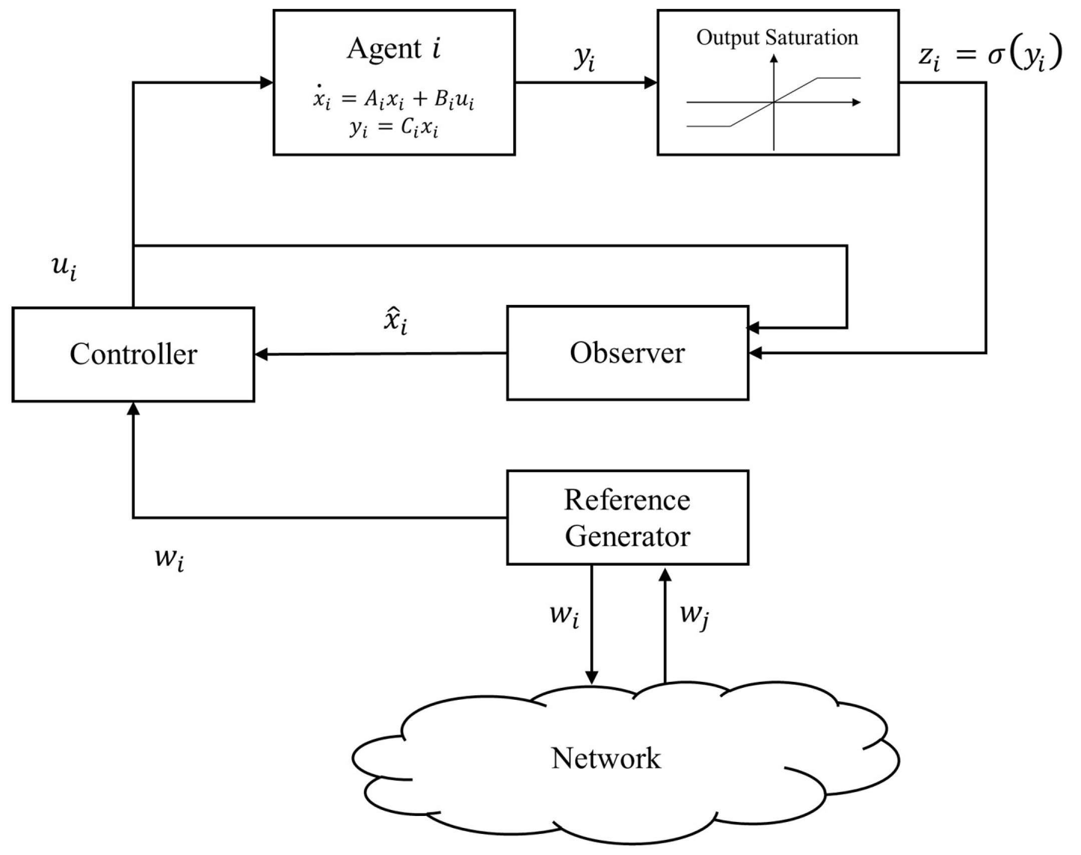
In this section, we construct the consensus algorithms for heterogeneous agents with the output saturations and consider the cases of leaderless and leader-following. The proposed algorithms are composed of three parts, as shown in Figure 1. The first part is the nonlinear observer to measure the state using the measured output, the second part is the distributed reference generator to generate the common trajectory, and the third part is the controller to track the common trajectory based on the output regulation theory.
3.1. Leaderless Case
In this subsection, we consider the output consensus without the leader agent. We propose the observer-based consensus algorithm as follows:
where and are the states of the observer and the reference generator of the ith agent, respectively; , F and are the gain matrices with compatible dimensions that will be determined later; and S, and are the constant matrices satisfying Assumption 1. Before we present our main result, we consider the following lemma [11].
Lemma 4.
Suppose that the pair is stabilizable. Then, there exists a symmetric positive-definite matrix W such that
Then, we can solve the leaderless output consensus problem from the following theorem.
Theorem 1.
- is a constant matrix such that is Hurwitz.
- is bounded such that , for , , where is the solution of the following dynamics:
Proof of Theorem 1.
To prove the consensus, we investigate the asymptotic stability of the error dynamics. Then, we first consider the reference generator (8b) and define the state vector . Then, from (8b), we have
Since the graph is undirected and connected, there exists an orthogonal matrix , such that with and [14]. Let with and with . In [12], it was shown that , , if and only if . Moreover, if , , , where is the solution of (10) [10]. Therefore, in what follows, we derive the asymptotic convergence of to the origin. After the coordinate transformation, we have
where .
We next consider the observer (8a) and the regulator (8c) and define the observer error and the regulation error as and , respectively. Then, from (5), the observer error dynamics can be written as
and, from Assumption 1, the regulation error dynamics is given by
Let , , , , , , , , , , , and . Then, from (12), (13), and (14), the overall error dynamics can be written as
It is clear that we can achieve the consensus if the error dynamics (15) is asymptotically stable, i.e., if , then , . Then, to prove the consensus, we first analyze the asymptotic convergence of and e to the origin, applying Lemma 2. We define the continuously differentiable functionV as follows:
where W is the solution of (9) in Lemma 4 and with given in Lemma 1. Let and . Then, the time-derivative of V is given by
Then, from Lemma 1 and 4, and the fact that , the time-derivative of V can be rewritten as
where we have used the fact that, for any , . Then, we have shown that is radially unbounded and , which implies that Conditions 1 and 2 in Lemma 2 hold. Then, to prove Condition 3, we define . implies , i.e., , , and , and , . Then, in the set , the error dynamics in (15) can be rewritten as
Since is Hurwitz, , we have
Moreover, implies , and, thus, from Condition 4 in Theorem 1, we have in . Therefore, there exists a finite time such that , , which gives, for , in . Then, for , the observer error dynamics can be rewritten as
Since is Hurwitz from Lemma 1, e converges to 0.
In summary, we have shown that and is a unique, asymptotically stable equilibrium point in . Therefore, according to Lemma 2, we have and , . Moreover, since is Hurwitz, the regulation error dynamics is input-to-state stable. Then, from Lemma 3, we have . Finally, we can conclude that and , , which completes the proof. □
3.2. Leader-Following Case
In this subsection, we consider the leader agent, which generates the reference trajectory. The dynamics of the leader is given by
where and are the state and output, respectively, of the leader. S and R are the constant matrices satisfying Assumption 1. Then, to achieve the consensus, we consider the following assumption to control the follower agents into the leader’s trajectory.
Assumption 4.
- is detectable.
- For the leader agent, there exists , satisfying
Then, to achieve the consensus, we propose the following consensus algorithm:
where and are the states of the observer and the reference generator of the ith follower, respectively; , F and are the gain matrices with compatible dimensions that will be determined later; and and are the solution of linear matrix equations in Assumption 1. We next consider the following lemma [10], which is the dual problem of Lemma 4:
Lemma 5.
Suppose that the pair is detectable. Then, there exists a symmetric positive-definite matrix W such that
Then, we can solve the leader-following output consensus from the following theorem.
Theorem 2.
Consider a group of N follower agents (1) with the leader (22). Suppose that Assumptions 1–4 hold, and there exists at least one follower that can receive the information from the leader. Then, we can achieve the leader-following output consensus using the observer-based consensus algorithm (24) if the gain matrices satisfy the following conditions:
- , where is any positive constant, and are given in (5), and is given in Lemma 1.
- , where τ is a positive constant such that , where , and the positive definite matrix W is the solution of (25) in Lemma 5.
- is a constant matrix such that is Hurwitz.
Proof of Theorem 2.
We apply the same procedure as in the proof of Theorem 1. We define the tracking error of the reference generator, the observer error and the regulation error as , , and , respectively. Then, the tracking error dynamics is given by
and, from (13) and (14), the observer error dynamics and the regulation error dynamics are given by
where we have used the fact that .
Let and , and define , and as in the proof of Theorem 1. Then, the overall error dynamics can be written as
It is clear that we can achieve the leader-following output consensus if the error dynamics (28) is asymptotically stable; i.e., if , then , . Then, to prove the consensus, we define the continuously differentiable functionV as follows:
where W is the solution of (25) and with given in Lemma 1. Let and . Then, the time-derivative of V is given by
where we have used the fact that . Then, we have shown that is radially unbounded and , which implies that conditions 1 and 2 in Lemma 2 hold. Then, to prove Condition 3, we define . implies , i.e., , , and , . Then, in , the error dynamics (28) can be rewritten as
Then, since is Hurwitz and , we have
and, thus, there exists a finite time such that , . Therefore, following the proof of Theorem 1, we can prove that e converges to 0.
In summary, we have shown that , and is a unique, asymptotically stable equilibrium point in . Therefore, according to Lemma 2, we have and , . Moreover, since is Hurwitz, the regulation error dynamics is input-to-state stable. Then, from Lemma 3, we have . Finally, we can conclude that and , , which completes the proof. □
Remark 1.
Note that Theorems 1 and 2 give the sufficient conditions to achieve the output consensus. The existence of control gains follows from Assumptions 1–4, which are the standard assumptions to achieve the consensus for the heterogeneous agents. Moreover, the control gains can be constructed from the knowledge of the system matrices except τ, which requires the global information, i.e., in Theorem 1 and in Theorem 2. However, by choosing τ as an arbitrarily large constant, the conditions can be satisfied.
4. Simulations
In this section, we present two numerical examples to demonstrate the theoretical results.
4.1. Leaderless Case
In this subsection, we consider the leaderless case with 10 agents modeled by harmonic oscillators. The dynamics of each agent is of the form (1) with, for ,
We next consider the linear matrix equations (4) in Assumption 1. The analytic solution of (4) is given in [20] as follows:
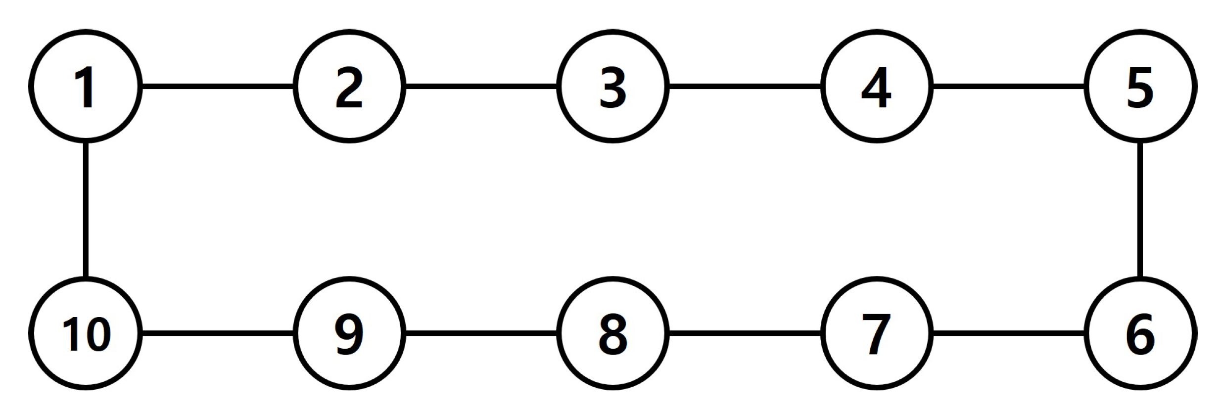
In this simulation, we assume that the communication between agents is as ring topology given in Figure 2. We consider , if and otherwise. Then, the Laplacian matrix is given by
and . We next construct the observer-based consensus algorithm (8) applying Theorem 1. From the condition 1, we choose
We next choose such that is stabilize and Lemma 4 is satisfied. Then, from the condition 2, we choose
where such that . Finally, we choose such that Condition 3 is satisfied, i.e., is Hurwitz. We conduct the simulation with the initial conditions satisfying Condition 4 as follows:
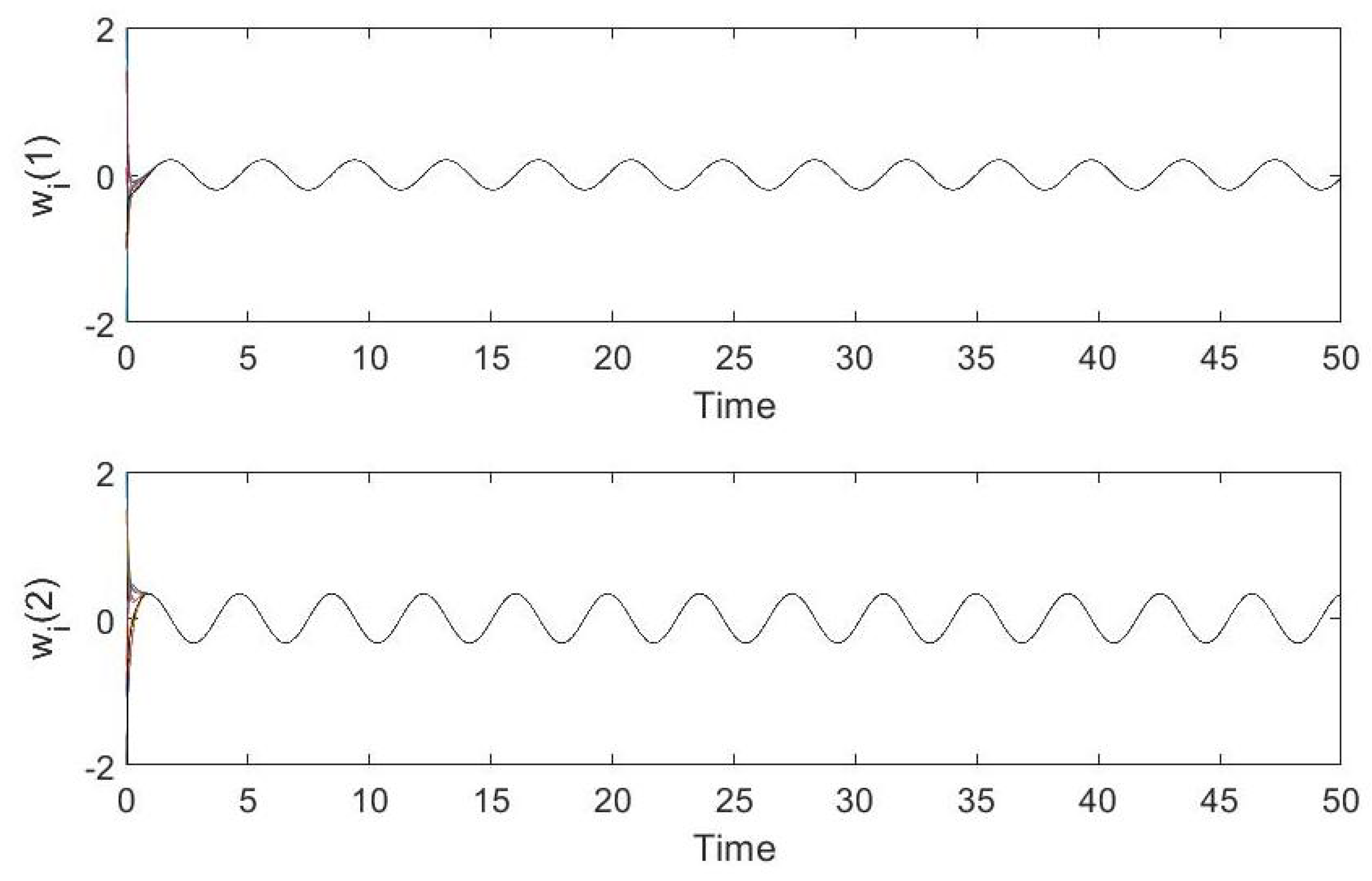
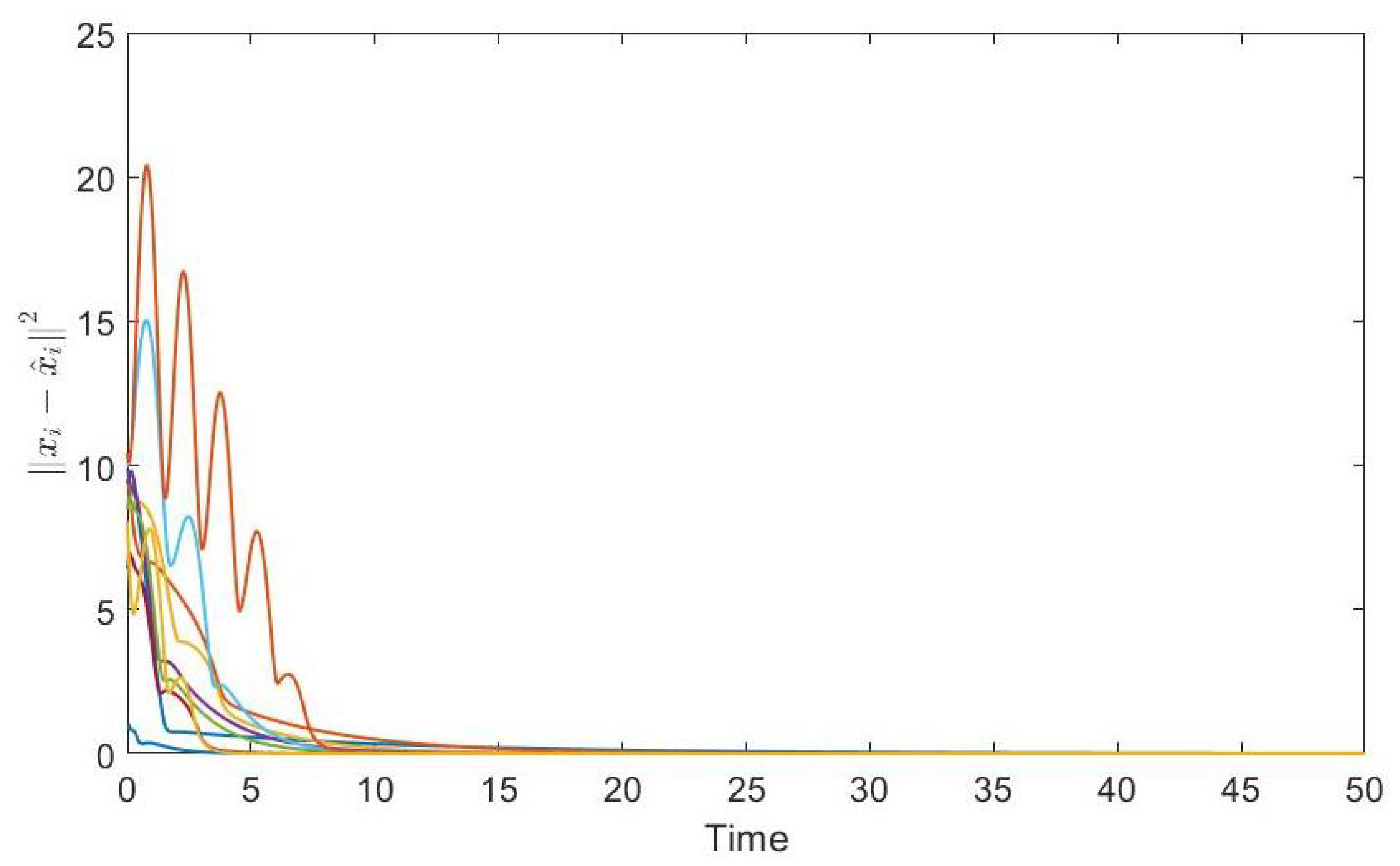
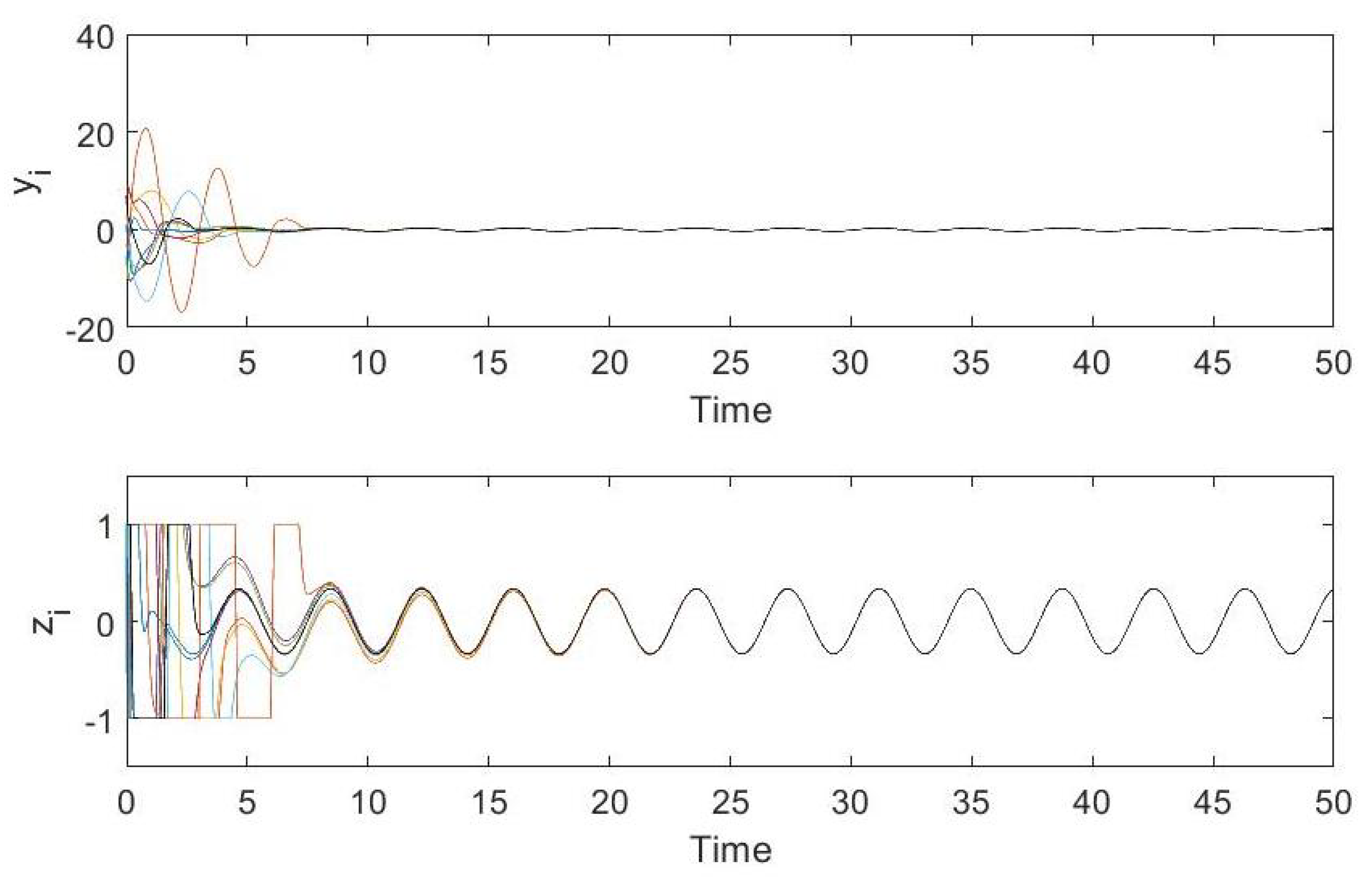
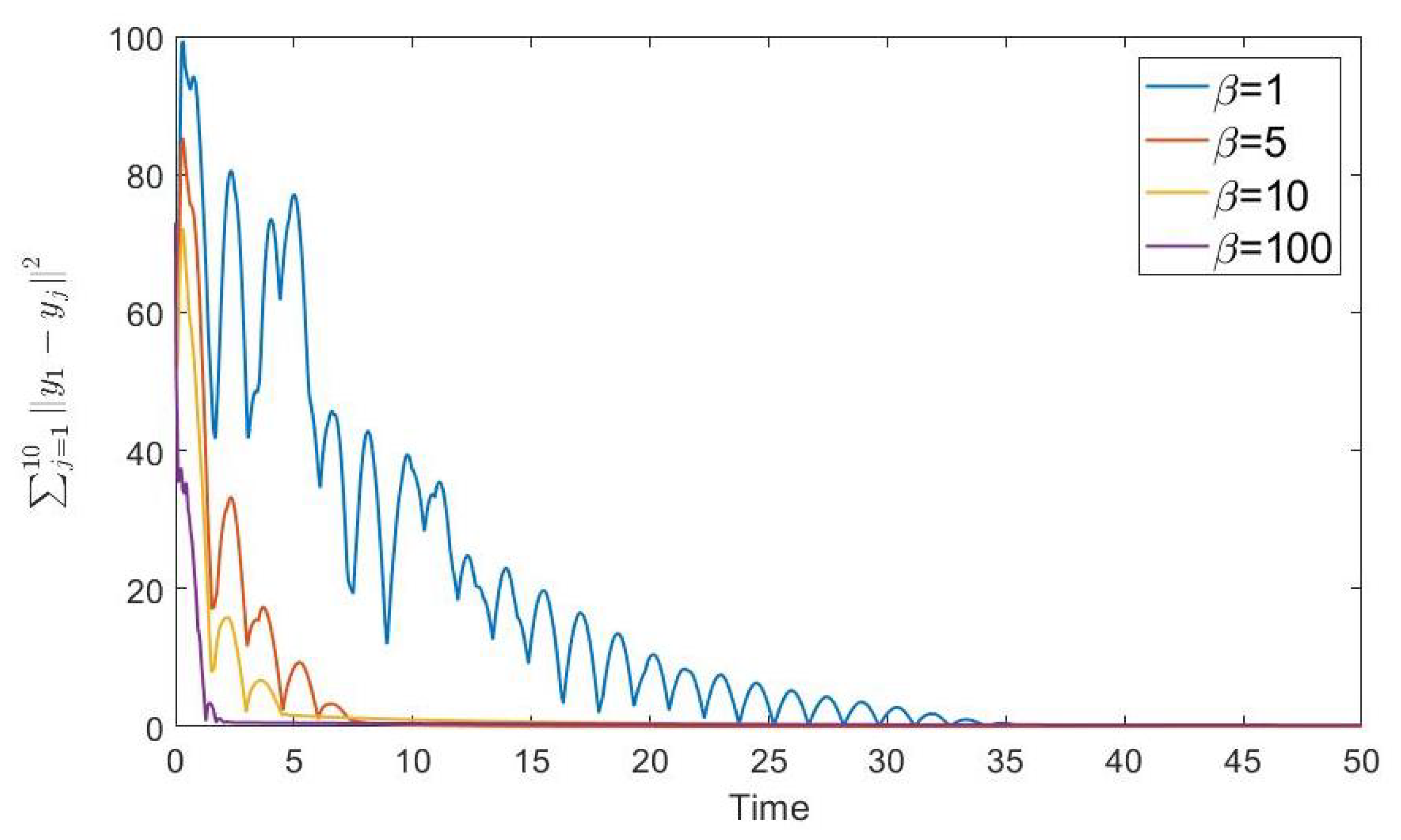
The simulation results using the proposed algorithm are shown in Figure 3, Figure 4, Figure 5 and Figure 6. Figure 3 shows the state trajectories of the reference generators. As we can see from Figure 3, the reference generators converge to the common trajectory. Figure 4 shows the square norms of the observer errors, which converge to zero. Thus, the states of the agents can be measured under the proposed nonlinear observer (8a). Figure 5 depicts the controlled and the measured output trajectories of agents. Although the measured outputs are saturated, the agents achieve the consensus under the proposed algorithm. Moreover, to investigate the effect of the control gain , we conduct the simulation with , and the square norms of the output errors between agents are shown in Figure 6. The simulation result shows that, as the control gain increases, the agents achieve a fast convergence speed.
4.2. Leader-Following Case
In this subsection, we consider a group of four agents (1), i.e., , and a leader agent (22) with [18]
which satisfies Assumption 2 and Condition 1 in Assumption 4. Then, we can choose the non-singular matrix , and the positive semi-definite matrix satisfying Lemma 1 as follows:
Moreover, by solving the linear equations in Assumption 1, we have
In this simulation, we consider the communication topology between the agents given in Figure 7. We consider , if and otherwise. Then, the Laplacian matrix is given by
and and . We next construct the observer-based consensus algorithm (24) applying Theorem 2. From Condition 1, we choose with , , and given in (42). We next choose W satisfying Lemma 5 as
Then, from Condition 2, we choose with such that . Finally, we choose the gain matrix , such that is Hurwitz
In this simulation, we choose the initial conditions of the followers as follows:
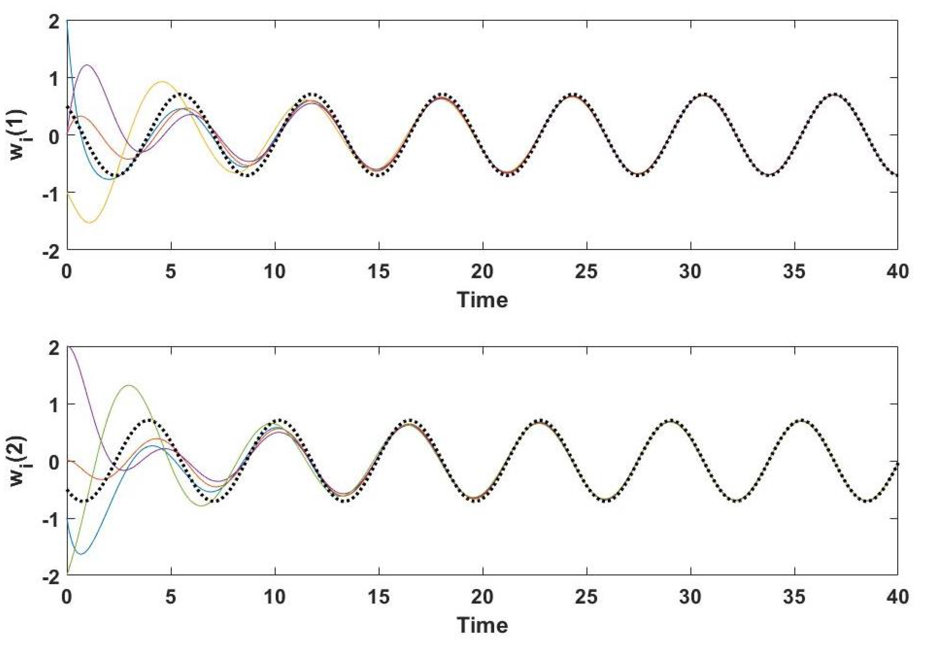
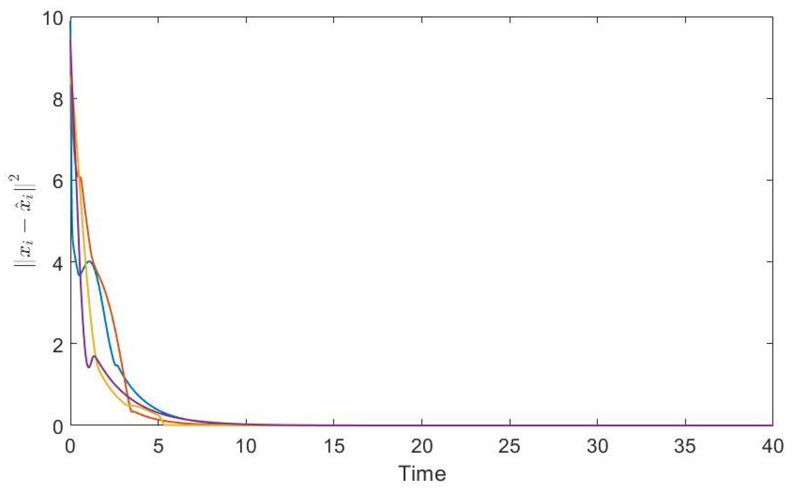
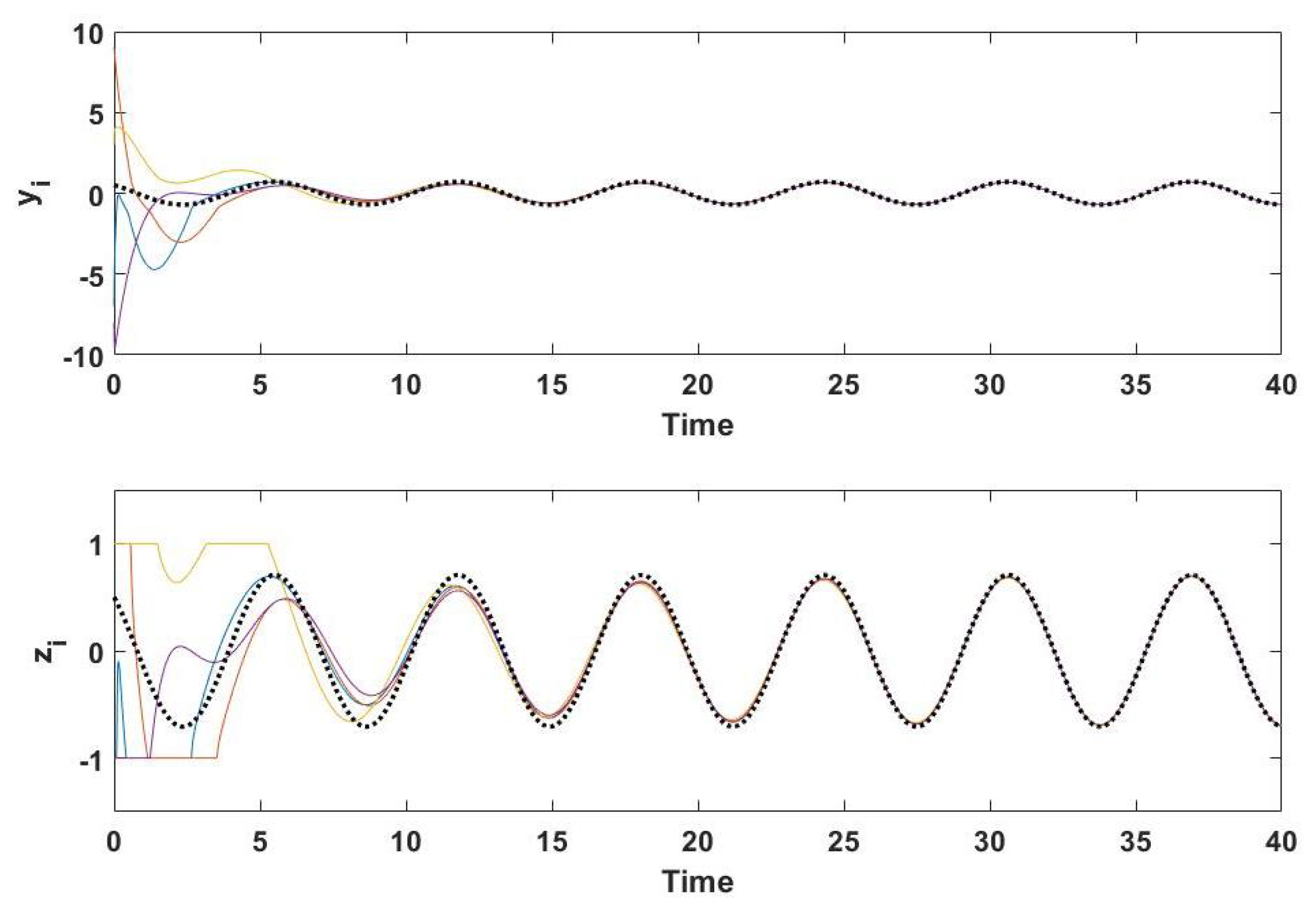
The initial condition of the leader is chosen as such that Assumption 4 is satisfied. The simulation results are given in Figure 8, Figure 9 and Figure 10. In Figure 8, the solid line shows the trajectories of the reference generators, while the dashed line shows the trajectory of the leader. It can be observed from Figure 8 that the reference generators track the leader’s trajectory. In Figure 9, we can see that the observer errors converge to zero, which means the proposed nonlinear observer (24a) performs well. Moreover, the controlled and measured output trajectories of the followers in solid line are given in Figure 10. It is clear that the followers track the leader’s trajectory in the dashed line, and, thus, the proposed algorithm solves the leader-following consensus problem.
5. Conclusions
In this paper, the output consensus problems for heterogeneous agents were studied under the output saturations. Applying the output regulation approach to solve the consensus problem, we have proposed the observer-based consensus algorithms considering leaderless and leader-following cases. Specifically, the proposed algorithm consists of three parts: the nonlinear observer, the reference generator, and the regulator. By defining the error dynamics, we have transformed the consensus problem into the stability problem of the error dynamics. Then, based on the Lasalle’s Invariance Principle and the input-to-state stability, the stability of error dynamics and the existence of the control gains have been derived under the standard assumptions for the consensus. Finally, two numerical examples have been given to demonstrate the theoretical results. Although the effect of the control gain has been investigated by simulation, the performance in a group has not been addressed. Thus, the consensus control with the performance analysis would be worthwhile for a further study. Moreover, as mentioned in Remark 1, the proposed algorithm requires global information, i.e., and . To solve this problem, the fully distributed algorithm has been widely used [14]. By using the state dependent control gain, the consensus can be solved without global information. Therefore, it would be interesting to extend the results of this paper to fully distributed consensus.
Author Contributions
Conceptualization, Y.-H.L. and G.-S.L.; methodology, Y.-H.L.; software, G.-S.L.; validation, Y.-H.L. and G.-S.L.; formal analysis, Y.-H.L. and G.-S.L.; investigation, Y.-H.L.; resources, Y.-H.L.; data curation, G.-S.L.; writing—original draft preparation, Y.-H.L.; writing—review and editing, G.-S.L.; visualization, G.-S.L.; supervision, G.-S.L.; project administration, G.-S.L.; funding acquisition, G.-S.L. All authors have read and agreed to the published version of the manuscript.
Funding
This work was supported by Gyeongsang National University Grant in 2020–2021.
Institutional Review Board Statement
Not applicable.
Informed Consent Statement
Not applicable.
Data Availability Statement
Not applicable.
Conflicts of Interest
The authors declare no conflict of interest.
References
- Ren, W.; Beard, R.W.; Atkins, E.M. Information consensus in multivehicle cooperative control. IEEE Control Syst. Mag. 2007, 27, 71–82. [Google Scholar]
- Olfati-Saber, R.; Shamma, J.S. Consensus filters for sensor networks and distributed sensor fusion. In Proceedings of the 44th IEEE Conference on Decision and Control, and the European Control Conference 2005, Seville, Spain, 12–15 December 2005. [Google Scholar]
- Lee, J.; Back, J. Robust distributed cooperative controller for dc microgrids with heterogeneous sources. Int. J. Control Autom. Syst. 2021, 19, 736–744. [Google Scholar] [CrossRef]
- Olfati-Saber, R.; Fax, J.A.; Murray, R.M. Consensus and Cooperation in Networked Multi-Agent Systems. Proc. IEEE 2007, 95, 215–233. [Google Scholar] [CrossRef] [Green Version]
- Olivares, D.; Romero, G.; Guerrero, J.A.; Lozano, R. Robustness analysis for multi-agent consensus systems with application to dc motor synchronization. Appl. Sci. 2020, 10, 6521. [Google Scholar] [CrossRef]
- Ren, W.; Atkins, E.M. Distributed multi-vehicle coordinated control via local information exchange. Int. J. Robust Nonlinear Control 2007, 17, 1002–1033. [Google Scholar] [CrossRef] [Green Version]
- Ren, W. On consensus algorithms for double-integrator dynamics. IEEE Trans. Autom. Control 2008, 58, 1503–1509. [Google Scholar] [CrossRef]
- Abdessameud, A.; Tayebi, A. On consensus algorithms design for double integrator dynamics. Automatica 2013, 49, 253–260. [Google Scholar] [CrossRef]
- Seo, J.H.; Shim, H.; Back, J. Consensus of high-order linear systems using dynamic output feedback compensator: Low gain approach. Automatica 2009, 45, 2659–2664. [Google Scholar] [CrossRef]
- Li, Z.; Duan, Z.; Chen, G.; Huang, L. Consensus of multiagent systems and synchronization of complex networks: A unified viewpoint. IEEE Trans. Circuits Syst. I Regul. Pap. 2010, 57, 213–224. [Google Scholar]
- Ni, W.; Cheng, D. Leader-following consensus of multi-agent systems under fixed and switching topologies. Syst. Control Lett. 2010, 59, 209–217. [Google Scholar] [CrossRef]
- Trentelman, H.L.; Takaba, K.; Monshizadeh, N. Robust Synchronization of Uncertain Linear Multi-Agent Systems. IEEE Trans. Autom. Control 2013, 58, 1511–1523. [Google Scholar] [CrossRef] [Green Version]
- Yu, W.; Chen, G.; Cao, M.; Kurths, J. Second-order consensus for multi-agent systems with directed topologies and nonlinear dynamics. IEEE Trans. Syst. Man Cybern. B 2010, 40, 881–891. [Google Scholar]
- Zhang, F.; Trentelman, H.L.; Scherpen, J.M.A. Fully distributed robust synchronization of networked Lur’e systems with incremental nonlinearities. Automatica 2014, 50, 2515–2526. [Google Scholar] [CrossRef]
- Liu, J.; Dai, M.-Z.; Zhang, C.; Wu, J. Edge-event-triggered synchronization for multi-agent systems with nonlinear controller outputs. Appl. Sci. 2020, 10, 5250. [Google Scholar] [CrossRef]
- Wieland, P.; Sepulchre, R.; Allgower, F. An internal model principle is necessary and sufficient condition for linear output synchronization. Automatica 2011, 47, 1068–1074. [Google Scholar] [CrossRef]
- Ma, Q.; Miao, G. Output consensus for heterogeneous multi-agent systems with linear dynamics. Appl. Math. Comput. 2015, 271, 548–555. [Google Scholar] [CrossRef]
- Han, T.; Guan, Z.-H.; Xiao, B.; Wu, J.; Chen, X. Distributed output consensus of heterogeneous multi-agent systems via an output regulation approach. Neurocomputing 2019, 360, 131–137. [Google Scholar] [CrossRef]
- Li, X.; Ma, D.; Hu, X.; Sun, Q. Dynamic event-triggered control for heterogeneous leader-following consensus of multi-agent systems based on input-to-state stability. Int. J. Control Autom. Syst. 2020, 18, 293–302. [Google Scholar] [CrossRef]
- Baldi, S.; Frasca, P. Leaderless synchronization of heterogeneous oscillators by adaptively learning the group model. IEEE Trans. Autom. Control 2020, 65, 412–418. [Google Scholar] [CrossRef] [Green Version]
- Su, H.; Chen, M.Z.; Lam, J.; Lin, Z. Semi-global leader-following consensus of linear multi-agent systems with input saturation via low gain feedback. IEEE Trans. Circuits Syst. I Regul. Pap. 2013, 60, 1881–1889. [Google Scholar] [CrossRef] [Green Version]
- Wang, X.; Su, H.; Wang, X.; Chen, G. Fully distributed event-triggered semiglobal cosnensus of multi-agent systems with input saturations. IEEE Trans. Ind. Electron. 2017, 64, 5055–5064. [Google Scholar] [CrossRef]
- Wang, B.; Chen, W.; Zhang, B. Semi-global robust tracking consensus for multi-agent uncertain systems with input saturation via metamorphic low-gain feedback. Automatica 2019, 103, 363–373. [Google Scholar] [CrossRef]
- Zhao, Z.; Lin, Z. Global leader-following consensus of a group of general linear systems using bounded controls. Automatica 2016, 68, 294–304. [Google Scholar] [CrossRef]
- Xie, Y.; Lin, Z. Global optimal consensus for multi-agent systems with bounded controls. Syst. Control Lett. 2017, 102, 104–111. [Google Scholar] [CrossRef]
- Shi, L.; Li, Y.; Lin, Z. Semi-global leader-following output consensus of heterogeneous multi-agent systems with input saturation. Int. J. Robust Nonlinear Control 2018, 28, 4916–4930. [Google Scholar] [CrossRef]
- Lim, Y.-H.; Ahn, H.-S. Semiglobal consensus of heterogeneous multiagent systems with input saturations. Int. J. Robust Nonlinear Control 2018, 28, 5652–5664. [Google Scholar] [CrossRef]
- Liu, K.; Gu, H.; Wang, W.; Lu, J. Semiglobal consensus of a class of heterogeneous multi-agent systems with saturation. IEEE Trans. Neural Netw. Learn. Syst. 2020, 31, 4946–4955. [Google Scholar] [CrossRef]
- Wang, Q.; Sun, C. Conditions for consensus in directed networks of agents with heterogeneous output saturations. IET Control Theory Appl. 2016, 10, 2119–2127. [Google Scholar] [CrossRef]
- Lim, Y.-H.; Ahn, H.-S. Consensus with output saturations. IEEE Trans. Autom. Control 2016, 62, 5388–5395. [Google Scholar] [CrossRef]
- Wang, Q. Scaled consensus of multi-agent systems with output saturation. J. Frankl. Inst. 2017, 354, 6190–6199. [Google Scholar] [CrossRef]
- Lim, Y.-H.; Lee, G.-S. Observer-based distributed consensus algorithm for multi-agent systems with output saturations. J. Inf. Commun. Converg. Eng. 2019, 17, 167–173. [Google Scholar]
- Hilhorst, G. Stabilisation of Linear Time-Invariant Systems Subject to Output Saturation. Master’s Thesis, University of Twente, Enschede, The Netherlands, 2011. [Google Scholar]
- Khalil, H.K. Nonlinear Systems, 3rd ed.; Prentice-Hall PTR: Upper Saddle River, NJ, USA, 2002. [Google Scholar]
Figure 1.
Block diagram of agent i with the observer-based consensus algorithm.

Figure 2.
Communication topology between 10 agents.

Figure 3.
The state trajectories of the reference generators using the proposed algorithm (8).
Figure 3.
The state trajectories of the reference generators using the proposed algorithm (8).

Figure 4.
The observer errors using the proposed algorithm (8).
Figure 4.
The observer errors using the proposed algorithm (8).

Figure 5.
The trajectories of the controlled outputs and the measured outputs using the proposed algorithm (8).
Figure 5.
The trajectories of the controlled outputs and the measured outputs using the proposed algorithm (8).

Figure 6.
The output errors between agents using the proposed algorithm (8) with .
Figure 6.
The output errors between agents using the proposed algorithm (8) with .

Figure 7.
Communication topology between four agents, labeled by , and a leader, labeled by 0.

Figure 8.
The state trajectories of the reference generators (solid line) and the leader (dashed line) using the proposed algorithm (24).
Figure 8.
The state trajectories of the reference generators (solid line) and the leader (dashed line) using the proposed algorithm (24).

Figure 9.
The observer errors using the proposed algorithm (24).
Figure 9.
The observer errors using the proposed algorithm (24).

Figure 10.
The trajectories of the controlled outputs (solid line), the measured outputs (solid line), and the leader’s output (dashed line) using the proposed algorithm (24).
Figure 10.
The trajectories of the controlled outputs (solid line), the measured outputs (solid line), and the leader’s output (dashed line) using the proposed algorithm (24).

Publisher’s Note: MDPI stays neutral with regard to jurisdictional claims in published maps and institutional affiliations. |
© 2021 by the authors. Licensee MDPI, Basel, Switzerland. This article is an open access article distributed under the terms and conditions of the Creative Commons Attribution (CC BY) license (https://creativecommons.org/licenses/by/4.0/).
Share and Cite
MDPI and ACS Style
Lim, Y.-H.; Lee, G.-S. Observer-Based Consensus Control for Heterogeneous Multi-Agent Systems with Output Saturations. Appl. Sci. 2021, 11, 4345. https://doi.org/10.3390/app11104345
AMA Style
Lim Y-H, Lee G-S. Observer-Based Consensus Control for Heterogeneous Multi-Agent Systems with Output Saturations. Applied Sciences. 2021; 11(10):4345. https://doi.org/10.3390/app11104345
Chicago/Turabian StyleLim, Young-Hun, and Gwang-Seok Lee. 2021. "Observer-Based Consensus Control for Heterogeneous Multi-Agent Systems with Output Saturations" Applied Sciences 11, no. 10: 4345. https://doi.org/10.3390/app11104345
Note that from the first issue of 2016, this journal uses article numbers instead of page numbers. See further details here.