
Wall Thinning Assessment for Ferromagnetic Plate with Pulsed Eddy Current Testing Using Analytical Solution Decoupling Method

1
College of Automation Engineering, Nanjing University of Aeronautics and Astronautics, Nanjing 210016, China
2
School of Mechanical Science & Engineering, Huazhong University of Science and Technology, Wuhan 430074, China
*
Author to whom correspondence should be addressed.
Appl. Sci. 2021, 11(10), 4356; https://doi.org/10.3390/app11104356
Submission received: 27 March 2021
/
Revised: 7 May 2021
/
Accepted: 7 May 2021
/
Published: 11 May 2021
(This article belongs to the Topic Metallurgical and Materials Engineering)
Abstract
:The wall-thinning measurement of ferromagnetic plates covered with insulations and claddings is a main challenge in petrochemical and power generation industries. Pulsed eddy current testing (PECT) is considered as a promising method. However, the accuracy is limited due to the interference factors such as lift-off and cladding. In this study, by decoupling analytic solution, a feature only sensitive to plate thickness is proposed. Based on the electromagnetic waves reflection and transmission theory, cladding-induced interference is firstly decoupled from the analytical model. Moreover, by using the first integral mean value theorem, interferences of insulation and the lift-off are decoupled, too. Hence, the method is proposed by calculating Euclidean distances between the normalized detection signal and normalized reference signal as the feature to assess wall thinning. Its effectiveness under various conditions is examined and results show that the proposed feature is only sensitive to the ferromagnetic plate thickness. Finally, the experiment is carried on to verify this method practicable.
1. Introduction
Ferromagnetic plates are commonly used materials in petrochemical and power generation industries. Wall thinning is one critical threat to ferromagnetic plates. It is caused by corrosion under insulation (CUI), flow accelerated corrosion (FAC), or liquid droplet impingement (LDI), and severely affects the structural strength and integrity of ferromagnetic plates [1,2]. Therefore, wall thinning assessment is important. The thickness measurement is an essential early warning method. Whereas the ferromagnetic plates in petrochemical and power generation applications are always wrapped with insulations and externally protected metal claddings. Therefore, it is challenging for the commonly used methods, such as ultrasonic testing (UT) and eddy current testing (ECT), to determine the plate thickness without removing the insulations and claddings [3]. Pulsed eddy current testing (PECT) provides a possible solution. PECT involves excitation by a square-wave pulse rather than a sinusoidal waveform. So, it contains a variety of frequency components and large driving electric currents, which allows for non-contact remote sensing [4,5]. Therefore, it could be used to measure the thickness of ferromagnetic plates covered with insulations and claddings.
The PECT signal is a complicated coupling response related to many factors [6,7]. including ferromagnetic plate thicknesses, insulations, claddings, and lift-offs (distance from the sensor to the cladding), etc. Thus, decoupling the ferromagnetic plate thickness from other factors is a key problem in PECT. Some features have been proposed to evaluate the plate thickness. Waidelich et al. [8] proved that the peak value, time to zero-crossing (TZC), and lift-off intersection (LOI) of the differential PECT signal could be used to evaluate the thickness. Bieber et al. [9] verified these features experimentally and further proposed that the peak value was proportional to the metal loss extent, and the TZC contained information regarding the flaw depth. Fan et al. [10] showed that the LOI point could be adjusted by varying the rising time of pulse excitation, which was beneficial to extend the measurement range and to increase the measurement sensitivity. Smith and Hugo [11] used the time-to-peak to characterize defects and structural variations in aging aircraft structures, showing that the time-to-peak and defect depth exhibited a quadratic relationship. Xu et al. [12] compared the time-to-peak and peak value for wall thinning assessment, and found that the time-to-peak was superior to the peak value due to its linear relationship with wall thickness. Tian et al. [13] proposed the rising point to identify and quantify the defects, and proved that the rising point was related to the propagation time of electromagnetic waves in metallic plates. However, these features [8,9,10,11,12,13] are all obtained by analyzing special points in PECT signals, they are easily affected by the confounding factors. For example, the peak value [8,9] and the time-to-peak [11,12] are related to the cladding thicknesses [12], and the rising point [13] relates to the sensor lift-off [14].
Cheng [15] discussed magnetic field variation by using an anisotropic magneto-resistive (AMR) sensor embedded differential detector, showing that the signal decay behavior was only relevant to the pipe wall thickness over a limited time after switching off the excitation current. Li et al. [16] studied the magnetic flux change with variable pulsed width excitation, demonstrating that the slope of the relative increase in magnetic flux and pulse width could be used to evaluate the ferromagnetic plate thickness. However, the feature proposed by Cheng [15] cannot be obtained when a coil is used as a detector, which limits its application. The slope of the relative increase in magnetic flux and pulse width [16] are complicated. Therefore, an efficient and easy-to-use signal feature, which is sensitive only to the ferromagnetic plate thickness, is still needed.
In this study, a feature only sensitive to plate thickness is proposed through electromagnetic waves theory. The electromagnetic waves theory has been used for PECT analysis in some researches. Waidelich [8] propose features, such as the peak value, TZC, and the LOI, by considering the wave produced by the square-wave pulse was a plane wave. However, the model [8] was imprecise, because the wave produced by the square-wave pulse could be regarded as a plane wave only if the transmission coil radius or plate thickness was sufficiently large [17,18]. Then, Dodd–Deeds model was used to obtain the analytical solution of the PECT problem [19,20]. Fan et al. [21] reinterpreted the model using the reflection-transmission theory, which provided it a clearly physical meaning. According to the previous studies, the reflection and transmission of electromagnetic waves in the ferromagnetic plates covered with insulations and claddings are further studied, and by decoupling the analytical solution, a feature which is only sensitive to the thickness is introduced in this study.
The rest of this paper is organized as follows: Part II describes the modeling of the insulated ferromagnetic plate, and the theoretical analysis for decoupling the interference caused by claddings, insulations, and lift-offs. In Part III, the similarity measurement based feature is presented, and in part IV, the validity of the feature is proved by experimental study. In part V, the performances of the feature are examined under various conditions. Finally, a brief conclusion is provided in part V.
2. Theoretical Analysis
In this section, the PECT analytical model and its solution are described firstly, and then, the reflection and transmission of the electromagnetic waves is discussed to decouple the cladding-induced interference. Moreover, influences of insulations and lift-off effects to the PECT signal are studied by using the first integral mean value theorem.
2.1. Solution for PECT Analytical Model
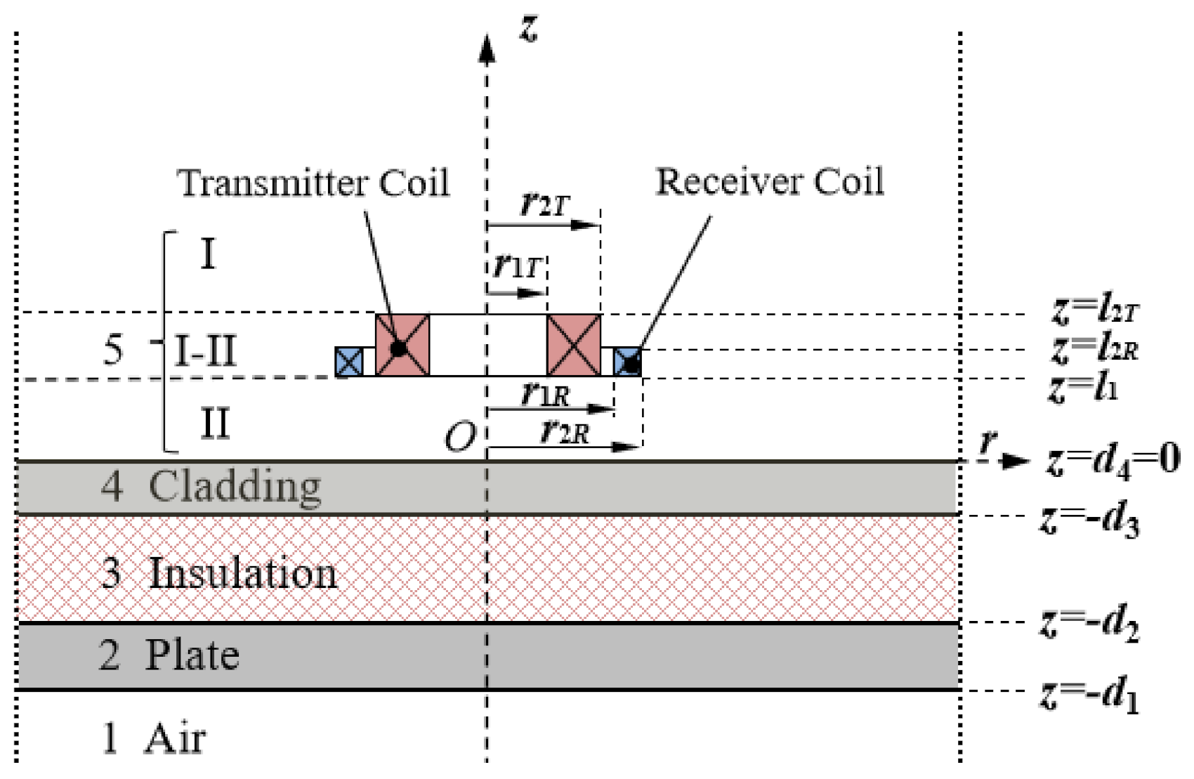
As shown in Figure 1, a ferromagnetic plate with an insulation and a cladding is modeled as a four-layered structure for simplicity. Layers from bottom to top represent the air, the plate, the insulation, and the cladding, successively. The layer over the cladding is layer 5, and it is divided into three subregions. The sensor consisting of transmitter and receiver coils with rectangular cross-sections is in section I-II.
According to the reflection and transmission theory of electromagnetic waves, the expression of the reflection coefficient at the interface between layers k + 1 and k is:
where βk = (α2 + jωμ0μrkσk)1/2; μrk and σk are the relative magnetic permeability and electrical conductivity of layer k, respectively; j is the imaginary unit; ω is the angular frequency of the sinusoidal harmonic; μ0 is the permeability of vacuum; α can be understood as a wavenumber [5].
Received waves are the superposition of reflection waves from multiple interfaces, thus some scholars have defined a generalized reflection coefficient to represent the superposition of reflection waves [20,21,22]. The generalized reflection coefficient R′k + 1,k is defined as the ratio of the electromagnetic wave reflected at all the interfaces between the layer 1 and k + 1 to the electromagnetic wave incident from the layer k + 1 to k. It satisfies the recursive Equation (2).
with the initial condition R′2,1(α) = R2,1(α), where (dk−1 − dk) denotes the thickness of layer k.
R′5,4(α) is the generalized reflection coefficient of the four-layered structure which could be derived:
For each frequency component, the induced voltage in the receiver coil could be deduced based on the Dodd–Deeds model [23]:
where I(ω) is the amplitude of the harmonic excitation current; S(α) is the spatial frequency spectra of the sensor which gives the amplitude of the contributions as a function of α [21].
where Int(x1, x2) = xJ1(x)dx, J1(x) denotes the first-order Bessel function; l1 is the sensor lift-off, e−2αl1 is the lift-off coefficient; n is the coil turns number, r1, r2, and (l2 − l1) are the inner radius, outer radius, and the coil height, respectively; the subscripts T and R label the transmitter and receiver coils, respectively.
Substituting Equations (1)–(3) and Equation (5) into Equation (4), the induced voltage in frequency domain can be obtained. As the square-wave excitation current of PECT could be theoretically represented by superimposing a series of sinusoidal harmonics in the frequency domain. The PECT signal could be derived from a sum of harmonic responses in the frequency domain through using an inverse discrete Fourier transform (IDFT), the expression of which is
where ts denotes the s-th point in time, m denotes the m-th sinusoidal harmonic, N is the number of sampling point.
2.2. Decoupling the Cladding-Induced Interference
As shown in Equation (1), the solution of the PECT signal is mainly depended on three parameters: the sensor spatial frequency spectra, S(α); generalized reflection coefficient of the four-layered structure, R′5,4(α); and lift-off coefficient, e−2αl1. According to Equations (1)–(3), R′5,4(α) is determined by the ferromagnetic plate, the insulation and the cladding. e−2αl1 is related to the sensor lift-off. Then through analyzing R′5,4(α) and e−2αl1, the interference factors could be discussed. As R′5,4(α) indicates that the interference caused by the cladding and the insulation are coupled with the ferromagnetic plate, thus, R′5,4(α) is discussed firstly.
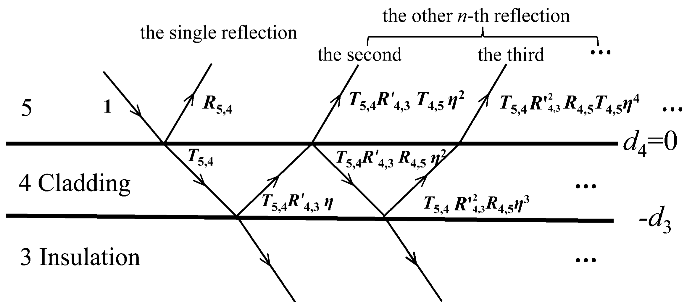
R′5,4 (α) is the result of the ratio between the amplitudes of the reflected wave and the incident wave [22]. It essentially indicates the electromagnetic wave propagation in the four-layered structure. As shown in Figure 2, the amplitude of the incident wave in layer 5 is set to 1, and then R5,4 and T5,4 denote the single reflection and transmission from the interface between layers 5 and 4, respectively. In addition, as the thickness of layer 4 is finite, there are multiple reflections and transmissions in layer 4, for example T5,4R′4,3η, T5,4R′4,3R4,5η2, T5,4R4,5η3, … And T5,4R′4,3T4,5η2, T5,4R4,5T4,5η4, …are the related multiple reflections in layer 5.
Figure 2 indicates that R′5,4 (α) is the sum of the single reflection coefficient and the other n-th reflections whose general expression is T5,4R′(n − 1)4,3R(n − 2)4,5T4,5η2(n − 1). Wherein T5,4 = 1 + R5,4, R4,5 = −R5,4, η = e-β4(d3 − d4). To explain this more clearly, R′5,4 (α) in (3) could be rewritten as follows:
where the first term is the single reflection coefficient, and the second term is the sum of the other n-th reflections.
According to Equation (1), R5,4(α) = (αμr4 − β4)/(αμr4 + β4), wherein β4 = (α2 + jωμ0μr4σ4)1/2. It indicates that R5,4 (α) is only related to the cladding material. Therefore, R5,4(α) could be regarded as part of the cladding-induced interference. In addition, Waidelich demonstrated that the amplitude of the first reflection was much larger than that of the other reflections [8]. Therefore, the interference caused by R5,4(α) is significant.
To further decouple the interference caused by the cladding, the electromagnetic wave propagation in layers 2 and 3 is studied with the same method, and the generalized reflection coefficient R′4,3 is rewritten as follows:
where the first term, R4,3(α), could be expressed as R4,3(α) = (μr3β4-μr4β3)/(μr3β4 + μr4β3). As the insulation is always composed of non-conducting material, such as rock wool or foamed glass, then μr3 = 1, β3 = α. Thus, R4,3(α) could be rewritten as R4,3(α) = (β4 − μr4α)/(β4 + μr4α) = −R5,4(α). Therefore, R4,3(α) is also related only to the cladding material.
If Equation (8) is completely substituted into Equation (7), the expressions of R′5,4(α) will become very complicated, which is not conducive to decoupling. So, Equation (8) is firstly substituted into the first R′4,3(α) in Equation (7), then R′5,4(α) becomes:
where, (d3 − d4) is the thickness of the cladding, R5,4(α) and R4,3(α) are only related to cladding material. The R′4,3(α) that still remains in Equation (9) can be approximated by R4,3(α), since the first reflection was much stronger than that of the other reflections, and R4,3(α) significantly influences the value of R′4,3(α). Thus, the equations in the first line of Equation (9) is only related to the material and thickness of the cladding.
Substituting Equation (9) into Equation (4), ΔU could be divided into two terms:
where according to Equation (9), ΔU1 is only related to the cladding, and it is the cladding-induced interference signal. ΔU2 contains the information regarding the ferromagnetic plate thickness, which is the desired signal. In addition, according to Equations (1)–(3), ΔU2 is also influenced by the cladding, while the interference is negligible. This will be demonstrated in Section 4.
2.3. Influence Analysis of Insulation and Lift-Off
Based on the analysis above, ΔU2 is the signal which the cladding-induced interference has been decoupled. However, as shown in Equation (10), ΔU2 is still affected by the insulation thickness, (d2 − d3), and the sensor lift-off, l1. Therefore, methods for reducing these interferences should be further studied.
As β3 = α, R4,3(α) = −R5,4(α), ΔU2 in Equation (10) could be rewritten as follows:
where the parameter Coef(α) is used for simplicity.
As the commonly used cladding is 0.3−0.7 mm thick, the commonly used insulation is 40 mm to a few hundred mm thick, and the sensor lift-off is a few mm [24]. Thus, the cladding thickness, (d3 − d4), is much smaller than the sum of the sensor lift-off and the insulation thickness, (l1 + d2 − d3). Therefore, e−2α(l1 + d2 − d3)−2β4(d3 − d4) could be approximated by e−2α(l1 + d2 − d3). Then, Equation (11) could be rewritten as follows:
In Equation (13), as S(α)R′3,2(α) × Coef(α) is continuous in the range [0, ∞], and e−2α(l1 + d2 − d3) is continuous with its values always greater than zero. Thus, the first integral mean value theorem [25] could be used, and Equation (13) becomes:
where ε is a value between 0 and ∞.
Calculating e−2α(l1 + d2 − d3) dα gives e−2α(l1 + d2 − d3) dα =1/2(l1 + d2 − d3), thus (14) could be rewritten as follows:
Because jπωμ0I(ω) and S(ε)R′3,2(ε) × Coef(ε) are independent of (d2 − d3) and l1, ΔU2 is inversely proportional to (l1 + d2 − d3). Therefore, the relationship that ΔU2 is approximately inversely proportional to the sensor lift-off and the insulation is obtained.
3. Similarity Measurement Based Feature
As indicated above, the original signal, ΔU, could be decomposed into two terms ΔU1 and ΔU2, where ΔU1 is the cladding-induced interference, and ΔU2 contains the information regarding the plate thickness. For ΔU1, differential methods or similarity measurement methods could be used to eliminate it. However, the differential method is always used as a pre-processing method [8,9,10,11,12]. It cannot obtain the thickness measurement feature directly. Therefore, the similarity measurement method is selected herein. In addition, as ΔU2 is approximately inversely proportional to the insulation thickness and sensor lift-off, (l1 + d2 − d3) can be reduced by dividing two signals. Normalization method is used to eliminate the influence of interfering factors. Then a feature based on the similarity measurement of the normalized PECT signal is proposed in this study.
The similarity of the signals is always measured by the distance information. It could be calculated through the Euclidean distance, angular separation, correlation coefficient et al. In this paper, the Euclidean distance is used. Then, the feature could be calculated as follows:
where Dis is the Euclidean distance, ΔUnorr is the normalized reference signal, and ΔUnor is the normalized calibration signal or the detection signal. Moreover, the reference signal is the signal of the defect-free plate, the calibration signal is the signal of the plate with a known thickness, and the detection signal is the signal of the detected plate.
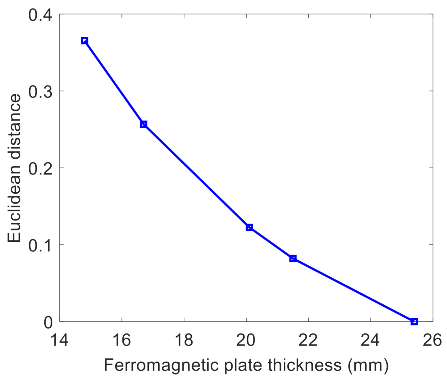
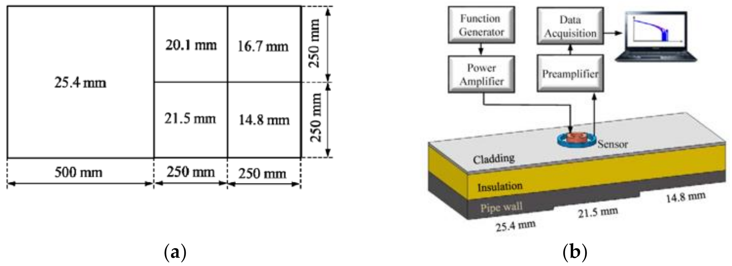
To examine the feature detailly, a 16 Mn steel step wedge plate is used. The thicknesses of the 16 Mn steel step wedge plate are 25.4 mm, 21.5 mm, 20.1 mm, 16.7 mm, and 14.8 mm. The thicknesses of the insulation and the cladding located above the plate are 40 mm and 0.5 mm, respectively. The cladding is composed of galvanized steel sheet (GS cladding). The sensor parameters are listed in Table 1. The lift-off of the sensor is 5 mm, and the amplitude, duty cycle, and period of the square-wave current are 4 A, 50%, and 1 s, respectively. Moreover, the signals of the 16Mn steel plate are calculated based on the analytical model described in Section 2.1. In the calculation, the relative magnetic permeability and conductivity of the 16Mn steel plate are 500 and 1.6 MS/m, respectively, and those of the GS cladding are 300 and 2.0 MS/m, respectively. As ΔU shown in Equation (1) is expressed as an integral of Bessel functions which is cumbersome and complex, the truncated region eigenfunction expansion (TREE) method presented in [26] is applied to calculate the signals.
The calculated normalized signal obtained from the 25.4 mm thick plate is used as the reference signal ΔUnorr, and those obtained from the 21.5 mm, 20.1 mm, 16.7 mm, and 14.8 mm thick plates are used as the calibration signals ΔUnor. Substituting ΔUnorr and ΔUnor into Equation (15), Dis are obtained. The results are shown in Figure 3. It shows that the plate thickness is monotonically related to the Euclidean distances, then it can be used for thickness measurement.
4. Experimental Study
Experimental study is conducted to further discuss the feature. Figure 4 illustrates the experimental set-up. Similar to the set-up shown in Section III, a 16 Mn steel step wedge plate with thicknesses of 25.4 mm, 21.5 mm, 20.1 mm, 16.7 mm, and 14.8 mm is used, of which the reference thickness is 25.4mm, and plates with other thickness are used to simulate the uniform wall thinning. A 40 mm thick plastic plate and a 0.5 mm thick galvanized steel sheet are attached on the 16 Mn steel plate to simulate the insulation and cladding, respectively. A sensor with the parameters shown in Table 1 is placed over the cladding. The sensor lift-off is 5 mm. A square-wave voltage signal is generated by a function generator, and subsequently converted to a current signal and amplified using a power amplifier. The amplified square-wave current signal is provided to the transmitter coil. The induced voltage of the receiver coil is amplified by a preamplifier, then digitized using a data acquisition card. A computer is used to display the detection signal. The amplitude, duty cycle, and period of the square-wave current are the same as the ones provided in Section 3.
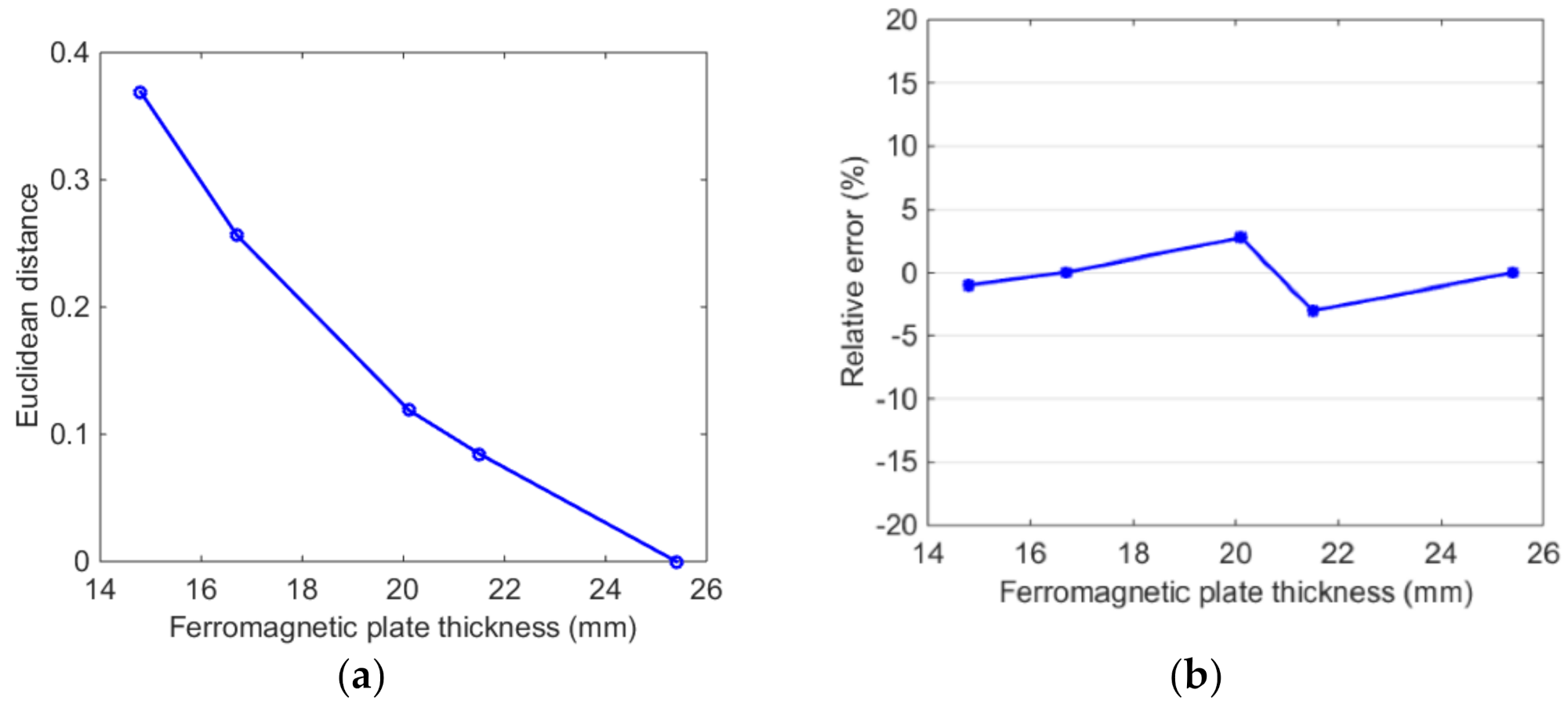
All the normalized experimental signals can be obtained by dividing each signal with its own maximum value, and are substituted into Equation (16), where the reference signal ΔUnorr is obtained from the 25.4 mm thick plate, while each ΔUnor can be obtained from plates with other thicknesses. The obtained Euclidean distances are presented in Figure 5a, and the errors between the experimental and theoretical results are shown in Figure 5b. As shown in Figure 5b, the maximum relative error is less than 5.0%, which indicates the Euclidean distance obtained by the analytical model is quite accurate. Therefore, the Euclidean distance obtained experimentally is replaced by those calculated from the analytical model in Section 5.
Furthermore, to illustrate that the feature is viable for thickness measurement, two detection signals with the real thicknesses of 23.5 mm and 18.4 mm are provided. The Euclidean distances between the detection and reference signals are 0.0353 and 0.1820, respectively. The signals obtained from 21.5 mm, 20.1 mm, 16.7 mm, and 14.8 mm thick plates are used as calibration signals, and fitting the curve of the Euclidean distances and the calibration thicknesses with a second order polynomial, a calibration equation is obtained as follows:
where x denotes the Euclidean distance, and (d1 − d2) is the ferromagnetic plate thickness.
Substituting the Euclidean distances of the detection signals into Equation (17), the calculated thicknesses are 23.6 mm and 18.3 mm, respectively. The relative errors between calculated and real thicknesses are 0.42% and 0.54%, respectively. This indicates that the feature is feasible for the ferromagnetic plate thickness assessment.
5. Discussion
To demonstrate that the proposed feature is independent of confounding factors, such as the cladding, the insulation, and the sensor lift-off, changes in the feature with the confounding factors are discussed. The plates thicknesses examined in this section are 25.4 mm, 23.5 mm, 21.5 mm, 20.1 mm, 18.4 mm, 16.7 mm, and 14.8 mm. The other calculation parameters are the same as those in Section 3, and for the convenience of comparison, only the curves of the Euclidean distances with the plate thicknesses are displayed.
5.1. Variation in Cladding Parameters
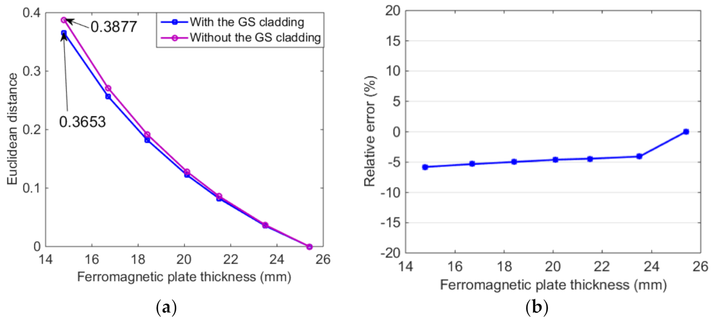
Firstly, the Euclidean distances—thicknesses curves under different cladding materials and thickness are discussed. Figure 6a is the Euclidean distances—thicknesses curves with and without the GS cladding, and Figure 6b is the errors between them. As shown in Figure 6b, the maximum error is 5.78%. It could be concluded that the feature is helpful to reduce the cladding-induced interference. This result is consistent with the analysis in Section 2.
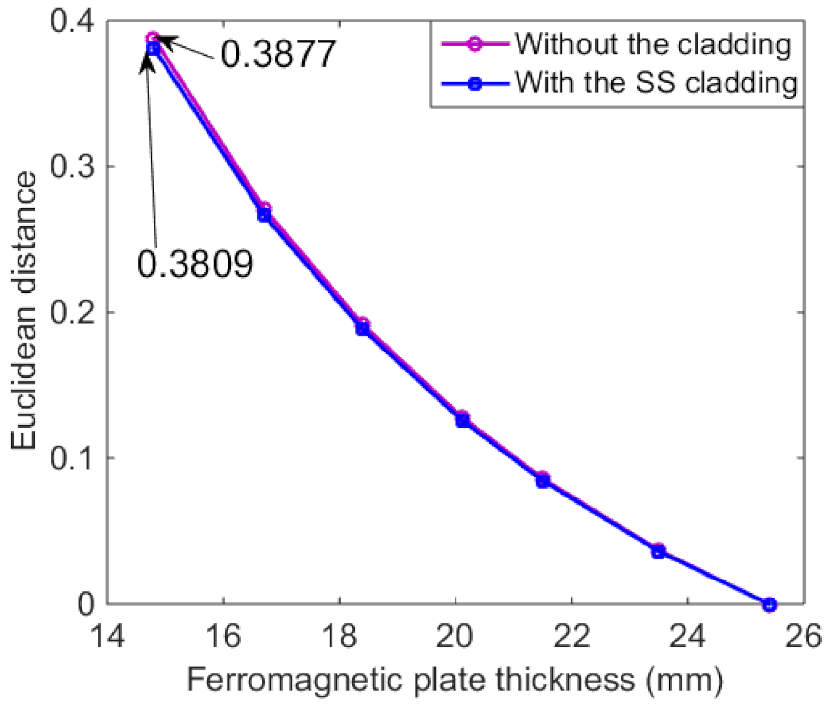
Furthermore, except for the GS cladding, a stainless-steel sheet cladding (SS cladding) is also commonly used in petrochemical and power generation applications. Then, performances of features under SS cladding are studied. Figure 7 shows features obtained with and without a 0.5 mm thick SS cladding. They are calculated through the analytical mode by setting the relative magnetic permeability and conductivity of the SS cladding to 1 and 1.35 MS/m, respectively. As shown in Figure 7, for the SS cladding, the maximum differences in Euclidean distance could be calculated by (0.3877–0.3809)/0.3877 = 1.8%. This indicates that the similarity measurement based feature is also available for SS cladding. Thus, the feature is insensitive to cladding materials.
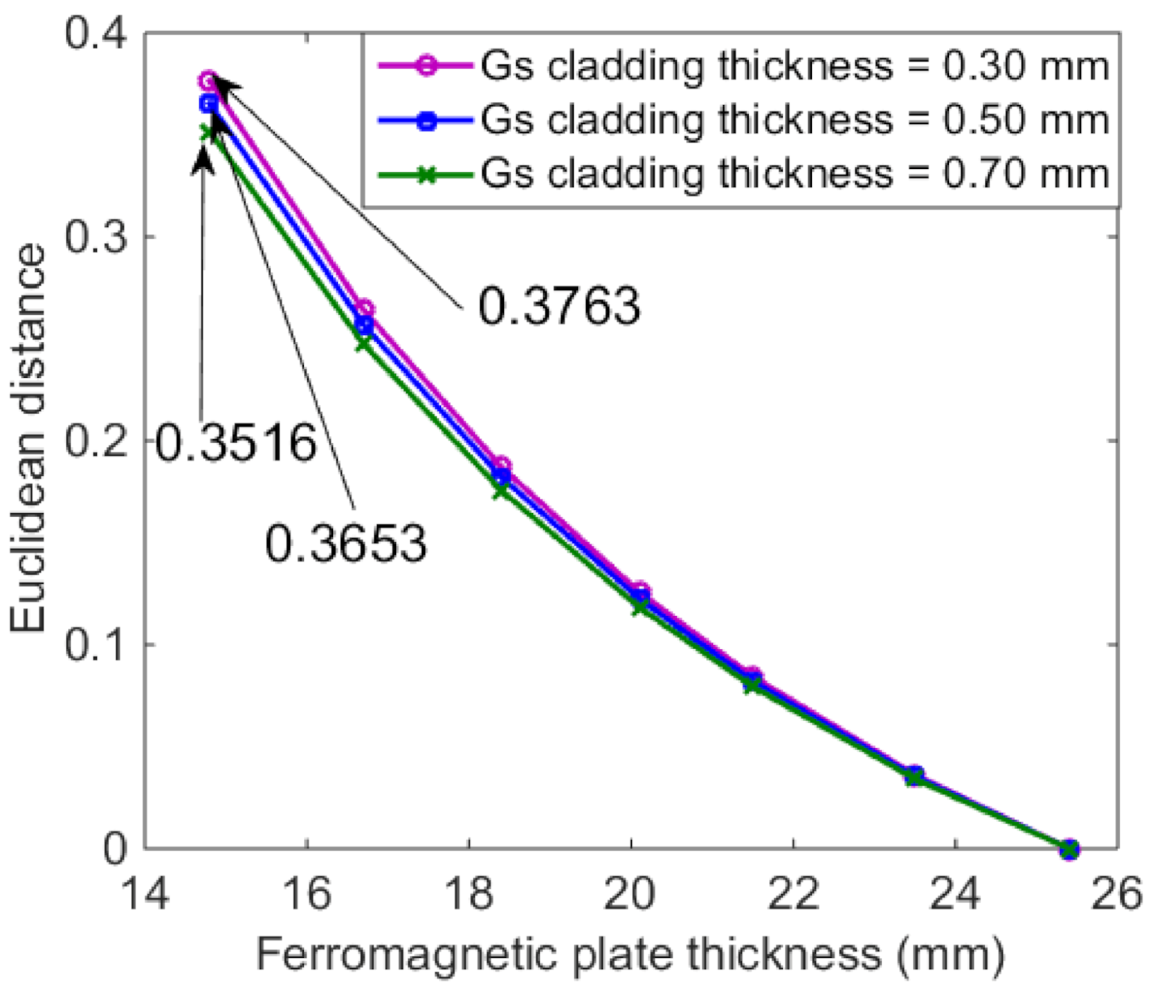
In addition, except for the cladding materials, features with different cladding thicknesses are also analyzed. According to a previous study [24], the designed cladding thicknesses are always between 0.3 and 0.7 mm, so 0.3 mm, 0.5 mm, and 0.7 mm thick claddings are examined in this study. Moreover, as the difference in Euclidean distances obtained with and without the GS cladding is larger, the GS cladding materials is used herein. Figure 8 shows the Euclidean distances with different GS cladding thicknesses. The maximum relative errors of the Euclidean distances obtained from the 0.3 mm and 0.5 mm thick cladding is calculated as (0.3763 − 0.3653)/0.3653 = 3.01%, and that for the 0.7 mm and 0.5 mm thick cladding is calculated as (0.3516 − 0.3653)/0.3653 = 3.75%. They are both small, which indicates that the Euclidean distance is independent of the cladding thickness.
In conclusion, the similarity measurement based feature is insensitive to the cladding materials and the thicknesses.
5.2. Variation in Sensor Lift-Off and Insulation Thicknesses
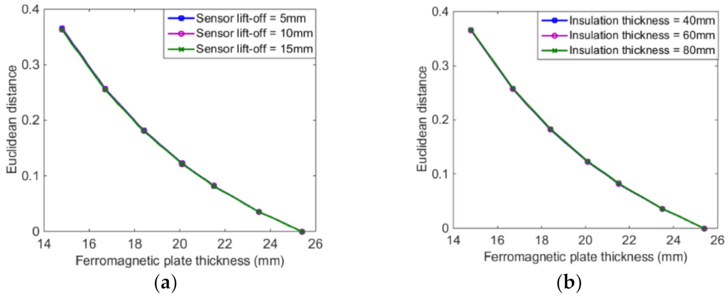
As the interference caused by the sensor lift-off could be easily masked as a defect signal. To improve the thickness assessment accuracy, the feature change with the lift-off variation is investigated. Figure 9a shows Euclidean distances obtained with 5 mm, 10 mm, and 15 mm sensor lift-offs. The Euclidean distances under different lift-offs are basically overlapped. Therefore, the Euclidean distance is independent of the sensor lift-off.
In addition, insulation thickness variations caused by installation irregularities or external forces could also affect the thickness assessment accuracy. Thus, the influence of insulation thicknesses on the Euclidean distances is examined. Figure 9b shows the Euclidean distance under different insulation thicknesses. The curves obtained with 40 mm, 60 mm, and 80 mm thick insulation are approximately overlapped, which indicates that the Euclidean distance is also independent of insulation thickness.
In conclusion, the similarity measurement based feature is independent of the sensor lift-off and the insulation thickness.
6. Conclusions
This study proposes an efficient and easy-to-use feature for the thickness assessment of ferromagnetic plates covered with claddings and insulations. The feature is obtained by decoupling the analytical solution, thus is only sensitive to the plate thickness, unaffected by other interference factors. Firstly, the insulated ferromagnetic plate is modeled as a four-layered structure, its solution provides a basis for the theoretical analysis. Secondly, by analyzing the electromagnetic wave propagation in the four-layered structure through reflection and transmission theory, the cladding-induced interference is successfully decoupled from the PECT signal. In addition, by using the first integral mean value theorem, the inversely proportional relationship between the PECT signal and the insulation thickness as well as the sensor lift-off is deduced. Thirdly, the similarity measurement based feature is proposed for thickness assessment. A 16Mn steel step plate is used as an example to study the performance of the feature. Results show the proposed feature is sensitive only to the plate thickness, and it is independent of the interference factors, including the cladding material and thickness, the sensor lift-off, and the insulation thickness.
The feature proposed in this paper is based on the similarity measurement, which effectively suppresses some interference factors. However, to eliminate the influence of environmental noises, new features shall be found based on fuzzy similarity measures to further improve the thickness assessment accuracy [27,28]. The method proposed in this paper will contribute for PECT application in ferromagnetic plate detection. Further study will include the studies for other materials and defects assessment.
Abbreviations
| Acronym | Full Name |
| PECT | Pulsed Eddy Current Testing |
| CUI | Corrosion Under Insulation |
| FAC | Flow Accelerated Corrosion |
| LDI | Liquid Droplet Impingement |
| UT | Ultrasonic Testing |
| ECT | Eddy Current Testing |
| TZC | Time to Zero-Crossing |
| LOI | Lift-Off Intersection |
| AMR | Anisotropic Magneto-Resistive |
| IDFT | Inverse Discrete Fourier Transform |
| TREE | Truncated Region Eigenfunction Expansion |
| GS | Galvanized Steel |
| SS | Stainless Steel |
Author Contributions
Conceptualization, methodology, and writing—original draft preparation, Q.Z.; writing—review and editing, X.W. All authors have read and agreed to the published version of the manuscript.
Funding
This work was supported by the National Key Research and Development Program of China, grant number 2017YFF0209701, the National Natural Science Foundation of China, grant number 61903193 and China Postdoctoral Science Foundation, grant number 2020M671476.
Institutional Review Board Statement
Not applicable.
Data Availability Statement
No new data were created or analyzed in this study. Data sharing is not applicable to this article.
Conflicts of Interest
The authors declare no conflict of interest.
References
- Li, P.; Xian, S.; Wang, K.; Zhao, Y.; Zhang, L.; Chen, Z.; Curimatid, T.; Takaki, T. A novel frequency-band-selecting pulsed eddy current testing method for the detection of a certain depth range of defects. NDT E Int. 2019, 107, 102154. [Google Scholar] [CrossRef]
- Bajracharya, S.; Sasaki, E.; Tamura, H. Numerical study on corrosion profile estimation of a corroded steel plate using eddy current. Struct. Infrastruct. Eng. 2019, 15, 1151–1164. [Google Scholar] [CrossRef]
- Chen, X.; Lei, Y. Time-domain analytical solutions to pulsed eddy current field excited by a probe coil outside a conducting ferromagnetic pipe. NDT E Int. 2014, 68, 22–27. [Google Scholar] [CrossRef]
- Xu, Z.; Zhu, J. Measurement of accumulated height of exfoliated oxide scales in austenitic boiler tubes using pulsed eddy current testing. Russ. J. Nondestruct. 2020, 56, 350–360. [Google Scholar] [CrossRef]
- Fu, F.; Bowler, J. Transient eddy-current driver pickup probe response due to a conductive plate. IEEE Trans. Magn. 2006, 42, 2029–2037. [Google Scholar] [CrossRef]
- Ge, J.; Yang, C.; Wang, P.; Shi, Y. Defect Classification Using Postpeak Value for Pulsed Eddy-Current Technique. Sensors 2020, 20, 3390. [Google Scholar] [CrossRef]
- Xie, S.; Zhang, L.; Zhao, Y.; Wang, X.; Kong, Y.; Ma, Q.; Chen, Z.; Uchimoto, T.; Takagi, T. Features extraction and discussion in a novel frequency-band-selecting pulsed eddy current testing method for the detection of a certain depth range of defects. NDT E Int. 2020, 111, 102211. [Google Scholar] [CrossRef]
- Waidelich, D.L. Pulsed Eddy Currents Gauge Plating Thickness. Electronics, University of Missouri Bulletin. 1956. Available online: https://hdl.handle.net/10355/64151 (accessed on 27 March 2021).
- Bieber, J.A.; Tai, C.C.; Moulder, J.C. Quantitative assessment of corrosion in aircraft structures using scanned pulsed eddy current. Rev. Progress Quant. Nondestruct. Eval. 1988, 17A, 315–322. [Google Scholar] [CrossRef] [Green Version]
- Wen, D.; Fan, M.; Cao, B.; Ye, B. Adjusting LOI for Enhancement of Pulsed Eddy Current Thickness Measurement. IEEE Trans. Instrum. Meas. 2019, 69, 521–527. [Google Scholar] [CrossRef]
- Smith, R.A.; Hugo, G.R. Deep corrosion and crack detection in aging aircraft using transient eddy-current NDE. In Proceedings of the 5th Joint NASA/FAA/DoD Conference on Aging Aircraft, Orlando, FL, USA, 10 September 2001. [Google Scholar]
- Xu, Z.; Wu, X.; Li, J.; Kang, Y. Assessment of wall thinning in insulated ferromagnetic pipes using the time-to-peak of differential pulsed eddy-current testing signals. NDT E Int. 2012, 51, 24–29. [Google Scholar] [CrossRef]
- Tian, G.Y.; Sophian, A. Defect classification using a new feature for pulsed eddy current sensors. NDT E Int. 2004, 38, 77–82. [Google Scholar] [CrossRef]
- Van Den Berg, S.M. Modelling and Inversion of Pulsed Eddy Current Data; Delft University of Technology: Delft, The Netherlands, 2003; pp. 31–38. [Google Scholar]
- Cheng, W. Pulsed Eddy Current Testing of carbon steel pipes’ wall-thickness through insulation and cladding. J. Nondestruct. Eval. 2012, 31, 215–224. [Google Scholar] [CrossRef]
- Li, J.; Wu, X.J.; Zhang, Q.; Sun, P.F. Pulsed eddy current testing of ferromagnetic specimen based on variable pulse width excitation. NDT E Int. 2015, 69, 28–34. [Google Scholar] [CrossRef]
- Mottl, Z. The quantitative relations between true and standard depth of penetration for air-cored probe coils in eddy current testing. NDT E Int. 1990, 23, 11–18. [Google Scholar] [CrossRef]
- Beissner, R.E.; Rose, J.H.; Nakagawa, N. Pulsed eddy current method: An overview. Rev. Prog. Quant. Nondestruct. 1999, 18, 469–475. [Google Scholar] [CrossRef]
- Zhang, Q.; Wu, X. Study on the Shielding Effect of Claddings with Transmitter–Receiver Sensor in Pulsed Eddy Current Testing. J. Nondestruct. Eval. 2019, 38, 99. [Google Scholar] [CrossRef]
- Fan, M.; Huang, P.; Ye, B.; Hou, D.; Zhang, G.; Zhou, Z. Analytical modeling for transient probe response in pulsed eddy current testing. NDT E Int. 2009, 42, 376–383. [Google Scholar] [CrossRef]
- De Haan, V.O.; de Jong, P.A. Analytical expressions for transient induction voltage in a receiving coil due to a coaxial transmitting coil over a conducting plate. IEEE Trans. Magn. 2004, 40, 371–378. [Google Scholar] [CrossRef]
- Chew, W.C. Waves and Fields in Inhomogeneous Media; IEEE Press: New York, NY, USA, 1995; Available online: https://cds.cern.ch/record/1480882 (accessed on 27 March 2021).
- Dodd, C.V.; Deeds, W.E. Analytical solutions to eddy current probe coil problems. J. Appl. Phys. 1968, 39, 2829–2838. [Google Scholar] [CrossRef] [Green Version]
- General Administration of Quality Supervision, Inspection and Quarantine of the People’s Republic of China, Ministry of Housing and Urban-Rural Development of the People’s Republic of China. GB 50264-97 Design Code for Insulation Engineering of Industrial Equipment and Pipe; Standards Press of China: Beijing, China, 1997.
- Thomas, G.B.; Finney, R.L.; Weir, M.D.; Giordano, F.R. Thomas’ Calculus; Addison-Wesley Press: New Jersey, NJ, USA, 2003; Available online: www.pearsonhighered.com (accessed on 27 March 2021).
- Theodoulidis, T.; Kriezis, E. Series expansions in eddy current nondestructive evaluation models. J. Mater. Process. Technol. 2005, 161, 343–347. [Google Scholar] [CrossRef]
- Versaci, M.; Morabito, F.C. Image Edge Detection: A New Approach Based on Fuzzy Entropy and Fuzzy Divergence. Int. J. Fuzzy Syst. 2021, 1–19. [Google Scholar] [CrossRef]
- Singh, S.; Ganie, A.H. Applications of picture fuzzy similarity measures in pattern recognition, clustering, and MADM. Expert Syst. Appl. 2020, 168, 114264. [Google Scholar] [CrossRef]
Figure 1.
Schematic of a sensor over a four-layered structure.

Figure 2.
The reflections and transmissions in layers 4 and 5.

Figure 3.
Euclidean distances under different plate thicknesses from analytical calculations.

Figure 4.
Experimental set-up for PECT: (a) The 16Mn steel step wedge plate. (b) experimental schematic diagram.
Figure 4.
Experimental set-up for PECT: (a) The 16Mn steel step wedge plate. (b) experimental schematic diagram.

Figure 5.
Experiment results: (a) Euclidean distances. (b) relative error of analytical calculations to experiment.
Figure 5.
Experiment results: (a) Euclidean distances. (b) relative error of analytical calculations to experiment.

Figure 6.
(a) Euclidean distances obtained with and without the GS cladding. (b) associated relative error.
Figure 6.
(a) Euclidean distances obtained with and without the GS cladding. (b) associated relative error.

Figure 7.
Euclidean distances obtained with and without the SS cladding.

Figure 8.
Variations of Euclidean distances due to different GS cladding thicknesses.

Figure 9.
Euclidean distances. (a) under different sensor lift-offs. (b) under different insulation thicknesses.
Figure 9.
Euclidean distances. (a) under different sensor lift-offs. (b) under different insulation thicknesses.


Table 1.
Parameters of the sensor.
| Parameters | Transmitter Coil | Receiver Coil | ||||||
|---|---|---|---|---|---|---|---|---|
| r1T (mm) | r2T (mm) | (l2T − l1) (mm) | nT | r1R (mm) | r2R (mm) | (l2R − l1) (mm) | nR | |
| Values | 16 | 40 | 34 | 800 | 72 | 76 | 6 | 1200 |
Publisher’s Note: MDPI stays neutral with regard to jurisdictional claims in published maps and institutional affiliations. |
© 2021 by the authors. Licensee MDPI, Basel, Switzerland. This article is an open access article distributed under the terms and conditions of the Creative Commons Attribution (CC BY) license (https://creativecommons.org/licenses/by/4.0/).
Share and Cite
MDPI and ACS Style
Zhang, Q.; Wu, X. Wall Thinning Assessment for Ferromagnetic Plate with Pulsed Eddy Current Testing Using Analytical Solution Decoupling Method. Appl. Sci. 2021, 11, 4356. https://doi.org/10.3390/app11104356
AMA Style
Zhang Q, Wu X. Wall Thinning Assessment for Ferromagnetic Plate with Pulsed Eddy Current Testing Using Analytical Solution Decoupling Method. Applied Sciences. 2021; 11(10):4356. https://doi.org/10.3390/app11104356
Chicago/Turabian StyleZhang, Qing, and Xinjun Wu. 2021. "Wall Thinning Assessment for Ferromagnetic Plate with Pulsed Eddy Current Testing Using Analytical Solution Decoupling Method" Applied Sciences 11, no. 10: 4356. https://doi.org/10.3390/app11104356
Note that from the first issue of 2016, this journal uses article numbers instead of page numbers. See further details here.