Curve-Localizability-SVM Active Localization Research for Mobile Robots in Outdoor Environments

Abstract

Working environment of mobile robots has gradually expanded from indoor structured scenes to outdoor scenes such as wild areas in recent years. The expansion of application scene, change of sensors and the diversity of working tasks bring greater challenges and higher demands to active localization for mobile robots. The efficiency and stability of traditional localization strategies in wild environments are significantly reduced. On the basis of considering features of the environment and the robot motion curved surface, this paper proposes a curve-localizability-SVM active localization algorithm. Firstly, we present a curve-localizability-index based on 3D observation model, and then based on this index, a curve-localizability-SVM path planning strategy and an improved active localization method are proposed. Obtained by setting the constraint space and objective function of the planning algorithm, where curve-localizability is the main constraint, the path helps improve the convergence speed and stability in complex environments of the active localization algorithm. Helped by SVM, the path is smoother and safer for large robots. The algorithm was tested by comparative experiments and analysis in real environment and robot platform, which verified the improvement of efficiency and stability of the new strategy.

1. Introduction

In recent years, working environments of autonomous mobile robots have gradually expanded to outdoor scenes like wild areas for applications such as intelligent driving, power inspection, and space exploration. The basis for the robot to move and work autonomously is to obtain the environment information through sensors. Due to the diversity and complexity of these application environments, the technical difficulties and challenges for robot localization are both increasing. Concerning about that the ability for sensors to obtain information will be greatly disturbed by environmental factors, it is necessary to estimate the robot pose and observation state during actual work using map model and robot model, so as to ensure that the robot can better perform autonomous global localization according to environmental features.

The motivation for this paper comes from the outdoor localization requirements for mobile robots in complex environments. In the uneven and complex outdoor environment, the efficiency and stability of traditional localization strategies are significantly reduced, so it is necessary to consider the terrain factors, to improve the efficiency and stability of mobile robots. In this paper, a curve-localizability-SVM based on 3D OctoMap model and 3D Lidar model is proposed to estimate the relationship between the observation state and localization pose of mobile robots in the environment, thus to generate an active convergence path which is more suitable for global localization and improve the localization efficiency.

Related Work

Researches on global localization mainly focuses on the following two aspects, scene recognition and particle filtering. Observation sensors used for global localization includes visual sensors, two-dimensional(2D) laser sensors and three-dimensional(3D) lidar sensors. Vision sensors and 3D Lidar sensors are more commonly used in outdoor applications. Benefit from the feature of rich observation information, scene recognition is commonly used for visual localization, for instance, using bag of words(BOG) model and its improved method [1,2]. However, limited by the principle of visual sensors, the effect of visual localization algorithms will be greatly affected if the environment conditions such as light change. Referring to the idea of scene recognition, some researchers focused on the recognition between two frames of laser observation information by extracting and matching the features [3,4,5], so as to perform similar effects as scene recognition.

Although researchers have done a lot of work on global localization based on scene recognition, there are still some problems such as the calculation complexity of the algorithm and the stability in different environments which are difficult to be completely solved. Therefore, based on features and advantages of the laser sensor, researchers proposed a global localization strategy based on particle filter [6,7], which is also the most widely used strategy for laser localization. In order to solve the particle degradation problem of the earliest particle filter algorithm [8], researchers proposed some advanced strategies such as importance sampling and Monte Carlo method [9]. These strategies significantly improved the effects of global localization based on particle filter.

In order to improve the convergence efficiency and stability of global localization in different application scenes, Burgard proposed the concept of active localization. One of the commonly used strategy is entropy-based localization. Since entropy itself is an index for measuring uncertainty [10,11], the uncertainty of sensor observation will have a great impact on the localization process and results, Porta proposed an active global localization strategy based on entropy increment [12], which reduced the observation uncertainty of sensors by controlling the robot to move to the areas with lower entropy values in the map. Their mechanism reduces the number of particles used by the filter and also the execution time per time slice. However, the problem of entropy-based localization strategy is that the entropy value cannot accurately distinguish the different states of sensor observation. In other words, the area with the same entropy value in the environment may have very different geometric features and scene structure, and the calculation complexity will also be higher if the environment scale gets larger, which also limits the application in large scale scenes. In addition to entropy-based strategies, some researchers have used heuristic rules [13], geometric features extraction [14,15], and other methods to obtain active paths. While it remains unclear that lower limit for the number of features that have to be present in the environment and how densely these have to be placed. Based on previous research, Wang Yong proposed an active localization strategy based on 2D static localizability for mobile robots based on the 2D laser sensor model and 2D grid map model [16]. This algorithm has been proved to have high particle convergence speed and good real-time performance in indoor structured environments.

Support Vector Machine (SVM) is an excellent linear classifier, which has been used in path planning in recent years. Different obstacle points are set as +1 or −1; the optimal classification interface between different categories found by SVM can be well applied to path planning. At the same time, if these points are not linearly separable, they can be mapped to high-dimensional space by kernel function to find a suitable classification hyperplane in high-dimensional space, which may correspond to any shape curve in low dimensional space [17]. The path planning based on SVM can optimize the path plan and reduce the influence of robot size. Aguiar et al. proposed a novel solution AgRoBPP-bridge based on SVM for path planning in agricultural robots, and it demonstrated the best performance in terms of precision and computational resources consumption [18]. Xu et al. proposed a novel path planning method using SVM and Longest Accessible Path with Course Correction (LAP-CC), and simulation experiments showed that it had the advantages of simplicity, feasibility, low computational cost and good repeatability [19]. Charalampous et al. proposed a novel local path planning method based on SVM [20]. In this method, the registration of the point clouds is accomplished via the exploitation of the localization, the FPFH features and the ICP. Relying upon stereo vision and v-disparity images, the robot can safely navigate for a long distance outdoors. Tennety et al. used SVM for path planning in unknown environment [21], and proved the effectiveness of the method through experiments. Qingyang et al. proposed a method combining a basic path subdivision method for topological maps of local environments and SVM [22]. These methods are effective, but the influence of uneven ground and the limitation of grade ability are not taken into account. For example, although some slopes are not blocked by obstacles, they are still impassable for robots.

All these methods mentioned above solve some specific problems for mobile robots active localization, but it’s still difficult to satisfy the practical application needs when the scene is expanded to outdoor, uneven-ground, feature-complex environments especially wild areas. In terms of these issues of current active localization algorithms, considering that the pose, orientation and observation state of the robot on uneven ground cannot be accurately described by the three degrees of freedom(DOFs) on 2D surface, this paper proposes a curve-localizability-SVM active global localization strategy for mobile robots in outdoor environments so that the robot can autonomously choose an active path which is conducive to robot localization, and improves the efficiency and stability of global localization. The framework of our algorithm is shown in Figure 1. In the preprocessing stage, 3D OctoMap and 3D Lidar Model are used to generate curve localizability map and accessibility map. These maps will be used for path planning and tracking. In real-time stage, odometer and 3D Lidar data are used by particle filter algorithm to locate. In Section 2, we will introduce the curve localizability index. Based on this index, Section 3 will perform active localization path planning considering localizability constraint and other traditional constraints, and then propose the curve-localizability-SVM active localization strategy combining with the improved AMCL algorithm(Adaptive Monte Carlo Localization). Experimental verification and results analysis will be described in Section 4. Finally, Section 5 is the summary and prospects of this paper.

2. Curve Localizability Estimation

Wang Yong and other researchers [16] proposed a static localizability estimation method based on 2D grid map and 2D laser sensor model by introducing the concepts of Fisher information and CRB inequality of Statistics. Concerning about the states of mobile robots and the corresponding sensor model in outdoor environments with uneven ground, we extended the 2D indoor localizability index to 3D outdoor environments, and proposed a curve localizability index based on 3D OctoMap [23] and 3D Lidar sensor, which can better adapt to the observation state of robots.

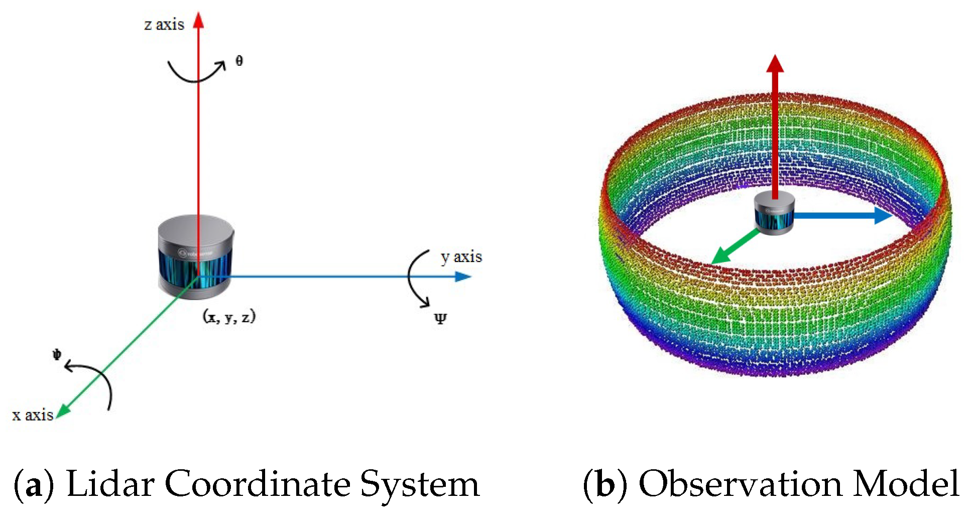
In order to make full use of the omni-direction observation characteristics of the 3D Lidar, the lidar was placed horizontally above the mobile robot, and ensured that the laser beam would not be affected by robot hardware mechanisms. On the meanwhile, for the purpose of simplifying the calculation, we assume that the mobile robot platform can be approximated as a particle, which means, the orientation of 3D Lidar remains constant if the platform is in the same position and different orientations. With this prerequisite, we can define the coordinate system of the lidar as follows.

As shown in Figure 2a, $(x,y,z)$ is the position of the 3D Lidar, and $(\phi ,\psi ,\theta )$ represents its rotation angles about the x axis, y axis, and z axis. Therefore the pose of the lidar can be expressed as $p=(x,y,z,\phi ,\psi ,\theta )$. Considering that we are using an omni-direction 3D lidar with a horizontal field of 360 degrees, the yaw angle $\theta$ has no effect on the lidar observation data, so the pose model can be simplified as $(x,y,z,\phi ,\psi )$ when calculating the curve localizability index.

We have made a strong assumption that the robot platform could be approximated as a particle before, but the effects on $\phi$ and $\psi$ of different orientations of robots cannot be ignored in real environments. According to the kinematics and dynamics characteristics of the robot platform, the maximum angle changes caused by robot hardware structures during movement were defined as $\Phi$ and $\Psi$. Therefore, we can use the 3D Lidar observation model shown as Figure 2b to traverse the interval of $[\phi -\Phi ,\phi +\Phi ]$ and $[\psi -\Psi ,\psi +\Psi ]$ for index calculation.

We define that a frame of laser observation data Z contains a set of discrete lidar points information. Suppose that the expected distance of point i in Z is $r_{iE}$, where $i=1,2,...,N$, the discrete robot localizability matrix can be defined as:

$$\widehat{J}\left(p\right)=\sum _{i=1}^N\frac{1}{{\sigma }^2}{\left(\frac{\Delta r_{iE}}{\Delta p}\right)}^T\left(\frac{\Delta r_{iE}}{\Delta p}\right)$$

(1)

Substituting the pose p of the 3D Lidar into Formula (1), we can obtain the general form of the curve localizability matrix:

$$\begin{array}{cc}\hfill & {\widehat{J}}_{curve}\left(p\right)=\sum _{i=1}^{N_1}\frac{1}{{{\sigma }_i}^2}\hfill \\ \hfill & \left[\begin{array}{cccccc}\frac{\Delta r_{iE}^2}{\Delta x^2}& \frac{\Delta r_{iE}^2}{\Delta x\Delta y}& \frac{\Delta r_{iE}^2}{\Delta x\Delta z}& \frac{\Delta r_{iE}^2}{\Delta x\Delta \phi }& \frac{\Delta r_{iE}^2}{\Delta x\Delta \psi }& \frac{\Delta r_{iE}^2}{\Delta x\Delta \theta }\\ \frac{\Delta r_{iE}^2}{\Delta x\Delta y}& \frac{\Delta r_{iE}^2}{\Delta y^2}& \frac{\Delta r_{iE}^2}{\Delta y\Delta z}& \frac{\Delta r_{iE}^2}{\Delta y\Delta \phi }& \frac{\Delta r_{iE}^2}{\Delta y\Delta \psi }& \frac{\Delta r_{iE}^2}{\Delta y\Delta \theta }\\ \frac{\Delta r_{iE}^2}{\Delta x\Delta z}& \frac{\Delta r_{iE}^2}{\Delta y\Delta z}& \frac{\Delta r_{iE}^2}{\Delta z^2}& \frac{\Delta r_{iE}^2}{\Delta z\Delta \phi }& \frac{\Delta r_{iE}^2}{\Delta z\Delta \psi }& \frac{\Delta r_{iE}^2}{\Delta z\Delta \theta }\\ \frac{\Delta r_{iE}^2}{\Delta x\Delta \phi }& \frac{\Delta r_{iE}^2}{\Delta y\Delta \phi }& \frac{\Delta r_{iE}^2}{\Delta z\Delta \phi }& \frac{\Delta r_{iE}^2}{\Delta {\phi }^2}& \frac{\Delta r_{iE}^2}{\Delta \phi \Delta \psi }& \frac{\Delta r_{iE}^2}{\Delta \phi \Delta \theta }\\ \frac{\Delta r_{iE}^2}{\Delta x\Delta \psi }& \frac{\Delta r_{iE}^2}{\Delta y\Delta \psi }& \frac{\Delta r_{iE}^2}{\Delta z\Delta \psi }& \frac{\Delta r_{iE}^2}{\Delta \phi \Delta \psi }& \frac{\Delta r_{iE}^2}{\Delta {\psi }^2}& \frac{\Delta r_{iE}^2}{\Delta \psi \Delta \theta }\\ \frac{\Delta r_{iE}^2}{\Delta x\Delta \theta }& \frac{\Delta r_{iE}^2}{\Delta y\Delta \theta }& \frac{\Delta r_{iE}^2}{\Delta z\Delta \theta }& \frac{\Delta r_{iE}^2}{\Delta \phi \Delta \theta }& \frac{\Delta r_{iE}^2}{\Delta \psi \Delta \theta }& \frac{\Delta r_{iE}^2}{\Delta {\theta }^2}\end{array}\right]\hfill \end{array}$$

(2)

According to the simplifying method of 3D Lidar pose mentioned above, and given different weights to the lidar observation data from different rotation and elevation angle, the matrix can be simplified as:

$$\begin{array}{cc}\hfill & {\widehat{J}}_{curve}\left(p\right)=\hfill \\ \hfill & \sum _{i=1}^{N_1}\frac{{\omega }_i}{{{\sigma }_i}^2}\left[\begin{array}{ccccc}\frac{\Delta r_{iE}^2}{\Delta x^2}& \frac{\Delta r_{iE}^2}{\Delta x\Delta y}& \frac{\Delta r_{iE}^2}{\Delta x\Delta z}& \frac{\Delta r_{iE}^2}{\Delta x\Delta \phi }& \frac{\Delta r_{iE}^2}{\Delta x\Delta \psi }\\ \frac{\Delta r_{iE}^2}{\Delta x\Delta y}& \frac{\Delta r_{iE}^2}{\Delta y^2}& \frac{\Delta r_{iE}^2}{\Delta y\Delta z}& \frac{\Delta r_{iE}^2}{\Delta y\Delta \phi }& \frac{\Delta r_{iE}^2}{\Delta y\Delta \psi }\\ \frac{\Delta r_{iE}^2}{\Delta x\Delta z}& \frac{\Delta r_{iE}^2}{\Delta y\Delta z}& \frac{\Delta r_{iE}^2}{\Delta z^2}& \frac{\Delta r_{iE}^2}{\Delta z\Delta \phi }& \frac{\Delta r_{iE}^2}{\Delta z\Delta \psi }\\ \frac{\Delta r_{iE}^2}{\Delta x\Delta \phi }& \frac{\Delta r_{iE}^2}{\Delta y\Delta \phi }& \frac{\Delta r_{iE}^2}{\Delta z\Delta \phi }& \frac{\Delta r_{iE}^2}{\Delta {\phi }^2}& \frac{\Delta r_{iE}^2}{\Delta \phi \Delta \psi }\\ \frac{\Delta r_{iE}^2}{\Delta x\Delta \psi }& \frac{\Delta r_{iE}^2}{\Delta y\Delta \psi }& \frac{\Delta r_{iE}^2}{\Delta z\Delta \psi }& \frac{\Delta r_{iE}^2}{\Delta \phi \Delta \psi }& \frac{\Delta r_{iE}^2}{\Delta {\psi }^2}\end{array}\right]\hfill \end{array}$$

(3)

The curve localizability index is defined by the determinant of localizability matrix:

$$l_{curve}\left(p\right)=det\left({\widehat{J}}_{curve}\left(p\right)\right)={\lambda }_x{\lambda }_y{\lambda }_z{\lambda }_{\phi }{\lambda }_{\psi }$$

(4)

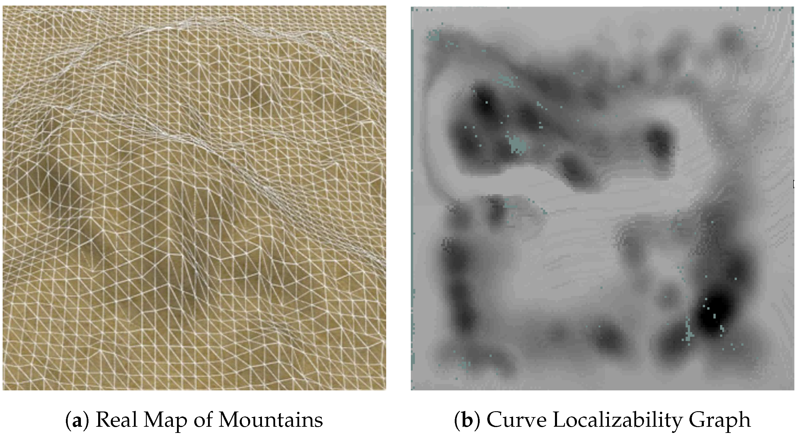
Given a 3D OctoMap, the curve localizability index of mobile robots can be calculated according to Formula (4). In order to facilitate the display and calculation needs of the following steps, the curve localizability index graph is presented in the form of a 2D gray map, as shown in Figure 3b. In this figure, the higher the gray value of the grid is, the lower the robot localizability here is.

3. Curve-Localizability-SVM Active Localization

After calculating the curve localizability index, we can generate a path which is more conducive to robot localization according to the value of localizability index and other constraints in the environment, and then combine the path with classic global localization strategies to obtain an active localization scheme which matches with scene features better.

3.1. Curve-Localizability-SVM Path Planning

Considering that in the process of active global localization, we need to generate a path which is conducive to particle convergence and robot relocation based on the coarse results of global localization, which means the selection of the path is directly related to the constraint of the curve localizability, so we propose an improved SVM algorithm for experiments, but it should be noted that our active localization strategy is not limited to one specific path planning algorithm, other suitable algorithm could be chose if necessary.

The optimal classification hyperplane found by SVM has the maximal distance between different sample classes, and the path it planned is not only smooth, but also far away from obstacles, so it can be a good path for robots. Suppose that the data sample is

$$D=\{(x_1,y_1),(x_2,y_2),...(x_m,y_m)\},y_i\in \{+1,-1\}.$$

The hyperplane can be described by the following equation:

$$w^{T}x+b=0.$$

The formula of the distance from any point x in space to the hyperplane is as follows:

$$r=\frac{\left|w^{T}x+b\right|}{w}.$$

(5)

The optimal hyperplane satisfies the following equation:

$$\underset{w,b}{max}\frac{2}{\left|\right|w\left|\right|},$$

(6)

$$s.t.y_i\left(w^T{x}_i+b\right)\ge 1,i=1,2,\dots ,n.$$

The above formula can be converted into:

$$\underset{w,b}{min}\frac{1}{2}\left|\right|\mathrm{w}\left|\right|{}^2,$$

(7)

$$s.t.y_i\left(w^T{x}_i+b\right)\ge 1,i=1,2,\dots ,n.$$

The Laplace function $L(w,b,a)$ is defined as follows:

$$L(w,b,a)=\frac{1}{2}\left|\right|\mathrm{w}\left|\right|{}^2-\sum _{i=1}^n{a}_i[y_i(w^T{x}_i+b)-1],$$

(8)

coefficient $a_i\ge 0$. The minimum problem is transformed into a dual problem of convex quadratic programming:

$$max\sum _{i=1}^n{a}_i-\frac{1}{2}\sum _{i=1}^n{a}_i{a}_j{y}_i{y}_j\left(x_i^T{x}_j\right),$$

(9)

$$s.t.y_i\left(w^T{x}_i+b\right)\ge 1,i=1,2,\dots ,n.$$

For the non-linear classificaion samples, we introduce the kernel function:

$$K(x_i,x_j)=exp(-\frac{\left|\right|x_i-x_j|{|}^2}{{\delta }^2}).$$

By solving the optimization problem:

$$max\sum _{i=1}^n{a}_i-\frac{1}{2}\sum _{i=1}^n{a}_i{a}_j{y}_i{y}_{j}K(x_i,x_j),$$

(10)

$$s.t.a_i\ge 0,i=1,2,\dots ,n,\sum _{i=1}^n{a}_i{y}_i=0.$$

Finally, the hyperplane equation is obtained:

$$f\left(x_i\right)=\sum _{j=1}^n{a}_i{y}_{i}K(x_i,x_j)+b=0.$$

(11)

To ensure that all the subsequent paths produced from SVM are connected together, we add virtual obstacles on both sides of the end point to make the next starting point connect with it. Since the SVM algorithm only considers the path length, we have to take other factors into account. In our question, the main factors that need to be considered are the length of path and curve localizability on the path, with some other traditional path planning constraints such as obstacles. We generate the active path by defining the objective function which maximize the localizability index, and taking other objects such as the length of path as the constraint conditions.

The definition of objective function is related to the value of curve localizability index, so we need to calculate the cost function of this index on the path based on the index graph firstly. Suppose P is an arbitrary path in the 2D grid map, and the grid it passes through can be defined as $g_1,g_2,g_3,...,g_n$, then the cost function of the curve localizability index on path P can be expressed as:

$$C\left(P\right)=\sum _{i=1}^n{l}_{curve}\left(p_{g_i}\right)$$

(12)

Where $C\left(P\right)$ is the total cost of path P, and $l_{curve}\left(p_{g_i}\right)$ represents the value of curve localizability index of grid $g_i$. In order to obtain the path with the highest localizability, we need to solve the following objective function:

$$P_l=\underset{P}{argmax}C\left(P\right)$$

(13)

Considering that the robot pose estimated by the state of the particles is constantly changing during the localization process, the starting point of the planning path will change according to the state of global localization or relocation. Under this premise, conventional path planning goals such as the shortest path length or shortest navigation time cannot be applied. In order to facilitate the comparison of our algorithm and other active localization strategies, we set the path length as a constant, obstacles and other accessibility factors are considered as regular constraints, so that the planned path contents the following conditions:

$$d(g_i,g_{i+1})=\sqrt{{(x_{i+1}-x_i)}^2+{(y_{i+1}-y_i)}^2+{(z_{i+1}-z_i)}^2}$$

(14)

$$D\left(P\right)=\sum _{i=1}^{n-1}d(g_i,g_{i+1})$$

(15)

$$s.t.\left\{\begin{array}{c}{g}_i\in S_{pass},\forall g_i\in P_l\\ D\left(P\right)=const\end{array}\right.$$

(16)

where $d(g_i,g_{i+1})$ is the Euclidean distance between the surface points corresponding to the grids $g_i$ and $g_{i+1}$, $S_{pass}$ is the accessible area of the map calculated by the model of robots and OctoMap offline [24], and $D\left(P\right)$ is the total length of the generated path. In the constraint space, we specify the total length of the path as a constant value and ensure that all points on the path are within the area that the robot can pass freely. Based on the above objective function and constraint conditions, we can generate a path with the highest localizability for the robot in outdoor environments.

3.2. Active Global Localization

Based on the active path generated before, we consider to optimize the active localization strategy by combining AMCL algorithm, the most commonly used global localization method. AMCL algorithm was first used for global localization in indoor scenes for mobile robots equipped with 2D laser sensors. Due to the small amount of laser observation data and limited size of scenes, it has shown good results in practical applications. However, in recent years this strategy was extended to 3D Lidar and outdoor environment, the computational complexity of the algorithm has increased significantly because of the increment of the amount of observation data and the number of particles required to estimate the pose of the robot in 3D space.

Based on the above considerations, we propose improvements in the following two aspects:

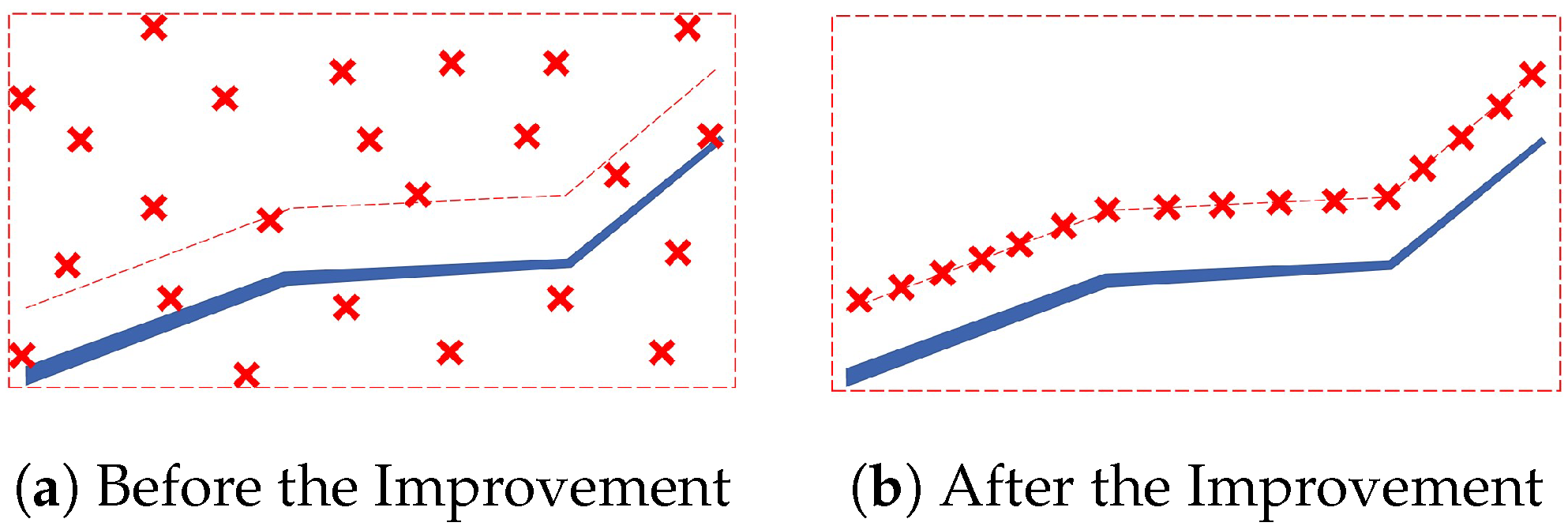
• Reduce redundant calculations. Since the movement of mobile robots in outdoor environments is constrained by the ground, we can also constrain the state of the particles within the possible curved surface of the robot pose, and re-transform the random distribution of particles in 3D space into a 2D localization problem based on motion curved surface.
• Improve localization efficiency. By pre-processing of the environment and sensor model, we can perform global localization and relocation, based on a path which can contribute to robot localization, to improve the efficiency of particle convergence.

Since the height and normal information of the ground can be obtained from 3D pointcloud map, we can determine the pose and corresponding orientation information that the robot may appear in the environment, so that the possible states of the particles can be constrained from 3D space into the motion curved surface during the initialization of global localization. Using this strategy, the number of particles that need to be injected during initialization can be significantly reduced, thereby reducing the redundant calculations. The schematic graph before and after the improvement is shown in Figure 4.

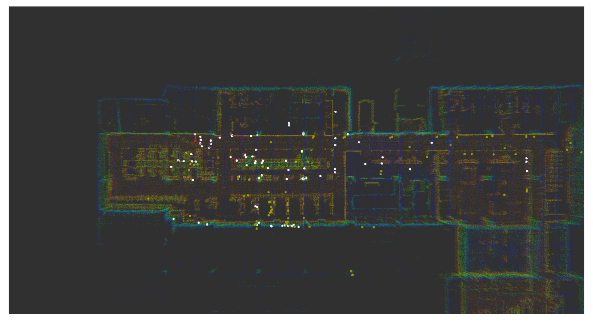
Meanwhile, considering that the robot pose estimated by particles convergence may not be the correct state, and the previous relocation strategy of AMCL by randomly injecting particles is less efficient, so we add a new relocation strategy into AMCL algorithm based on the matching result judgment between the observation data and the map, similar with pointcloud registration method of ICP algorithm. If the matching score is lower than the threshold, the relocation will start automatically.

As shown in Figure 5, the white points indicate those lidar points finding successful matches in the map, and the yellow points means that no suitable matches were found. According to the ratio of the number of white points to the total number of points in each observation frame, an appropriate threshold can be set to be used as a standard for judging the reliability of localization results. If the ratio of matching pointcloud is lower than the threshold, it means the global localization result is false, then the algorithm will enter relocation state until obtaining the correct pose.

4. Experiments and Results

This chapter is the experimental part, we will perform experimental verification and results analysis of the algorithm on the actual environment and the robot platform according to the relevant theory introduced above.

4.1. Platform and Environment

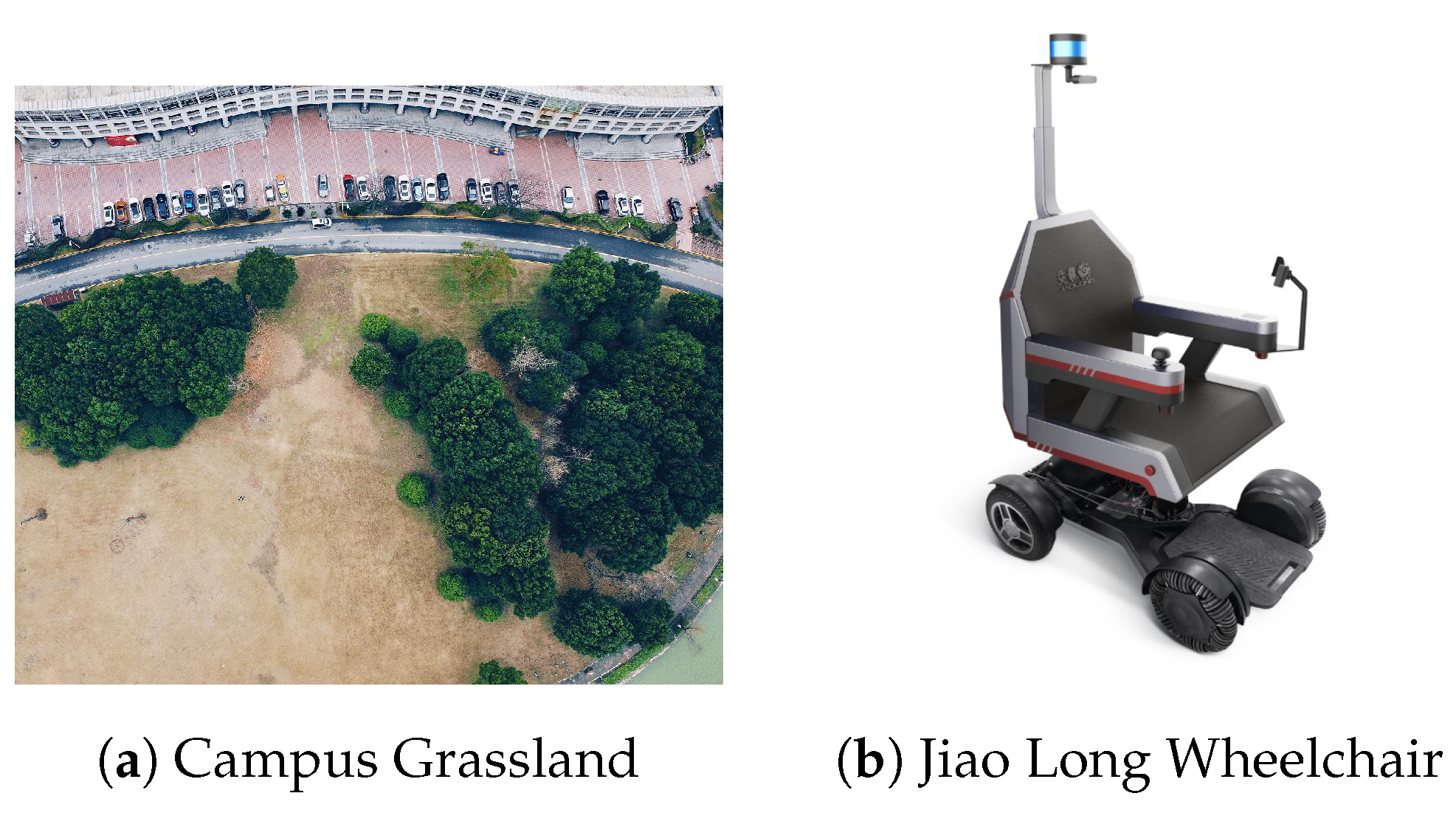
In order to reflect the effect of curve-localizability-SVM active localization algorithm, we selected a campus grassland scene with obvious slope changes for our experiments. The aerial image of the scene is shown in Figure 6a. The robot platform used in our experiment is Jiao Long Intelligent Wheelchair platform as shown in Figure 6b and main sensors include Rslidar RS-LIDAR-16 3D Lidar Sensor, Inertial Measurement Unit(IMU), and Odometer. The performance and observation principle of RS-LIDAR-16 is basically the same as VLP-16. The industrial computer of this intelligent wheelchair is equipped with Intel Core i7-8550U 1.8GHz CPU and 16G memory, our algorithms are running under the ROS Kinetic System.

4.2. Experiments and Analysis

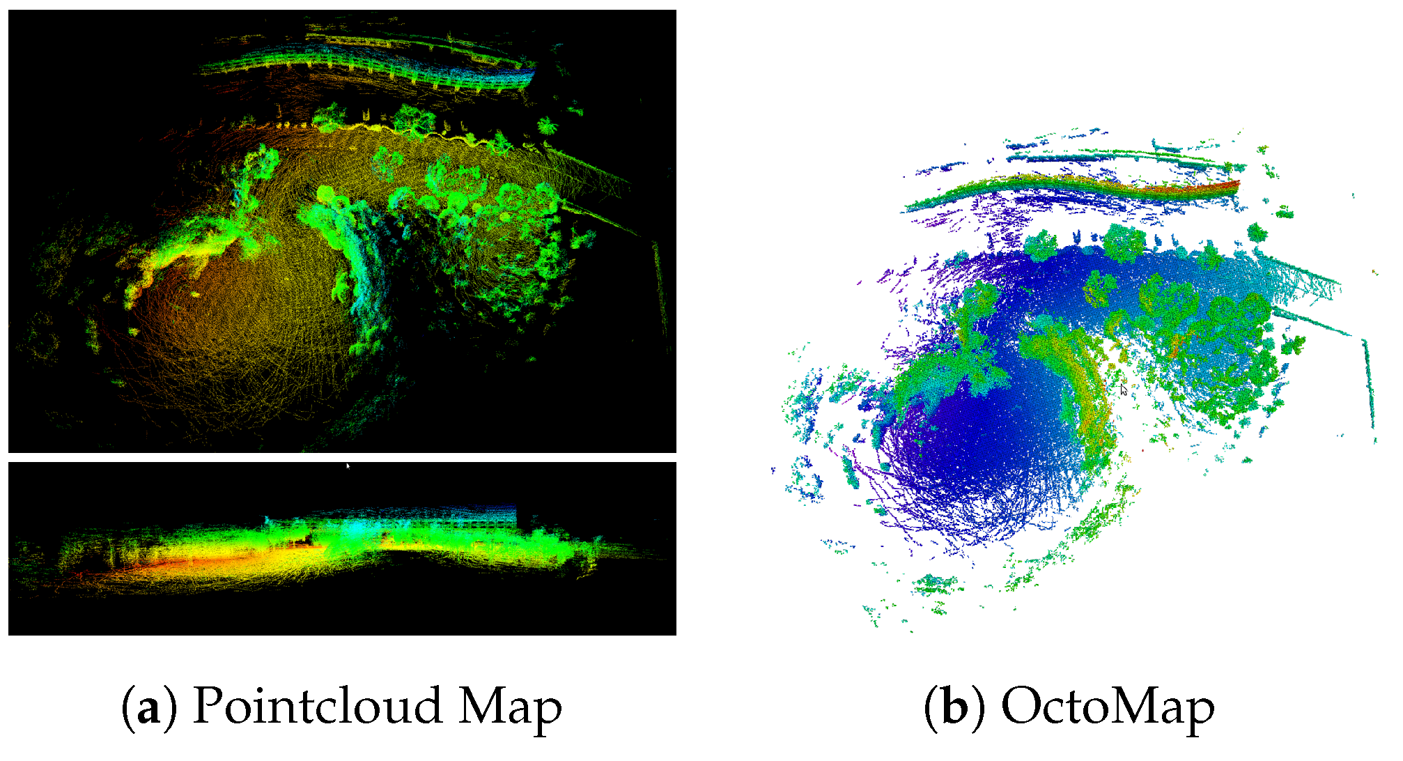
In order to obtain the curve localizability map and accessibility map of the scene, we firstly realized map building and pre-processing in the experiment using the intelligent wheelchair platform. We used a Multi-Level ICP Matching Method [25] to perform 3D SLAM based on 3D Lidar and IMU, and obtained a 3D pointcloud map as shown in Figure 7a. In order to reduce the computational complexity of following steps, we converted the pointcloud map into a OctoMap with a resolution of 0.1 m, as shown in Figure 7b.

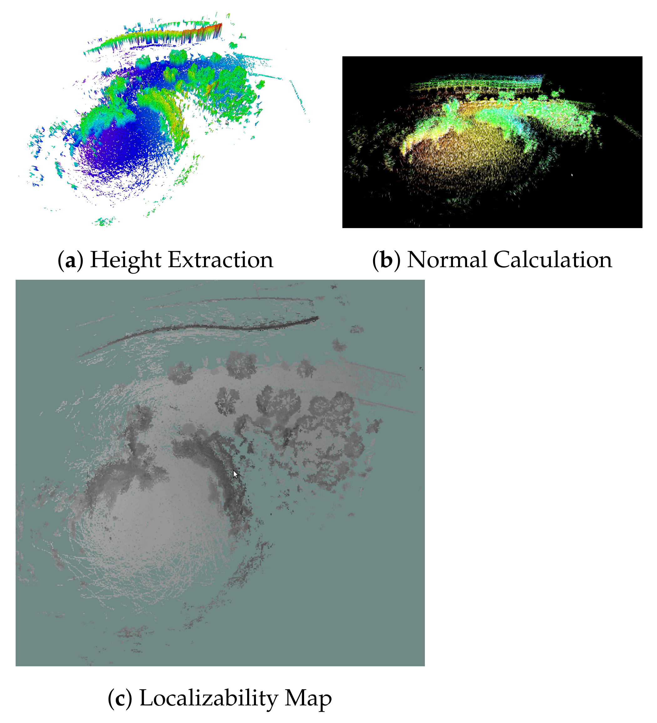
On this basis, we extracted the height and normal information of the grassland scene so as to estimate the motion curved surface of the robot and observation states of the lidar. Then the corresponding curve localizability map was calculated according to Formula (4). The results of map pre-processing and localizability map is shown in Figure 8.

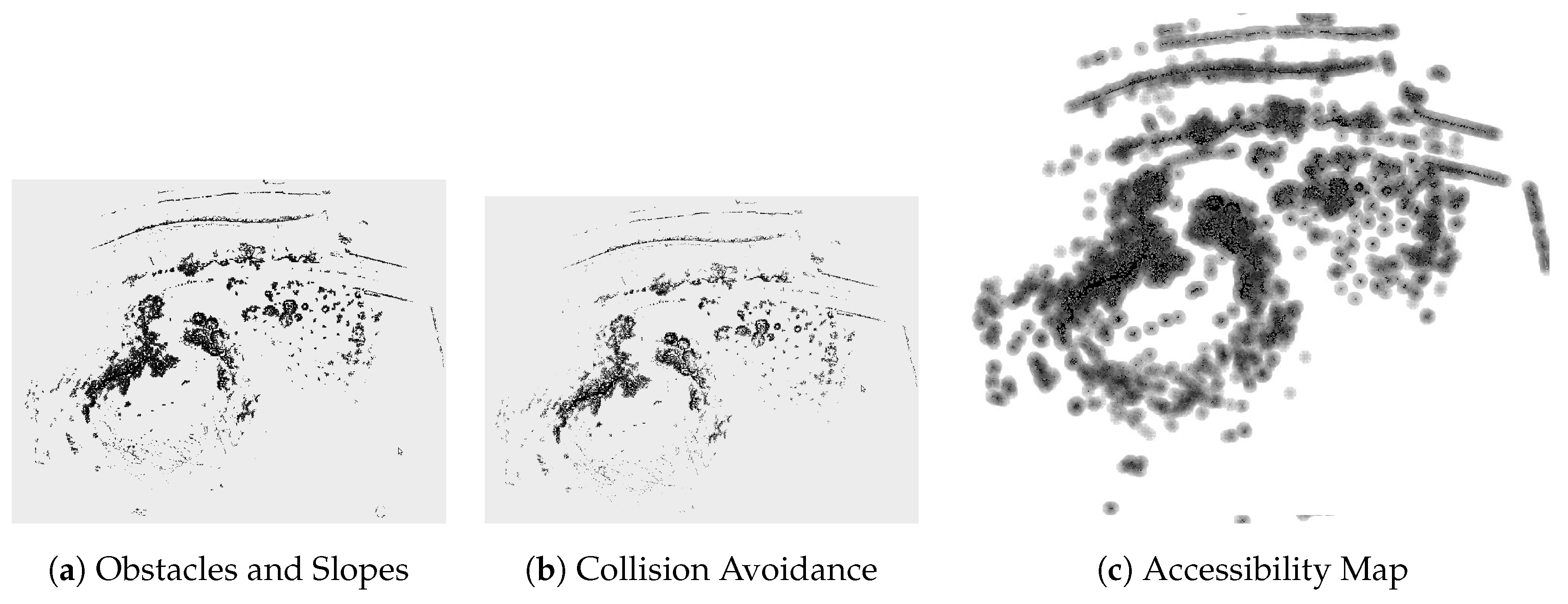
At the same time, we calculated and analyzed the map accessibility [24] for the wheelchair based on the robot model and OctoMap, taken static obstacles, slopes, and collision avoidance as the main factors, we calculated their influence on the robot accessibility in the scene and integrated these factors to generate an accessibility map. The specific process is shown in Figure 9.

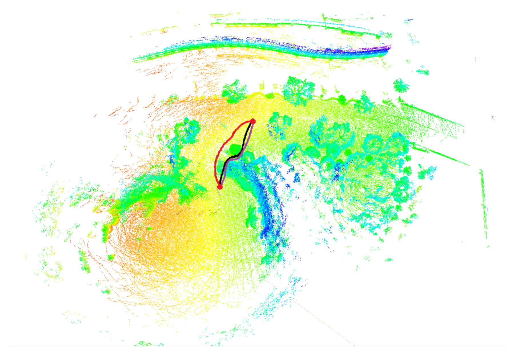
Based on the curve localizability map and accessibility map, we use the wheelchair platform to perform path planning and active localization experiments in the campus grassland scene. In order to test the effect of adding curve localizability index for robot localization, we designed three sets of path planning experiments with fixed starting and ending points. Group 1 just considers the traditional constraints of path planning, group 2 adds the entropy increment index constraint, and group 3 adds the curve localizability index constraint proposed in this paper. The three curves results are shown in Figure 10.

In order to quantitatively compare the effects of these three paths on robot localization, we use Monte Carlo particle filter algorithm to track the poses of the robot following each path. Since the true values of robot poses are difficult to obtain in this scene, we publish the localization poses in 10 Hz frequency, and record the jump values between each pose during the motion. The final result is shown in

Table 1. Results of different path planning algorithms.

	Path Planning Strategy
	Tradition Constraints	Entropy Increment	Curve Localizability
pose jumping value(m)	99.8	94.0	59.2
number of output poses	473	485	553
average of pose jumping(m)	0.211	0.194	0.107

.

It can be seen that, compared with traditional constraints and entropy increment constraint, after adding curve localizability index, although the path length is partly increased, the localization stability is significantly better than the other two paths, which verify the theoretical rationality and applicability of the curve localizability index.

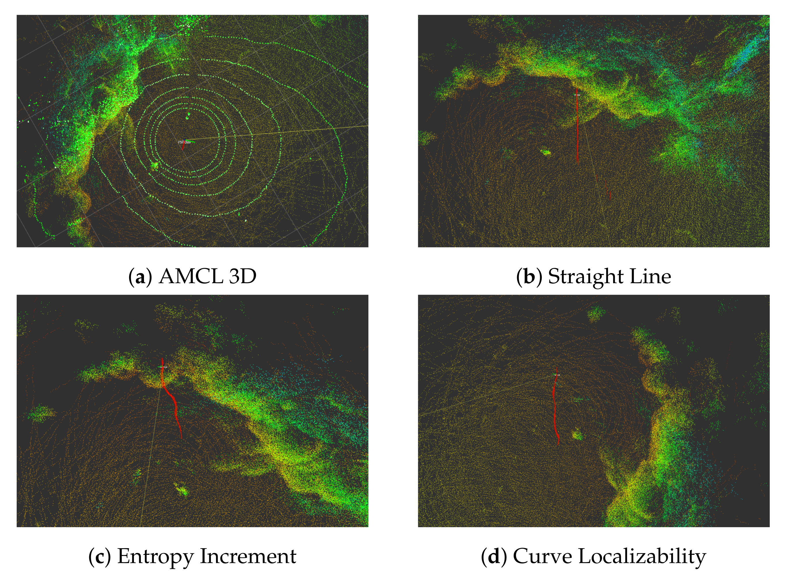
For the active localization experiments, we selected AMCL passive 3D global localization algorithm, straight-line-based active localization method, entropy-increment-based active localization method as comparisons to compare the specific performances of our algorithm on particle convergence efficiency and localization results reliability. In order to ensure the rationality of the experiment, except for AMCL strategy, both the straight-line-based and entropy-increment-based strategies used improved localization strategy in particles initialization and relocation. Setting the same start points, the robot trajectories of these four algorithms are finally shown in Figure 11.

In the four sets of experiments, the state of particles of AMCL 3D algorithm diverged with no signs of convergence within 2 min; the particles of the straight-line-based, entropy-increment-based and curve-localizability-SVM algorithm converged to the wrong poses, and then converged to the correct pose after multiple relocation, but the relocation number of our algorithm is less than other strategy. Considering the impact of the starting point on localization algorithms, we randomly selected other 7 starting points in this scene to test these algorithms. The final results are shown in

Table 2. Global localization results of different algorithms.

	AMCL 3D	Straight Line		Entropy Increment		Curve Localizability
Start Point	Time(s)	Relocation	Time(s)	Relocation	Time(s)	Relocation	Time(s)
1	Failed	7	52.2	4	41.8	4	37.1
2	7.3	0	5.1	0	5.5	0	5.3
3	52.4	4	43.5	5	37.1	2	20.2
4	Failed	5	50.8	5	44.4	4	35.7
5	Failed	Failed	Failed	Failed	Failed	7	51.9
6	8.4	0	5.0	1	16.4	1	14.3
7	8.7	0	5.3	0	5.6	0	6.0
8	Failed	3	26.1	2	19.8	2	18.6

.

From Table 2, we can see that, first of all, after several times of relocation, our algorithm can successfully converge to the correct pose, so the stability of our algorithm is higher. Secondly, compared with AMCL 3D and entropy increment method, our algorithm takes less time and and is more efficient. Because the straight-line method is just to choose the straight-line path between two points, compared with it, our algorithm has no obvious advantage in time cost, but our success rate is higher, this is very important in autonomous navigation.

5. Conclusions

This paper focuses on the active global localization of mobile robots in outdoor environments. In terms of current problems such as low calculation efficiency, poor robustness capability, and lack of active localization path planning standards of existing algorithms, this paper proposes a curve localizability index, based on OctoMap and 3D Lidar model, to estimate the relationship between lidar observation status and the robot working pose, so that we can generate an active path which is more conducive to robot localization and improve the efficiency of active localization method. We conducted comparison experiments for the proposed algorithm by actual robot platforms, and verified that our algorithm has higher computational and localization efficiency and stability under different environmental conditions through qualitative and quantitative analysis. In the future, we can consider expanding the curve localizability index to dynamic environments, or combine with other path planning and global localization strategies to satisfy specific demands of different application environments.

References

- Filliat, D. A visual bag of words method for interactive qualitative localization and mapping. In Proceedings of the IEEE International Conference on Robotics and Automation, Rome, Italy, 10–14 April 2007; pp. 3921–3926. [Google Scholar]
- Naseer, T.; Ruhnke, M.; Stachniss, C.; Spinello, L. Robust visual slam across seasons. In Proceedings of the IEEE/RSJ International Conference on Intelligent Robots & Systems, Hamburg, Germany, 28 September–2 October 2015. [Google Scholar]
- Muhammad, N.; Lacroix, S. Loop closure detection using small-sized signatures from 3d lidar data. In Proceedings of the IEEE International Symposium on Safety, Security, and Rescue Robotics, Kyoto, Japan, 1–5 November 2011; pp. 333–338. [Google Scholar]
- Magnusson, M.; Andreasson, H.; Nüchter, A.; Lilienthal, A.J. Appearance-based loop detection from 3d laser data using the normal distributions transform. In Proceedings of the IEEE International Conference on Robotics and Automation, Kobe, Japan, 12–17 May 2012; pp. 23–28. [Google Scholar]
- Dubé, R.; Dugas, D.; Stumm, E.; Nieto, J.; Siegwart, R.; Cadena, C. Segmatch: Segment based loop-closure for 3d point clouds. arXiv 2016, arXiv:1609.07720. [Google Scholar]
- Liu, J.S.; Rong, C. Sequential Monte Carlo methods for dynamic systems. J. Am. Stat. Assoc. 1998, 93, 1032–1044. [Google Scholar] [CrossRef]
- Gordon, N.J.; Salmond, D.J.; Smith, A. Novel approach to nonlinear/non-gaussian bayesian state estimation. In IEE Proceedings F (Radar and Signal Processing); IET: Washington, DC, USA, 2002; Volume 140, pp. 107–113. [Google Scholar]
- Hammersley, J.M.; Morton, K.W. Poor man’s Monte Carlo. J. R. Stat. Soc. 1954, 16, 23–38. [Google Scholar] [CrossRef]
- Dellaert, F.; Fox, D.; Burgard, W.; Thrun, S. Monte Carlo localization for mobile robots. In Proceedings of the 1999 IEEE International Conference on Robotics and Automation (Cat. No. 99CH36288C), Detroit, MI, USA, 10–15 May 1999; Volume 2, pp. 1322–1328. [Google Scholar]
- Roy, N.; Burgard, W.; Fox, D.; Thrun, S. Coastal navigation-mobile robot navigation with uncertainty in dynamic environments. In Proceedings of the 1999 IEEE International Conference on Robotics and Automation (Cat. No. 99CH36288C), Detroit, MI, USA, 10–15 May 1999; Volume 1, pp. 35–40. [Google Scholar]
- Makarenko, A.A.; Williams, S.B.; Bourgault, F.; Durrant-Whyte, H.F. An experiment in integrated exploration. In Proceedings of the IEEE/RSJ International Conference on Intelligent Robots and Systems, Lausanne, Switzerland, 30 September–4 October 2002; Volume 1, pp. 534–539. [Google Scholar]
- Porta, J.M.; Verbeek, J.J.; Krse, B.J.A. Active appearance-based robot localization using stereo vision. Auton. Robot. 2005, 18, 59–80. [Google Scholar] [CrossRef] [Green Version]
- Patric, J.; Steen, K. Active global localization for a mobile robot using multiple hypothesis tracking. IEEE Trans. Robot. Autom. 2001, 17, 748–760. [Google Scholar]
- Murtra, A.C.; Tur, J.; Sanfeliu, A. Action evaluation for mobile robot global localization in cooperative environments. Robot. Auton. Syst. 2008, 56, 807–818. [Google Scholar] [CrossRef] [Green Version]
- Hongjun, Z.; Sakane, S. Sensor planning for mobile robot localization—A hierarchical approach using a bayesian network and a particle filter. IEEE Trans. Robot. 2008, 24, 481–487. [Google Scholar]
- Yong, W.; Weidong, C.; Jingchuan, W.; Hesheng, W. Active global localization based on localizability for mobile robots. Robotica 2015, 33, 1609–1627. [Google Scholar]
- Nagarajan, P.R.; Mammen, V.; Mekala, V.; Megalai, M. A Fast And Energy Efficient Path Planning Algorithm For Offline Navigation Using Svm Classifier. Int. J. Sci. Technol. Res. 2020, 9, 2082–2086. [Google Scholar]
- Aguiar, A.S.; Santos, F.N.; Valente, A.; Petry, M.; Carlos Santos, L. Occupancy Grid and Topological Maps Extraction from Satellite Images for Path Planning in Agricultural Robots. Robotics 2020, 9, 77. [Google Scholar]
- Xu, T.; Chen, S.; Wang, D.; Wu, T.; Zhang, W. A Novel Path Planning Method for Articulated Road Roller Using Support Vector Machine and Longest Accessible Path With Course Correction. IEEE Access 2019, 7, 182784–182795. [Google Scholar]
- Charalampous, K.; Kostavelis, I.; Gasteratos, A. Thorough robot navigation based on SVM local planning. Robot. Auton. Syst. 2015, 70, 166–180. [Google Scholar] [CrossRef]
- Tennety, S.; Sarkar, S.; Hall, E.L.; Kumar, M. Support Vector Machines Based Mobile Robot Path Planning in an Unknown Environment. In Proceedings of the Dynamic Systems and Control Conference, Los Angeles, CA, USA, 12–14 October 2009; p. 48920. [Google Scholar]
- Qingyang, C.; Zhenping, S.; Daxue, L.; Yuqiang, F.; Xiaohui, L. Local path planning for an unmanned ground vehicle based on SVM. Int. J. Adv. Robot. Syst. 2012, 9, 246. [Google Scholar] [CrossRef]
- Hornung, A.; Wurm, K.M.; Bennewitz, M.; Stachniss, C.; Burgard, W. Octomap: An efficient probabilistic 3d mapping framework based on octrees. Auton. Robot. 2013, 34, 189–206. [Google Scholar] [CrossRef] [Green Version]
- Yu, X.; Wang, J.; Chen, W.; Wang, H. A map accessibility analysis algorithm for mobile robot navigation in outdoor environment. In Proceedings of the IEEE International Conference on Real-time Computing and Robotics, Irkutsk, Russia, 4–9 August 2019. [Google Scholar]
- Wang, J.; Zhao, M.; Chen, W. Mim_slam: A multi-level icp matching method for mobile robot in large-scale and sparse scenes. Appl. Sci. 2018, 8, 2432. [Google Scholar] [CrossRef] [Green Version]
Figure 1.
Framework of Curve-Localizability-Based Active Localization Algorithm.
Figure 2.
3D Omni-Direction Lidar Model.
Figure 3.
Sketch Graph of Curve Localizability.
Figure 4.
Sketch Map of Particle Initialization Improvement.
Figure 5.
Registration Result of 3D Lidar Observation Data.