
High-Order Accurate Flux-Splitting Scheme for Conservation Laws with Discontinuous Flux Function in Space

School of Mathematics and Physics, Anhui Jianzhu University, Hefei 230601, China
*
Author to whom correspondence should be addressed.
Mathematics 2021, 9(10), 1079; https://doi.org/10.3390/math9101079
Submission received: 25 March 2021
/
Revised: 27 April 2021
/
Accepted: 28 April 2021
/
Published: 11 May 2021
(This article belongs to the Special Issue Numerical Analysis and Scientific Computing)
Abstract
:A new modified Engquist–Osher-type flux-splitting scheme is proposed to approximate the scalar conservation laws with discontinuous flux function in space. The fact that the discontinuity of the fluxes in space results in the jump of the unknown function may be the reason why it is difficult to design a high-order scheme to solve this hyperbolic conservation law. In order to implement the WENO flux reconstruction, we apply the new modified Engquist–Osher-type flux to compensate for the discontinuity of fluxes in space. Together the third-order TVD Runge–Kutta time discretization, we can obtain the high-order accurate scheme, which keeps equilibrium state across the discontinuity in space, to solve the scalar conservation laws with discontinuous flux function. Some examples are given to demonstrate the good performance of the new high-order accurate scheme.
1. Introduction
We focus on the high-order accurate schemes for the conservation laws with discontinuous flux in the form
where is an unknown function, , and is the Heaviside function. Because of its interesting features and applications in traffic flows, multiple-phase flow in porus media and clarifier-thickener units model and so on, equation of this form (1) has been widely investigated in recent years [1,2,3,4,5,6,7,8].
The discontinuous flux in x results in that the Kružkov-type entropy inequalities [9] do not ensure the uniqueness of solutions to the Cauchy problem of equation of the form (1). In order to overcome this difficulty, different entropy theories have been imposed to obtain distinct choice solutions and the reader is referred to [4,5,6,7,10,11,12,13,14] for details.
Because of the discontinuity of the flux in the spatial variable x, it is very difficult to develop an efficient numerical scheme with general numerical fluxes. This implies that the interface numerical flux plays an important role in designing numerical scheme for conservation laws with discontinuous flux (1). In recent years, some efficient first-order schemes have been proposed to prove the uniqueness of weak solutions to the related model such as conservation laws (1). Based on the Godunov or EO flux, Towers [13,14] studied conservation laws with a discontinuous spatially varying coefficient or spatially varying source terms and established the convergence. Adimurthi et al. [15,16] developed the Godunov-type or DFLU numerical flux to solve scalar conservation laws with discontinuous flux. Then, Sudarshan et al. [17] extended the DFLU interface flux to two-phase multicomponent polymer flooding model and obtained a second-order scheme through the MUSCL-type reconstruction. In addition, Mishra [18] considered mixed fluxes of the convex-concave-type and concave-convex-type in (1) and defined the corresponding interface Godunov-type flux and Engquist–Osher-type flux. Karlsen and Towers [19] used the Lax–Friedrichs scheme to study conservation laws with a discontinuous space-time dependent flux. In particular, Adimurthi et al. [20] claimed that equation of the form (1) had a contractive semigroup solution in for each so-called connection-. Then, Bürger, Karlsen, Towers [21] put forward the entropy solutions of type and utilized the modified EO-type numerical scheme to prove the convergence of this type solution. Recently, Adimurthi et al. [10,22] proposed some numerical flux, including Godunov, Engquist–Osher and modified Lax–Friedrichs-type numerical fluxes to define the interface flux for -connection. In the aforementioned work, the numerical simulations show that the DFLU scheme [15,16,23] and Engquist–Osher-type scheme [21] work better than others for many models. We also see the modified Local Lax–Friedrichs flux (MLLF) [10,22], Roe-type flux [24] and application of the DFLU flux [23,25] and the references therein.
One purpose of this paper is to propose a simple and an efficient interface numerical flux, which can be easily extended to high-order schemes to approximate the conservation laws with discontinuous flux (1). With the help of the entropy solutions of type , we propose a new Engquist–Osher-type interface numerical flux, which can be written as the split form.
For the high-order accurate schemes for conservation laws with discontinuous flux (1), it is worth mentioning that Shu and his collaborators [26,27] used the Lax–Friedrichs numerical flux and the WENO reconstruction to approximate the multiclass traffic flow model on homogeneous or inhomogeneous highway. For the details of the WENO reconstruction method, we refer to [28,29,30]. Recently, Bürger, Karlsen and their collaborators [1,2,31] developed a series of second-order accurate schemes to solve the conservation laws with discontinuous flux (1). Then, borrowing the idea of flux-total variation diminishing to conservation laws with discontinuous flux introduced by Towers in [14], Bürger et al. [2] developed a nonlocal limiter algorithm and proposed a second-order flux-total variation diminishing scheme to solve the clarifier-thickener model with discontinuous flux. Adimurthi et al. made a modification of nonlocal limiter algorithm and obtained the second-order flux-TVD scheme for some interface fluxes as defined in [10]. We also refer the readers to the high-order Runge–Kutta discontinuous Galerkin scheme [32] and the semidiscrete central-upwind scheme [33].
However, so far, there are few results on the high-order schemes for (1). To the best of our knowledge, it is not easy to construct high-order schemes for (1) by using the reconstruction of the primitive variables. The reason for this may be that the discontinuity of the flux in the spatial variable x leads to the jump of the unknown function. Fortunately, the flux in (1) should satisfy the Rankine–Hugoniot condition
at the discontinuity , where represent the limits on both sides of the discontinuity , respectively. Based on this condition, we could apply the proposed Engquis–Osher type interface flux to connect two fluxes and and keep the equilibrium to capture the steady-state solution. Then, we can make use of the WENO flux reconstruction method, which introduced in [28,29,30], to develop an efficient, nonoscillatory and high-order accurate scheme for (1). This is another purpose of this paper.
The format of the paper is as follows. In Section 2, we give a new modified Engquist–Osher-type interface numerical flux, which is written into the flux-splitting form. In Section 3, we propose three high-order schemes for (1) by using the modified Engquist–Osher type interface flux or DFLU flux and the WENO reconstruction. In Section 4, some numerical examples are presented. Finally, we make a discussion about three high-order accurate schemes.
2. The Modified Engquist–Osher-Type Interface Numerical Flux
Based on the -connection [20] and the entropy solutions of type [21], we suppose that the flux in (1) satisfies:
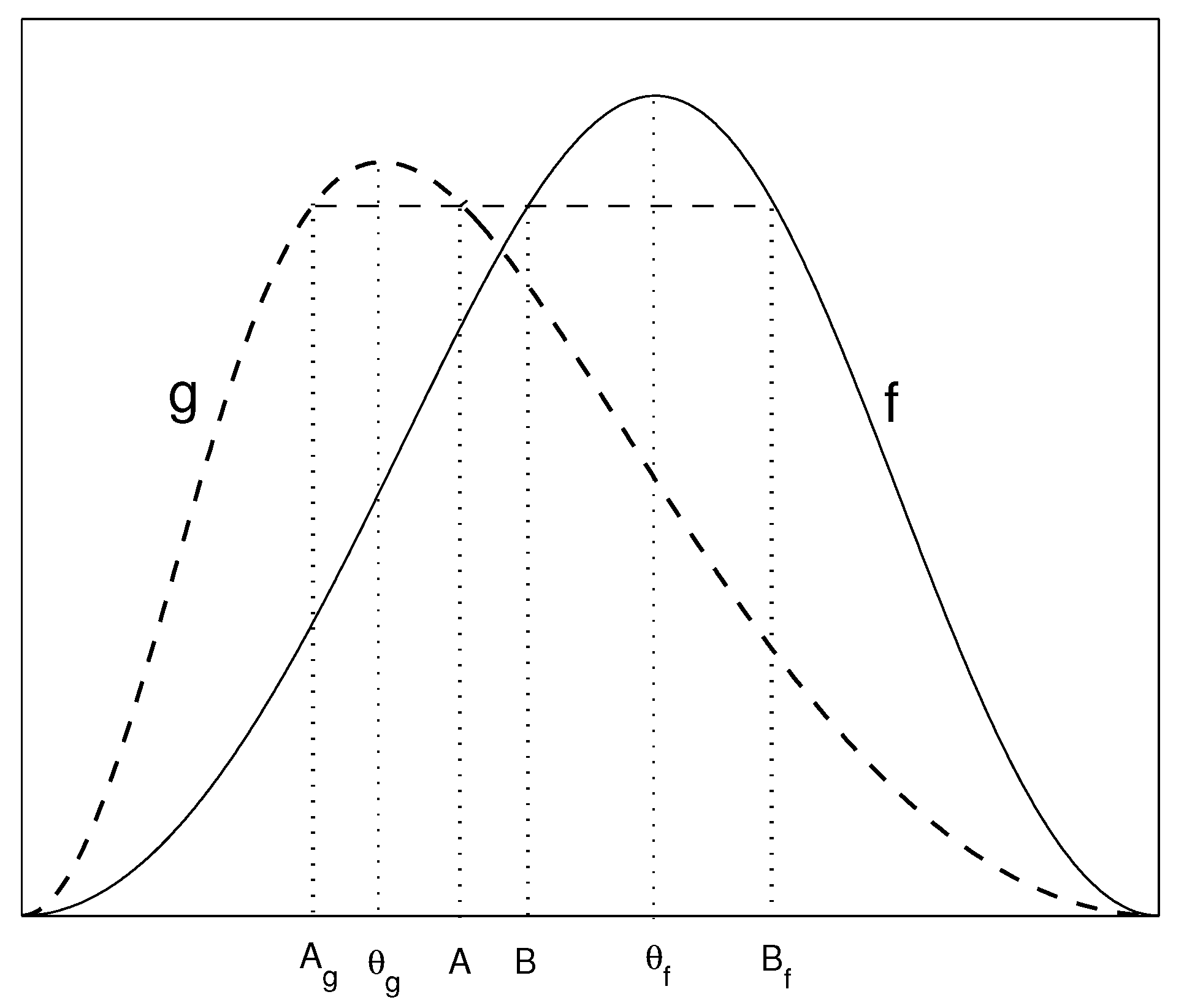
(A1), for , f has a single maximum at and g has a single maximum at . The function f (or g) is strictly increasing on (or ) and strictly decreasing on (or ).
(A2) both f and g are genuinely nonlinear in the sense that f and g are not linear on any nondegenerate interval.
(A3) there exists at most one point such that .
For convenience, set
The corresponding Engquist–Osher numerical flux is
which can be written as the flux-splitting form
where
As stated above, the interface numerical flux plays a key role in designing the numerical methods for (1). So, we modify the Engquist–Osher-type interface numerical flux to approximate (1) with -connection.
Under the assumptions –, without the loss of generality, the graphs of functions , and the connection are shown in Figure 1. Obviously, there exist such that they satisfy , and . With the following definitions
We can generalize the Engquist–Osher interface numerical flux (4) and (5) in the form
to capture the entropy solutions of type , where
By the discussion case by case, we can obtain that the modified Engquist–Osher interface numerical flux (7) and (8) is equivalent to the interface flux introduced by Bürger, Karlsen, Towers in [21]. Besides this, the new interface flux-splitting form (7) and (8) is simple and can be extended to the high-order approximation by using the WENO reconstruction, see Section 3.
Next, we consider the important properties of the flux .
Lemma 1.
Based on the flux function , we have:
- (1)
- is nondecreasing function in its first variable, nonincreasing function in its second variable, and Lipschitz continuous on both two arguments.
- (2)
- is not consistent, but , , and .
Proof.
For any , , we have
where
Thus, the statement (1) is true.
The proof of assertion (2) is trivial. So, we proof the Lemma. □
Now, we consider the initial value problem (1) with the initial data
where and are some constants. For simplicity, we use a uniform space and time grid with space size and time step to approximate solution of (1). Define the space grid points and . Let , for . Set and for . Based on (4)–(9), we construct the numerical scheme for (1) as follows
where
3. High-Order Accurate Schemes for Conservation Laws (1)
In this section, we present two types of high-order accurate schemes to solve (1) by using the idea of WENO reconstruction.
3.1. High-Order WENO Scheme Based on the Modified Interface Engquist–Osher-Type Flux
Although the unknown function u is jump across the discontinuity for (1), the Rankine–Hugoniot condition (2) implies that we could add the interface flux (7) to connect the two fluxes. So, we can take advantage of the idea of WENO reconstruction of fluxes to construct high-order scheme, which is of the form
in which is the numerical flux to be given below.
To ensure the numerical stability and correct upwind biasing, we utilize the Engquist–Osher-type flux-splitting form (4) and (7) to construct the numerical flux as follows
Here, we can adopt the fifth-order WENO reconstruction method [28,29,30] to construct and . The procedure includes the following two steps.
Step 1. Away from the discontinuity .
We give three third-order accurate numerical fluxes for the case as follows
In this case, we describe the smoothness indicators as
and give the linear weights
Then, we use the nonlinear weights
to define
Here, is a small constant and taken as to prevent the denominator to be zero. Performing the mirror symmetric with respect to , we can obtain the reconstruction procedure for the flux . We omit the details and refer to [28,29,30] on this issue.
Step 2. Near the discontinuity .
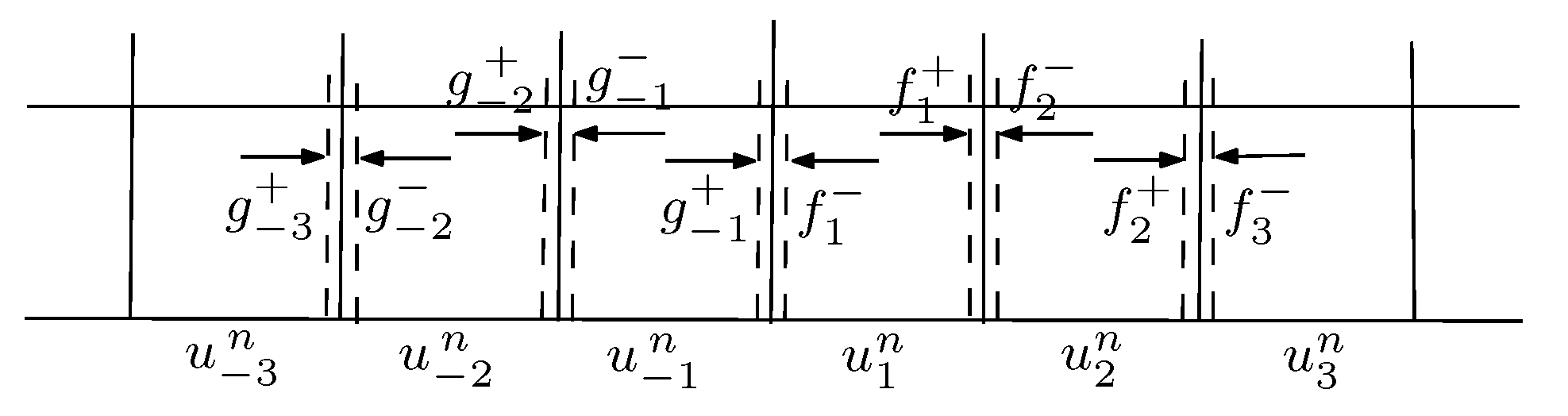
Since the flux changes when passing the discontinuity , it is not easy for us to reconstruct the and for . In order to overcome this difficulty, we could replace and with this and respectively, as shown in Figure 2. So we set
to construct for and set
to construct for as the procedure in Section 3.1. Similarly, we also reconstruct and for .
3.2. High-Order WENO Schemes Based on the Reconstructions of the Unknown Functions
In this subsection, we adopt the so-called DFLU numerical flux introduced in [15,16] and the WENO reconstruction method to present the other two high-order WENO schemes.
For the fluxes , and the connection shown in Figure 1, the DFLU numerical fluxes can be defined as the following form
Then, the numerical flux in (14) can be written as
where are prescribed as follows.
We directly utilize the unknown functions () to construct and for . Similar to the procedure in Section 3.1, we set
and use five variables , to reconstruct and for and at the same time set
to reconstruct and for . Thus combining (14), (24) and (21) gives the high-order accurate WENO scheme for (1), denoted by DFLU-WENO5.
It is important to capture steady-state solution and prevent spurious oscillations near the discontinuity for (1). Then, we adopt the idea of the well-balanced method [35,36,37] to construct . Suppose be a pair of well-balanced solution or steady-state solution to the initial data problem (1) and (10). Different from the above DFLU-WENO5 method, we use
satisfying and , to construct and for and
satisfying to construct and for . Once again, we implement (21) to obtain the high-order scheme with the well-balanced method or preserving the steady-state solution, which is termed as DFLU-WENO5B.
4. Numerical Examples
To demonstrate the efficiency of our methods, we here present some numerical results of the new first-order MEO scheme, DFLU scheme consisting of numerical fluxes (22) and (23), and three high-order WENO schemes which are described in Section 2 and Section 3 for comparison. For convenience, the first-order MEO scheme and the first-order DFLU scheme are termed as MEO-1 and DFLU-1, respectively.
Example 1.
We consider the case for traffic flow, where the fluxes can be taken asandin (1). We take the initial data as follows
For this case, the connect-can be taken asand the steady-state solution is. The numerical parameterand the compute time. In this case, the exact Riemann solution can be given in follows
The -errors computed by the above five methods MEO-1, DFLU-1, MEO-WENO5, DFLU-WENO5, and DFLU-WENO5B are given in the Table 1. Although -errors of the MEO-1 scheme are slightly larger than those of the DFLU-1 scheme, they have the same numerical results. However, MEO-WENO5 scheme has smaller -errors than DFLU-WENO5 starting with and , which indicates that the MEO-WENO5 has better performance than the DFLU-WENO5. In addition, we can observe that the DFLU-WENO5B scheme has smaller numerical -errors than the MEO-WENO5 and DFLU-WENO5 schemes.
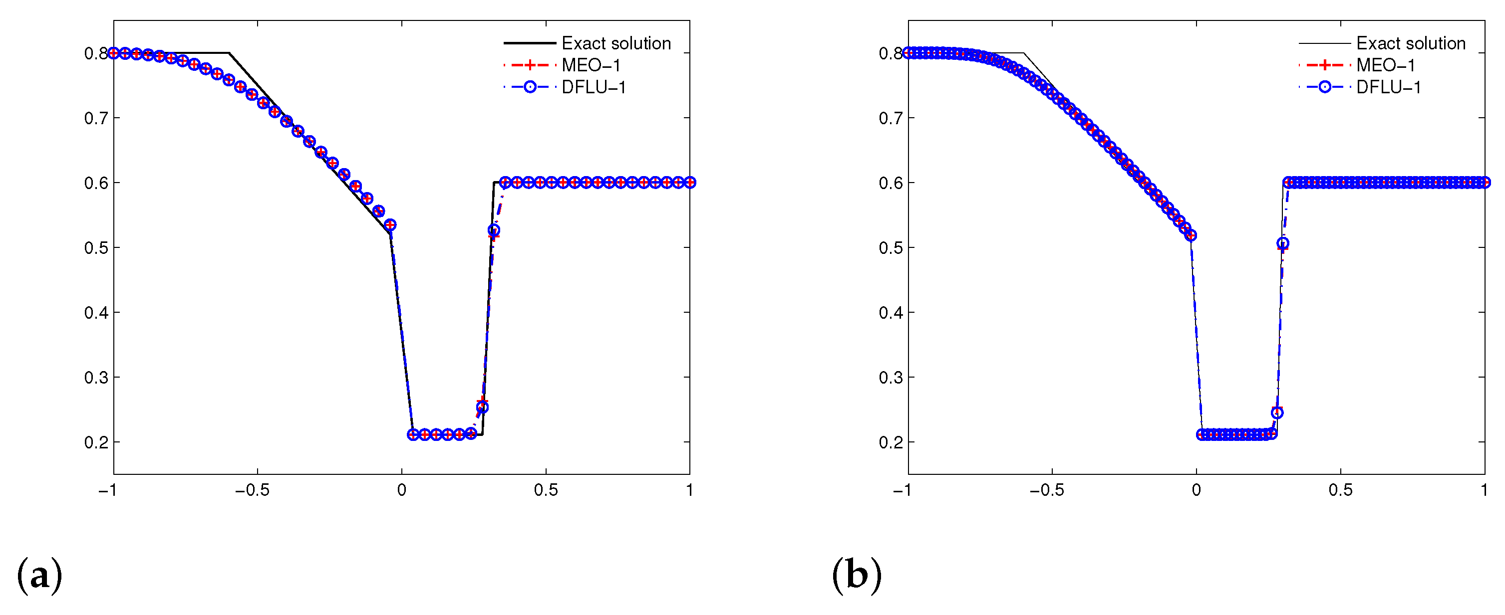
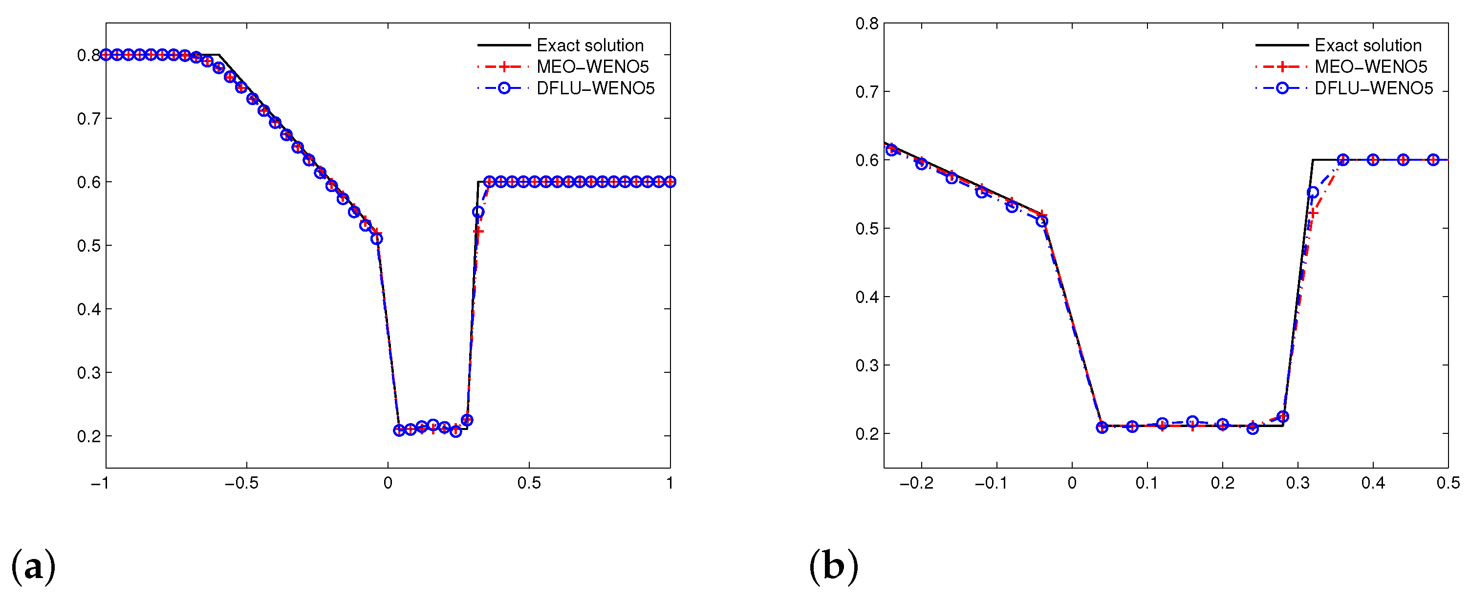
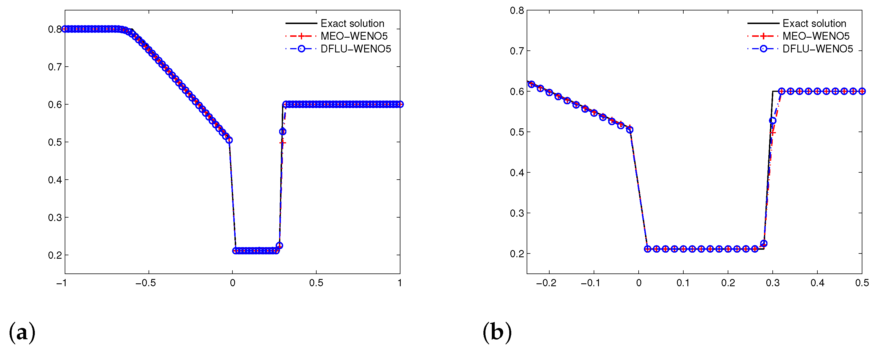
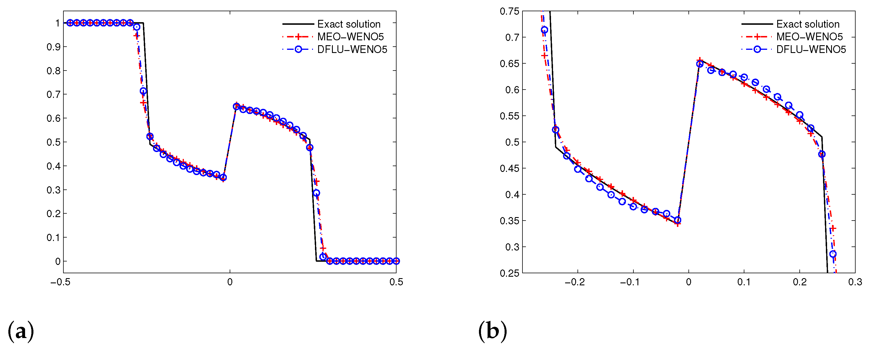
To further analyze these schemes, we present the numerical solutions with space sizes and , where the solid line represents exact solutions in the following figures. Figure 3 shows that the MEO-1 and the DFLU-1 perform equally well and they can capture the solution to initial value problem (1) and (29). Figure 4 illustrates that the MEO-WENO5 works better than the DFLU-WENO5 near the discontinuity . Moreover, we observe that the numerical solution computed by MEO-WENO5 is in better agreement with the exact solution than the DFLU-WENO5. The main reason for this situation is that the DFLU-WENO5 scheme produces spurious oscillations behind the shock and the discrepancy between the numerical solution and the exact solution can be observed near the discontinuity . As the mesh is refined, the above oscillations disappears but the discrepancy still exists, as shown in Figure 5.
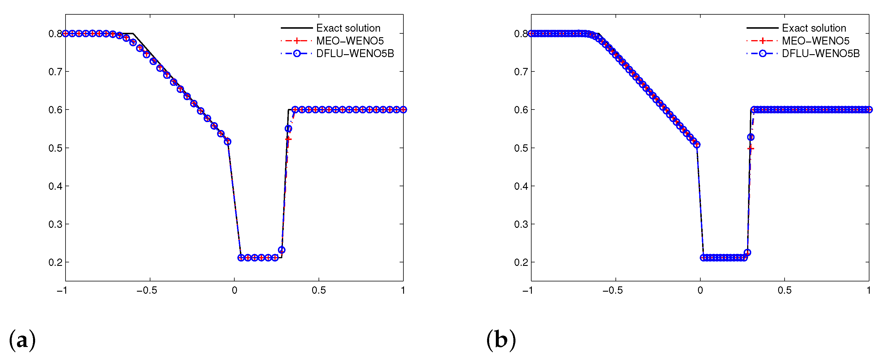
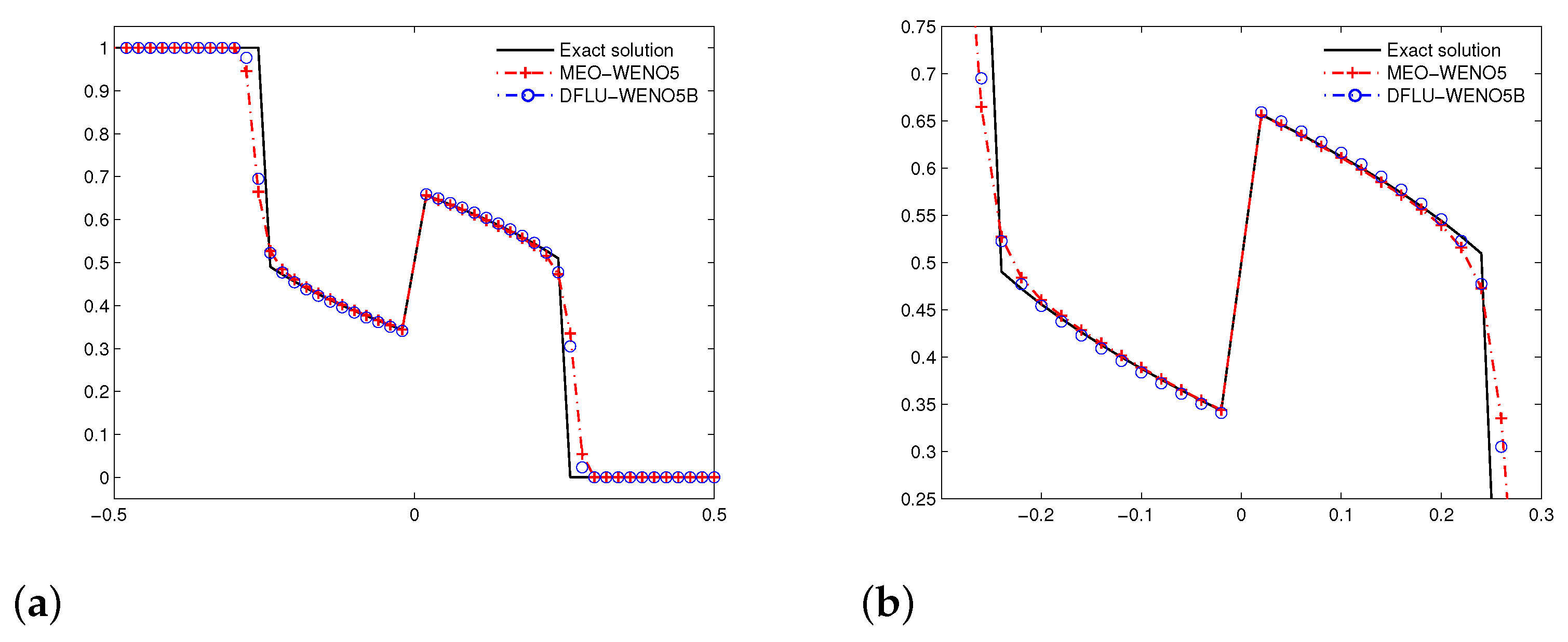
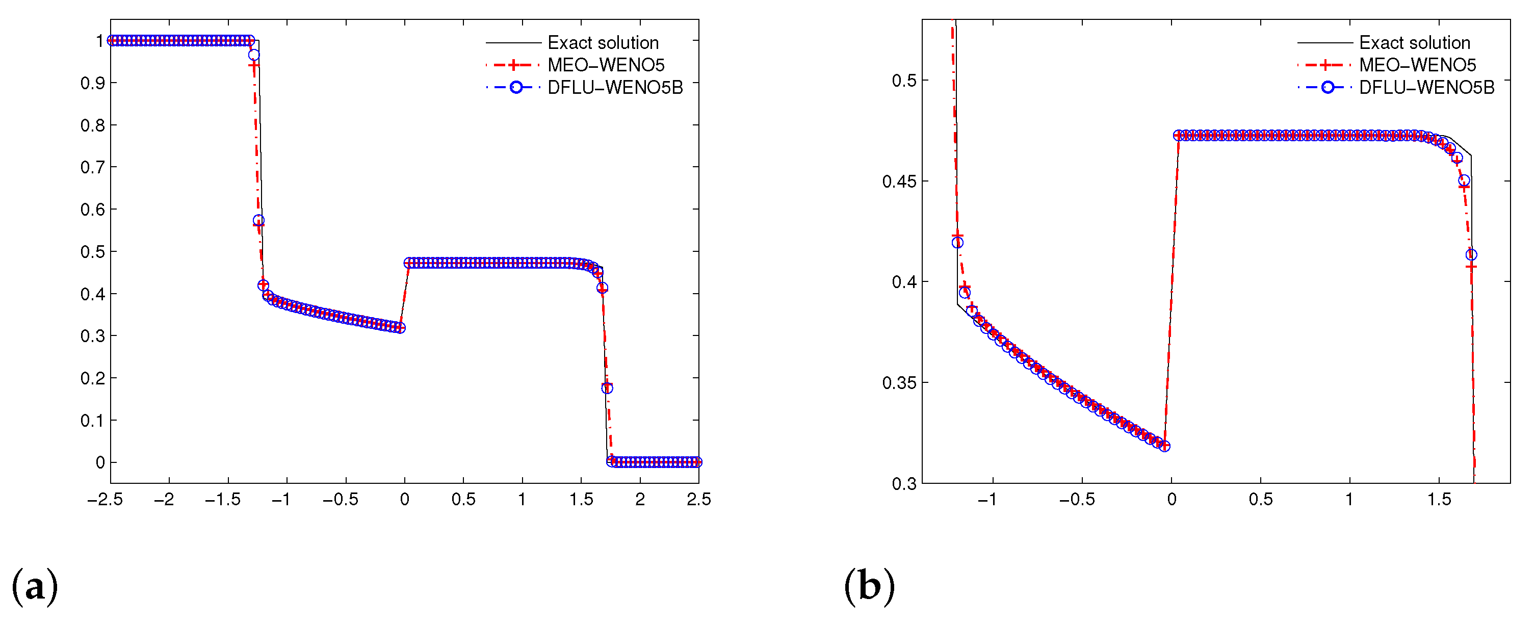
We now solve the initial value problem (1) and (29) with space sizes and by MEO-WENO5 and DFLU-WENO5B, respectively. The numerical solutions are shown in Figure 6, from which a good agreement with the exact solution presented by both two schemes is observed. Moreover, the DFLU-WENO5B does not introduce the oscillation behind the shock, but the discrepancy mentioned above on the left of the discontinuity still exists.
Example 2.
To investigate the above two aspects, we take the fluxesandcoming from [21] and the initial conditions for and for . Set and the connection-. So we obtain the steady-state solution . For the fluxes and in this case, there exist and such that they satisfy
may see Figure 1. Now, we present the exact Riemann solution as
which includes a contact discontinuity connecting two states and 1 and another contact discontinuity connecting two states 0 and .
We compute the solution up to and present the numerical -errors of the above five schemes in Table 2, which shows that the -error of MEO-1 is slight smaller than that of DFLU-1, meanwhile both DFLU-WENO5 and DFLU-WENO5B schemes have smaller numerical error than the MEO-WENO5 scheme. Next, we further analyze the numerical solution to explore this situation.
We first compute the initial value problem by the MEO-1 and DFLU-1 schemes with space sizes and , respectively. It is easy to see that they have similar behavior, see Figure 7.
Now we present the numerical solutions by the three high-order accurate schemes with space size , as illustrated in Figure 8. The solution of two rarefactive waves on both sides of the discontinuity has been well approximated by the MEO-WENO5 scheme. However, the numerical solutions computed by the DFLU-WENO5 and DFLU-WENO5B are slightly different from the exact solution. Especially, the DFLU-WENO5 scheme gives rise to more oscillations.
Finally, the numerical solutions are presented in Figure 9 and Figure 10 as mesh refinement with space size . Figure 9 shows that the DFLU-WENO5 introduces the spurious oscillations on both sides of , but Figure 10 illustrates that the oscillation disappears for the DFLU-WENO5B. In addition, both the DFLU-WENO5 and DFLU-WENO5B perform better resolution of contact discontinuity away from the discontinuity than the MEO-WENO5. This may be the reason why the -errors performed by the DFLU-WENO5 and DFLU-WENO5B are smaller than those performed by the MEO-WENO5.
Example 3
([15]). Considering the two-phase incompressible flow in a porous medium with a rock type changing at . The flux functions and have the following form
Under the following data
Two fluxes and are represented in Figure 1. The initial data is for and for with the connection . The difference from the previous Example 2 is that the contact discontinuity on the left of the stationary discontinuity is replaced by the constant state B and a composite wave consisting of a rarefaction wave and a contact discontinuity. We take the numerical parameter and compute the solution up to time .
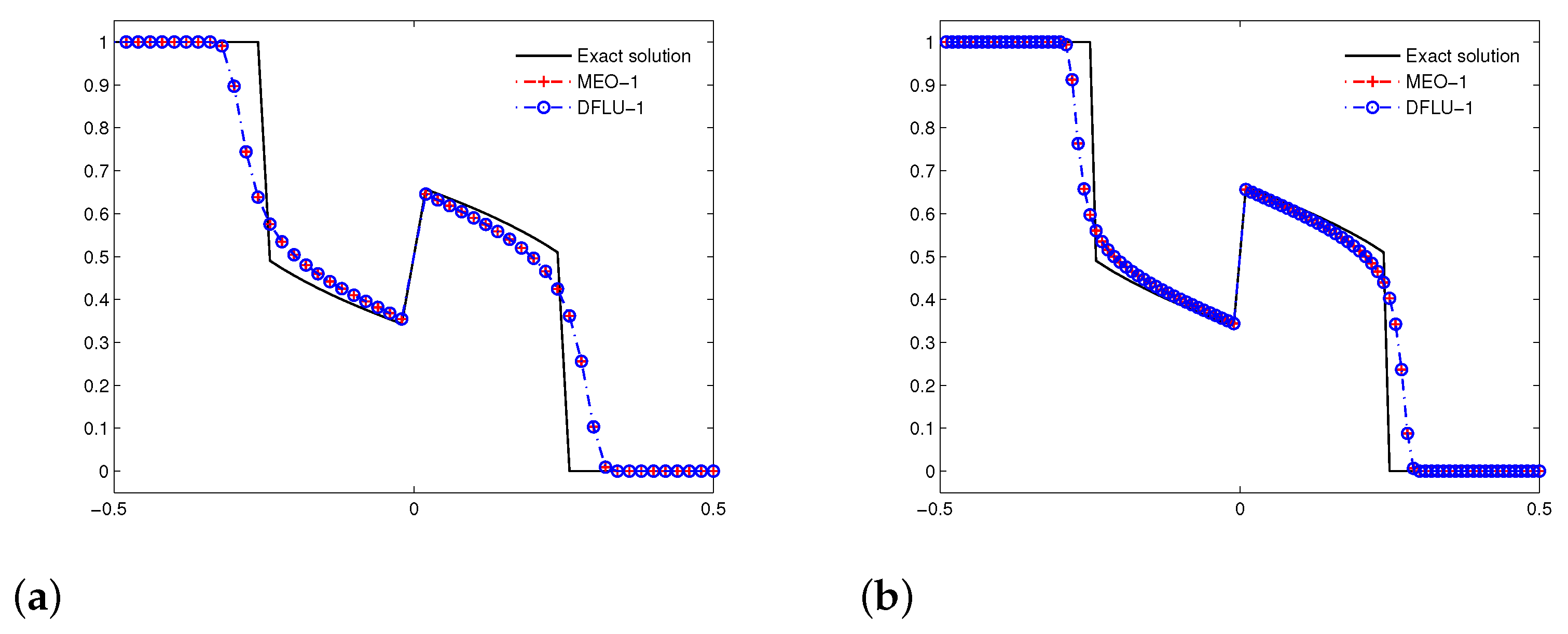
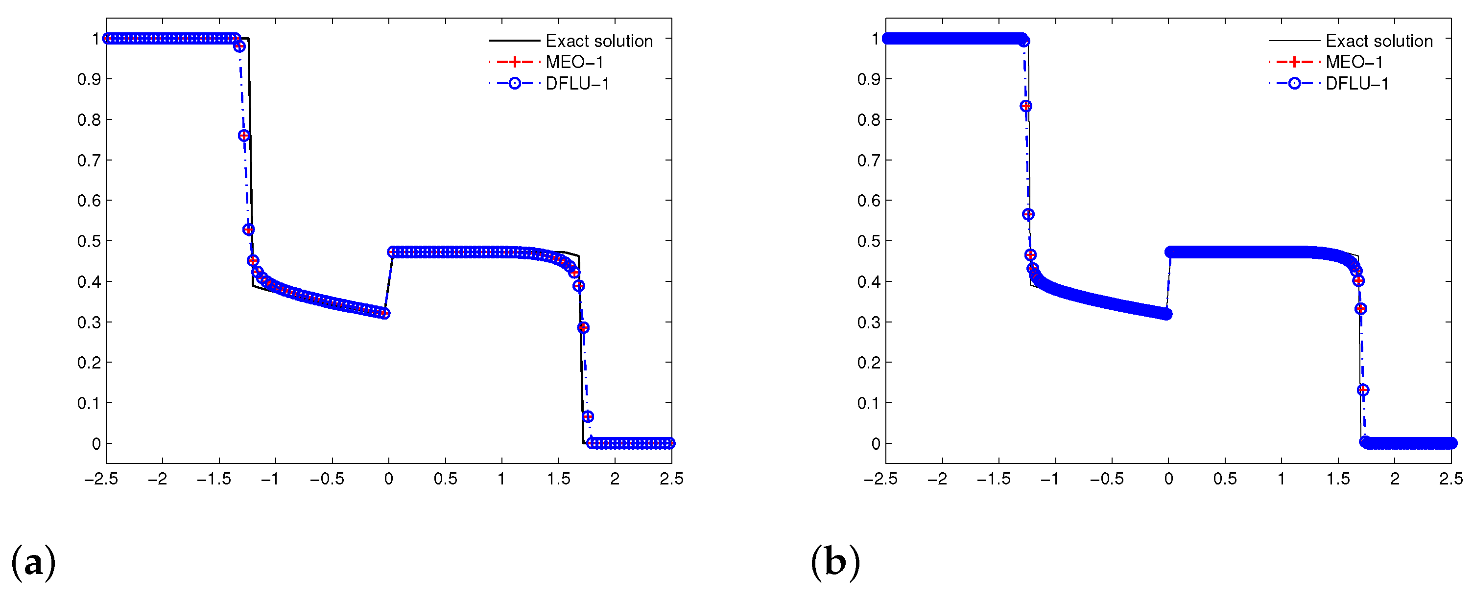
We first make use of the MEO-1 and DFLU-1 schemes to compute this problem with and , respectively. The numerical solutions are illustrated in Figure 11. It is apparent that the MEO-1 scheme performs as well as the DFLU-1 scheme.
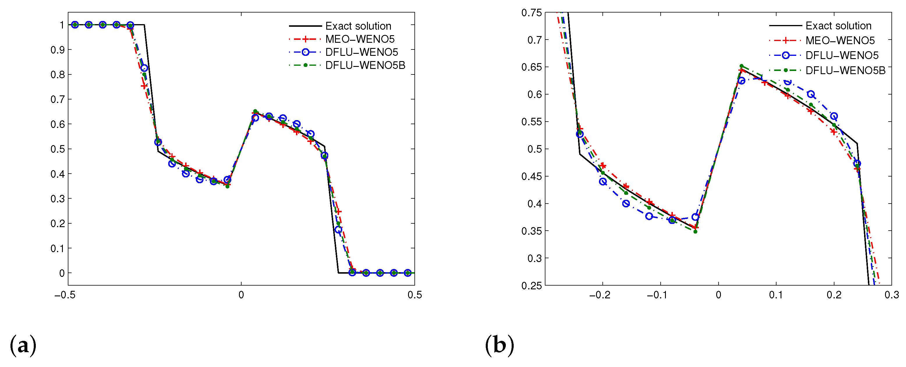
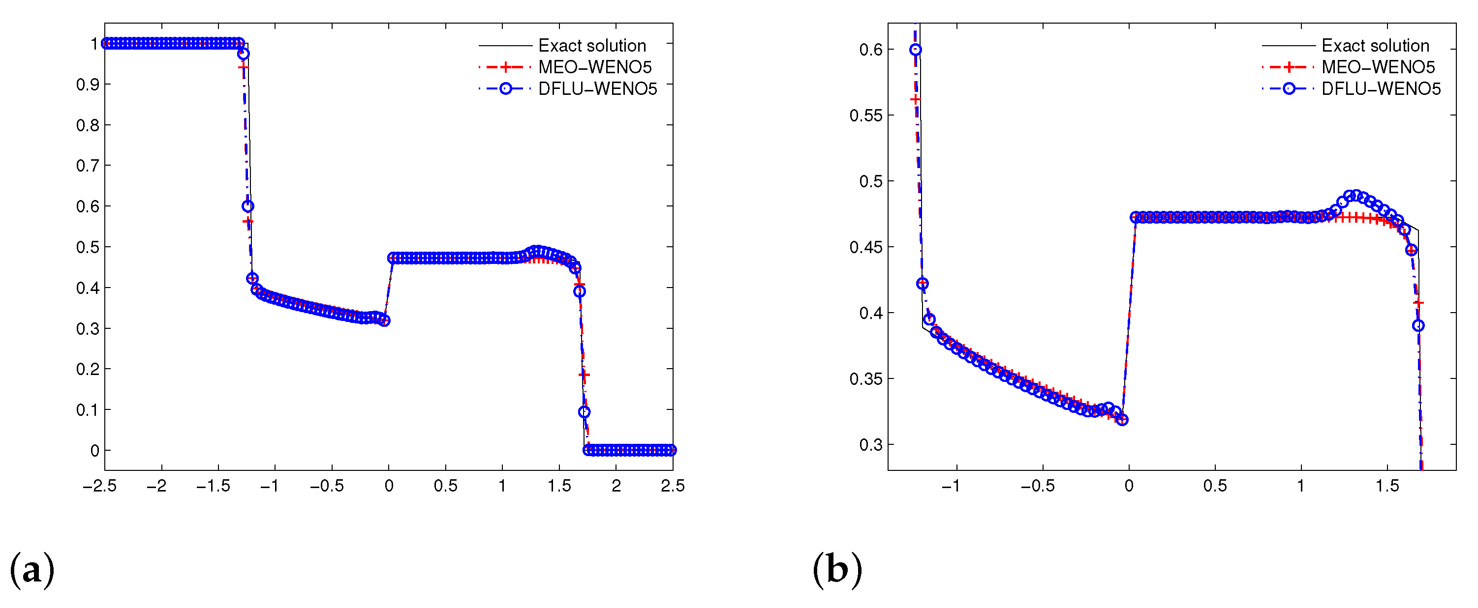
Now, we utilize three high-order schemes to compute this problem with space size and present the numerical solutions. In Figure 12, we see that the DFLU-WENO5 scheme gives rise to spurious oscillations and has slight deviation from the exact solution on the left of . We easily observe from Figure 13 that both MEO-WENO5 and DFLU-WENO5B schemes are in good agreement with the exact solution. However, the discrepancy between the numerical solution computed by the DFLU-WENO5B scheme and the exact solution can still be found in the rarefaction wave region on the left of .
5. Conclusions
In this paper, we propose the new first-order modified Engquist–Osher-type scheme (MEO), which performs as well as the DFLU scheme [15,16,25] and the modified EO-scheme [21]. The new modified EO-type interface flux could be written as the split form (7) and (8), which contributes to stability of the scheme and could be taken as a building block for constructing high-order scheme. As mentioned before, the flux in (1) should satisfy the Rankine–Hugoniot condition (2), thus the interface numerical flux (7) could be used as a bridge connecting two flux functions and . Therefore, we bring this result to the WENO reconstruction of fluxes and achieve the high-order accurate scheme (MEO-WENO5). Based on the well-balanced method or the steady-state solution, we apply the WENO method to construct another high-order accurate scheme (DFLU-WENO5B). In comparison with the DFLU-WENO5 and DFLU-WENO5B, the MEO-WENO5 makes use of the reconstruction of fluxes, instead of the reconstruction of unknown functions, which shows its conservative to the discontinuity and still keeps nonoscillatory, especially in areas near the discontinuity . However, the scheme proposed in this manuscript could not be directly generalized to approximate the system of hyperbolic balance laws involving the discontinuous flux in space, since it is difficult to define the approximate interface flux. However, by virtue of some special methods, such as the idea of discontinuous flux, we could solve some special system of hyperbolic conservation laws involving the discontinuous flux.
Author Contributions
Investigation, T.X.; methodology, G.W.; software, T.X. and S.Z. All authors have read and agreed to the published version of the manuscript.
Funding
This work was supported by the Anhui Provincial Natural Science Foundation under grant 2008085QA12; the University Natural Science Research Project of Anhui Province under grants KJ2019A0782, KJ2019A0786, and the Key Laboratory of Architectural Acoustic Environment of Anhui Higher Education Institutes.
Institutional Review Board Statement
Not applicable.
Informed Consent Statement
Not applicable.
Data Availability Statement
Not applicable.
Conflicts of Interest
The authors declare no conflict of interest.
References
- Bürger, R.; Garcia, A.; Karlsen, K.H.; Towers, J.D. A family of numerical schemes for kinematic flows with discontinuous flux. J. Eng. Math. 2008, 60, 387–425. [Google Scholar] [CrossRef]
- Bürger, R.; Karlsen, K.H.; Torres, H.; Towers, J.D. Second-order schemes for conservation laws with discontinuous flux modelling clarifier-thickener units. Numer. Math. 2010, 116, 579–617. [Google Scholar] [CrossRef] [Green Version]
- Bürger, R.; Karlsen, K.H.; Risebro, N.H.; Towers, J.D. Well-posedness in BVt and convergence of a difference scheme for continuous sedimentation in ideal clarifier-thickener units. Numer. Math. 2014, 97, 25–65. [Google Scholar] [CrossRef] [Green Version]
- Diehl, S. On scalar conservation laws with point source and discontinuous flux functions. SIAM J. Math. Anal. 1995, 26, 1425–1451. [Google Scholar] [CrossRef] [Green Version]
- Diehl, S. A conservation laws with point source and discontinuous flux function modelling continuous sedimentation. SIAM J. Math. Anal. 1996, 56, 388–419. [Google Scholar] [CrossRef] [Green Version]
- Gimse, T.; Risebro, N.H. Riemann problem with a discontinuous flux fuction. In Proceedings of the Third International Conference on Hyperbolic Problem, Theory, Numerical Methods and Applications, Uppsala, Sweden, 11–15 June 1991; pp. 488–502. [Google Scholar]
- Gimse, T.; Risebro, N.H. Solutions of the Cauchy problem for a conservation law with discontinuous flux functions. SIAM J. Appl. Math. 1992, 56, 635–648. [Google Scholar] [CrossRef]
- Mochen, S. An analysis for the traffic on highways with changing surface conditions. Math. Model 1987, 9, 1–11. [Google Scholar] [CrossRef] [Green Version]
- Kružkov, S.N. First order quasilinear equations with several independent variables. Math. USSR-Sb. 1970, 10, 217–243. [Google Scholar]
- Adimurthi; Dutta, R.; Veerappa Gowda, G.D.; Jaffré, J. Monotone (A,B) entropy stable numerical scheme for scalar conservation laws with discontinuous flux. ESAIM Math. Model. Numer. Anal. 2014, 48, 1725–1755. [Google Scholar] [CrossRef] [Green Version]
- Klingenber, C.; Risebro, N.H. Convex conservation laws with discontinuous coeffients. existence, uniqueness and asymptotic behavior. Commun. Part. Differ. Equ. 1995, 20, 1959–1990. [Google Scholar] [CrossRef]
- Seaid, M. Stable numerical methods for conservation laws with discontinuous flux function. Appl. Math. Comput. 2006, 175, 383–400. [Google Scholar] [CrossRef]
- Towers, J.D. Convergence of a difference scheme for conservation laws with a discontinuous flux. SIAM J. Numer. Anal. 2000, 38, 681–698. [Google Scholar] [CrossRef] [Green Version]
- Towers, J.D. A difference scheme for conservation laws with a discontinuous flux: The nonconvex case. SIAM J. Numer. Anal. 2001, 39, 1197–1218. [Google Scholar] [CrossRef] [Green Version]
- Adimurthi; Jaffré, J.; Veerappa Gowda, G.D. Godunov-Type methods for conservation law with discontinuous flux. SIAM J. Numer. Anal. 2004, 42, 179–208. [Google Scholar]
- Adimurthi; Jaffré, J.; Veerappa Gowda, G.D. The DFLU flux for systems of conservation laws. J. Comput. Appl. Math. 2013, 247, 102–123. [Google Scholar] [CrossRef]
- Sudarshan, K.K.; Praveen, C.; Veerappa Gowda, G.D. A finite volume method for a two-phase multicomponent polymer flooding. J. Comput. Phys. 2014, 275, 667–695. [Google Scholar]
- Mishra, S. Convergence of upwind finite difference schemes for a scalar conservation law with indefinite discontinuities in the flux function. SIAM J. Numer. Anal. 2005, 43, 559–577. [Google Scholar] [CrossRef]
- Karlsen, K.H.; Towers, J.D. Convergence of the Lax-Friedrichs scheme and stability for conservation laws with a discontinuous space-time dependent flux. Chin. Ann. Math. Ser. B 2004, 25, 287–318. [Google Scholar] [CrossRef]
- Adimurthi; Mishra,, S.; Veerappa Gowda, G.D. Optimal entropy solutions for conservation laws with discontinuous flux functions. J. Hyperbolic Differ. Equ. 2005, 2, 783–837. [Google Scholar] [CrossRef]
- Bürger, R.; Karlsen, K.H.; Towers, J.D. An Engquist-Osher-type scheme for conservation laws with discontinuous flux adapted to flux connections. SIAM J. Numer. Anal. 2009, 47, 1684–1712. [Google Scholar] [CrossRef] [Green Version]
- Adimurthi; Sudarshan, K.K.; Veerappa Gowda, G.D. Second order scheme for scalar conservation laws with discontinuous flux. Appl. Numer. Math. 2014, 80, 46–64. [Google Scholar] [CrossRef]
- The Godunov scheme for scalar conservation laws with discontinuous bell-shaped flux functions. Appl. Math. Lett. 2012, 64, 1844–1848.
- Wang, G.; Hu, Y. The Roe-type interface flux for conservation laws with discontinuous flux function. Appl. Math. Lett. 2018, 75, 68–73. [Google Scholar] [CrossRef]
- Bürger, R.; Kumar, S.; Kenettinkara, S.K.; Ricardo, R.B. Discontinuous approximation of viscous two-phase flow in heterogeneous porous media. J. Comput. Phys. 2016, 321, 126–150. [Google Scholar] [CrossRef]
- Zhang, M.; Shu, C.-W.; Wong, G.C.K.; Wong, S.C. A weighted essentially non-oscillatory numerical scheme for a multi-class Lighthill-Whitham-Richards traffic flow model. J. Comput. Phys. 2003, 191, 639–659. [Google Scholar] [CrossRef]
- Zhang, P.; Wong, S.C.; Shu, C.-W. A weighted essentially non-oscillatory numerical scheme for a multi-class traffic flow model on an inhomogeneous highway. J. Comput. Phys. 2006, 212, 739–756. [Google Scholar] [CrossRef]
- Shu, C.-W. Essentially non-oscillatory and weighted essentially non-oscillatory schemes for hyperbolic conservation laws. Advanced Numerical Approximation of Nonlinear Hyperbolic Equations. In Lecture Notes in Mathematics; Quarteroni, A., Ed.; Springer: Berlin/Heidelberg, Germany, 1998; Volume 1697, pp. 325–432. [Google Scholar]
- Shu, C.-W. High order weighted essentially nonoscillatory schemes for convection dominated problems. SIAM Rev. 2009, 51, 82–126. [Google Scholar] [CrossRef] [Green Version]
- Jiang, G.; Shu, C.-W. Efficient implementation of weighted ENO schemes. J. Comput. Phys. 1996, 126, 202–228. [Google Scholar] [CrossRef] [Green Version]
- Berresa, S.; Bürger, R.; Karlsen, K.H. Central schemes and systems of conservation laws with discontinuous coefficients modeling gravity separation of polydisperse suspensions. J. Comput. Appl. Math. 2004, 164, 53–80. [Google Scholar]
- Qiao, D.-L.; Zhang, P.; Lin, Z.-Y.; Wong, S.C.; Choid, K. A Runge-Kutta discontinuous Galerkin scheme for hyperbolic conservation laws with discontinuous fluxes. Appl. Math. Comput. 2017, 292, 309–319. [Google Scholar] [CrossRef] [Green Version]
- Wang, G.; Ge, C. Semidiscrete central-upwind scheme for conservation laws with a discontinuous flux function in space. Appl. Math. Comput. 2011, 217, 7065–7073. [Google Scholar] [CrossRef]
- Gottlieb, S.; Shu, C.-W. Total variation diminishing Runge-Kutta schemes. Math. Comput. 1998, 67, 73–85. [Google Scholar] [CrossRef] [Green Version]
- Greenberg, J.M.; LeRoux, A.-Y. A well-balanced scheme for the numerical processing of source terms in hyperbolic equations. SIAM J. Numer. Anal. 1996, 33, 1–16. [Google Scholar] [CrossRef]
- LeVeque, R.J. Balancing source terms and flux gradients in high-resolution Godunov methods. J. Comput. Phys. 1998, 146, 346–365. [Google Scholar] [CrossRef] [Green Version]
- Jin, S. A steady-state capturing method for hyperbolic systems with geometrical source terms. M2AN Math. Model. Numer. Anal. 2001, 35, 631–645. [Google Scholar] [CrossRef] [Green Version]
Figure 1.
The graphs of functions and and the -connection.

Figure 2.
The flux split forms near the discontinuity .

Figure 3.
Example 1: Numerical solutions computed by the MEO-1 and DFLU-1 with the different meshes. (a): ; (b): .
Figure 3.
Example 1: Numerical solutions computed by the MEO-1 and DFLU-1 with the different meshes. (a): ; (b): .

Figure 4.
Example 1 computed by the MEO-WENO5 and DFLU-WENO5 with . (a): the numerical and exact solutions; (b): the numerical and exact solutions zoomed in.
Figure 4.
Example 1 computed by the MEO-WENO5 and DFLU-WENO5 with . (a): the numerical and exact solutions; (b): the numerical and exact solutions zoomed in.

Figure 5.
Example 1 computed by the MEO-WENO5 and DFLU-WENO5 with . (a): the numerical and exact solutions; (b): the numerical and exact solutions zoomed in.
Figure 5.
Example 1 computed by the MEO-WENO5 and DFLU-WENO5 with . (a): the numerical and exact solutions; (b): the numerical and exact solutions zoomed in.

Figure 6.
Example 1 computed by the MEO-WENO5 and DFLU-WENO5B with different meshes. (a): ; (b): .

Figure 7.
Example 2: Numerical solutions computed by the MEO-1 and DFLU-1 with the different meshes. (a): ; (b): .
Figure 7.
Example 2: Numerical solutions computed by the MEO-1 and DFLU-1 with the different meshes. (a): ; (b): .

Figure 8.
Example 2 computed by the MEO-WENO5, DFLU-WENO5, and DFLU-WENO5B with . (a): the numerical and exact solutions; (b): the numerical and exact solutions zoomed in.
Figure 8.
Example 2 computed by the MEO-WENO5, DFLU-WENO5, and DFLU-WENO5B with . (a): the numerical and exact solutions; (b): the numerical and exact solutions zoomed in.

Figure 9.
Example 2 computed by the MEO-WENO5 and DFLU-WENO5 with . (a): the numerical and exact solutions; (b): the numerical and exact solutions zoomed in.
Figure 9.
Example 2 computed by the MEO-WENO5 and DFLU-WENO5 with . (a): the numerical and exact solutions; (b): the numerical and exact solutions zoomed in.

Figure 10.
Example 2 computed by the MEO-WENO5 and DFLU-WENO5B with . (a): the numerical and exact solutions; (b): the numerical and exact solutions zoomed in.
Figure 10.
Example 2 computed by the MEO-WENO5 and DFLU-WENO5B with . (a): the numerical and exact solutions; (b): the numerical and exact solutions zoomed in.

Figure 11.
Example 3: Numerical solutions computed by the MEO-1 and DFLU-1 with the different meshes. (a): ; (b): .
Figure 11.
Example 3: Numerical solutions computed by the MEO-1 and DFLU-1 with the different meshes. (a): ; (b): .

Figure 12.
Example 3 computed by the MEO-WENO5 and DFLU-WENO5 with . (a): the numerical and exact solutions; (b): the numerical and exact solutions zoomed in.
Figure 12.
Example 3 computed by the MEO-WENO5 and DFLU-WENO5 with . (a): the numerical and exact solutions; (b): the numerical and exact solutions zoomed in.

Figure 13.
Example 3 computed by the MEO-WENO5 and DFLU-WENO5B with . (a): the numerical and exact solutions; (b): the numerical and exact solutions zoomed in.
Figure 13.
Example 3 computed by the MEO-WENO5 and DFLU-WENO5B with . (a): the numerical and exact solutions; (b): the numerical and exact solutions zoomed in.


Table 1.
-errors of two types of MEO and DFLU schemes for Example 1.
| MEO-1 | DFLU-1 | MEO-WENO5 | DFLU-WENO5 | DFLU-WENO5B | ||||||
|---|---|---|---|---|---|---|---|---|---|---|
| -Error | Order | -Error | Order | -Error | Order | -error | Order | -Error | Order | |
| 1/25 | 1.88 × 10 | 1.80 × 10 | 8.36 × 10 | 8.70 × 10 | 8.28 × 10 | |||||
| 1/50 | 1.14 × 10 | 0.7230 | 1.11 × 10 | 0.7025 | 4.57 × 10 | 0.8727 | 4.57 × 10 | 0.9278 | 4.57 × 10 | 0.8567 |
| 1/100 | 6.99 × 10 | 0.7049 | 6.88 × 10 | 0.6846 | 2.76 × 10 | 0.7270 | 2.63 × 10 | 0.7983 | 2.62 × 10 | 0.8023 |
| 1/200 | 4.48 × 10 | 0.6431 | 4.46 × 10 | 0.6274 | 1.93 × 10 | 0.5144 | 1.96 × 10 | 0.4260 | 1.89 × 10 | 0.4670 |
| 1/400 | 2.29 × 10 | 0.9681 | 2.25 × 10 | 0.9840 | 6.13 × 10 | 1.6555 | 6.11 × 10 | 1.6794 | 6.11 × 10 | 1.6329 |
Table 2.
-errors and orders of two types of MEO and DFLU schemes for Example 2.
| MEO-1 | DFLU-1 | MEO-WENO5 | DFLU-WENO5 | DFLU-WENO5B | ||||||
|---|---|---|---|---|---|---|---|---|---|---|
| -Error | Order | -Error | Order | -Error | Order | -Error | Order | -Error | Order | |
| 1/25 | 6.52 × 10 | 6.68 × 10 | 2.69 × 10 | 2.49 × 10 | 2.18 × 10 | |||||
| 1/50 | 4.55 × 10 | 0.5203 | 4.66 × 10 | 0.5222 | 1.82 × 10 | 0.5617 | 1.73 × 10 | 0.5092 | 1.59 × 10 | 0.4505 |
| 1/100 | 3.17 × 10 | 0.5225 | 3.23 × 10 | 0.5253 | 1.36 × 10 | 0.4280 | 1.31 × 10 | 0.3933 | 1.24 × 10 | 0.3626 |
| 1/200 | 1.91 × 10 | 0.7295 | 1.95 × 10 | 0.7269 | 7.02 × 10 | 0.9496 | 6.84 × 10 | 0.9427 | 6.45 × 10 | 0.9428 |
| 1/400 | 1.13 × 10 | 0.7586 | 1.16 × 10 | 0.7562 | 3.58 × 10 | 0.9733 | 3.48 × 10 | 0.9742 | 3.29 × 10 | 0.9743 |
Publisher’s Note: MDPI stays neutral with regard to jurisdictional claims in published maps and institutional affiliations. |
© 2021 by the authors. Licensee MDPI, Basel, Switzerland. This article is an open access article distributed under the terms and conditions of the Creative Commons Attribution (CC BY) license (https://creativecommons.org/licenses/by/4.0/).
Share and Cite
MDPI and ACS Style
Xiang, T.; Wang, G.; Zhang, S. High-Order Accurate Flux-Splitting Scheme for Conservation Laws with Discontinuous Flux Function in Space. Mathematics 2021, 9, 1079. https://doi.org/10.3390/math9101079
AMA Style
Xiang T, Wang G, Zhang S. High-Order Accurate Flux-Splitting Scheme for Conservation Laws with Discontinuous Flux Function in Space. Mathematics. 2021; 9(10):1079. https://doi.org/10.3390/math9101079
Chicago/Turabian StyleXiang, Tingting, Guodong Wang, and Suping Zhang. 2021. "High-Order Accurate Flux-Splitting Scheme for Conservation Laws with Discontinuous Flux Function in Space" Mathematics 9, no. 10: 1079. https://doi.org/10.3390/math9101079
Note that from the first issue of 2016, this journal uses article numbers instead of page numbers. See further details here.