Minimax Estimation in Regression under Sample Conformity Constraints

Abstract

The paper is devoted to the guaranteeing estimation of parameters in the uncertain stochastic nonlinear regression. The loss function is the conditional mean square of the estimation error given the available observations. The distribution of regression parameters is partially unknown, and the uncertainty is described by a subset of probability distributions with a known compact domain. The essential feature is the usage of some additional constraints describing the conformity of the uncertain distribution to the realized observation sample. The paper contains various examples of the conformity indices. The estimation task is formulated as the minimax optimization problem, which, in turn, is solved in terms of saddle points. The paper presents the characterization of both the optimal estimator and the set of least favorable distributions. The saddle points are found via the solution to a dual finite-dimensional optimization problem, which is simpler than the initial minimax problem. The paper proposes a numerical mesh procedure of the solution to the dual optimization problem. The interconnection between the least favorable distributions under the conformity constraint, and their Pareto efficiency in the sense of a vector criterion is also indicated. The influence of various conformity constraints on the estimation performance is demonstrated by the illustrative numerical examples.

1. Introduction

The problems of the heterogeneous parameter estimation in the regression under the model uncertainty are considered intensively from the various points of view. The guaranteeing (or minimax) approach gives one of the most prospective tools to solve these problems. For the proper formulation of an estimation problem in minimax terms one usually needs:

• A description of the uncertainty set in the observation model;
• A class of the admissible estimators;
• An optimality criterion (a loss function) as a function of the argument pair “estimator–uncertain parameter value”.

The problem is to find the estimator that minimizes the maximal losses over the whole uncertainty set.

In the related literature, the parametric uncertainty set is specified either by geometric [1,2,3,4,5,6,7], or by statistical [8,9,10,11,12,13,14,15] constraints. In the former case, the uncertain parameters are treated as nonrandom but unknown ones lying within the fixed uncertainty set. In the latter case, the parameters are supposed to be random with unknown distribution, and the uncertainty set is formed by all the admissible distributions. In both cases, the guaranteeing estimation presumes a solution to a two-person game problem: the first player is “a statistician”, and the performer of the second, “external” player role is dictated by the problem statement—it might be nature, another human or device. Nevertheless, the guaranteeing approach suggests the unified prescription: finding the best estimator under the worst behavior of the uncertainty. In practice, such a universality leads to a loss of some prior information.

Let us explain this point by an example: the statistician knows that the source of the uncertainty is nature. This means he/she “should bear in mind that nature, as a player, is not aiming for a maximal win (that is, does not want us to suffer a maximal loss), and in this sense, it is ‘impartial’ in the choice of strategies” [12]. Hence, in this case, the minimax approach is too pessimistic and leads to cautious and coarse estimates. Even if we know the second player is a human, this does not imply his/her “bad will” towards the statistician. Hopefully, the second player has goal other than maximizing the loss of the statistician. If the goal of the second player is known, one can change the estimation criterion and transform the initial problem into a non-antagonistic game [16]. Otherwise, the statistician can identify the goal indirectly, relying on the available observations. Hence, in the latter case, it seems natural to introduce additional constraints to the uncertainty set, depending on the realized observations.

The paper aims to present a solution to the minimax estimation problem under additional constraints, which are determined by a conformity index of the uncertain parameters to the available observations.

The paper is organized as follows. Section 2 contains the formal problem statement with the conformity index based on the likelihood function. The section presents the assumptions concerning the observation model, which guarantee the correctness of the stated estimation problem and the existence of its solution. It also contains the comparison of the problem with the recent investigations.

Section 3 provides the main result: the initial estimation problem is reformulated as a game problem, which has a saddle point, defining the minimax estimator completely. Moreover, the point is a solution to a dual finite-dimensional constrained optimization problem, which is simpler than the initial minimax problem. The form of the minimax estimator and properties of the least favorable distributions (LFD) is also included in the section.

Section 4 is devoted to the analysis of the obtained results. First, a numerical algorithm for the dual optimization problem solution is presented along with its accuracy characterization. Second, some other conformity indices based on the empirical distribution function (EDF) and sample mean are also introduced. Third, a new concept of the uncertain distribution choice under a vector criterion is considered. The first criterion component, being the loss function introduced in Section 2, describes the influence of the uncertainty on the estimation quality. The second component is the conformity index, which characterizes the accordance of the unknown distribution of $\gamma$ and the realized observations $Y=y$. We present an assertion that the LFD in the minimax estimation problem is Pareto-efficient in the sense of the introduced vector criterion.

Section 5 presents the numerical examples, which illustrate the influence of various conformity constraints on the estimation performance. Section 6 contains concluding remarks.

The following notations are used in this manuscript:

• $\mathcal{B}\left(S\right)$ is the Borel $\sigma$-algebra of the topological space S (is S is the whole space) or its contraction to the set S (if S is a set of the topological space);
• $col(A_1,\dots ,A_n)$ is a column vector formed by the ordinary or block components $A_1,\dots ,A_n$;
• $row(A_1,\dots ,A_n)$ is a row vector formed by the ordinary or block components $A_1,\dots ,A_n$;
• $\langle a,b\rangle$ is a scalar product of two finite-dimensional vectors;
• $\mathcal{C}\left(\mathcal{X}\right)$ is a set of all continuous real-valued functions with the domain $\mathbb{X}$;
• $\parallel x\parallel$ is the Euclidean norm of the vector x;
• ${\mathsf{P}}_F\left\{A\right\}$ is the probability of the event A corresponding to the distribution F;
• ${\mathsf{E}}_F\left\{X\right\}$ is a mathematical expectation of the random vector X with the distribution F;
• $conv\left(\mathbb{S}\right)$ is a convex hull of the set $\mathbb{S}$.

2. Statement of Problem

2.1. Formulation

Let us consider the following observation model:

$$Y=A(X,\gamma )+B(X,\gamma )V.$$

(1)

Here:

• $\gamma \in \mathcal{C}\in \mathcal{B}\left({\mathbb{R}}^m\right)$ is an unobservable random vector, having an unknown cumulative distribution function (cdf) F;
• $X\in {\mathbb{R}}^n$ is a random unobservable vector with a known cdf $\mathsf{\Psi }\left(dx\right|\gamma )$ dependent on the value of $\gamma$;
• $Y\in {\mathbb{R}}^k$ is a vector of observations;
• $V\in {\mathbb{R}}^k$ is a random vector of observation errors with the known probability density function (pdf) ${\varphi }_V\left(v\right)$;
• $A(·):\mathcal{C}\times {\mathbb{R}}^n\to {\mathbb{R}}^k$ is a nonrandom function characterizing the observation plant;
• $B(·):\mathcal{C}\times {\mathbb{R}}^n\to {\mathbb{R}}^{k\times k}$ is a nonrandom function characterizing the observation error intensity.

The observation model is defined on the family of the probability triplets ${\left\{(\mathsf{\Omega },\mathcal{F},{\mathsf{P}}_F)\right\}}_{F\in \mathbb{F}}$, where:

• The outcome space $\mathsf{\Omega }\triangleq \mathcal{C}\times {\mathbb{R}}^m\times {\mathbb{R}}^k$ contains all admissible values of the compound vector $col(\gamma ,X,V)$;
• $\sigma$-algebra is determined as $\mathcal{F}\triangleq \mathcal{B}(\mathcal{C}\times {\mathbb{R}}^m\times {\mathbb{R}}^k)$;
• The probability measures ${\mathsf{P}}_F$ are determined as:

  $${\mathsf{P}}_F\{\gamma \in dq,X\in dx,V\in dv\}\triangleq \mathsf{\Psi }\left(dx\right|q)F\left(dq\right){\phi }_V\left(v\right)dv.$$

  (2)

Using the generalized Bayes rule [17], it is easy to verify that the function:

$$\mathcal{L}\left(y\right|q)\triangleq {\int }_{{\mathbb{R}}^n}{|det\left(B(q,x)\right)|}^{-1}{\varphi }_V\left(B^{-1}(q,x)(y-A(q,x))\right)\mathsf{\Psi }\left(dx\right|q)$$

(3)

is the conditional pdf of the observation Y given $\gamma$: ${\mathsf{P}}_F\{Y\in dy|\gamma =q\}=\mathcal{L}\left(y\right|q)dy$. Furthermore, the function:

$$\mathfrak{L}(y,F)\triangleq {\int }_{\mathcal{C}}\mathcal{L}\left(y\right|q)F\left(dq\right)$$

(4)

defines the pdf of the observation Y under the assumption that the distribution law of $\gamma$ equals F:

$$\mathfrak{L}(y,F)=\frac{{\mathsf{P}}_F\{Y\in dy\}}{dy}={\int }_{\mathcal{C}}\mathcal{L}\left(y\right|q)F\left(dq\right).$$

(5)

Below in the paper we refer to the function $\mathfrak{L}(y,F)$ as the sample conformity index based on the likelihood function.

Our aim is to estimate the function $h(\gamma ,X):\mathcal{C}\times {\mathbb{R}}^m\to {\mathbb{R}}^l$ of $(\gamma ,X)$, and the admissible estimators are the functions $\overline{h}\left(Y\right):{\mathbb{R}}^k\to {\mathbb{R}}^l$ of the available observations.

The loss function is a conditional mean square of estimate error given the available observations:

$$J(\overline{h},F|y)\triangleq {\mathsf{E}}_F\left\{\parallel h(\gamma ,X)-\overline{h}\left(Y\right){\parallel }^2|Y=y\right\},$$

(6)

and the corresponding estimation criterion:

$$J^{*}\left(\overline{h}\right|y)\triangleq \underset{F\in {\mathbb{F}}_L}{sup}J(\overline{h},F|y)$$

(7)

characterizes the maximal loss for a fixed estimator $\overline{h}$ within the class ${\mathbb{F}}_L$ of the uncertain distributions of $\gamma$, for which $\mathfrak{L}(y,F)⩾L$.

The minimax estimation problem for the vector h is to find an estimator $\widehat{h}(·)$, such that:

$$\widehat{h}\left(y\right)\in \underset{\overline{h}\in \mathbb{H}}{\mathrm{Argmin}}{J}^{*}\left(\overline{h}\right|y),$$

(8)

where $\mathbb{H}$ is a class of admissible estimators.

2.2. Necessary Assumptions Concerning Observation Model

To state the minimax estimation problem (8) properly and guarantee the existence of its solution we have to make additional assumptions concerning the uncertainty of $\gamma$, the observation model (1) and the estimated vector h:

(i)

The set $\mathcal{C}$ is compact.

(ii)

Let $\mathbb{F}$ be a family of all probability distributions with a support lying within the set $\mathcal{C}$. The set ${\mathbb{F}}_L$ is itself a convex *–weakly compact [18] subset of $\mathbb{F}$.

(iii)

The constraint

$$\mathfrak{L}(y,F)⩾L$$

(9)

holds for all $F\in {\mathbb{F}}_L$. The inequality (9) is called the conformity constraint of the level L based on the likelihood function (or, shortly, likelihood constraint).

(iv)

The set ${\mathbb{F}}_L$ is nonempty.

(v)

$A(·,·),B(·,·),h(·,·)\in \mathbf{C}(\mathcal{C}\times {\mathbb{R}}^n)$.

(vi)

pdf ${\varphi }_V\left(v\right)>0$ for $\forall v\in {\mathbb{R}}^k$; ${\varphi }_V\left(v\right)\in \mathbf{C}\left({\mathbb{R}}^k\right)$; the function $\mathsf{\Psi }\left(dx\right|q)$ is a regular version of the conditional distribution for $\forall q\in \mathcal{C}$.

(vii)

The observation noise is uniformly non-degenerate, i.e.,

$${\displaystyle \underset{(q,x)\in \mathcal{C}\times {\mathbb{R}}^n}{min}B(q,x)B^T(q,x)⩾{\lambda }_{0}I>0.}$$

(viii)

The inequalities

$${\int }_{{\mathbb{R}}^k}{\parallel v\parallel }^2{\varphi }_V\left(v\right)dv<\infty ,$$

$$\underset{q\in \mathcal{C}}{sup}{\int }_{{\mathbb{R}}^n}{\parallel A(q,x)\parallel }^2\mathsf{\Psi }\left(dx\right|q)\triangleq K_A<\infty ,$$

$$\underset{q\in \mathcal{C}}{sup}{\int }_{{\mathbb{R}}^n}{\parallel h(q,x)\parallel }^2\mathsf{\Psi }\left(dx\right|q)\triangleq K_h<\infty$$

are true.

(ix)

The set of admissible estimators $\mathbb{H}$ contains only the functions $\overline{h}(·):{\mathbb{R}}^k\to {\mathbb{R}}^l$, for which:

$$\underset{q\in \mathcal{C}}{sup}{\int }_{{\mathbb{R}}^k}{\parallel \overline{h}\left(y\right)\parallel }^2\mathcal{L}\left(y\right|q)dy<\infty .$$

(10)

2.3. Argumentation

First, we discuss the sense of the assumptions in the subsection above.

Conditions (i)–(iv), describing the set ${\mathbb{F}}_L$, have the following interpretation.

The requirement for $\mathcal{C}$ to be compact (i.e., fulfillment of condition (i)) is standard for the minimax estimation problems (see, e.g., [2,3]). In the case the prior information about the vector $\gamma$ limited by the knowledge of its domain $\mathcal{C}$ only, it is rather natural to treat $\gamma$ as a random vector with an unknown distribution $F\in \mathbb{F}$. In practice we often have some additional prior information concerning the moment characteristics of $\gamma$, hence the entire uncertainty set $\mathbb{F}$ can be significantly reduced. If, for example, $\mu \left(q\right)=col({\mu }_1\left(q\right),\dots ,{\mu }_N\left(q\right)):\mathcal{C}\to {\mathbb{R}}^N$ is a vector of convex moment functions, and we know the vector $\overline{\mu }\triangleq col({\overline{\mu }}_1,\dots ,{\overline{\mu }}_N)\in {\mathbb{R}}^N$ of their upper bounds, then the set of admissible distributions takes the form $\left\{F\in \mathbb{F}:{\int }_{\mathcal{C}}{\mu }_j\left(q\right)F\left(dq\right)⩽{\overline{\mu }}_j,j=\overline{1,N}\right\}$. The *-weak compactness and convexity can be easily verified for this subset. Further in the presentation, we do not stress the explicit form of the “total” constraints other than (9) forming the subset ${\mathbb{F}}_L$: they should just guarantee the closure and convexity for ${\mathbb{F}}_L$. That is the sense of condition (ii).

The conditional pdf $\mathcal{L}\left(y\right|q)$ (3) can also be treated as the likelihood function of the parameter $\gamma$, calculated at the point q given the observed sample $Y=y$. This likelihood value reflects the relevance of the parameter value q to the realized observation y. By analogy, the function $\mathfrak{L}(y,F)$ can be considered as some generalization of the likelihood function that evaluates the correspondence between the uncertain distribution F and the realized observation y. The following lower and upper bounds for this value are obvious:

$$0<\underline{\mathcal{L}}\left(y\right)\triangleq \underset{q\in \mathcal{C}}{min}\mathcal{L}\left(y\right|q)⩽\mathfrak{L}(y,F)⩽\underset{q\in \mathcal{C}}{max}\mathcal{L}\left(y\right|q)\triangleq \overline{\mathcal{L}}\left(y\right).$$

Below in the paper we suppose that the likelihood level L lies in $[\underline{\mathcal{L}}\left(y\right),\overline{\mathcal{L}}\left(y\right)]$. The subset formed by constraint $\{F\in \mathbb{F}:{\int }_{\mathcal{C}}\mathcal{L}\left(y\right|q)F\left(dq\right)⩾L\}$ is called a distribution subset satisfying the likelihood conformity constraint of the level L. It is nonempty because it contains at least all distributions with the support lying within the set $\{q\in \mathcal{C}:\mathcal{L}(y\left|q\right)⩾L\}$.

Adjusting the level L, we can vary the uncertainty set ${\mathbb{F}}_L$, choosing the distributions F, which are more or less relevant to the realized observations $Y=y$. That is an essence of condition (iii). Condition (iv) is obvious: all the constraints, defining the set ${\mathbb{F}}_L$, should be feasible.

Condition (v) is technical: it provides correctness of a subsequent change of measure. The condition is non-restricting because the broad class of the functions A, B and h can be approximated by the continuous functions. Conditions (vi) and (vii) guarantee correct utilization of the Fubini theorem and an abstract variant of the Bayes formula [19]. In practice these conditions are usually valid. Condition (viii) guarantees finite variance for both the observations and estimated vector independently of the distribution F.

Condition (ix) guarantees a finite variance of the estimate $\overline{h}\left(Y\right)$ independently of $F\in {\mathbb{F}}_L$.

The solution to (8) is obvious in the case of the one-point set ${\mathbb{F}}_L=\left\{F\right\}$. This means the distribution F of the parameter $\gamma$ is known, and the initial problem is reduced to the traditional optimal in the mean square sense (MS-optimal) estimation problem. The case of the one-point set $\mathcal{C}=\left\{q\right\}$ is quite similar. In both cases the optimal estimator is completely defined by the conditional expectation (CE): $\widehat{h}\left(y\right)={\mathsf{E}}_F\left\{h(\gamma ,X)|Y=y\right\}$ in the case of a known distribution F, and $\widehat{h}\left(y\right)={\mathsf{E}}_{\left\{q\right\}}\left\{h(q,X)|Y=y\right\}$ in the “one point” case.

In the general case of ${\mathbb{F}}_L$ this result is inapplicable, because the CE ${\mathsf{E}}_F\left\{h(\gamma ,X)|Y=y\right\}$ is a functional of the unknown distribution F.

The stated estimation problem has a transparent interpretation. First, under prior uncertainty of the distribution F the replacement of the loss function (6) by guaranteeing analog looks natural. Second, utilization of the CE in the criterion means that the desired estimate should be calculated optimally for each observed sample. The criteria in the form of the CE appear often in estimation and control problems [11,17,20,21,22]. Mostly, the estimation is the preliminary stage in the solution to the optimization and/or control problem under incomplete information. The random disturbances/noises in such observation systems represent:

• A result of natural (non-human) impacts;
• A randomized (or generalized) control [23,24], used in the dynamic system;
• A result of some uncontrollable (parasitic) input signals of “the external players”.

The impact of the two latter types is not necessarily the nonrandom functions of available observations, but some “extra generated” random processes with distributions dependent on the observations. This type of control is used in the areas of telecommunications [25,26], cellular networks [27], technical systems [28], etc. The proposed minimax criterion allows inhibiting the negative effect of the “additional randomness” in the external signals (the third type of disturbances mentioned above) to the estimation quality.

The additional comprehension of the natural gaps, which are inherent to the minimax estimation paradigm, and the ways of their partial coverage can be revealed by the following interpretation. It is well-known that in the case a minimax estimation problem can be reduced to a two-person game with a saddle point, the minimax estimator is the best one calculated for the LFD. The form of the LFD can be very strange and artificial. Moreover, the conformity degree of the LFD to the realized observations can be too low. Thus, the utilization of various sample conformity indices (particularly the ones based on the likelihood function) admits all to describe this degree, restrict it from below, implicitly reduce the distribution uncertainty set and exclude “exotic’’ variants of the LFDs.

Minimax estimation of the regression parameters is an investigation object in the various settings. Mostly, the observation model is a linear function of the estimated parameters corrupted by an additive Gaussian noise. The optimality criterion is a mathematical expectation of some loss function. In [29], the problem is solved by engaging the framework of the fuzzy sets. The authors of [30,31] used the criterion other than the traditional mean square one, and the estimated vector was random with the uncertain discrete distribution. In [32], the Gaussian noises have an uncertain but bounded covariance matrix. The papers [33,34,35] are also devoted to the minimax Bayesian estimation in the regression under various geometric and moment constraints of the estimated parameters. The criterion functions are ${\ell }_p$ norms of the estimation errors.

The optimality criterion in the form of CE and the admissibility of nonlinear estimates distinguish the proposed estimation problem from the recently considered ones [2,3,5,6,7,9]. A closely related problem considered in [11] has an essential difference. The uncertain parameter in [11] was treated as unknown and nonrandom, and hence the initial minimax problem could not be solved in terms of the saddle points. Moreover, the statistic uncertainty in [11] gave no possibility to take into account any additional prior and posterior information about the moment characteristics, conformity indices, etc. The paper [14] was devoted to the particular case of the likelihood constraints only. An idea to use confidence sets, calculated by the available statistical data, as the uncertainty sets of the distribution moments was used in [36] for the conditionally-minimax prediction.

3. The Main Result

As is known, the CE is determined in a non-unique way, hence we should specify a version of the CE so as to use it in further inferences. If the distribution F of the vector $\gamma$ is known, then the CE of an integrable random value $h(\gamma ,X):\mathcal{C}\times {\mathbb{R}}^m\to \mathbb{R}$ can be calculated by the abstract variant of the Bayes formula:

$${\displaystyle {\widehat{h}}^F\left(y\right)=\frac{{\int }_{\mathcal{C}\times {\mathbb{R}}^n}h(q,x){|det\left(B(q,x)\right)|}^{-1}{\varphi }_V\left(B^{-1}(q,x)(y-A(q,x))\right)\mathsf{\Psi }\left(dx\right|q)F\left(dq\right)}{{\int }_{\mathcal{C}\times {\mathbb{R}}^n}{|det\left(B(q^{\prime },x^{\prime })\right)|}^{-1}{\varphi }_V\left(B^{-1}(q^{\prime },x^{\prime })(y-A(q^{\prime },x^{\prime }))\right)\mathsf{\Psi }\left(d{x}^{\prime }\right|q^{\prime })F\left(d{q}^{\prime }\right)},}$$

(11)

i.e., ${\mathsf{E}}_F\left\{h(\gamma ,X)|Y=y\right\}={\widehat{h}}^F\left(y\right)$ (11) ${\mathsf{P}}_F$− a.s. Below in the presentation we use the CE version, defined by (11). It should also be noted that if $\widehat{h}(·)$ is the desired minimax estimator, then the inclusion (8) must be satisfied point-wise for any sample $y\in {\mathbb{R}}^k$.

Further in the paper the function:

$$J_{*}\left(F\right|y)\triangleq \underset{\overline{h}\in \mathbb{H}}{min}J(\overline{h},F|y)=J({\widehat{h}}^F,F|Y)={\widehat{{\parallel h\parallel }^2}}^F\left(y\right)-{\parallel {\widehat{h}}^F\left(y\right)\parallel }^2$$

(12)

is called the dual criterion for $J^{*}$ (7). All CEs in (12) are calculated by (11).

Using (3) for the calculation of $\mathcal{L}$, the notation:

$$\nu (q,x|y)\triangleq {|detB(q,x)|}^{-1}{\varphi }_V\left(B{(q,x)}^{-1}(y-A(q,x))\right),$$

(13)

and the CE version (11), the loss function (6) can be rewritten in the form:

$$J(\overline{h},F|y)=\frac{{\int }_{\mathcal{C}\times {\mathbb{R}}^n}{\parallel h(q,x)-\overline{h}\left(y\right)\parallel }^2\nu (q,x|y)\mathsf{\Psi }\left(dx\right|y)F\left(dq\right)}{{\int }_{\mathcal{C}}\mathcal{L}\left(y\right|q^{\prime })F\left(d{q}^{\prime }\right)}.$$

(14)

As can be seen from (14), the function $J(\overline{h},F|y)$ is neither convex nor concave in F, which complicates the solution to the estimation problem (8). Moreover, the argument F lies in the abstract infinite-dimensional space of the probability measures. Nevertheless, the problem can be reduced to a standard finite-dimensional minimax problem with a convex–concave criterion.

First, we introduce a new reference measure $F^{\prime }$ and verify that the loss function (14) represents a functional, which is linear in $F^{\prime }$.

Let:

$$F^{\prime }(F,dq|y)\triangleq \frac{\mathcal{L}\left(y\right|q\left)F\right(dq)}{{\int }_{\mathcal{C}}\mathcal{L}\left(q^{\prime }\right|y)F\left(d{q}^{\prime }\right)}.$$

(15)

Lemma 1.

If conditions (i)–(ix) are satisfied, then the following assertions are true.

• $F^{\prime }(F,dq|y)$ is a probability measure for $\forall y\in {\mathbb{R}}^k$, and $F^{\prime }(F,·|y)\sim F(·)$. The transformation (15) is a bijection of $\mathbb{F}$ into itself, and its inversion $F^{″}$ has the form:

  $$F^{″}(F^{\prime },dq|y)\triangleq \frac{{\mathcal{L}}^{-1}\left(y\right|q)F^{\prime }\left(dq\right)}{{\int }_{\mathcal{C}}{\mathcal{L}}^{-1}\left(q^{\prime }\right|y)F^{\prime }\left(d{q}^{\prime }\right)}.$$

  (16)
• The set ${\mathbb{F}}_L^{\prime }$ of all distributions obtained from ${\mathbb{F}}_L$ by the transformation (15):

  $${\mathbb{F}}_L^{\prime }\triangleq \{\overline{F}(·):\exists F\in {\mathbb{F}}_L,\overline{F}(·)=F^{\prime }(F,·|y)\}$$

  (17)

  is convex and *-weakly closed.

The proof of Lemma 1 is given in Appendix A.

Applying the Fubini theorem and keeping in mind (11) and (15), we can rewrite the loss function (14) in the form:

$$\begin{array}{c}J(\overline{h},F|y)=\frac{{\int }_{\mathcal{C}}\frac{{\int }_{{\mathbb{R}}^n}{\parallel h(q,x)-\overline{h}\left(y\right)\parallel }^2\nu (q,x|y)\mathsf{\Psi }\left(dx\right|y)}{\mathcal{L}\left(y\right|q)}\mathcal{L}\left(y\right|q)F\left(dq\right)}{{\int }_{\mathcal{C}}\mathcal{L}\left(q^{\prime }\right|y)F\left(d{q}^{\prime }\right)}\hfill \\ {\displaystyle ={\int }_{\mathcal{C}}\frac{{\int }_{{\mathbb{R}}^n}{\parallel h(q,x)-\overline{h}\left(y\right)\parallel }^2\nu (q,x|y)\mathsf{\Psi }\left(dx\right|y)}{\mathcal{L}\left(y\right|q)}{F}^{\prime }(F,dq|y)=J(\overline{h},F^{\prime }|y).}\hfill \end{array}$$

(18)

To reduce the initial problem to some finite-dimensional equivalent, we also introduce the vectors:

$$\begin{array}{c}{\displaystyle w\left(y\right|q)\triangleq col(w_1\left(y\right|q),w_2\left(y\right|q))\in {\mathbb{R}}^{\ell +1}:}\hfill \\ {\displaystyle w_1\left(y\right|q)\triangleq {\mathsf{E}}_F\left\{{\parallel h(\gamma ,X)\parallel }^2|Y=y,\gamma =q\right\}=\frac{{\displaystyle {\int }_{{\mathbb{R}}^n}{\parallel h(q,x)\parallel }^2\nu (q,x)\mathsf{\Psi }\left(dx\right|y)}}{\mathcal{L}\left(y\right|q)},}\hfill \\ {\displaystyle w_2\left(y\right|q)\triangleq {\mathsf{E}}_F\left\{h(\gamma ,X)|Y=y,\gamma =q\right\}=\frac{{\displaystyle {\int }_{{\mathbb{R}}^n}h(q,x)\nu (q,x)\mathsf{\Psi }\left(dx\right|y)}}{\mathcal{L}\left(y\right|q)};}\hfill \end{array}$$

(19)

$$\begin{array}{c}{\displaystyle w\left(F\right|y)\triangleq col(w_1\left(F\right|y),w_2\left(F\right|y))\in {\mathbb{R}}^{\ell +1}:}\hfill \\ {\displaystyle w_1\left(F\right|y)\triangleq {\mathsf{E}}_F\left\{{\parallel h(\gamma ,X)\parallel }^2|Y=y\right\}={\int }_{\mathcal{C}}{w}_1\left(y\right|q)F^{\prime }(F,dq|y),}\hfill \\ {\displaystyle w_2\left(F\right|y)\triangleq {\mathsf{E}}_F\left\{h(\gamma ,X)|Y=y\right\}={\int }_{\mathcal{C}}{w}_2\left(y\right|q)F^{\prime }(F,dq|y),}\hfill \end{array}$$

(20)

and their collections generated by the subsets $\mathcal{C}$ and ${\mathbb{F}}_L$:

$$\begin{array}{c}\mathbb{W}\left(\mathcal{C}\right|y)\triangleq \{w\left(y\right|q):q\in \mathcal{C}\},\hfill \\ \mathbb{W}\left({\mathbb{F}}_L\right|y)\triangleq \{w\left(F\right|y):F\in {\mathbb{F}}_L\}.\hfill \end{array}$$

(21)

Here and below the notation $\mathbb{H}\left(y\right)$ also stands for the whole set of the estimate values $\overline{h}\in \mathbb{H}$ calculated for the fixed argument y.

The set $\mathbb{W}\left({\mathbb{F}}_L\right|y)\in \mathcal{B}\left({\mathbb{R}}^{\ell +1}\right)$ is compact; moreover (see [37]), the inclusion $\mathbb{W}\left({\mathbb{F}}_L\right|y)\subseteq conv\left(\mathbb{W}\left(\mathcal{C}\right|y)\right)$ holds.

On the set ${\mathbb{R}}^{\ell }\times {\mathbb{R}}^{\ell +1}$ we prepare the new loss function:

$$\mathbf{J}(\eta ,w)\triangleq w_1-2\langle \eta ,w_2\rangle +{\parallel \eta \parallel }^2=w_1-\parallel w_2{\parallel }^2+{\parallel \eta -w_2\parallel }^2.$$

(22)

It is easy to verify that the loss function (18) can be expressed via (22):

$$J(\overline{h},F|y)={\int }_{\mathcal{C}}\mathbf{J}(\overline{h}\left(y\right),w\left(y\right|q))F^{\prime }(F,dq|y)=\mathbf{J}(\overline{h}\left(y\right),w\left(F\right|y)).$$

The corresponding guaranteeing criterion takes the form:

$${\mathbf{J}}^{*}\left(\eta \right|y)\triangleq \underset{w\in \mathbb{W}\left({\mathbb{F}}_L\right|y)}{sup}\mathbf{J}(\eta ,w),$$

(23)

and its dual can be determined as:

$${\mathbf{J}}_{*}\left(w\right)\triangleq \underset{\eta \in \mathbb{H}\left(y\right)}{min}\mathbf{J}(\eta ,w)=J(w_2,w)=w_1-{\parallel w_2\parallel }^2.$$

(24)

The finite-dimensional minimax problem is to find:

$$\widehat{\mathbf{h}}\left(y\right)\in \underset{\eta \in \mathbb{H}\left(y\right)}{\mathrm{Argmin}}{\mathbf{J}}^{*}\left(\eta \right|y).$$

(25)

From the definitions of $\mathbb{W}\left({\mathbb{F}}_L\right|y)$, $\mathbb{H}\left(y\right)$ and criterion (23) it follows that the problem (25) is equivalent to the initial minimax estimation problem (8):

$$\underset{\overline{h}\in \mathbb{H}}{min}{J}^{*}\left(\overline{h}\right|y)=\underset{\eta \in \mathbb{H}\left(y\right)}{min}{\mathbf{J}}^{*}\left(\eta \right|y)\triangleq \mathcal{J}\left(y\right),$$

(26)

$$\underset{\overline{h}\in \mathbb{H}}{\mathrm{Argmin}}{J}^{*}\left(\overline{h}\right|y){|}_y\triangleq \{\widehat{h}\left(y\right):J^{*}\left(\widehat{h}\right|y)=\mathcal{J}\left(y\right)\}=\underset{\eta \in \mathbb{H}\left(y\right)}{\mathrm{Argmin}}{\mathbf{J}}^{*}\left(\eta \right|y)$$

(27)

for $\forall y\in {\mathbb{R}}^k$.

The following theorem characterizes the solution to the finite-dimensional minimax problem in terms of a saddle point of the loss function $\mathbf{J}$.

Theorem 1.

For $\forall y\in {\mathbb{R}}^k$, the loss function $\mathbf{J}(\eta ,w)$ (22) has the unique saddle point $(\widehat{\mathbf{h}}\left(y\right),\widehat{\mathbf{w}}\left(y\right))$ on the set $\mathbb{H}\left(y\right)\times \mathbb{W}\left({\mathbb{F}}_L\right|y)$. The second block subvector $\widehat{\mathbf{w}}\left(y\right)=col({\widehat{\mathbf{w}}}_1\left(y\right),{\widehat{\mathbf{w}}}_2\left(y\right))\in \mathbb{W}\left({\mathbb{F}}_L\right|y)$ of the saddle point is the unique solution to the finite-dimensional dual problem:

$$\left\{\widehat{\mathbf{w}}\left(y\right)\right\}=\underset{w\in \mathbb{W}\left({\mathbb{F}}_L\right|y)}{\mathrm{Argmax}}{\mathbf{J}}_{*}\left(w\right),$$

(28)

and $\widehat{\mathbf{h}}\left(y\right)={\widehat{\mathbf{w}}}_2\left(y\right)$ is the second sub-vector of this optimum $\widehat{\mathbf{w}}\left(y\right)$.

The proof of Theorem 1 is given in Appendix B.

By the definition of $\mathbb{W}\left({\mathbb{F}}_L\right|y)$, for any vector $\widehat{\mathbf{w}}\left(y\right)$ there exists at least one distribution $\widehat{F}$ such that:

$$\begin{array}{cc}{\widehat{\mathbf{w}}}_1\left(y\right)={\mathsf{E}}_{\widehat{F}}\left\{{\parallel h(\gamma ,X)\parallel }^2|Y=y\right\},\hfill & {\widehat{\mathbf{w}}}_2\left(y\right)={\mathsf{E}}_{\widehat{F}}\left\{h(\gamma ,X)|Y=y\right\}.\hfill \end{array}$$

(29)

$\widehat{F}$ is an LFD, and the whole set of the distributions satisfying (29) is denoted by ${\widehat{\mathbb{F}}}_L$.

Theorem 1 allows to obtain a solution to the initial minimax estimation problem. The result is formulated as:

Corollary 1.

The estimator ${\widehat{\mathbf{w}}}_2\left(y\right)$ introduced in Theorem 1 is a solution to the minimax estimation problem (8), i.e., $\widehat{h}\left(y\right)={\widehat{\mathbf{w}}}_2\left(y\right)$ point-wise. The set ${\left\{(\widehat{h},\widehat{F})\right\}}_{\widehat{F}\in {\widehat{\mathbb{F}}}_L}$ presents the saddle points of the loss function J (6) on the set $\mathbb{H}\times {\mathbb{F}}_L$. The estimator $\widehat{\mathbf{h}}\left(y\right)$ is invariant to the LFD choice: if ${\widehat{F}}^{\prime }$ and ${\widehat{F}}^{″}$ are different LFDs then ${\mathsf{E}}_{{\widehat{F}}^{\prime }}\left\{h(\gamma ,X)|Y=y\right\}={\mathsf{E}}_{{\widehat{F}}^{″}}\left\{h(\gamma ,X)|Y=y\right\}={\widehat{\mathbf{w}}}_2\left(y\right)$.

The following assertion characterizes the key property of the LFD set ${\widehat{\mathbb{F}}}_L$.

Corollary 2.

There exists a variant of the LFD ${\widehat{F}}_L\in \widehat{\mathbb{F}}$ concentrated at most at $dim\left(\mathbb{W}\left({\mathbb{F}}_L\right|y)\right)+1$ points of the set $\mathcal{C}$.

The proof of Corollary 2 is given in Appendix C.

The presence of the discrete version of LFD is a remarkable fact. Let us remind the reader that initially, we suppose that the uncertain vector $\gamma$ lies in the set $\mathcal{C}$. The deterministic hypothesis concerning $\gamma$ hopelessly obstructed the solution to the minimax estimation problem. To overcome this obstacle we provide the randomness of $\gamma$: the vector keeps constant during the individual observation experiment, and the stochastic nature of $\gamma$ appears from experiment to experiment only. The existence of a discrete LFD returns us partially to the primordial situation. The point is that there exists a set of $\gamma$ values that are the most difficult for estimation. Tuning to these parameters we can obtain estimates of $\gamma$ with the guaranteed quality.

Theorem 1 and Corollary 1 simplify the solution to the initial problem (8), reducing it to the maximization of the finite-dimensional quadratic function (28) over the convex compact set.

4. Analysis and Extensions

4.1. Dual Problem: A Numerical Solution

To simplify presentation of the numerical algorithm of problem (28)’s solution, we suppose that the uncertainty set ${\mathbb{F}}_L$ takes the form ${\mathbb{F}}_L=\{F\in \mathbb{F}:\mathfrak{L}⩾L\},$ i.e., it is restricted by the conformity constraint only.

Let us consider the case $\mathcal{C}\triangleq {\left\{q_j\right\}}_{j=\overline{1,M}}\subset {\mathbb{R}}^m$, which corresponds to the practical problem of Bayesian classification [10,38]. Here the dual problem (28) has the form ${\displaystyle \widehat{\mathbf{w}}\left(y\right)=\underset{w\in conv\left(\mathbb{W}\right(\mathcal{C}\left|y\right))}{\mathrm{Argmax}}{\mathbf{J}}_{*}\left(w\right).}$ Its solution can be represented as $\widehat{\mathbf{w}}\left(y\right)={\sum }_{j=1}^M{\widehat{\mathsf{P}}}_j\left(y\right)w\left(q_j\right|y),$ where $\widehat{\mathsf{P}}\left(y\right)\triangleq row({\widehat{\mathsf{P}}}_1\left(y\right),\dots ,{\widehat{\mathsf{P}}}_M\left(y\right))$ is a solution to the standard quadratic programming problem (QP problem):

$$\widehat{\mathsf{P}}\left(y\right)\in \underset{\genfrac{}{}{0.0pt}{}{p_1,\dots ,p_M⩾0:}{{\sum }_{j=1}^M{p}_j=1}}{\mathrm{Argmin}}\left(\sum _{j=1}^M{p}_j{w}_1\left(q_j\right|y)-\sum _{j,j^{\prime }=1}^M{p}_j{p}_{j^{\prime }}\langle w_2\left(q_j\right|y),w_2\left(q_{j^{\prime }}\right|y)\rangle \right).$$

(30)

Consequently, in the case of finite $\mathcal{C}$ the minimax estimation problem can be reduced to the standard QP problem with well-investigated properties and advanced numerical procedures.

Utilization of the finite subsets $\mathcal{C}(·)$ instead of the original domain $\mathcal{C}$ allows to calculate the “mesh” approximations for the solution to (8).

Let:

• ${ϵ}_n\downarrow 0$ be a decreasing nonrandom sequence characterizing the approximation accuracy;
• ${\left\{\mathcal{C}\left({ϵ}_n\right)\right\}}_{n\in \mathbb{N}}$: $\mathcal{C}\left({ϵ}_1\right)\subseteq \mathcal{C}\left({ϵ}_2\right)\subseteq \mathcal{C}\left({ϵ}_3\right)\subseteq \dots \subseteq \mathcal{C}$ be a sequence of embedded subdivisions;
• $$\begin{array}{c}{\displaystyle {\omega }_1^{ϵ}\left(y\right)\triangleq \underset{\genfrac{}{}{0.0pt}{}{q_1,q_2\in \mathcal{C}:}{\parallel q_1-q_2\parallel <ϵ}}{max}|w_1\left(q_1\right|y)-w_1\left(q_2\right|y)|,}\hfill \\ {\displaystyle {\omega }_2^{ϵ}\left(y\right)\triangleq \underset{\genfrac{}{}{0.0pt}{}{q_1,q_2\in \mathcal{C}:}{\parallel q_1-q_2\parallel <ϵ}}{max}\parallel w_2\left(q_1\right|y)-w_2\left(q_2\right|y)\parallel }\hfill \end{array}$$

  (31)

  be modulus of continuity for $w_1\left(y\right|q)$ and $w_2\left(y\right|q)$.

The assertion below characterizes the divergence rate of the approximating solutions to the initial minimax estimate.

Lemma 2.

If ${\left\{\widehat{\mathbf{w}}\left(n\right|y)\right\}}_{n\in \mathbb{N}}$ are corresponding solutions to the problems:

$${\displaystyle {\widehat{\mathbf{w}}}^n\left(y\right)=\underset{w\in conv\left(\mathbb{W}\left(\mathcal{C}\left({ϵ}_n\right)\right|y)\right)}{\mathrm{Argmax}}{\mathbf{J}}_{*}\left(w\right)}$$

then the following sequences are convergent as ${ϵ}_n\downarrow 0$:

$$\begin{array}{c}{\displaystyle {\widehat{\mathbf{w}}}^n\left(y\right)\to \widehat{\mathbf{w}}\left(y\right),}\hfill \\ {\displaystyle \mathcal{J}\left(y\right)-\underset{w\in conv\left(\mathbb{W}\left(\mathcal{C}\left({ϵ}_n\right)\right|y)\right)}{max}{\mathbf{J}}_{*}\left(w\right)⩽{\omega }_1^{{ϵ}_n}\left(y\right)+K{\left[{\omega }_2^{{ϵ}_n}\left(y\right)\right]}^2\downarrow 0}\hfill \end{array}$$

(32)

with some constant $0<K<\infty$.

The proof of Lemma 2 is given in Appendix D.

4.2. The Least Favorable Distribution in the Light of the Pareto Efficiency

The minimax estimation problem under the conformity constraints is tightly interconnected with the choice of the distribution $\widehat{F}$ that is optimal in the sense of a vector-valued criterion. On the one hand, the solution to the considered estimation problem is grounded on the evaluation of the distribution $\widehat{F}$, maximizing the dual criterion (12): ${\mathbf{I}}_1\left(F\right|y)\triangleq J_{*}\left(F\right|y)\to {max}_F$. On the other hand, the distribution F should conform to the realized sample $Y=y$, and the maximization of the conformity index leads to the following optimization problem: ${\mathbf{I}}_2\left(F\right|y)\triangleq \mathfrak{L}(y,F)\to {max}_F$.

Obviously, the criteria ${\mathbf{I}}_1$ and ${\mathbf{I}}_2$ are conflicting; hence the proper choice of F requires the application of the vector optimization techniques.

Let:

• ${\widehat{\mathbb{F}}}_0$ be a set of the LFDs in the estimation problem (8) without conformity constrains (i.e., as $L=0$);
• $\tilde{\mathcal{L}}\left(y\right)\triangleq {max}_{F\in {\widehat{\mathbb{F}}}_0}\mathfrak{L}(y,F)$;
• $M\in [\tilde{\mathcal{L}}\left(y\right),\overline{\mathcal{L}}\left(y\right)]$ be an arbitrary fixed conformity level;
• $\widehat{\mathbf{w}}\left(y\right)={\mathrm{Argmax}}_{w\in \mathbb{W}\left({\mathbb{F}}_M\right|y)}{\mathbf{J}}_{*}\left(w\right)$ be a solution to the finite-dimensional dual problem;
• ${\widehat{\mathbb{F}}}_M$ be the set of corresponding LFDs.

Lemma 3.

Any least favorable distribution ${\widehat{F}}_M\in {\widehat{\mathbb{F}}}_M$ is Pareto-efficient with respect to the vector-valued criterion $({\mathbf{I}}_1,{\mathbf{I}}_2)$.

The proof of Lemma 3 follows directly from the Germeyer theorem [16].

Consideration of the constrained minimax estimation problem in light of the optimization by the vector criterion is somehow close to the one investigated in [31], where the estimation quality is characterized by the ${\ell }_2$ norm of the error, and the Shannon entropy is characterized as a measure of the statistical uncertainty of the estimated vector.

4.3. Other Conformity Indices

First, we consider the conformity constraint (9) thoroughly. It admits the following treatment. Let $\tilde{F}\in \mathbb{F}$ be some reference distribution. The constraint $\mathfrak{L}(y,F)⩾\mathfrak{L}(y,\tilde{F})$ is a specific case of (9); the feasible distributions F should be relevant to the available observations $Y=y$ no less than the reference distribution $\tilde{F}$ is. One more treatment is also acceptable. Let $\tilde{q}\in \mathcal{C}$ be some “guess” value of the uncertain parameter $\gamma$, and $\alpha >0$ be a fixed value. The constraint:

$$\frac{{\displaystyle \mathfrak{L}(y,F)}}{{\displaystyle \mathcal{L}\left(y\right|\tilde{q})}}⩾\alpha$$

(33)

is a specific case of (9): it means that the likelihood ratio of any feasible distribution F to the one-point distribution at $\tilde{q}$ should be no less that the level $\alpha$. Obviously, the guess value $\tilde{q}$ could be chosen from the maxima of the function $\mathcal{L}$, i.e., $\tilde{q}\in {\mathrm{Argmax}}_{q\in \mathcal{C}}\mathcal{L}\left(y\right|q)$, but calculation of these maxima is itself a nontrivial problem of likelihood function maximization. In Section 5 we use some modification of (33):

$$\frac{\mathfrak{L}(y,F)-{min}_{q\in {\mathcal{C}}_n}\mathcal{L}\left(y\right|q)}{{max}_{q\in {\mathcal{C}}_n}\mathcal{L}\left(y\right|q)-{min}_{q\in {\mathcal{C}}_n}\mathcal{L}\left(y\right|q)}⩾r$$

(34)

where ${\mathcal{C}}_n\subseteq \mathcal{C}$ is a known subset, and $r\in (0,1)$ is a fixed parameter. This form is important, because in the case of $\mathcal{C}={\mathcal{C}}_n$ it guarantees for the constraint (34) to be active in the considered minimax optimization problem for each $r\in (0,1)$.

Furthermore, the proposed conformity index $\mathfrak{L}(y,F)$ (9) is a non-unique numerical characteristic that describes the interconnection between F and Y. For example, an alternative conformity index can be defined as ${\int }_{\mathcal{C}}f\left(\mathcal{L}\left(y\right|q)\right)F\left(dq\right)$, where $f(·):\mathbb{R}\to \mathbb{R}$ is some continuous nondecreasing function. Another way to introduce this index is to set it as ${\int }_{\mathcal{S}\left(y\right)}\mathfrak{L}(y^{\prime },F)d{y}^{\prime }={\mathsf{P}}_F\{Y\in \mathcal{S}\left(y\right)\}$, i.e., as a probability that the observation Y lies in the confidence set $\mathcal{S}\left(y\right)\in \mathcal{B}\left({\mathbb{R}}^k\right)$.

For a particular case of the observation model (1) we can propose one more conformity index that is based on the EDF. Let us consider the observation model with the “pure uncertain” estimated parameter $\gamma$:

$$Y_t=A\left(\gamma \right)+B\left(\gamma \right)V_t,t=\overline{1,T}.$$

(35)

Here:

• ${\mathbf{Y}}_T\triangleq col(Y_1,\dots ,Y_T)$ are available observations;
• $\gamma \in \mathcal{C}\in {\mathbb{R}}^m$ is a random vector with unknown distribution F;
• ${\mathbf{V}}_T\triangleq col(V_1,\dots ,V_T)$ are the observation errors that are i.i.d. centered normalized random values with the pdf ${\varphi }_V\left(v\right)$.

If the value $\gamma$ is known, the observations ${\left\{Y_t\right\}}_{t=\overline{1,T}}$ can be considered as i.i.d. random values, whose pdf is equal to ${\varphi }_V\left(v\right)$ after some shifting and scaling. The EDF of the sample ${\left\{Y_t\right\}}_{t=\overline{1,T}}$ has the form:

$$F_T^{*}\left(y\right)\triangleq \frac{1}{T}\sum _{t=1}^T\mathbf{I}(y-Y_t).$$

(36)

On the other hand, the cdf $F^Y\left(y\right)$ of any observation $Y_t$ for a fixed distribution F can be calculated as:

$$F^Y\left(y\right)\triangleq {\int }_{-\infty }^y{\int }_{\mathcal{C}}{\varphi }_V\left(\frac{u-A\left(q\right)}{B\left(q\right)}\right)F\left(dq\right)du.$$

(37)

The sample conformity index based on the EDF is the following value:

$$\mathfrak{M}({\mathbf{Y}}_T,F)\triangleq \parallel F_T^{*}-F^Y{\parallel }_{\infty }=\underset{y\in \mathbb{R}}{sup}|F_T^{*}\left(y\right)-F^Y\left(y\right)|.$$

(38)

The new uncertainty set ${\mathbb{F}}_M$ describing all admissible distributions F satisfies conditions (i), (ii) and (iv) above, but condition (iii) is replaced by the following one:

(x)

the constraint

$$\mathfrak{M}({\mathbf{Y}}_T,F)⩽M$$

(39)

This holds for all $F\in {\mathbb{F}}_M$ and some fixed level $M>0$. It is called the constraint based on the EDF.

The proposed conformity index represents the well known Kolmogorov distance used in the goodness-of-fit test. One also knows the asymptotic characterization of $\mathfrak{M}({\mathbf{Y}}_T,F)$:

$$\underset{T\to \infty }{lim}\mathsf{P}\left\{\mathfrak{M}({\mathbf{Y}}_T,F)<\frac{x}{\sqrt{T}}\right\}=\sum _{-\infty }^{+\infty }{(-1)}^j{e}^{-2j^2{x}^2}.$$

Furthermore, the value $\mathfrak{M}({\mathbf{Y}}_T,F)$ can be easily calculated, because the function $F_T^{*}$ is piece-wise constant while $F^Y$ is continuous:

$$\mathfrak{M}({\mathbf{Y}}_T,F)=\underset{1⩽t⩽T}{max}max\left(\right|F_T^{*}\left(Y_t\right)-F^Y(Y_t-)|,|F_T^{*}\left(Y_t\right)-F^Y\left(Y_t\right)\left|\right),$$

and the cdf $F^Y$ is calculated by (37).

The distribution set determined by (39) takes the form:

$$\left\{F\in \mathbb{F}:-M+F_T^{*}\left(Y_t\right)⩽{\int }_{-\infty }^{Y_t}{\int }_{\mathcal{C}}{\varphi }_V\left(\frac{u-A\left(q\right)}{B\left(q\right)}\right)F\left(dq\right)du⩽M+F_T^{*}(Y_t-),t=\overline{1,T}\right\}.$$

(40)

Using the variational series ${\mathbf{Y}}_{\left(T\right)}\triangleq col(Y_{\left(1\right)},\dots ,Y_{\left(T\right)})$ of the sample ${\mathbf{Y}}_T$, and recalling $F_T^{*}\left(Y_{\left(t\right)}\right)=\frac{t}{T}$, $F_T^{*}(Y_{\left(t\right)}-)=\frac{t-1}{T}$, (40) can be rewritten in the form:

$$\left\{F\in \mathbb{F}:-M+\frac{t}{T}⩽{\int }_{-\infty }^{Y_{\left(t\right)}}{\int }_{\mathcal{C}}{\varphi }_V\left(\frac{u-A\left(q\right)}{B\left(q\right)}\right)F\left(dq\right)du⩽M+\frac{t-1}{T},t=\overline{1,T}\right\}.$$

(41)

It can be seen that this set is a convex closed polyhedron, lying in $\mathbb{F}$, with at most $2T$ facets. All assertions formulated in Section 3 are valid after replacing the uncertainty set ${\mathbb{F}}_L$, generated by the likelihood function, by the set ${\mathbb{F}}_M$, generated by the EDF. Moreover, the mesh algorithm for the dual optimization problem solution, presented above in Section 4.1, can also be applied to this case.

Let us consider the observation model (35) again. We can use the sample mean $\overline{Y}\triangleq \frac{1}{T}{Y}_t$ as one more conformity index. Let us remind the reader that due to the model property, the random parameter $\gamma \left(\omega \right)$ is constant for each sample ${\mathbf{Y}}_T$. For rather large T values, the central limit theorem allows to treat the normalized value $\frac{\sqrt{T}(\overline{Y}-A\left(\gamma \right))}{\left|B\right(\gamma \left)\right|}$ as a standard Gaussian random one. We then fix a standard Gaussian quantile $c_{\alpha }$ of the confidence level $\alpha$ and exscind the subset:

$${\mathcal{C}}_{\alpha }\triangleq \left\{q\in \mathcal{C}:\overline{Y}-\frac{c_{\alpha }\left|B\left(\gamma \right)\right|}{\sqrt{T}}⩽A\left(q\right)⩽\overline{Y}+\frac{c_{\alpha }\left|B\left(\gamma \right)\right|}{\sqrt{T}}\right\}\subseteq \mathcal{C}.$$

If ${\mathcal{C}}_{\alpha }$ is compact then the set ${\mathbb{F}}_{\alpha }$ of all probability distributions with the domain lying in ${\mathcal{C}}_{\alpha }$ is called the set of admissible distributions satisfying the sample mean conformity constraint of the level α.

The comparison of the minimax estimates, calculated under various types of the conformity constraints, is presented in the next section.

5. Numerical Examples

5.1. Parameter Estimation in the Kalman Observation System

Let us consider the linear Gaussian discrete-time (Kalman) observation system:

$$\left\{\begin{array}{ccc}{X}_t=a{X}_{t-1}+b{V}_t,\hfill & t=\overline{1,T},& x_0\sim \mathcal{N}(0,P_0),\\ Y_t=c{X}_t+f{W}_t,\hfill & t=\overline{0,T},& \end{array}\right.$$

(42)

where:

• ${\mathbf{X}}_T\triangleq col(X_0,\cdots ,X_T)$ is an unobservable state trajectory (the autoregression $X_t$ is supposed to be stable);
• ${\mathbf{Y}}_T\triangleq col(Y_0,\cdots ,Y_T)$ are available observations;
• ${\mathbf{V}}_T\triangleq col(V_1,\cdots ,V_T)$ and ${\mathbf{W}}_T\triangleq col(W_0,\cdots ,W_T)$ are vectorizations of independent standard Gaussian discrete-time white noises;
• $P_0$, c and f are known parameters;
• $\gamma \triangleq col(a,b)$ is an uncertain vector lying in the fixed rectangle $\mathcal{C}\triangleq [\underline{a},\overline{a}]\times [\underline{b},\overline{b}]$.

Our goal is to calculate the proposed minimax estimates of the uncertain vector $\gamma$ and analyze their performance depending on the specific form of the loss function (6). To vary the loss function we can either specify the estimated test signal $h(·)$ or determine different Euclidean weighted norms. We choose the second approach and define the following norm ${\parallel ·\parallel }_{{\xi }_X,{\xi }_{\gamma }}$ for the compound vector: $Z\triangleq col({\mathbf{X}}_T,\gamma )$:

$${\parallel Z\parallel }_{{\xi }_X,{\xi }_{\gamma }}\triangleq \sqrt{{\xi }_X^2{\displaystyle \sum _{t=1}^T}{X}_t^2+{\xi }_{\gamma }^2(a^2+b^2)},$$

and the corresponding loss function takes the form:

$$J_{{\xi }_X,{\xi }_{\gamma }}(\overline{Z},F|{\mathbf{Y}}_T)\triangleq {\mathsf{E}}_F\left\{\parallel Z-\overline{Z}\left({\mathbf{Y}}_T\right){\parallel }_{{\xi }_X,{\xi }_{\gamma }}^2|{\mathbf{Y}}_T\right\}.$$

(43)

In the case ${\xi }_{\gamma }=1$ and ${\xi }_X=0$ we obtain “the traditional” case of the mean-square loss conditional function $J_{0,1}(\overline{Z},F|{\mathbf{Y}}_T)={\mathsf{E}}_F\left\{\parallel \gamma -\overline{\gamma }\left({\mathbf{Y}}_T\right){\parallel }^2|{\mathbf{Y}}_T\right\}$, and the estimation quality of $\overline{\gamma }(·)$ is determined directly through the loss function. Using ${\xi }_{\gamma }=0$ and ${\xi }_X=1$ we transform the loss function into $J_{1,0}(\overline{Z},F|{\mathbf{Y}}_T)={\mathsf{E}}_F\left\{\parallel X-\overline{X}\left({\mathbf{Y}}_T\right){\parallel }^2|{\mathbf{Y}}_T\right\}$, and the estimation of $\gamma$ appears indirectly via the estimation of the state trajectory ${\mathbf{X}}_T$.

The minimax estimation is calculated by the numerical procedure introduced in Section 4.1 with the uniform mesh ${\mathcal{C}}_{h_a,h_b}$ of the uncertainty set $\mathcal{C}$; $h_a$ and $h_b$ are corresponding mesh steps along each coordinate.

We calculate the minimax estimate with the likelihood conformity constraint of the form:

$${\displaystyle \frac{\mathfrak{L}({\mathbf{Y}}_T,F)-{min}_{(a,b)\in {\mathcal{C}}_{h_a,h_b}}\mathcal{L}\left({\mathbf{Y}}_T\right|(a,b))}{{max}_{(a,b)\in {\mathcal{C}}_{h_a,h_b}}\mathcal{L}\left({\mathbf{Y}}_T\right|(a,b))-{min}_{(a,b)\in {\mathcal{C}}_{h_a,h_b}}\mathcal{L}\left({\mathbf{Y}}_T\right|(a,b))}⩾r,}$$

where $r\in (0,1)$ is a confidence ratio.

We compare the proposed minimax estimate with some known alternatives.

The calculations have been executed with the following parameter values: $\mathcal{C}=[-0.1;0.1]\times [0.1;1]$, $a=-0.1$, $b=0.1$, $P_0=0.5$, $c=1$, $f=0.5$, $T=1000$, $h_a=0.01$, $h_b=0.045$. The choice of the parameters can be explained by the following facts. First, the point $(-0.1;0.1)$ of actual parameter values belongs to the domain of the LFD for both loss functions $J_{0,1}$ and $J_{1,0}$. This means the appearance of just the LFD for both cases. Second, in spite of sufficient observation length, the signal-to-noise ratio is rather small, which prevents high performance of the asymptotic estimation methods.

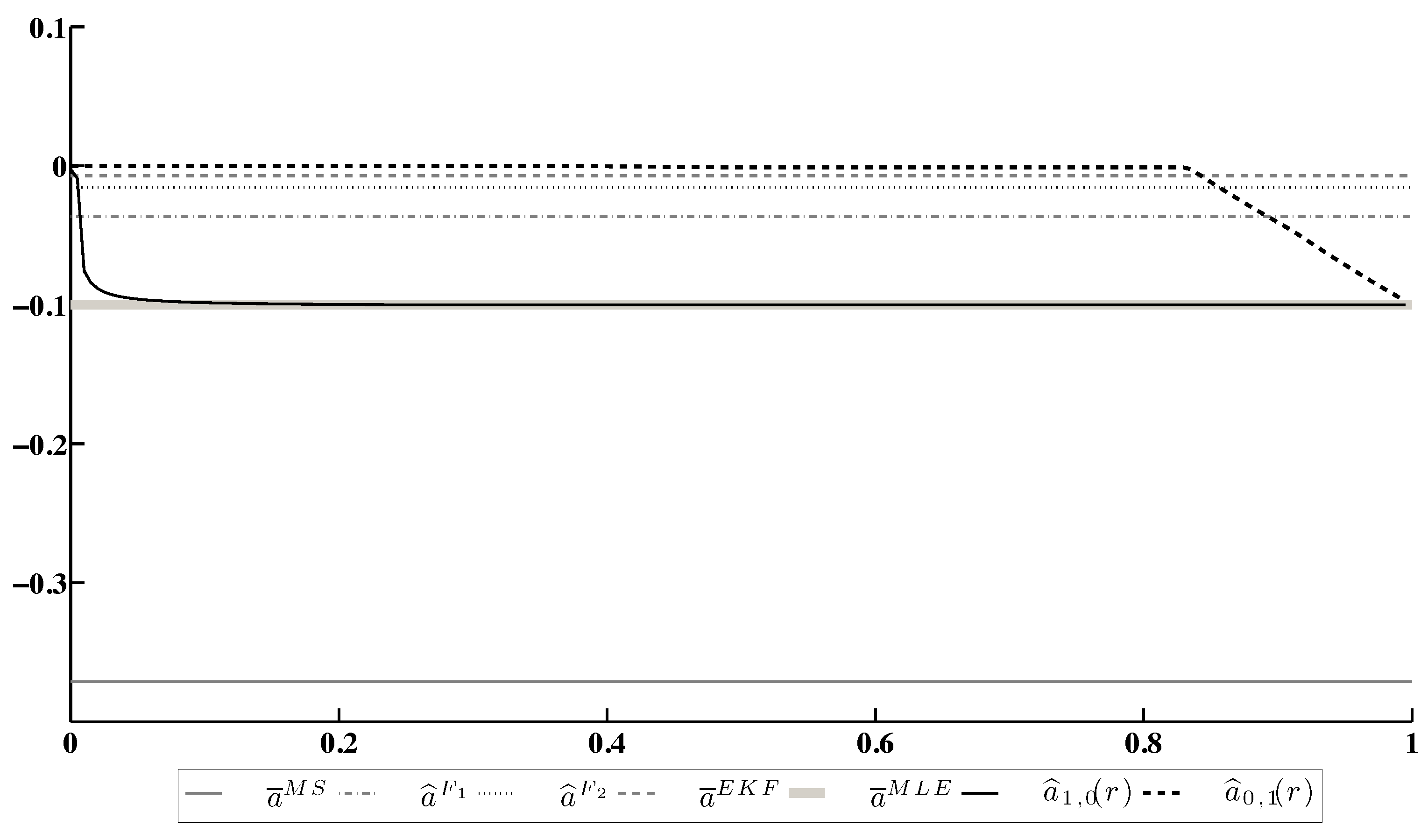
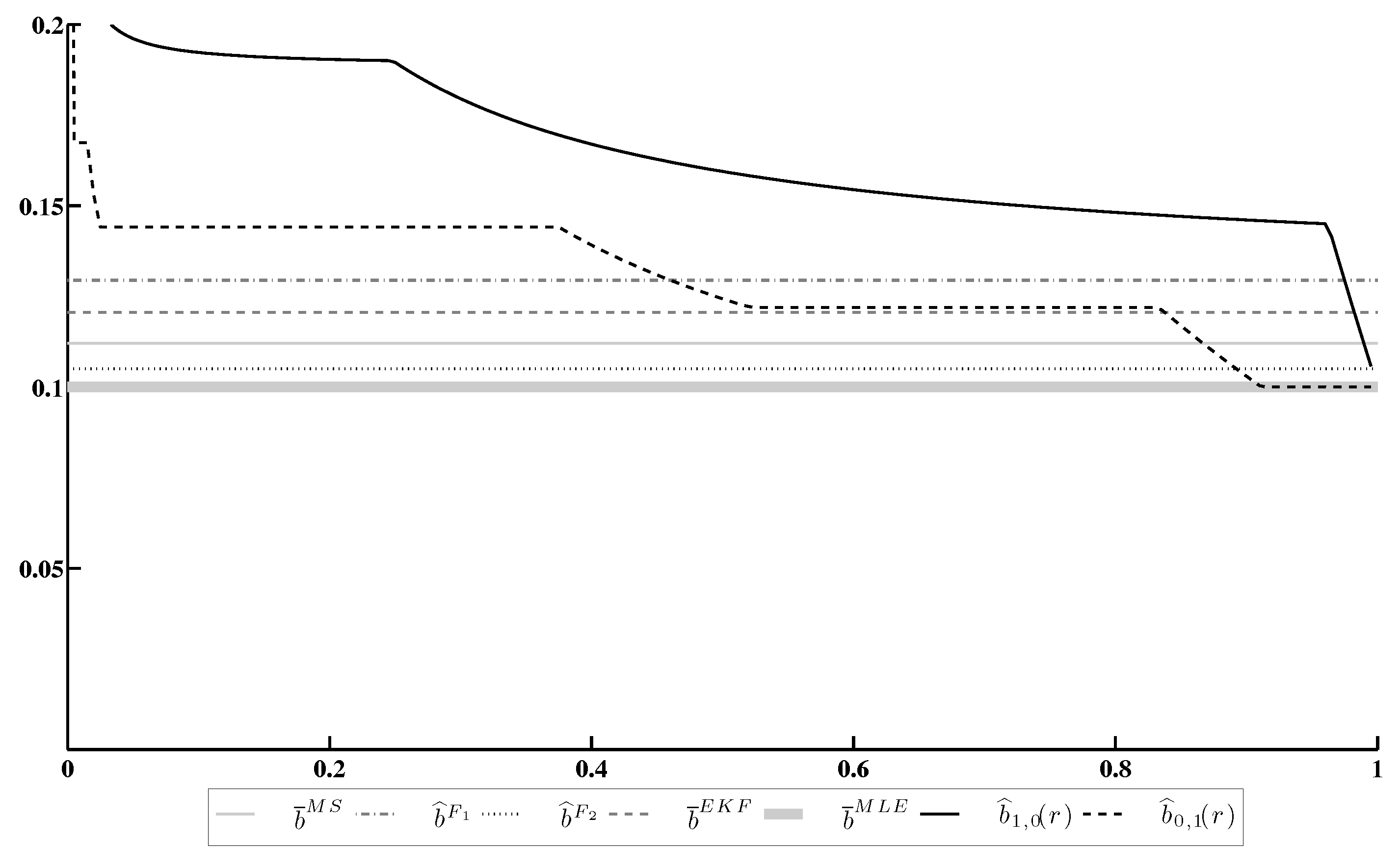
Figure 1 presents the evolution of the minimax estimates ${\widehat{a}}_{0,1}\left(r\right)$ and ${\widehat{a}}_{1,0}\left(r\right)$ of a drift coefficient depending on the confidence ratio $r\in (0,1)$. The minimax estimates are compared with;

• The estimate ${\overline{a}}^{MS}\left(Y_T\right)$ calculated by the moment/substitution method [12]:

  $$\begin{array}{cc}{\displaystyle {\overline{a}}^{MS}=\sum _{t=1}^T{y}_{t-1}{y}_t/(\sum _{t=1}^T{y}_t^2-T{f}^2),}\hfill & \hfill {\displaystyle {\overline{b}}^{MS}=\sqrt{{\displaystyle \frac{1}{c^2}\left(1-{\left({\overline{a}}^{MS}\right)}^2\right)(\sum _{t=1}^T{y}_t^2-T{f}^2)}};}\end{array}$$
• The Bayesian estimate ${\widehat{a}}^{F_1}\left({\mathbf{Y}}_T\right)$ (11) calculated under the assumption that prior distribution $F_1$ of $\gamma$ is uniform over the whole uncertainty set $\mathcal{C}$;
• The Bayesian estimate ${\widehat{a}}^{F_2}\left({\mathbf{Y}}_T\right)$ (11) calculated under the assumption that the prior distribution $F_2$ of $\gamma$ is uniform over the vertices of $\mathcal{C}$;
• The estimate ${\overline{a}}^{EKF}\left({\mathbf{Y}}_T\right)$ calculated by the extended Kalman filter (EKF) algorithm [39] and subsequent residual processing;
• The maximum likelihood estimate (MLE) ${\overline{a}}^{MLE}\left({\mathbf{Y}}_T\right)$ calculated by the expectation/maximization algorithm (EM algorithm) [17].

Figure 2 contains a similar comparison of the diffusion coefficient estimates ${\widehat{b}}_{0,1}\left(r\right)$ and ${\widehat{b}}_{1,0}\left(r\right)$.

The results of this experiment allow us to make the following conclusions.

• Both minimax estimates $({\widehat{a}}_{0,1}\left(r\right),{\widehat{b}}_{0,1}\left(r\right))$ and $({\widehat{a}}_{1,0}\left(r\right),{\widehat{b}}_{1,0}\left(r\right))$ converge to the MLE $({\overline{a}}^{MLE},{\overline{b}}^{MLE})$ as $r\to 1$. Nevertheless, the rate of convergence depends on the specific choice of the loss function ($J_{0,1}$ or $J_{1,0}$ in the considered case).
• Both minimax estimates are more conservative than the MLE, because they take into account a chance for other points of the LFD domain to be realized.
• Under an appropriate choice of the confidence ratio r, both minimax estimates become more accurate than other candidates, except for the MLE.

5.2. Parameter Estimation under Additive and Multiplicative Observation Noises

We consider the observations ${\mathbf{Y}}_T\triangleq col(Y_1,\dots ,Y_T)$:

$$Y_t=a{X}_t+V_t,t=\overline{1,T}.$$

(44)

Here:

• a is an estimated value;
• ${\mathbf{X}}_T\triangleq col(X_1,\dots ,X_T)$ is a vector of the i.i.d. unobservable random values (multiplicative noise): $X_1\sim \mathcal{R}[0,1]$;
• ${\mathbf{V}}_T\triangleq col(V_1,\dots ,V_T)$ is a vector of the i.i.d. unobservable random values (additive noise): $V_1\sim \mathcal{N}(0,\sigma )$.

We assume that the parameter a is random with unknown distribution, whose support set lies within the known set $\mathcal{C}\triangleq [c^1,c^2]$. The loss function has the form:

$$J(\overline{a},F|{\mathbf{Y}}_T)={\mathsf{E}}_F\left\{\parallel a-\overline{a}\left({\mathbf{Y}}_T\right){\parallel }^2|{\mathbf{Y}}_T\right\}.$$

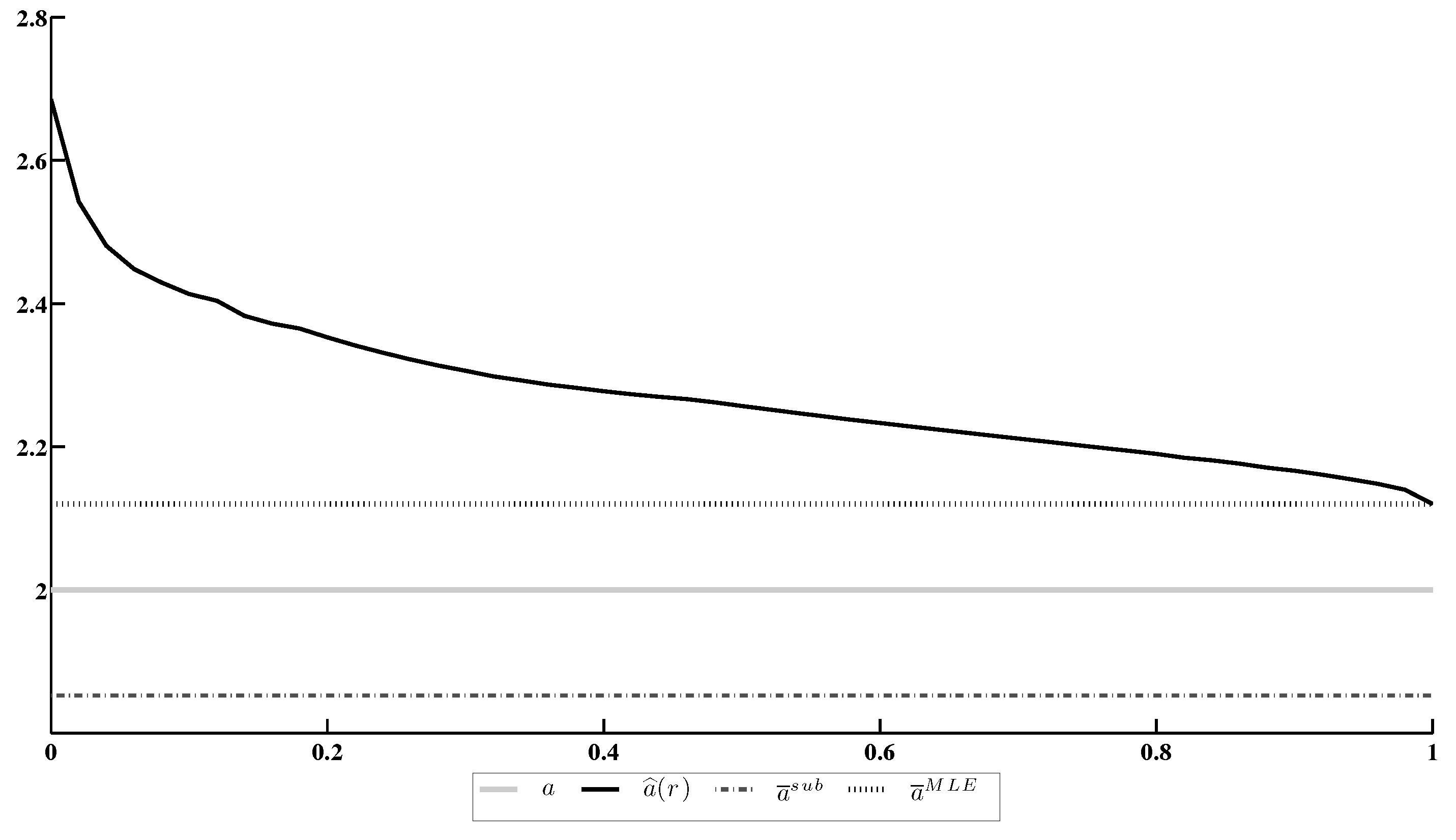
In this example our goal is to compare the minimax estimates of the parameter a under conformity constraint based either on the likelihood function or on the EDF.

The minimax estimations are calculated for the following parameter values: $a=2$, $T=20$, $\mathcal{C}=[2,3]$, $\sigma =0.1$. We use the proposed numerical procedure under a uniform mesh ${\mathcal{C}}_h$ of the set $\mathcal{C}$ with the step $h=0.005$. The example has some features. First, the observation model contains both the additive (${\mathbf{V}}_T$) and multiplicative (${\mathbf{X}}_T$) heterogeneous noises. Second, the available observed sample is not too long to provide the high quality for the consistent estimates. Third, the exact value of a is equal 2; meanwhile under the constraint absence there exists a discrete variant of the LFD with the finite support set $\{2,3\}$. This means that the LFD is realized only in the considered observation model.

The likelihood conformity constraint looks similar to the one from the previous subsection:

$${\displaystyle \frac{\mathfrak{L}({\mathbf{Y}}_T,F)-{min}_{q\in {\mathcal{C}}_h}\mathcal{L}\left({\mathbf{Y}}_T\right|q)}{{max}_{q\in {\mathcal{C}}_h}\mathcal{L}\left({\mathbf{Y}}_T\right|q)-{min}_{q\in {\mathcal{C}}_h}\mathcal{L}\left({\mathbf{Y}}_T\right|q)}⩾r,}$$

(45)

where $r\in (0,1)$ is a confidence ratio.

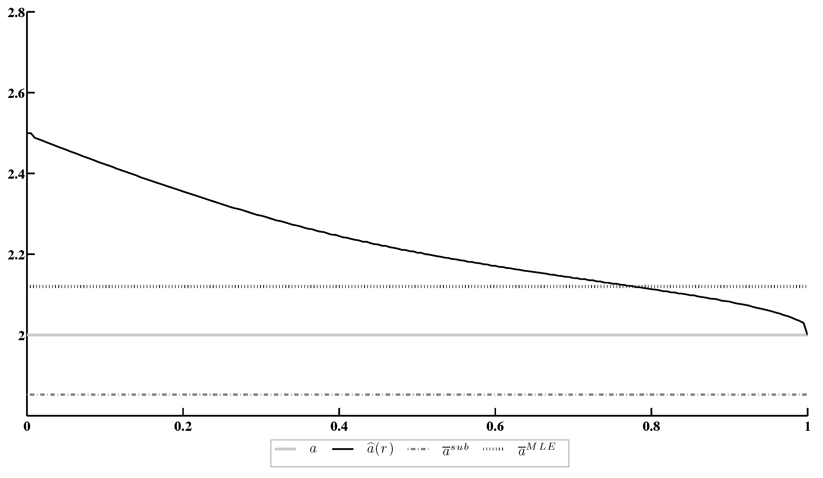
Figure 3 contains comparison of the minimax estimate $\widehat{a}\left(r\right)$ with its actual value a, the (consistent asymptotically Gaussian) M-estimate ${\overline{a}}^{sub}\triangleq \frac{2}{T}{\sum }_{t=1}^T{Y}_t$, obtained by the moment/substitution method [12] and the MLE ${\overline{a}}^{MLE}$.

Next, we investigate minimax posterior estimates under the conformity constraint based on the EDF. The constraint is of the form:

$$\frac{{max}_{F\in {\mathbb{F}}_{{\mathcal{C}}_h}}\mathfrak{M}({\mathbf{Y}}_T,F)-\mathfrak{M}({\mathbf{Y}}_T,F)}{{max}_{F\in {\mathbb{F}}_{{\mathcal{C}}_h}}\mathfrak{M}({\mathbf{Y}}_T,F)-{min}_{F\in {\mathbb{F}}_{{\mathcal{C}}_h}}\mathfrak{M}({\mathbf{Y}}_T,F)}⩾r,$$

(46)

where $r\in (0,1)$ is some fixed confidence ratio, and ${\mathbb{F}}_{{\mathcal{C}}_h}$ is a “mesh” approximation of the set ${\mathbb{F}}_{\mathcal{C}}$ corresponding to the uniform “mesh” ${\mathcal{C}}_h$. The form (46) of the conformity constraint provides that it is active in the minimax optimization problem for any $r\in (0,1)$.

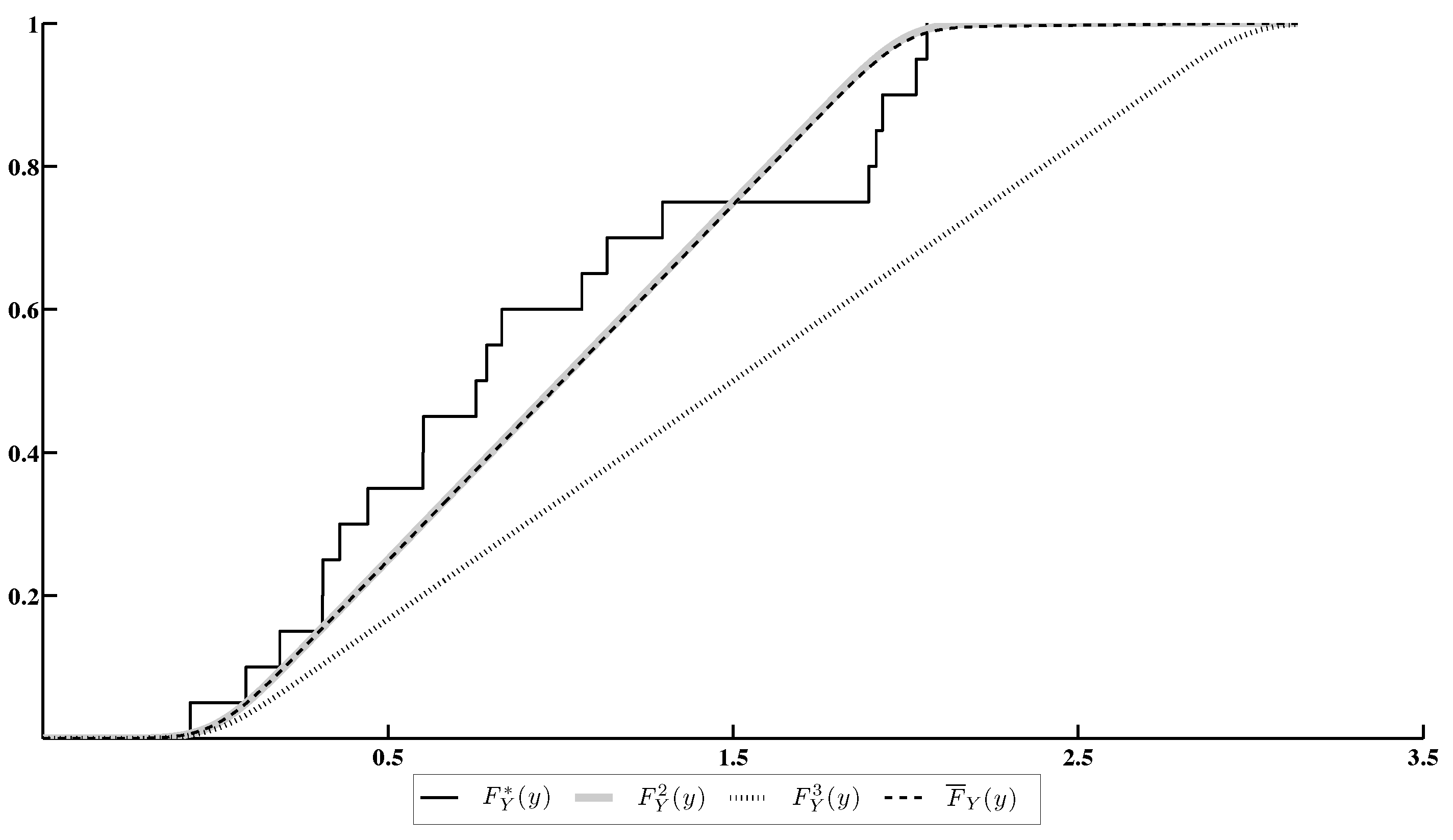
Figure 4 contains:

• The EDF $F_Y^{*}\left(y\right)$ calculated by the sample ${\mathbf{Y}}_T$;
• The cdf’s $F_Y^q\left(y\right)={\int }_{-\infty }^y{\varphi }_V\left(\frac{u-A\left(q\right)}{B\left(q\right)}\right)du$ of Y, corresponding to the one-point distribution concentrated at the point q ($q=2,3$);
• The cdf ${\overline{F}}_Y\left(y\right)$ ${\overline{F}}_Y\left(y\right)\in {\mathrm{Argmin}}_{F\in {\mathbb{F}}_{{\mathcal{C}}_h}}\mathfrak{M}({\mathbf{Y}}_T,F)$, closest to the EDF $F_Y^{*}\left(y\right)$ within the set ${\mathbb{F}}_{{\mathcal{C}}_h}$.

Note that $F_Y^2\left(y\right)$ is a cdf of Y corresponding to the actual value of a.

Figure 5 contains a comparison of the minimax estimate $\widehat{a}\left(r\right)$ under the conformity constraint, based on the EDF, with its actual value a, the moment/substitution estimate ${\displaystyle {\overline{a}}^{sub}}$ and the MLE ${\overline{a}}^{MLE}$.

The results of this experiment allow us to make the following conclusions.

• The minimax estimate $\widehat{a}\left(r\right)$ under the conformity constraint, based on the EDF, does not converge to the MLE ${\overline{a}}^{MLE}$ as $r\to 1$.
• Under an appropriate choice of the confidence ratio r, the minimax estimate under the EDF constraint becomes more accurate than other candidates, including the MLE.

6. Conclusions

The paper contains the statement and solution to a new minimax estimation problem for the uncertain stochastic regression parameters. The optimality criterion is the conditional mean square of the estimation error given the realized observations. The class of admissible estimators contains all (linear and nonlinear) statistics with finite variance. The a priori information concerning the estimated vector is incomplete: the vector is random and the part of its components lies in the known compact. The key feature of the considered problem is the presence of the additional constraints for the statistical uncertainty, restricting from below the correspondence degree between the uncertainty and realized observations. The paper presents various indices, characterizing this conformity via the likelihood function, the EDF and the sample mean.

We propose a reduction of the initial optimization problem in the abstract infinite-dimensional spaces to the standard finite-dimensional QP problem with convex constraints along with an algorithm of its numerical realization and precision analysis.

The minimax estimation problem is solved in terms of the saddle points, i.e., besides the estimators with the guaranteed quality, we have a description of the LFDs. First, the investigation of the LFDs’ domains allowed us the detection of the uncertain parameter values, which are the worst for the estimation. Second, the consideration of the performance index pair “conformity index–guaranteed estimation quality” uncovered rather a new conception of the parameter estimation under a vector optimality criterion. The paper contains an assertion, which states that the LFDs are Pareto-optimal for the vector-valued criterion above.

The paper focuses mostly on the conformity indices related to the likelihood function; thus, it is obvious that the performance of the minimax estimate is compared with the one of the MLE. In general, the MLE has several remarkable properties, in particular the asymptotic minimaxity under some additional restrictions [12]. However, the estimate is non-robust to the prior statistical uncertainty. The proposed minimax estimate can be considered as a robustified version of the MLE, which is ready for application in the cases of the short non-asymptotic samples or the violation of the conditions for the MLE asymptotic minimaxity.

The conformity constraints are not exhausted by the likelihood function. In the paper, we present other conformity indices based on the EDF and sample mean. We demonstrate that the minimax estimates with the EDF conformity constraint are better than the MLE. One of the points of the paper is that the flexible choice of the conformity indices and design of the additional conformity constraints for each individual applied estimation problem allows obtaining a tradeoff between the prior uncertainty and available observations.

The reason to choose one or another conformity index depends not only on the conditions of the specific practical estimation problem solved under the minimax settings. One of the essential conditions is the possibility of its quick computation for the subsequent verification of the conformity constraint. For example, calculation of the likelihood conformity constraint (33) with the guess value $\mathcal{L}\left(y\right|\overline{q})={max}_q\mathcal{L}\left(y\right|q)$ tends to necessarily solve the auxiliary maximization problem for the likelihood function, which is nontrivial itself. Thus, the conformity indices based on the EDF or sample moments look more prospective from the computational point of view.

The applicability of the proposed minimax estimate also depends on the presence of the analytical formula of the estimates $w\left(y\right|q)$, or the fast numerical algorithms of its calculation. In turn, this possibility is a base for the subsequent effective solution to the QP problem and specification of the LFD.

Finally, the key indicator affecting the estimate calculation process and its precision is the number of the mesh nodes in the approximation $\mathcal{C}\left({ϵ}_n\right)$ of the uncertainty set $\mathcal{C}$. It is a function of “the size of $\mathcal{C}$ / the mesh step ${ϵ}_n$′ ratio and dimensionality m of $\mathcal{C}$.

All of the factors above characterize the limits of possible applicability of the proposed minimax estimation method for the solution to one or another practical problem.

References

- Calafiore, G.; El Ghaoui, L. Robust maximum likelihood estimation in the linear model. Automatica 2001, 37, 573–580. [Google Scholar] [CrossRef]
- Kurzhanski, A.B.; Varaiya, P. Dynamics and Control of Trajectory Tubes; Birkhäuser: Basel, Switzerland, 2014. [Google Scholar]
- Matasov, A. Estimators for Uncertain Dynamic Systems; Kluwer: Dortrecht, The Netherlands, 1998. [Google Scholar]
- Borisov, A.V.; Pankov, A.R. Optimal filtering in stochastic discrete-time systems with unknown inputs. IEEE Trans. Autom. Control 1994, 39, 2461–2464. [Google Scholar] [CrossRef]
- Pankov, A.R.; Semenikhin, K.V. Minimax identification of a generalized uncertain stochastic linear model. Autom. Remote Control 1998, 59, 1632–1643. [Google Scholar]
- Poor, V.; Looze, D. Minimax state estimation for linear stochastic systems with noise uncertainty. IEEE Trans. Autom. Control 1981, 26, 902–906. [Google Scholar] [CrossRef]
- Soloviev, V. Towards the Theory of Minimax-Bayesian Estimation. Theory Probab. Its Appl. 2000, 44, 739–754. [Google Scholar] [CrossRef]
- Blackwell, D.; Girshick, M. Theory of Games and Statistical Decisions; Wiley: New York, NY, USA, 1954. [Google Scholar]
- Martin, C.; Mintz, M. Robust filtering and prediction for linear systems with uncertain dynamics: A game-theoretic approach. IEEE Trans. Autom. Control 1983, 28, 888–896. [Google Scholar] [CrossRef]
- Berger, J.O. Statistical Decision Theory and Bayesian Analysis; Springer: Berlin/Heidelberg, Germany, 1985. [Google Scholar]
- Anan’ev, B. Minimax Estimation of Statistically Uncertain Systems Under the Choice of a Feedback Parameter. J. Math. Syst. Estim. Control 1995, 5, 1–17. [Google Scholar]
- Borovkov, A. Mathematical Statistics; Australia Gordon & Breach: Blackburn, Australia, 1998. [Google Scholar]
- Epstein, L.; Ji, S. Ambiguous volatility, possibility and utility in continuous time. J. Math. Econ. 2014, 50, 269–282. [Google Scholar] [CrossRef] [Green Version]
- Borisov, A.V. A posteriori minimax estimation with likelihood constraints. Autom. Remote Control 2012, 73, 1481–1497. [Google Scholar] [CrossRef]
- Arkhipov, A.; Semenikhin, K. Minimax Linear Estimation with the Probability Criterion under Unimodal Noise and Bounded Parameters. Autom. Remote Control 2020, 81, 1176–1191. [Google Scholar] [CrossRef]
- Germeier, Y. Non-Antagonistic Games; Springer: New York, NY, USA, 1986. [Google Scholar]
- Elliott, R.J.; Moore, J.B.; Aggoun, L. Hidden Markov Models: Estimation and Control; Springer: New York, NY, USA, 1995. [Google Scholar]
- Yosida, K. Functional Analysis; Grundlehren der Mathematischen Wissenschaften; Springer: Berlin/Heidelberg, Germany, 2013. [Google Scholar]
- Liptser, R.; Shiryaev, A. Statistics of Random Processes: I. General Theory; Springer: Berlin/Heidelberg, Germany, 2001. [Google Scholar]
- Kats, I.; Kurzhanskii, A. Estimation in Multistep Systems. Proc. USSR Acad. Sci. 1975, 221, 535–538. [Google Scholar]
- Petersen, I.R.; James, M.R.; Dupuis, P. Minimax optimal control of stochastic uncertain systems with relative entropy constraints. IEEE Trans. Autom. Control 2000, 45, 398–412. [Google Scholar] [CrossRef] [Green Version]
- Xie, L.; Ugrinovskii, V.A.; Petersen, I.R. Finite horizon robust state estimation for uncertain finite-alphabet hidden Markov models with conditional relative entropy constraints. In Proceedings of the 2004 43rd IEEE Conference on Decision and Control (CDC) (IEEE Cat. No.04CH37601), Nassau, Bahamas, 14–17 December 2004; Volume 4, pp. 4497–4502. [Google Scholar] [CrossRef]
- El Karoui, N.; Jeanblanc Picque, M. Contrôle de processus de Markov. Séminaire Probab. Strasbg. 1988, 22, 508–541. [Google Scholar]
- Lee, E.; Markus, L. Foundations of Optimal Control Theory; SIAM Series in Applied Mathematics; Wiley: Hoboken, NJ, USA, 1967. [Google Scholar]
- Floyd, S.; Jacobson, V. Random early detection gateways for congestion avoidance. IEEE/ACM Trans. Netw. 1993, 1, 397–413. [Google Scholar] [CrossRef]
- Low, S.H.; Paganini, F.; Doyle, J.C. Internet congestion control. IEEE Control Syst. Mag. 2002, 22, 28–43. [Google Scholar] [CrossRef] [Green Version]
- Altman, E.; Avrachenkov, K.; Menache, I.; Miller, G.; Prabhu, B.J.; Shwartz, A. Dynamic Discrete Power Control in Cellular Networks. IEEE Trans. Autom. Control 2009, 54, 2328–2340. [Google Scholar] [CrossRef]
- Perruquetti, W.; Barbot, J.P. Sliding Mode Control in Engineering; Marcel Dekker, Inc.: New York, NY, USA, 2002. [Google Scholar]
- Arnold, B.F.; Stahlecker, P. Fuzzy prior information and minimax estimation in the linear regression model. Stat. Pap. 1997, 38, 377–391. [Google Scholar] [CrossRef]
- Donoho, D.; Johnstone, I.; Stern, A.; Hoch, J. Does the maximum entropy method improve sensitivity? Proc. Natl. Acad. Sci. USA 1990, 87, 5066–5068. [Google Scholar] [CrossRef] [PubMed] [Green Version]
- Donoho, D.L.; Johnstone, I.M.; Hoch, J.C.; Stern, A.S. Maximum Entropy and the Nearly Black Object. J. R. Stat. Society. Ser. B 1992, 54, 41–81. [Google Scholar] [CrossRef]
- Pham, D.S.; Bui, H.H.; Venkatesh, S. Bayesian Minimax Estimation of the Normal Model with Incomplete Prior Covariance Matrix Specification. IEEE Trans. Inf. Theory 2010, 56, 6433–6449. [Google Scholar] [CrossRef] [Green Version]
- Donoho, D.L.; Johnstone, I.M. Minimax risk over lp-balls for lq-error. Probab. Theory Relat. Fields 1994, 99, 277–303. [Google Scholar] [CrossRef]
- Donoho, D.L.; Johnstone, I.M. Minimax estimation via wavelet shrinkage. Ann. Stat. 1998, 26, 879–921. [Google Scholar] [CrossRef]
- Donoho, D.L.; Johnstone, I.; Montanari, A. Accurate Prediction of Phase Transitions in Compressed Sensing via a Connection to Minimax Denoising. IEEE Trans. Inf. Theory 2013, 59, 3396–3433. [Google Scholar] [CrossRef] [Green Version]
- Bosov, A.; Borisov, A.; Semenikhin, K. Conditionally Minimax Prediction in Nonlinear Stochastic Systems. IFAC-PapersOnLine 2015, 48, 802–807. [Google Scholar] [CrossRef]
- Kadets, V. A Course in Functional Analysis and Measure Theory; Springer: Berlin/Heidelberg, Germany, 2018. [Google Scholar]
- Gelman, A.; Carlin, J.B.; Stern, H.S.; Rubin, D.B. Bayesian Data Analysis, 2nd ed.; Chapman and Hall/CRC: London, UK, 2004. [Google Scholar]
- Anderson, B.; Moore, J. Optimal Filtering; Prentice-Hall: Upper Saddle River, NJ, USA, 1979. [Google Scholar]
- Grabiner, J.; Balakrishnan, A. Applications of Mathematics: Applied Functional Analysis; Applications of Mathematics; Springer: New York, NY, USA, 1981. [Google Scholar]
Figure 1.
Estimation of the drift coefficient a.
Figure 2.
Estimation of the diffusion coefficient b.
Figure 3.
Estimation of the coefficient a under conformity constraint based on the likelihood function.
Figure 4.
The EDF of Y and different cdf’s of Y under various choices of a.
Figure 5.
Estimation of the coefficient a under conformity constraint based on the EDF.
Publisher’s Note: MDPI stays neutral with regard to jurisdictional claims in published maps and institutional affiliations. |
© 2021 by the author. Licensee MDPI, Basel, Switzerland. This article is an open access article distributed under the terms and conditions of the Creative Commons Attribution (CC BY) license (https://creativecommons.org/licenses/by/4.0/).
Share and Cite
MDPI and ACS Style
Borisov, A. Minimax Estimation in Regression under Sample Conformity Constraints. Mathematics 2021, 9, 1080. https://doi.org/10.3390/math9101080
AMA Style
Borisov A. Minimax Estimation in Regression under Sample Conformity Constraints. Mathematics. 2021; 9(10):1080. https://doi.org/10.3390/math9101080
Chicago/Turabian StyleBorisov, Andrey. 2021. "Minimax Estimation in Regression under Sample Conformity Constraints" Mathematics 9, no. 10: 1080. https://doi.org/10.3390/math9101080
Note that from the first issue of 2016, this journal uses article numbers instead of page numbers. See further details here.