
The Modulation Effect on the ELVEs and Sprite Halos by Concentric Gravity Waves Based on the Electromagnetic Pulse Coupled Model

1
College of Air Traffic Management, Civil Aviation Flight University of China, Guanghan 618307, China
2
School of Computer Science and Communication Engineering, Jiangsu University, Zhenjiang 212013, China
3
School of Atmospheric Physics, Nanjing University of Information Science and Technology, Nanjing 210044, China
4
College of Fisheries, Guangdong Ocean University, Zhanjiang 524088, China
*
Authors to whom correspondence should be addressed.
Atmosphere 2021, 12(5), 617; https://doi.org/10.3390/atmos12050617
Submission received: 12 April 2021
/
Revised: 5 May 2021
/
Accepted: 6 May 2021
/
Published: 11 May 2021
(This article belongs to the Special Issue Atmospheric Electricity)
Abstract
:By employing the finite-difference time-domain method, the processes of electric field variation and morphological development of the optical radiation field of ELVEs and sprite halos were simulated in this article. Simulations of ELVEs show two optical radiation field centers, with a concentrated luminous zone from 85 to 100 km and an inner weaker optical radiation center. The electric field exhibits an obvious sparse and dense ripple pattern induced by the concentric gravity waves (CGWs) at altitudes of 90–100 km, which mainly occurs during the decline period of electric field with a shallow steepness. The alternating distance of the variations in the sparse and dense patterns is about 40 km, which corresponds to the horizontal wavelength of the electric field. The CGWs induce significant deformation of the inner optical radiation field, even splitting into multiple luminous regions. Simulations of sprite halos indicate that the horizontal range of the electrical field generated by lightning current is within 50 km, and a strong local electric field formed in the region right above the lightning channel is due to the small-scale breakdown current. Thus, the increased electron density shields the upper regions and reduces the electrical field’s strength. The sprite halos luminous zone is pancake-shaped, and it originates at 85 km along with a downward developing trend. The disturbance of sprite halos’ luminescence caused by CGWs mainly occurs at about 80–100 km directly above the lightning channel, and the primary deformation zone is located within 30 km of the lightning channel, which is also the region with the most recognizable electric field disturbance.
1. Introduction
Transient luminous events (TLEs) at mid-to-high altitudes are the luminescence caused by the disruptive discharge of the neutral rarefied atmosphere, which are induced by the electromagnetic pulse (EMP) generated by the tropospheric lightning activity [1,2]. This electromagnetic activities in the stratosphere and mesosphere may have potential influences on global circuits, atmospheric photochemical effects at high altitudes, electrodynamic coupling effects between the troposphere and mesosphere, and radio signal propagation in the lower ionosphere [3,4,5,6,7].
Red sprites (including sprite halos), blue jets, gigantic jets and emissions of light, and very low frequency (VLF) perturbation due to electromagnetic pulse Sources (ELVEs), are four common types of TLEs [8,9]. ELVEs circular disk or cyclic infrared radiation phenomenon, for a short duration of less than ~1 ms, is the most frequent TLE (six-times that of sprites) in the world, with the highest occurrence position of 90–100 km and the largest horizontal scale of 200–600 km [10]. Based on observations, Taranenko et al. [11] have found that a fraction of strong electromagnetic pulses triggered by the lightning-return-stroke large-current process in the troposphere can penetrate the lower ionosphere and induce electronic disturbance, then the electrons are heated to produce ELVEs. Sprite halos (referred to halos) tend to be born at an altitude of 70–85 km, resembling a thin pancake red diffuse glow, lasting approximately 1 ms [12]. In addition, halos can emerge alone, and when the distribution of electron density is uneven at the bottom of the ionosphere, the sprites will occur simultaneously. Existing research results show that the trigger mechanisms of ELVEs and sprites are mainly determined by two key factors: the strong electromagnetic pulse excited by the tropospheric lightning and the uneven electron density at the bottom of the ionosphere [13,14,15]. In the same electromagnetic environment, the increase of partial electron density (or inhomogeneous plasma density), is conducive to the formation of partial strong electric field, and then generating air breakdown discharge [16,17,18,19,20]. Moreover, the reduction of neutral air molecular density will significantly reduce the breakdown threshold due to the air breakdown discharge. After observations, Siefring et al. [21] pointed out that the TLEs frequently appear at the trough of OH airglow gravity waves at 80–90 km (corresponding to the trough of air density), and the smaller the air density, the more prone to breakdown discharge. Concentric gravity waves (CGWs) triggered by tropospheric thunderstorm activities can propagate upward to the lower ionosphere at 80–90 km, causing fluctuations in the spatial distribution of atmospheric electrical parameters in the present zone, which directly modulate the mid-to-high altitude TLEs (including ELVEs and sprite halos) occurring around current altitude [2,22,23,24].
At present, the modulation effect of gravity waves on the TLEs still remains at the theoretical research level. In 2015, Yue and Lyons [25] synchronously observed a typical case of thunderstorm concentric gravity waves propagating to the mid-to-high altitude regions and then conducted its parameterization analysis. Meanwhile, they also found that the CGWs had a profound modulation effect on ELVEs, forming striped ELVEs. Subsequently, Marshall et al. [26] simulated the effect of gravity waves on ELVEs phenomenon for the first time through an electromagnetic radiation model, which further confirmed that the striped ELVEs were the results of the modulation effect of gravity waves. Owing to the low capture probability and the difficulty of synchronous observation for the TLEs, few studies have systematically focused on the actual TLEs’ observations. Of particular note, the numerical simulation is still an effective method to analyze the modulation effect of gravity waves on TLEs. The electromagnetic pulse (EMP) model can accurately simulate the excitation process of ELVEs and halos by the electromagnetic radiation of the millisecond scale lightning return stroke [2].
Therefore, this article will establish the troposphere-middle upper altitudes EMP model based on the finite-difference time-domain method (FDTD). The simulation of the effects of gravity waves propagating to the mid-to-high altitude regions on the optical radiation phenomenon of ELVEs and sprite halos, and the space lightning electromagnetic field, will provide a theoretical reference to explain the correlation between gravity waves and the TLEs.
2. Establishment of Tropospheric Mid-to-High Altitude EMP Model
2.1. Introduction of 2D FDTD EMP Model
FDTD is an effective method to calculate the electromagnetic field of lightning. Since Yee [27] proposed the FDTD algorithm, the developed and improved FDTD algorithm has been widely applied to lightning electromagnetic field due to its flexible parameter setting and concise programming. Based on the time-domain Maxwell equation, the Yee cell which is the smallest unit of spatial meshwork, is taken as a spatial unit to discretize each component of the spatial electromagnetic field in time and space by means of the method of central difference. The obtained FDTD equation is iterated in time domain to solve the spatial electromagnetic field.
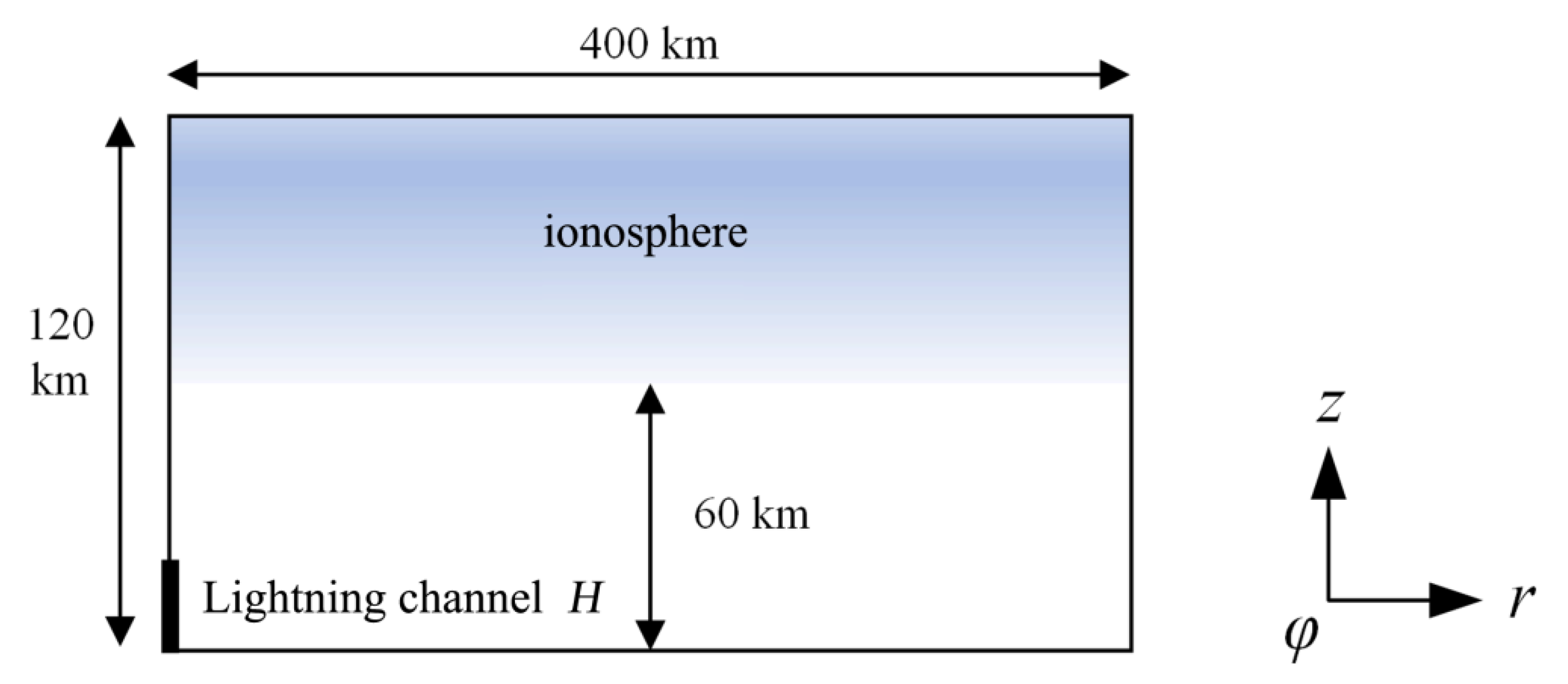
In this study, the FDTD algorithm is used to simulate the phenomenon of TLEs excited by the tropospheric lightning at mid-to-high altitudes, considering the effect of typical CGWs on the TLEs. As illustrated in Figure 1, due to the symmetry of the model, it can be established in two-dimensional cylindrical coordinates. The Radius r = 400 km, height z = 120 km, space step Δr = Δz = 1 km, and time step Δt = 16 ns of the whole simulated space satisfy the Courant stability conditions. The lightning return channel is located on the axis and the channel height H = 10 km. The model boundary adopts the first-order Mur absorption boundary.
For the atmosphere above a height of 60 km, owing to the gradual ionization of the solar radiation with height, the air conductivity gradually increases. Therefore, the simulation of the ionospheric areas needs to consider the influence of the air conductivity () in the lower-temperature plasma on the medium constitutive relation. Thus, in the two-dimensional FDTD model, the time-domain Maxwell equation is as follows [28,29]:
where and denote the electric field strength and magnetic induction strength respectively, is the total current density, the current density of excitation source (current density of lightning return stroke), the air conductivity, and and are the permittivity and permeability in vacuum, respectively. As shown in Figure 2, the three components of Er, Ez, and Bφ in the cylindrical coordinates are discretized by using the central difference method, and Equation (2) is obtained, which takes the form of:
where and denote horizontal and vertical electric field components, respectively, indicates the horizontal component of magnetic induction, c is the velocity of light in vacuum. The solution of Maxwell’s equations based on the iteration of Equation (2) is similar to that of a general FDTD algorithm. The distinction only lies in the calculation of the space conductivity. This parameter is not only related to the altitude, but also with the complicated nonlinear relationship. The interaction between various charged particles and electromagnetic fields in the ionosphere are eventually coupled into Maxwell’s equations through electrical conductivity. The calculation of conductivity involves ionospheric electrical parameters, such as electron density, electron mobility, ionization rate, and absorption rate, which will be introduced in detail in the following sections.
2.2. Calculation of Ionospheric Parameters
Under the influence of solar radiation, lower ionospheric air is a kind of lower-temperature plasma with weak ionization, and the air conductivity is produced by different charged particles, including ionic conductivity and electronic conductivity (). The ionic conductivity dominates the atmospheric conductivity below the altitude of 60 km, and its spatial distribution generally increases exponentially with altitude [30]. In this article, , where z represents altitude (units: km). In the lower ionospheric regions above 60 km, atmospheric conductivity is mainly composed of electronic conductivity, which takes the form of:
In Equation (3), indicates the amount of electron charge, denotes the electron number density, and is the electron mobility [31].
The electron number density satisfies the continuity equation, which can be expressed as:
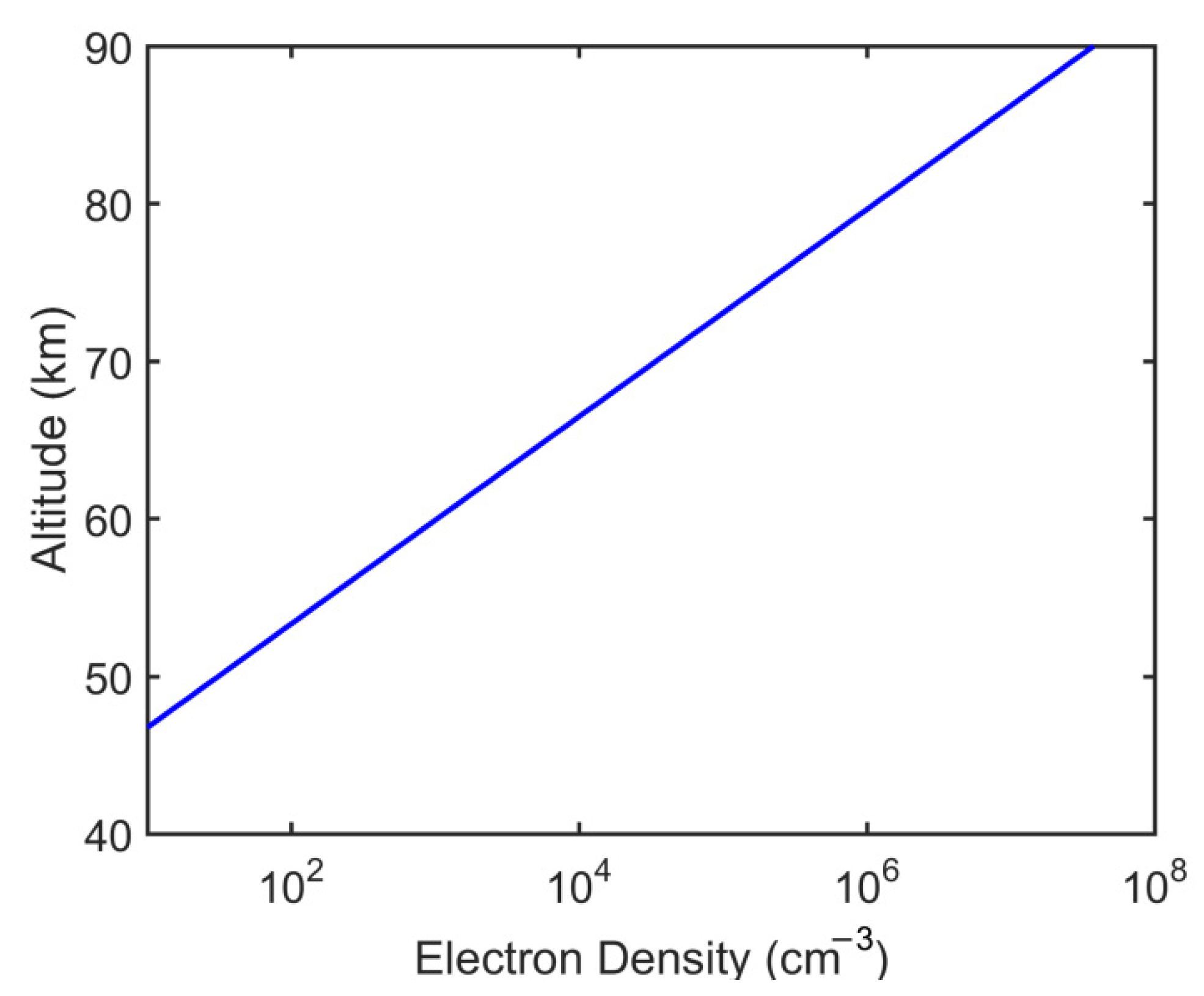
In this continuity equation, the initial value of electron number density is , where and reference height , as shown in Figure 3. Besides, and represent the ionization coefficient and the absorption coefficient, respectively, both of which are nonlinear functions of electric fields [32].
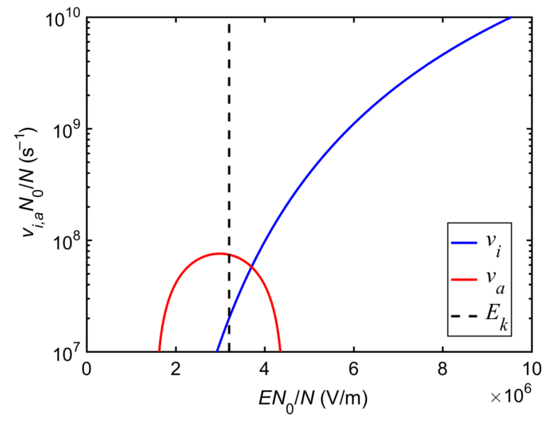
As illustrated in Figure 4, computational expression of ionization coefficient is as follows:
where , , , , , and and denote the atmospheric number density at the sea level and actual altitude respectively. , and is taken from the NRLMSISE-00 atmospheric parameter model.
The expression of absorption coefficient is [11]:
where , , , , , and .
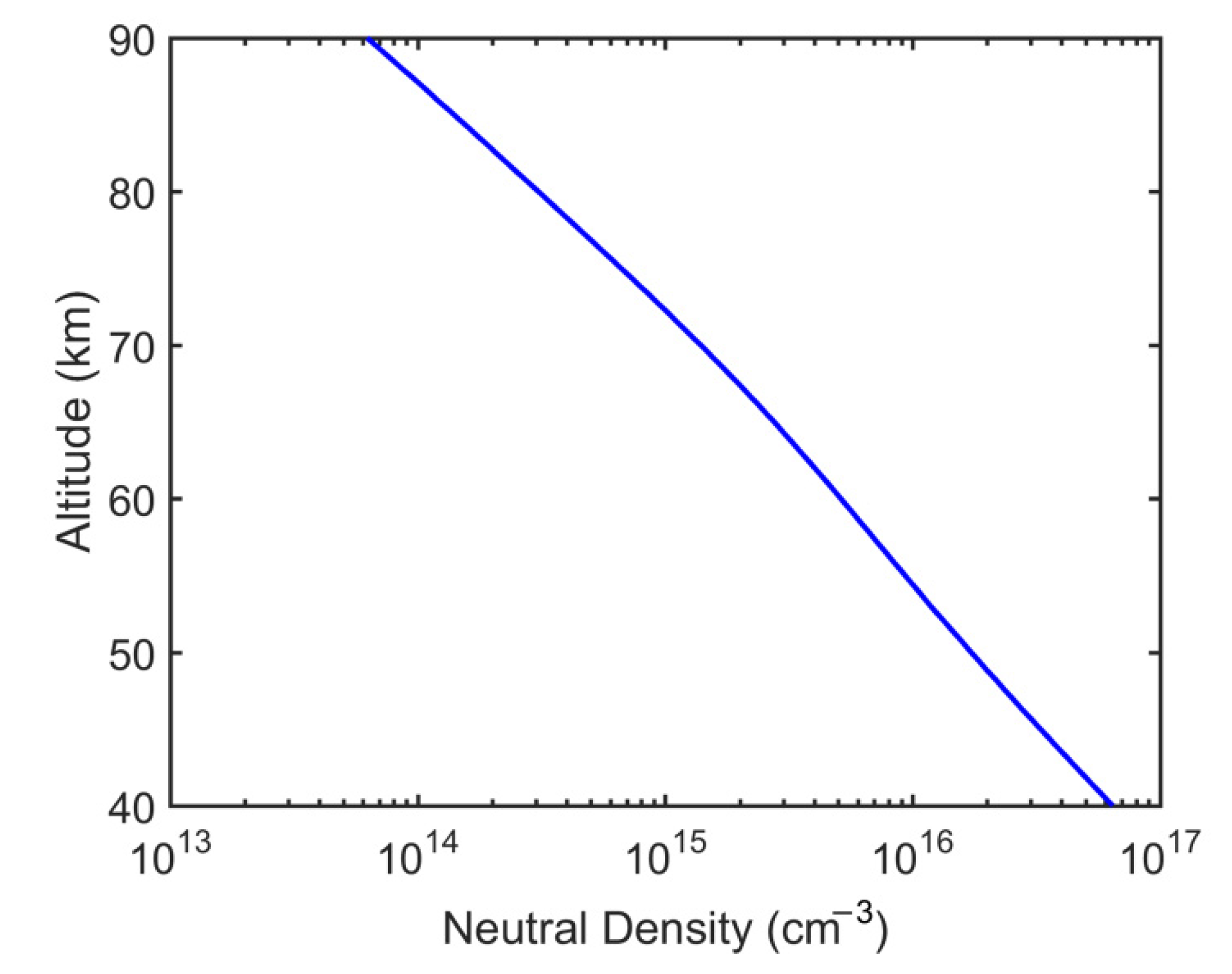
As shown in Figure 5, neutral air density is closely related to air breakdown threshold (). Based on the [33], the smaller the neutral air density is, the lower the breakdown threshold is, and the more easily air is broken down.
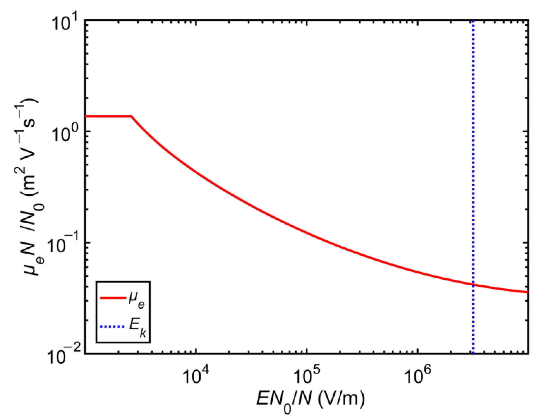
Electron mobility , as shown in Figure 6, varies non-linearly under the influence of electric fields [29].
In Equation (7), , , , and .
2.3. Calculation of Optical Radiation
As mentioned above, the spatial distribution characteristics of the lightning electromagnetic field affected by the ionospheric nonlinear effect can be calculated. Most of the actual TLEs’ phenomena at mid-to-high altitudes were observed by optical equipment, such as a low luminosity camera, etc. Thus, this study further simulates and calculates the optical radiation phenomenon for TLEs at the mid-to-high altitudes. The basic physical process is, the intense electric fields generated by lightning excite the atmospheric molecules, and when it returns to the ground state, the energy is transferred out by the optical radiation. Previous studies have revealed that the optical radiation effect of the first positive waveband of nitrogen molecules is dominant in the optical radiation of TLEs [2,10]. Therefore, only the first positive band of nitrogen molecules is calculated in this article.
Based on the calculation method of optical radiation given by Pasko et al. [8], the excitation rate is firstly calculated, which is related to electric field and neutral air density . Taranenko et al. [11] proposed an accurate analytical expression based on the experimental results, and its calculation formula is:
where and , the coefficient of the first positive band of the nitrogen molecule , , , and [34]. Then the molecular number densities in different bands during the excited state of k will be calculated, and the continuity equation is as follows:
where indicates the duration of excited state of k, denotes the transition coefficient, and are the number densities of N2 and O2, respectively, and are the quenching coefficients induced by the molecule colliding with N2 and O2, where , . represents the excitation process of electrons. Based on the calculated , the photon emission intensity () can be calculated, whose unit is [35].
2.4. Parameterization of CGWs
Considering the disturbance induced by atmospheric gravity waves to the lower ionospheric atmosphere, various studies pointed out different loading methods for this disturbance. For example, Qin et al. [36] have indicated that gravity waves could cause the nonuniformity and disturbance to the space electron density; Marshall et al. [26] have revealed that the middle and upper atmosphere density, particularly the neutral air density, would be disturbed by gravity waves. Rowland et al. [37] and Liu et al. [38] believed that the gravity waves would lead to the uneven distribution of ionization rates in the ionospheric atmosphere. The parameterization scheme of gravity waves spatial distribution proposed by Marshall et al. [26] based on the actual observations is applied to the loading of the gravity wave disturbance in current study. Introducing the effect of gravity waves by altering the spatial distribution of neutral air density, the neutral air density can be calculated by the equation as follows:
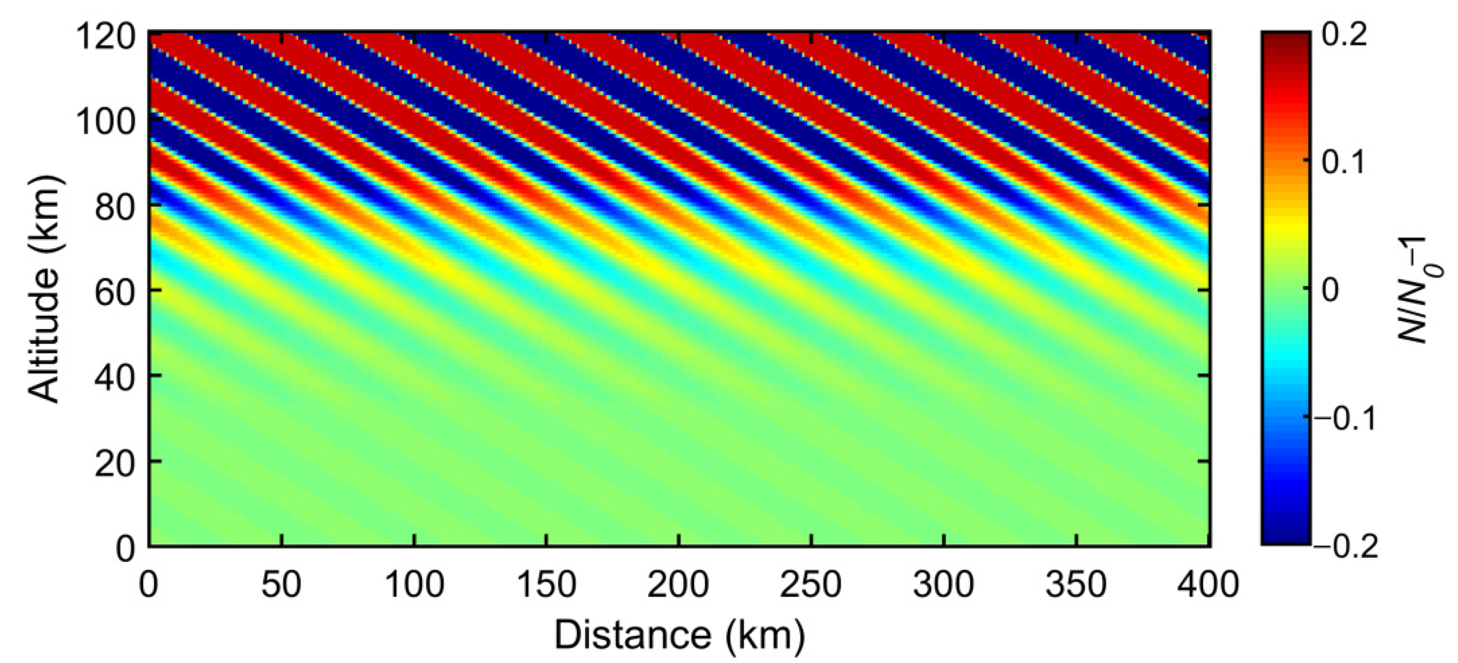
In Equation (10), denotes the background neutral air density, obtained from the NRLMSISE-00 atmospheric parameterization model. represents the peak altitude of disturbance, is the atmospheric elevation, and denotes the wave numbers of gravity waves in the direction of i (r or z). In the model of the current article, and represent the horizontal and vertical wavelengths being 40 and 15 km, respectively, which were observed by Yue and Lyons [25] and are used in the parameterized processing of the gravity wave by Marshall et al. [26]. A is the disturbance amplitude, and the value range is 0~40%. The perturbation method of electron density at mid-to-high altitudes by gravity wave is the same as that of . Figure 7 shows the spatial distribution of the relative variation of neutral air density N disturbed by atmospheric gravity wave when A = 20% (). Here, this article define that the relative variation of atmospheric density is A and −A correspond to the crest and trough of a gravity wave, respectively.
2.5. Algorithm Accuracy Verification
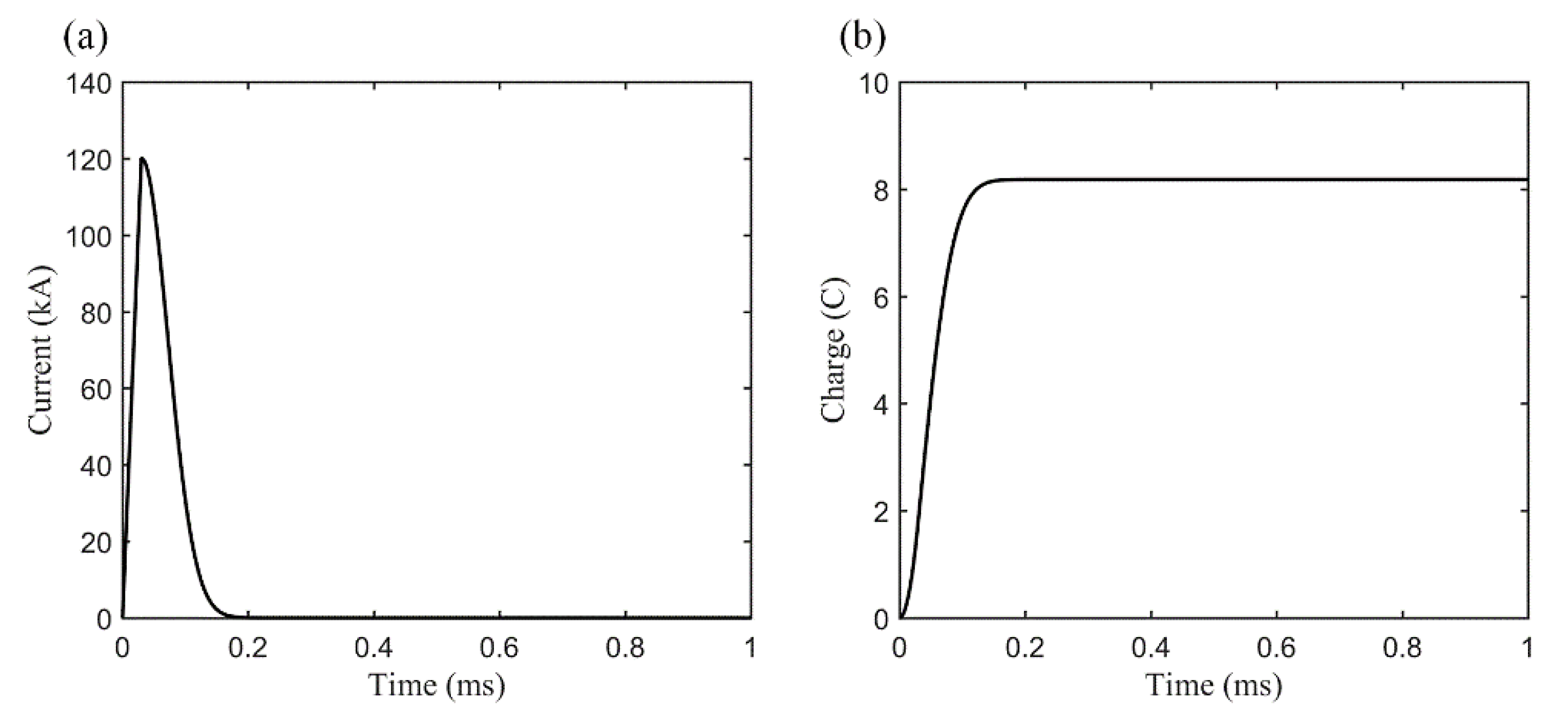
To verify the calculation accuracy of the 2-D FDTD electromagnetic radiation model, the contrastive analysis of simulation results, in this study and other existing studies, will be expounded. The peak value of lightning current is 120 kA, the waveform of rising edge time of 30 μs increased linearly, and the waveform of falling edge time of 60 μs decreased exponentially. The other parameters settings are as described above. Figure 8 presents the comparison results of the spatial distribution results of electric fields at different moments calculated by the 2-D model in this article and CP Barrington-Leigh [39] model, which shows a good consistency between these two models, confirming that the numerical model established in this article shows an accurate simulation accuracy.
3. Effect of Gravity Wave Disturbance on Mid-to-High Altitude ELVEs
3.1. Selection of Lightning Excitation Source
The phenomenon of ELVEs occurs at an altitude of about 85–95 km, for a short duration of less than ~1 ms. The formation of such a phenomenon is primarily due to air breakdown caused by the propagation of the radiation field toward mid-to-high altitudes, which is generated by the ground flashback. Thus, when simulating ELVEs, the lightning current waveform, which has a relatively large amplitude and distinct steepness, should be selected as the excitation source. This paper refers to the parametrization scheme of the 2D model of CP Barrington-Leigh [39] and adopts a lightning current waveform that increases linearly to a peak value and then exponentially decays, which takes the form of:
where represents the peak current (120 kA), and denote the rising edge and falling edge time of lightning current waveform, respectively, and their values are 30 μs and 60 μs, respectively. The lightning current waveform and corresponding amount of transferred charges are displayed in Figure 9a,b respectively.
3.2. Simulation Results
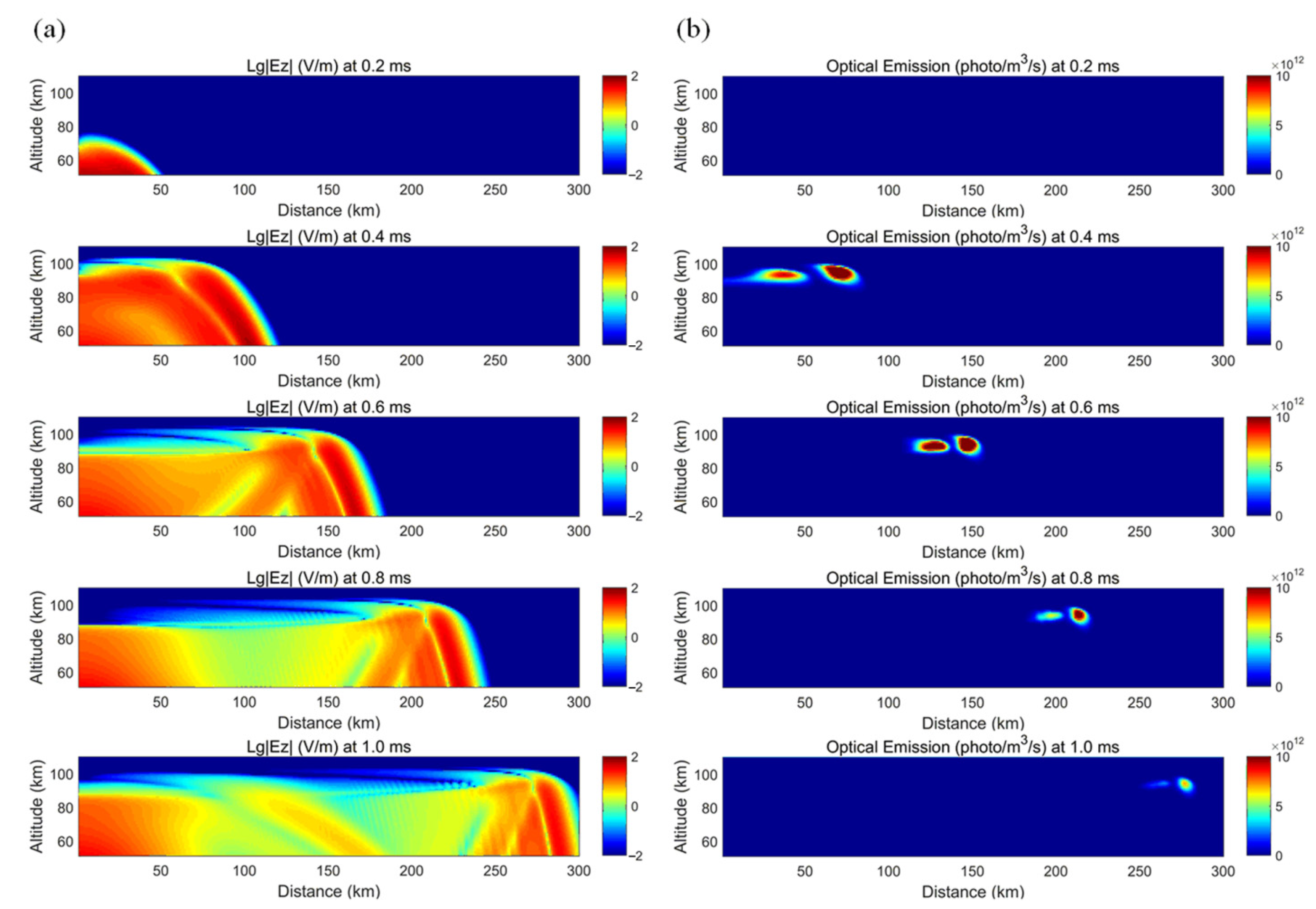
Figure 10 shows the calculated and simulated distribution of the spatial electric field caused by the lightning return current at mid-to-high altitudes and its corresponding optical emission of the excited ELVEs without gravity wave disturbance (i.e., disturbance amplitude A = 0%). Figure 10a shows the temporal and spatial evolution of the spatial electric field in the 50–110 km region. Because of the large difference between the far-field and near-field values, this study takes the logarithmic values of the electric field in order to capture the detailed variation characteristics in the electric field propagation. As can be seen in Figure 10, the spatial electric field propagates at the speed of light to a certain distance (mainly by the radiation field), and it has difficulty penetrating the ionosphere when it propagates to the lower ionosphere zone at mid-to-high altitudes because it is blocked by the ionosphere and produces an obvious reflection. The electric fields are primarily concentrated below 100 km. The electric field, which is close to the lightning channel and has a relatively large value, is mainly a quasi-electrostatic electric field [4], and its size is related to that of the charge moment (the product of the amount of the transferred charge and the height of the charge) during the discharge process. Because the selected lightning current has a large steepness and it can only generate a maximum charge of about 8 C, such a lightning current waveform primarily forms a radiation field, which is suitable for simulating the ELVEs phenomenon.
Figure 10b presents cross-sectional views of the spatial distribution of the optical emissions of the ELVEs at various moments. It can be seen that the development of the ELVEs corresponds to the peak propagation of the lightning radiation field at mid-to-high altitudes. The light intensity gradually decreases as the optical emissions of the ELVEs propagates to a larger distance, with a total duration of about 1 ms and a concentrated luminous zone from 85 to 100 km. These results are consistent with the statistical characteristics of actual observations. Because the intensity of the radiation field is related to the electric current’s change rate, the rising and falling edges of the lightning current separately excite two radiation fields with distinct intensities, corresponding to two ELVEs luminous zones. Additionally, the optical emission excited by the falling edge of the lightning current (inside) has a weaker intensity than that excited by the rising edge because the steepness of the falling edge is smaller than that of the rising edge.
When considering gravity wave disturbance in the lower ionosphere, as an example (with a disturbance amplitude of A = 40%) and for the sake of comparison, Figure 11 presents the temporal and spatial evolutions of the lightning electromagnetic field and the optical emissions of the ELVEs after the gravity wave disturbance. It is notable that the spatial distribution of the electric field in the mid-to-high altitude zone shows clear perturbations compared with Figure 10. In the horizontal direction, the periodic variations in the local enhancement or weakening of the electric field in the lower ionosphere have a horizontal spatial scale of about 40 km, which corresponds to the horizontal wavelength of the gravity waves. Similarly, the gravity wave also affects the spatial distribution of the optical emissions of the ELVEs, that is, the optical emission zone is substantially distorted and even splits into multiple luminous zones. Our analysis indicates that the gravity waves in this paper modulate the density distribution of the neutral air and thus alters the air breakdown threshold, making it much easier or much more difficult for the local air to be broken down. That being said, the change in the breakdown region leads to the complex distribution of the optical emission zone. Therefore, gravity waves affect ELVEs at mid-to-high altitudes.
Figure 12 shows an example (at 0.8 ms after the discharge) of the effect of varying the amplitude of the gravity wave disturbance. The spatial distributions of the spatial electric field and the optical emissions of the ELVEs under different gravity wave disturbances in the range of 0 to 40% are presented. As the amplitude of the gravity wave disturbance increases, the spatial distribution of the electric field at mid-to-high altitudes is perturbed more significantly. Similarly, the greater the gravity wave disturbance, the more pronounced the changes in the ELVEs luminous zones.
4. Effect of Gravity Wave Disturbance on Mid-to-High Altitude Halos
4.1. Selection of Lightning Excitation Source
In contrast to the ELVEs phenomenon, the formation of sprite halos is mostly caused by the relatively large quasi-electrostatic electric field generated by the current of lightning at mid-to-high altitudes. Therefore, the larger the transferred charge (neutralized) during the lightning discharge, the larger the corresponding quasi-electrostatic electric field, and thus, the easier it is to excite halos at mid-to-high altitudes. As such, when simulating the halos phenomenon, a lightning current waveform that has a small steepness and a long duration should be selected as the excitation source, i.e., a lightning current waveform corresponding to a larger amount of transferred charge. The relevant parameters of the lightning current are as follows: a current amplitude of , a rising edge duration of , and a falling edge duration of . Figure 13 shows the lightning current waveform.
4.2. Simulation Results
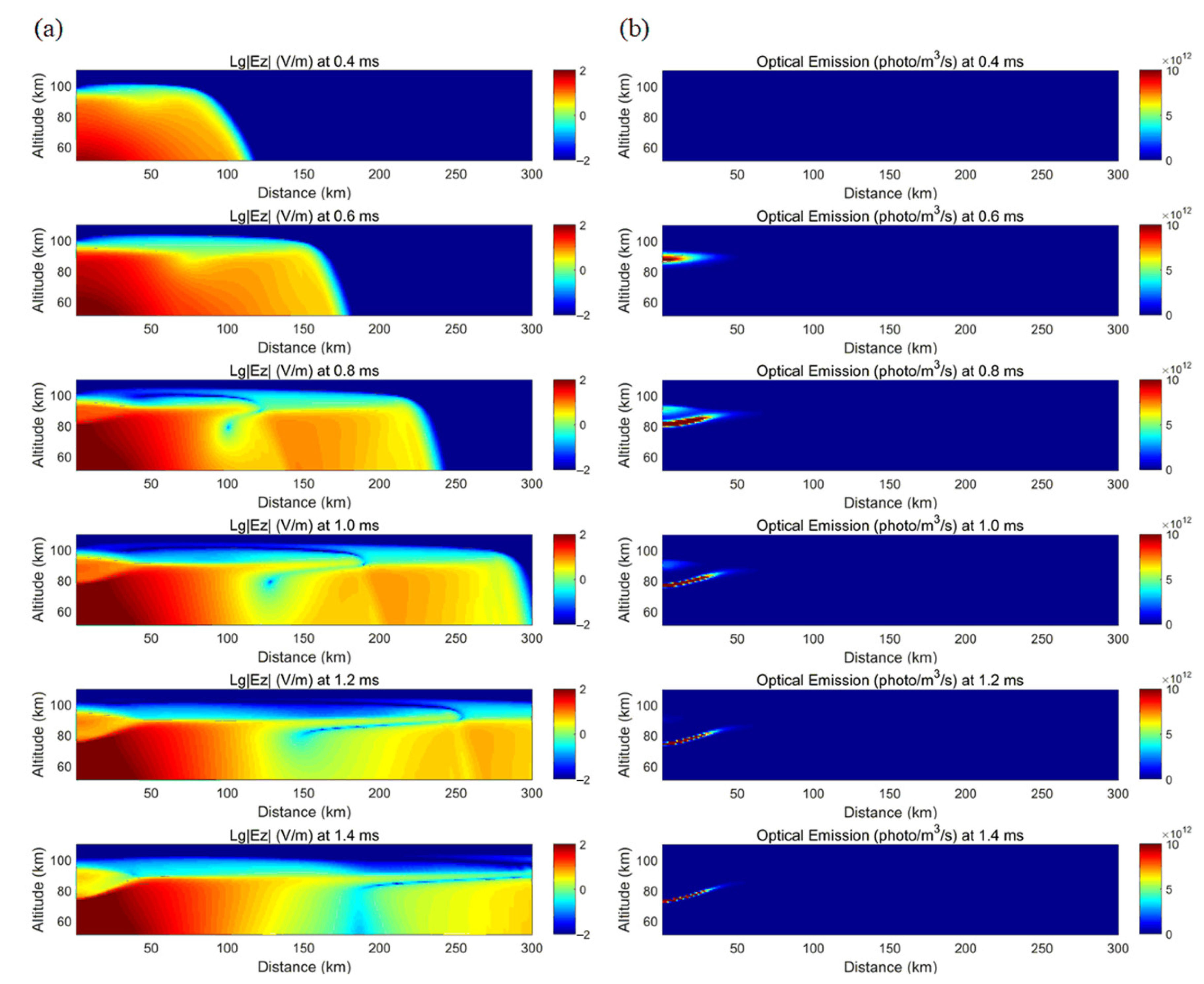
Figure 14 presents the temporal and spatial evolutions of the optical emissions of the sprite halos excited at mid-to-high altitudes at various moments after the discharge, but it neglects the influences of the gravity waves. Figure 14a shows the propagation and distribution of the spatial electric field generated by the selected lightning current of the simulated sprite halos. Because of the long duration and small steepness of the lightning current, the electrostatic field is primarily formed in space, and the radiation field part can be neglected. From the same figure, it can be seen that the electrostatic field’s distribution is still clustered below 100 km, and it is mainly distributed in an area that is horizontally 50 km within the vicinity of the lightning channel. The electric field’s distribution at 0.8 ms shows the occurrence of a relatively low value in the region right above the lightning channel, and this region continues to expand and extends downward with time. This is because the quasi-electrostatic field at the mid-to-high altitudes exceeds the threshold for air breakdown, thus triggering air breakdown. Consequently, the electron density within this region increases, which leads to the formation of a strong local electric field. In addition, the increased electron density in this region has a shielding effect on the region above, which lessens the amplitude of the electric field in this region.
Figure 14b shows the spatial distribution of the corresponding optical emissions of the sprite halos. As can be seen, the sprite halos originate at a height about 85 km above the lightning channel, and due to the symmetry of the 2D cylindrical coordinate model, the maximum horizontal scale can achieve 80 km in the simulation. The optical emission zone is pancake-shaped and exhibits a downward developing trend with time, which is consistent with the statistical characteristics of the actual observations.
Figure 15 shows the temporal and spatial distributions of the electric field and the optical emissions of the halos after considering perturbations (A = 40%) of the atmospheric density caused by the gravity wave. Compared with Figure 14, the distribution of the electric field in the region above the lightning channel is significantly affected by the gravity waves, while in the other regions the effect of the gravity waves is hardly noticeable. This analysis indicates that because the electrostatic field decays rapidly with distance, the amplitude of the electric field in the farther regions is insufficient and cannot cause air breakdown. As such, the effect of the gravity wave on the neutral air density fails to manifest itself in the farther regions. As can be seen in Figure 15b, the halos luminous zone contains obvious distortions and the shape of the optical emissions also becomes more sophisticated with time. The primary distortion region is located within 30 km of the lightning channel, which is also the region with the most recognizable electric field disturbance.
Figure 16 shows the effects of the different gravity wave disturbance amplitudes on the electric field and the optical emissions of the halos as an example (at 0.8 ms after the discharge). The spatial distributions of the electric field and the optical emissions of the halos under different gravity wave disturbances, in terms of its amplitude from 0 to 40%, are presented. It can be seen that as the amplitude of the gravity wave disturbance increases, the spatial distribution of the electric field at mid-to-high altitudes and the halos optical emission zone are more significantly affected.
5. Conclusions and Discussion
In this study, a tropospheric mid-to-high altitude electromagnetic radiation model was developed based on the 2D FDTD algorithm. By selecting appropriate lightning excitation sources, two classical transient luminous events (TLEs), i.e., ELVEs and halos, were simulated. The accuracy of the simulation model was verified through comparisons with the results reported in the relevant literature. The characteristics of the distributions of the spatial electric field and the optical emissions of these two phenomena were discussed separately using this model and considering the gravity wave perturbations at mid-to-high altitudes. The simulation results indicate that gravity waves affect the morphological development of both ELVEs and halos. The main conclusions are summarized as follows:
(1) The 2D electromagnetic pulse (EMP), established while considering the gravity wave disturbance, can accurately simulate the development of ELVEs and halos using the FDTD method. Because of the symmetry of the concentric gravity waves (CGWs), the accuracy of the test results of the 2D model established in this paper are consistent with that of the 3D model.
(2) When the electric field that generates the ELVEs develops upward to an altitude of 100 km, obvious downward reflection occurs. The optical emissions of the ELVEs propagate farther with a gradually diminishing light intensity. The total duration is about 1 ms, and the concentrated luminous zones are between 85 and 100 km. Because the radiation field is a manifestation of the change in the electric current, the rising and falling edges of the lightning current separately excite two radiation fields with various intensities, corresponding to two ELVEs luminous zones in which the inner optical emission field corresponds to the falling edge electric field, which has a modest steepness and a weaker light intensity. When including the perturbations of the neutral air density caused by CGWs, the electric field exhibits an obvious sparse and dense ripple pattern at altitudes of 90 to 100 km, and this mainly occurs during the electric field’s decline period, with a shallow steepness. The alternating distance of the variations in the sparse and dense patterns is about 40 km, which corresponds to the horizontal wavelength of the electric field. The inner optical emission field is obviously deformed and is even split into multiple luminous zones. As the amplitude of the gravity wave disturbance increases, the spatial distribution of the electric field at mid-to-high altitudes is perturbed more significantly, and similarly, the changes in the ELVEs luminous pattern are more pronounced.
(3) The lightning current that generates sprite halos has a long duration and a small steepness. Its generated electrostatic field is clustered below 100 km and is mainly distributed in an area that is horizontally 50 km within the vicinity of the lightning channel. At 0.8 ms, the region right above the lightning channel forms a strong local electric field due to the small scale air breakdown, in which the increased electron density has a shielding effect on the region above and lessens the amplitude of the electric field in this region. In the optical emission field, the sprite halo’s luminous zone is pancake-shaped, and it originates at an altitude of 85 km along with a downward developing trend with time. The disturbance of the sprite halos by the CGWs primarily occurs at about 80 to 100 km, i.e., directly above the lightning channel, where their regions with clear alternating strengths exist. Because the electrostatic field decays rapidly with distance, the amplitude of the electric field in the farther regions is insufficient and cannot cause air breakdown; therefore, the effect of the gravity waves on the neutral air density fails to manifest itself in the farther regions. The halo’s luminous zone contains obvious distortions, and its primary deformed region is located within 30 km of the lightning channel, which is also the region with the most recognizable electric field disturbance. Like ELVEs, as the amplitude of the gravity wave disturbance increases, the disturbance of the electric field becomes more significant at mid-to-high altitudes, and the changes in the halo’s luminous pattern become more pronounced.
Author Contributions
Conceptualization, Y.W. and C.W.; methodology, C.W. and Q.Z.; software, J.Z. and C.W.; validation, Y.W. and Q.Z.; formal analysis, Y.W. and J.Q.; data curation, J.Z. and J.Q.; writing—original draft preparation, C.W.; writing—review and editing, Y.W. and J.Z.; visualization, C.W. All authors have read and agreed to the published version of the manuscript.
Funding
This research was jointly funded by the National Key R&D Program of China, grant number 2017YFC1501505, and the National Natural Science Foundations of China, grant number 41775006.
Institutional Review Board Statement
Not applicable.
Informed Consent Statement
Not applicable.
Data Availability Statement
Not applicable.
Acknowledgments
Special thanks to the reviewers for their valuable comments.
Conflicts of Interest
The authors declare no conflict of interest. The funders had no role in the design of the study; in the collection, analyses, or interpretation of data; in the writing of the manuscript; or in the decision to publish the results.
References
- Qie, X.S.; Lv, D.R.; Bian, J.C.; Yang, J. Transient Luminous Events (TLEs) at high altitudes above thunderstorms and their possible effects. Adv. Earth Sci. 2009, 24, 286–296. [Google Scholar] [CrossRef]
- Zhang, J.B.; Zhang, Q.L.; Guo, X.F.; Hou, W.H.; Gao, H.Y. Simulated impacts of atmospheric gravity waves on the initiation and optical emissions of sprite halos in the mesosphere. Sci. China Earth Sci. 2019, 62, 631–642. [Google Scholar] [CrossRef]
- Franz, R.C.; Nemzek, R.J.; Winckler, J.R. Television image of a large upward electric discharge above a thunderstorm system. Science 1990, 249, 48–51. [Google Scholar] [CrossRef]
- Wu, M.L.; Xu, J.Y.; Ma, R.P. The simulation study of spherics and red sprite phenomenon produced by lightning. Acta Phys. Sin. 2006, 55, 5007–5013. [Google Scholar] [CrossRef]
- Rycroft, M.J.; Harrison, R.G.; Nicoll, K.A.; Mareev, E.A. An overview of earth’s global electric circuit and atmospheric conductivity. Space Sci. Rev. 2008, 137, 83–105. [Google Scholar] [CrossRef]
- Yang, J.; Qie, X.S.; Zhang, G.S.; Zhao, Y.; Zhang, T. Red sprites over thunderstorms in the coast of Shandong Province, China. Chin. Sci. Bull. 2008, 53, 482–488. (In Chinese) [Google Scholar] [CrossRef] [Green Version]
- Zhang, Q.L.; Tian, Y.; Lu, G.P. Effects of the nonlinear atmospheric electric parameters at the high altitudes on the propagation of lightning return stroke electromagnetic field. Acta Meteorol. Sin. 2014, 72, 805–814. [Google Scholar] [CrossRef]
- Pasko, V.P.; Inan, U.S.; Bell, T.F. Sprites as evidence of vertical gravity wave structures above mesoscale thunderstorms. Geophys. Res. Lett. 1997, 24, 1735–1738. [Google Scholar] [CrossRef]
- Yang, J.; Qie, X.S.; Feng, G.L. Characteristics of one sprite-producing summer thunderstorm. Atmos. Res. 2013, 127, 90–115. [Google Scholar] [CrossRef]
- Wen, Y.; Zhang, Q.L.; Xu, J.Y.; Li, Q.Z.; Gao, H.Y. Propagation characteristics of mesospheric concentric gravity waves excited by a thunderstorm. Chin. J. Geophys. 2019, 62, 1218–1229. [Google Scholar] [CrossRef]
- Taranenko, Y.N.; Inan, U.S.; Bell, T.F. Interaction with the lower ionosphere of electromagnetic pulses from lightning: Heating, attachment, and ionization. Geophys. Res. Lett. 1993, 20, 1539–1542. [Google Scholar] [CrossRef]
- Ren, H.; Tian, Y.; Lu, G.P.; Zhang, Y.F.; Fan, Y.F.; Jiang, R.B.; Liu, M.Y.; Li, D.S.; Qie, X.S. Examining the influence of current waveform on the lightning electromagnetic field at the altitude of halo formation. J. Atmos. Terr. Phys. 2019, 189, 114–122. [Google Scholar] [CrossRef]
- Pérez-Invernón, F.J.; Luque, A.; Gordillo-Vázquez, F.J.; Sato, M.; Ushio, T.; Adachi, T.; Chen, A.B. Spectroscopic diagnostic of halos and elves detected from space-based photometers. J. Geophys. Res. Atmos. 2019, 27, 12917–12941. [Google Scholar] [CrossRef]
- Rowland, H.L. Theories and simulations of elves, sprites and blue jets. J. Atmos. Terr. Phys. 1998, 60, 831–844. [Google Scholar] [CrossRef]
- Heavner, M.; Sentman, D.D.; Moudry, D.R.; Wescott, E.; Siefring, C.L.; Morrill, J.; Bucsela, E. Sprites, Blue Jets, and Elves: Optical evidence of energy transport across the stratopause. Am. Geophys. Union 2013. [Google Scholar] [CrossRef] [Green Version]
- Wen, Y.; Zhang, Q.L.; Gao, H.Y.; Xu, J.Y.; Li, Q.Z. A Case Study of the stratospheric and mesospheric concentric gravity waves excited by thunderstorm in northern China. Atmosphere 2018, 9, 489. [Google Scholar] [CrossRef] [Green Version]
- Vadas, S.; Yue, J.; Nakamura, T. Mesospheric concentric gravity waves generated by multiple convective storms over the North American Great Plain. J. Geophys. Res. Atmos. 2012, 117, D7. [Google Scholar] [CrossRef]
- Vargas, F.; Swenson, G.; Liu, A.; Pautet, D. Evidence of the excitation of a ring-like gravity wave in the mesosphere over the Andes Lidar Observatory. J. Geophys. Res. Atmos. 2016, 121, 8896–8912. [Google Scholar] [CrossRef]
- Xu, J.Y.; Li, Q.Z.; Yue, J.; Hoffmann, L.; Straka, W.C.; Wang, C.M.; Liu, M.H.; Yuan, W.; Han, S.; Miller, S.D.; et al. Concentric gravity waves over northern China observed by an airglow imager network and satellites. J. Geophys. Res. Atmos. 2015, 120, 11058–11078. [Google Scholar] [CrossRef] [Green Version]
- Lai, C.; Li, W.; Xu, J.Y.; Liu, X.; Yuan, W.; Yue, J.; Li, Q.Z. Extraction of quasi-monochromatic gravity waves from an airglow imager network. Atmosphere 2020, 11, 615. [Google Scholar] [CrossRef]
- Siefring, C.L.; Morrill, J.S.; Sentman, D.D.; Heavner, M.J. Simultaneous near-infrared and visible observations of sprites and acoustic-gravity waves during the EXL98 campaign. J. Geophys. Res. Space Phys. 2010, 115, A00E57. [Google Scholar] [CrossRef] [Green Version]
- Gong, J.; Yue, J.; Wu, D.L. Global survey of concentric gravity waves in AIRS images and ECMWF analysis. J. Geophys. Res. Atmos. 2015, 120, 2210–2228. [Google Scholar] [CrossRef] [Green Version]
- Yue, J.; Miller, S.D.; Hoffmann, L.; Straka, W.C. Stratospheric and mesospheric concentric gravity waves over tropical cyclone Mahasen: Joint AIRS and VIIRS satellite observations. J. Atmos. Terr. Phys. 2014, 119, 83–90. [Google Scholar] [CrossRef]
- Gong, S.H.; Yang, G.T.; Xu, J.Y.; Liu, X.; Li, Q.Z. Gravity wave propagation from the stratosphere into the mesosphere studied with Lidar, Meteor Radar, and TIMED/SABER. Atmosphere 2019, 10, 81. [Google Scholar] [CrossRef] [Green Version]
- Yue, J.; Lyons, W.A. Structured elves: Modulation by convectively generated gravity waves. Geophys. Res. Lett. 2015, 42, 1004–1011. [Google Scholar] [CrossRef]
- Marshall, R.A.; Yue, J.; Lyons, W.A. Numerical simulation of an elve modulated by a gravity wave. Geophys. Res. Lett. 2015, 42, 6120–6127. [Google Scholar] [CrossRef]
- Yee, K.S. Numerical solution of initial boundary value problems involving maxwell’s equations in isotropic media. IEEE Trans. Antennas Propag. 1966, 14, 302–307. [Google Scholar] [CrossRef] [Green Version]
- Hu, W.Y. A Numerical Model of Lightning-Generated EM Waves and Remote Sensing Applications; Duke University: Durham, NC, USA, 2005. [Google Scholar]
- Pasko, V.P. Dynamic Coupling of Quasi-Electrostatic Thundercloud Fields to the Mesosphere and Lower Ionosphere: Sprites and Jets. Ph.D. Thesis, Stanford University, Stanford, CA, USA, 1996. [Google Scholar]
- Dejnakarintra, M.; Park, C.G. Lightning-induced electric fields in the ionosphere. J. Geophys. Res. Atmos. 1974, 79, 1903–1910. [Google Scholar] [CrossRef]
- Hegerberg, R.; Reid, I.D. Electron drift velocities in air. Aust. J. Phys. 1980, 33, 227–238. Available online: https://www.publish.csiro.au/PH/pdf/PH800227a (accessed on 25 December 1979). [CrossRef] [Green Version]
- Han, F.; Cummer, S.A. Midlatitude nighttime D region ionosphere variability on hourly to monthly time scales. J. Geophys. Res. Atmos. 2010, 115, A09323. [Google Scholar] [CrossRef]
- Papadopoulos, K.; Milikh, G.; Gurevich, A.; Drobot, A.; Shanny, R. Ionization rates for atmospheric and ionospheric breakdown. J. Geophys. Res. Space Phys. 1993, 98, 17593–17596. [Google Scholar] [CrossRef]
- Taranenko, Y.N.; Inan, U.S.; Bell, T.F. The interaction with the lower ionosphere of electromagnetic pulses from lightning: Excitation of optical emissions. Geophys. Res. Lett. 1993, 20, 2675–2678. [Google Scholar] [CrossRef]
- Sipler, D.P.; Biondi, M.A. Measurements of O(1D) quenching rates in the F region. J. Geophys. Res. Space Phys. 1972, 77, 6202–6212. [Google Scholar] [CrossRef]
- Qin, J.Q.; Pasko, V.P.; McHarg, M.G.; Stenbaek-Nielsen, H.C. Plasma irregularities in the D-region ionosphere in association with sprite streamer initiation. Nat. Commun. 2014, 5, 536–538. [Google Scholar] [CrossRef] [Green Version]
- Rowland, H.L.; Fernsler, R.F.; Bernhardt, P.A. Breakdown of the neutral atmosphere in the D region due to lightning driven electromagnetic pulses. J. Geophys. Res. Space Phys. 1996, 101, 7935–7946. [Google Scholar] [CrossRef]
- Liu, N.; Boggs, L.D.; Cummer, S.A. Observation-constrained modeling of the ionospheric impact of negative sprites. Geophys. Res. Lett. 2016, 43, 2365–2373. [Google Scholar] [CrossRef] [Green Version]
- Barrington-Leigh, C.P.; Inan, U.S.; Stanley, M. Identification of sprites and elves with intensified video and broadband array photometry. J. Geophys. Res. Space Phys. 2001, 106, 1741–1750. [Google Scholar] [CrossRef]
Figure 1.
Two-dimensional FDTD-EMP algorithm model.

Figure 2.
Discretization of electromagnetic field in a two-dimensional cylindrical coordinate system.
Figure 2.
Discretization of electromagnetic field in a two-dimensional cylindrical coordinate system.

Figure 3.
Variation of electron density with altitude.

Figure 4.
Ionization coefficient and absorption coefficient.

Figure 5.
Neutral air density.

Figure 6.
Electron mobility.

Figure 7.
Perturbation of gravity waves to air density.

Figure 8.
The comparison of model calculation results in this article (left) and CP Barrington-Leigh [39] results (right).
Figure 8.
The comparison of model calculation results in this article (left) and CP Barrington-Leigh [39] results (right).

Figure 9.
Simulation of ELVEs lightning current waveform (a) and the amount of transferred charges (b).
Figure 9.
Simulation of ELVEs lightning current waveform (a) and the amount of transferred charges (b).

Figure 10.
Spatial and temporal distribution of the electric field (a) and the optical emissions of the ELVEs (b) without gravity wave disturbance.
Figure 10.
Spatial and temporal distribution of the electric field (a) and the optical emissions of the ELVEs (b) without gravity wave disturbance.

Figure 11.
Spatial and temporal distribution of the electric field (a) and the optical emissions of the ELVEs (b) after the gravity wave disturbance (with a disturbance amplitude of A = 40%).
Figure 11.
Spatial and temporal distribution of the electric field (a) and the optical emissions of the ELVEs (b) after the gravity wave disturbance (with a disturbance amplitude of A = 40%).

Figure 12.
The spatial distributions of the spatial electric field (a) and the optical emissions of the ELVEs (b) under different gravity wave disturbances in the range of 0 to 40% (at 0.8 ms after the discharge).
Figure 12.
The spatial distributions of the spatial electric field (a) and the optical emissions of the ELVEs (b) under different gravity wave disturbances in the range of 0 to 40% (at 0.8 ms after the discharge).

Figure 13.
Simulation of sprite halos lightning current waveform (a) and the amount of transferred charge (b).
Figure 13.
Simulation of sprite halos lightning current waveform (a) and the amount of transferred charge (b).

Figure 14.
Spatial and temporal distribution of the electric field (a) and the optical emissions of the halos (b) without gravity wave disturbance.
Figure 14.
Spatial and temporal distribution of the electric field (a) and the optical emissions of the halos (b) without gravity wave disturbance.

Figure 15.
Spatial and temporal distribution of the electric field (a) and the optical emissions of the halos (b) after the gravity wave disturbance (with a disturbance amplitude of A = 40%).
Figure 15.
Spatial and temporal distribution of the electric field (a) and the optical emissions of the halos (b) after the gravity wave disturbance (with a disturbance amplitude of A = 40%).

Figure 16.
The spatial distributions of the spatial electric field (a) and the optical emissions of the halos (b) under different gravity wave disturbances in the range of 0 to 40% (at 0.8 ms after the discharge).
Figure 16.
The spatial distributions of the spatial electric field (a) and the optical emissions of the halos (b) under different gravity wave disturbances in the range of 0 to 40% (at 0.8 ms after the discharge).

Publisher’s Note: MDPI stays neutral with regard to jurisdictional claims in published maps and institutional affiliations. |
© 2021 by the authors. Licensee MDPI, Basel, Switzerland. This article is an open access article distributed under the terms and conditions of the Creative Commons Attribution (CC BY) license (https://creativecommons.org/licenses/by/4.0/).
Share and Cite
MDPI and ACS Style
Wang, C.; Wen, Y.; Zhang, J.; Zhang, Q.; Qiu, J. The Modulation Effect on the ELVEs and Sprite Halos by Concentric Gravity Waves Based on the Electromagnetic Pulse Coupled Model. Atmosphere 2021, 12, 617. https://doi.org/10.3390/atmos12050617
AMA Style
Wang C, Wen Y, Zhang J, Zhang Q, Qiu J. The Modulation Effect on the ELVEs and Sprite Halos by Concentric Gravity Waves Based on the Electromagnetic Pulse Coupled Model. Atmosphere. 2021; 12(5):617. https://doi.org/10.3390/atmos12050617
Chicago/Turabian StyleWang, Chao, Ying Wen, Jinbo Zhang, Qilin Zhang, and Juwei Qiu. 2021. "The Modulation Effect on the ELVEs and Sprite Halos by Concentric Gravity Waves Based on the Electromagnetic Pulse Coupled Model" Atmosphere 12, no. 5: 617. https://doi.org/10.3390/atmos12050617
Note that from the first issue of 2016, this journal uses article numbers instead of page numbers. See further details here.