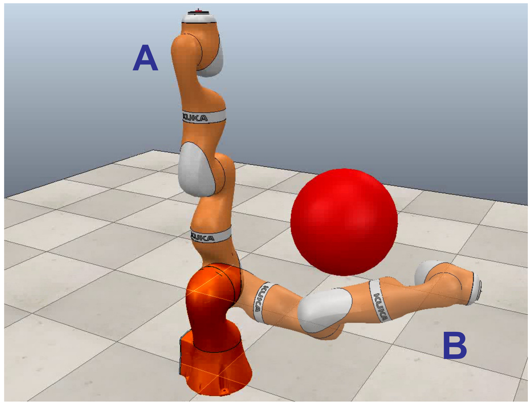
Figure 1.
Robot manipulator collision-free path planning problem.
Figure 1.
Robot manipulator collision-free path planning problem.
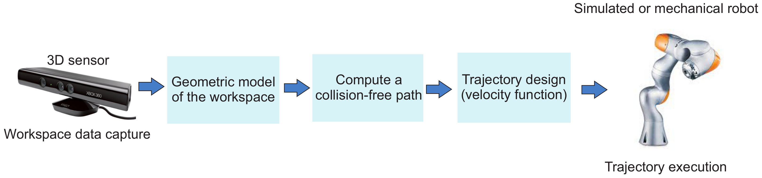
Figure 2.
System architecture of an autonomous manipulator.
Figure 2.
System architecture of an autonomous manipulator.
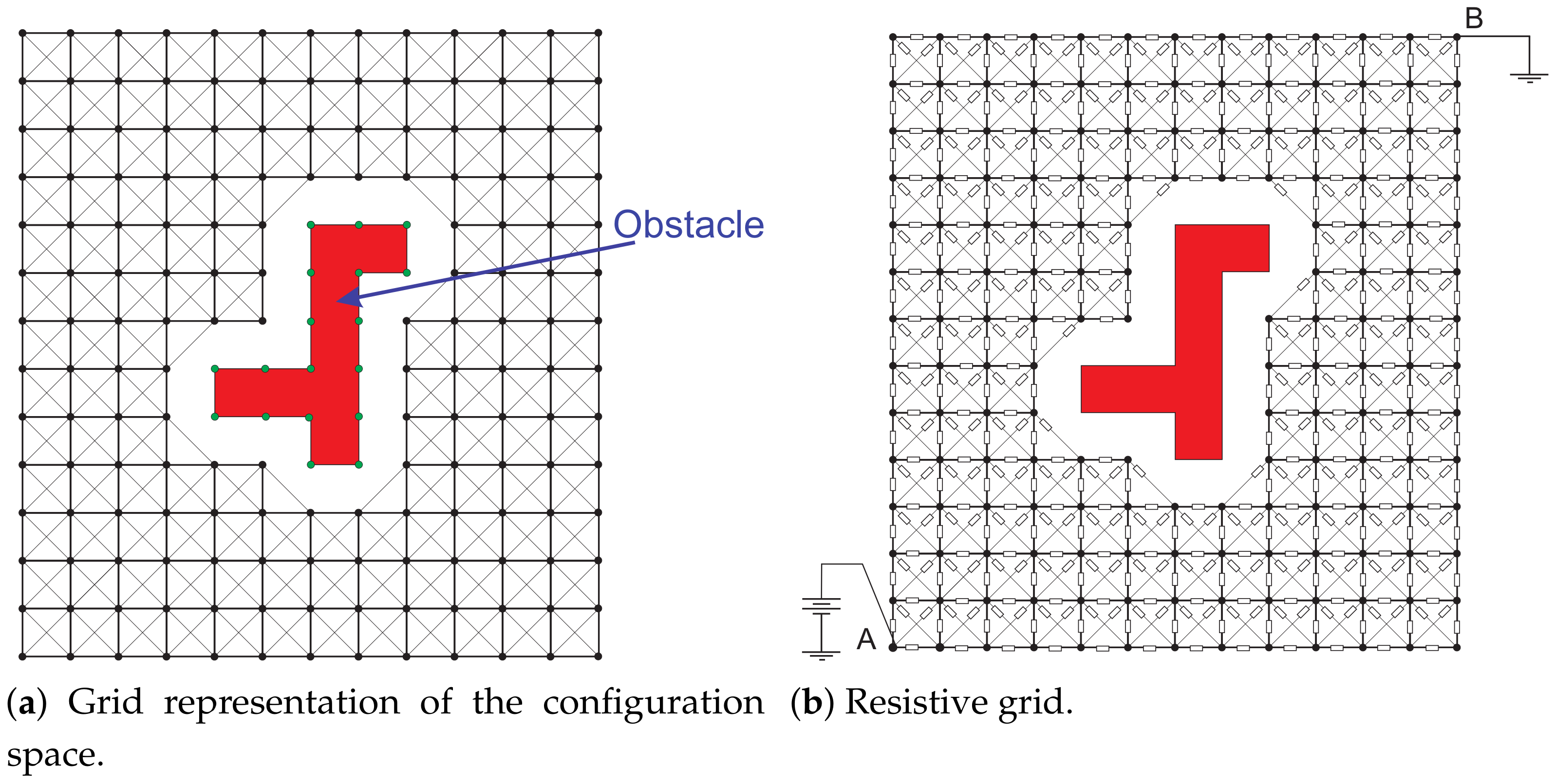
Figure 3.
Two-dimensional resistive grid representation of the configuration space.
Figure 3.
Two-dimensional resistive grid representation of the configuration space.
Figure 4.
Local current comparison representation.
Figure 4.
Local current comparison representation.
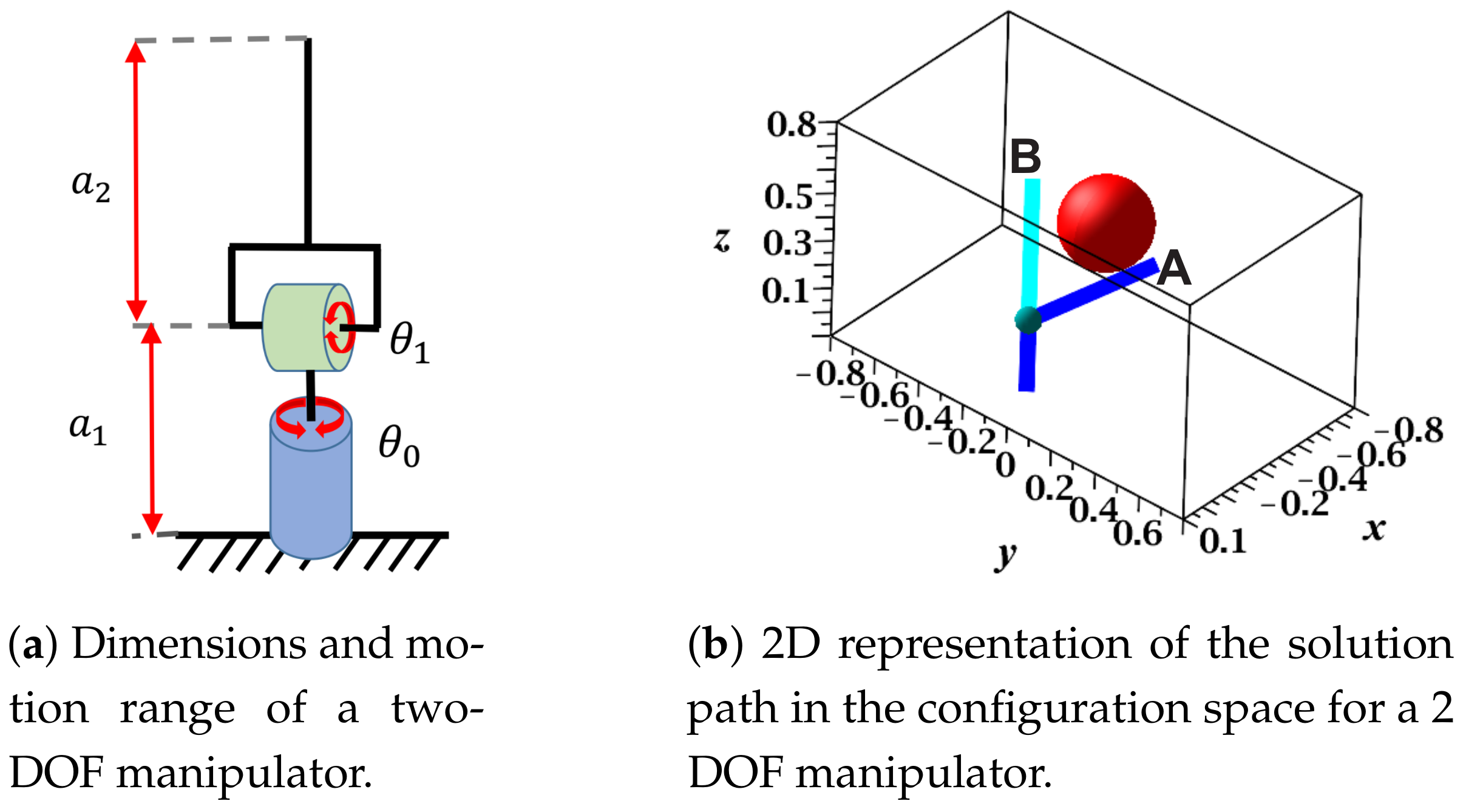
Figure 5.
Dimensions, motion range, and start–target configurations of a two-DOF manipulator.
Figure 5.
Dimensions, motion range, and start–target configurations of a two-DOF manipulator.
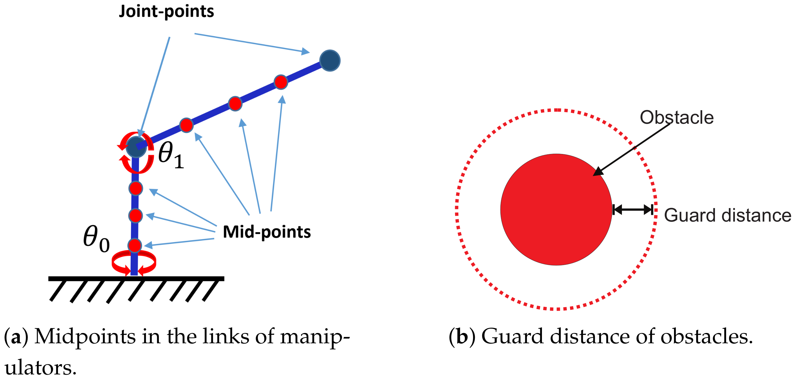
Figure 6.
Midpoints and guard distance of obstacles.
Figure 6.
Midpoints and guard distance of obstacles.
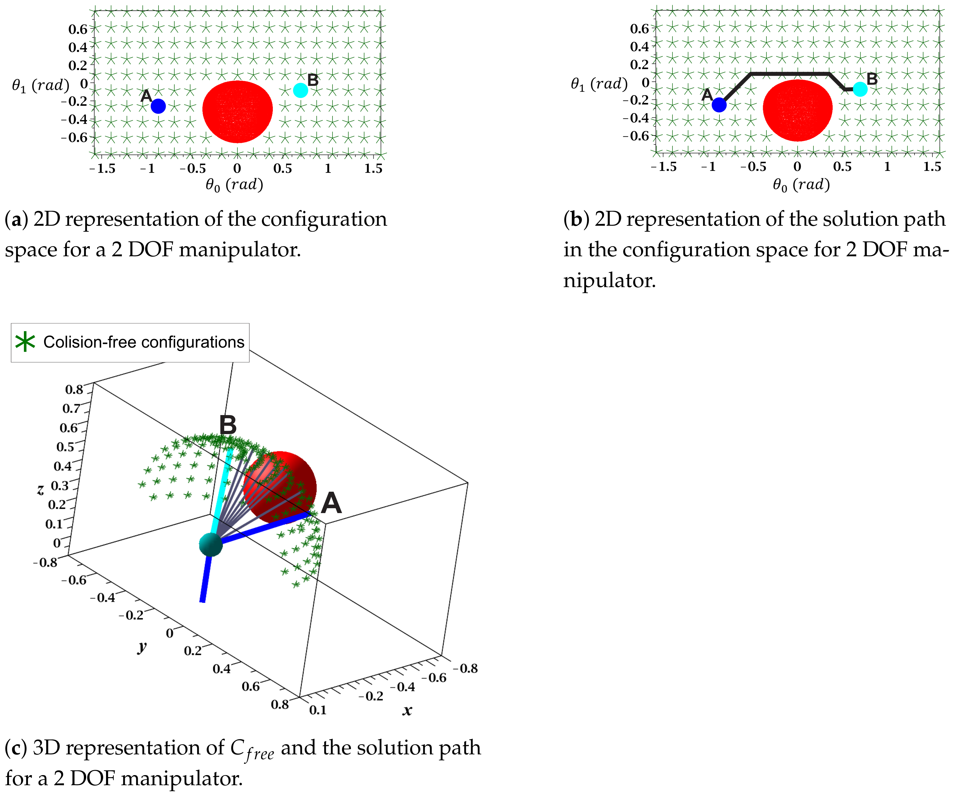
Figure 7.
Configuration space () for a 2 DOF manipulator.
Figure 7.
Configuration space () for a 2 DOF manipulator.
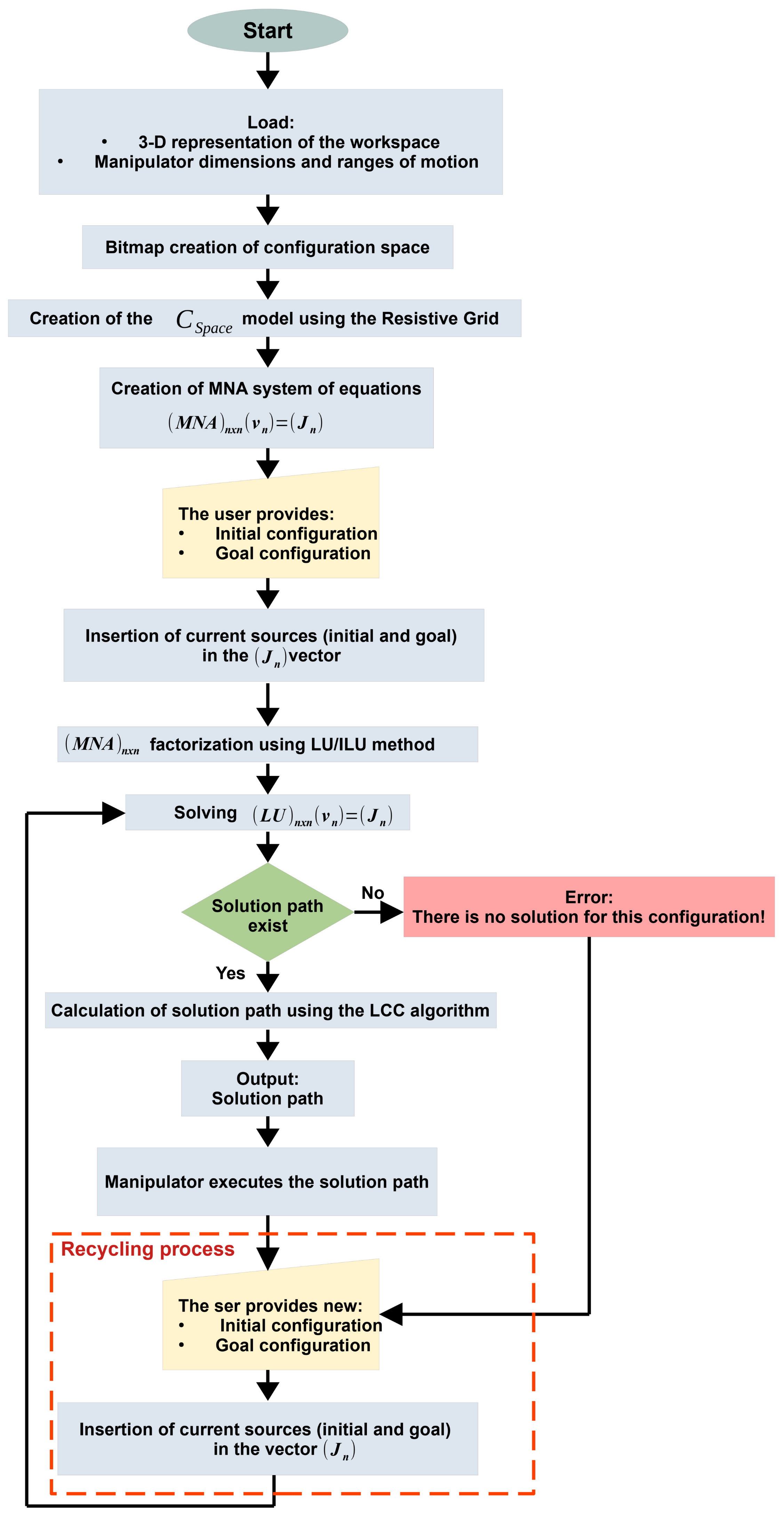
Figure 8.
Flowchart of multiple-query RGPM for high-DOF manipulators.
Figure 8.
Flowchart of multiple-query RGPM for high-DOF manipulators.
Figure 9.
Dimensions and motion range of a 3 DOF manipulator.
Figure 9.
Dimensions and motion range of a 3 DOF manipulator.
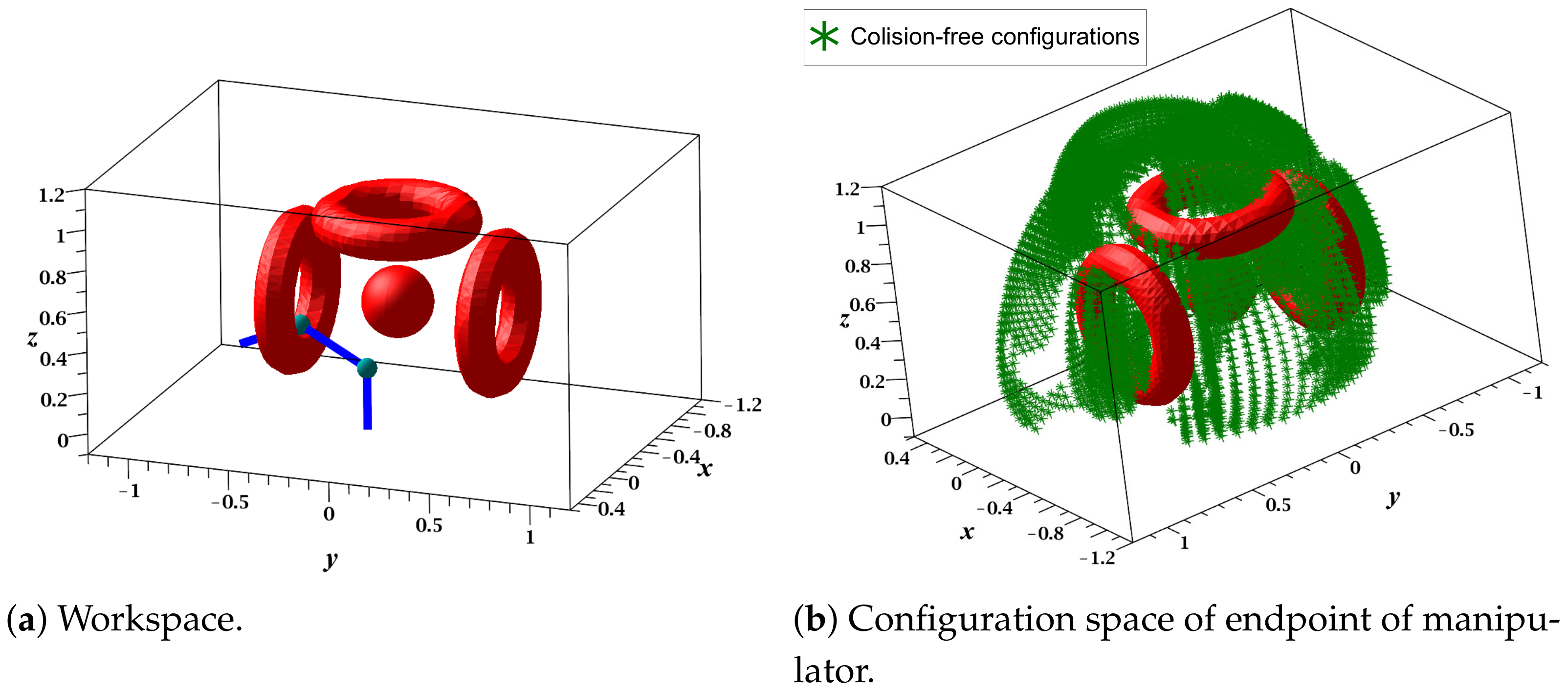
Figure 10.
Workspace and Configuration space (3 DOF manipulator).
Figure 10.
Workspace and Configuration space (3 DOF manipulator).
Figure 11.
A 3 DOF manipulator collision-free path of query 1 (sequence of configurations): .
Figure 11.
A 3 DOF manipulator collision-free path of query 1 (sequence of configurations): .
Figure 12.
Recycled collision-free paths of the 3 DOF manipulator.
Figure 12.
Recycled collision-free paths of the 3 DOF manipulator.
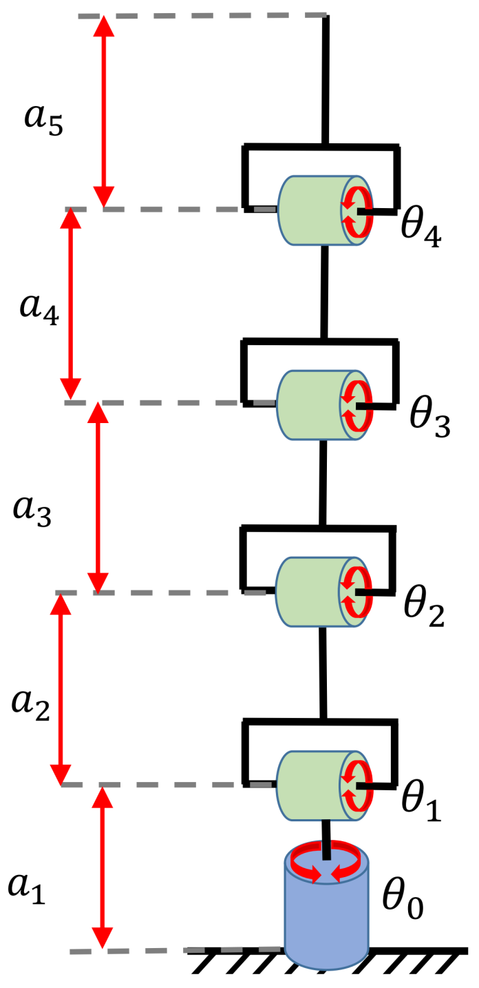
Figure 13.
Dimensions and motion range of the five DOF manipulator.
Figure 13.
Dimensions and motion range of the five DOF manipulator.
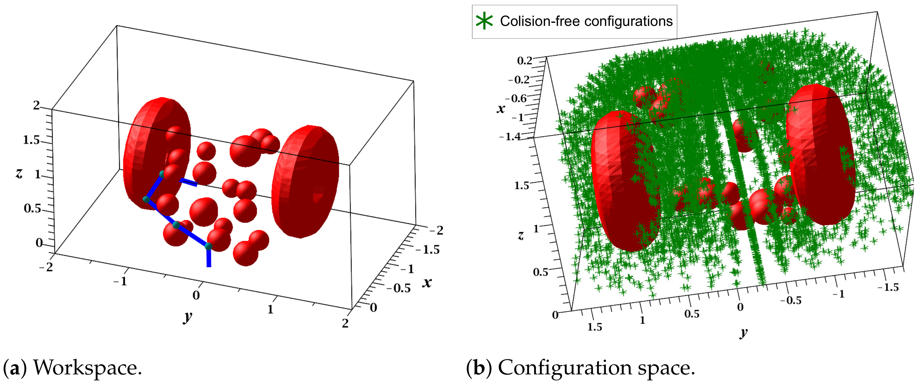
Figure 14.
Workspace and configuration space of the five-DOF manipulator.
Figure 14.
Workspace and configuration space of the five-DOF manipulator.
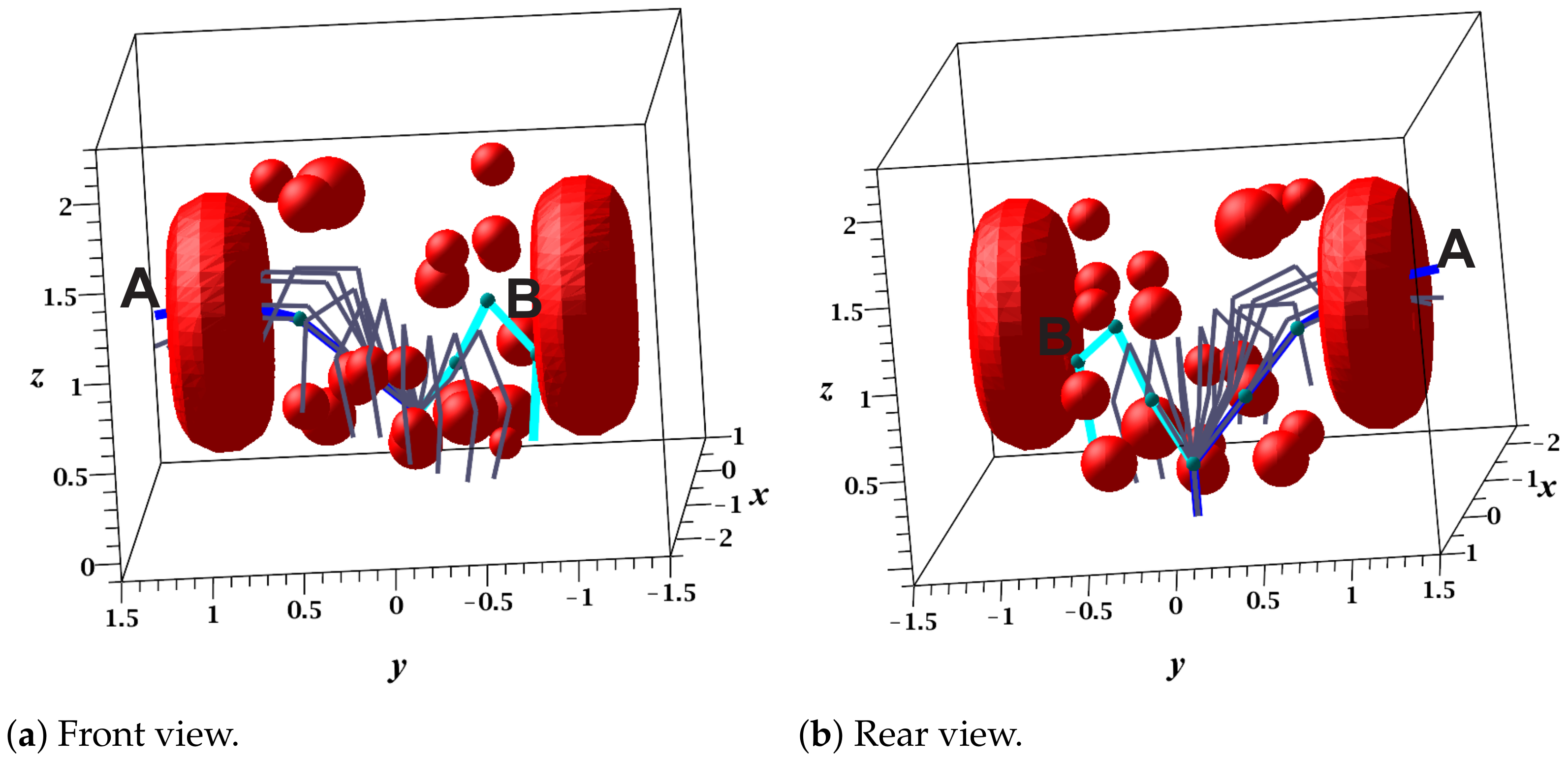
Figure 15.
The 5 DOF manipulator’s collision-free path (sequence of configurations). and .
Figure 15.
The 5 DOF manipulator’s collision-free path (sequence of configurations). and .
Figure 16.
Recycled collision-free paths of the five-DOF manipulator.
Figure 16.
Recycled collision-free paths of the five-DOF manipulator.
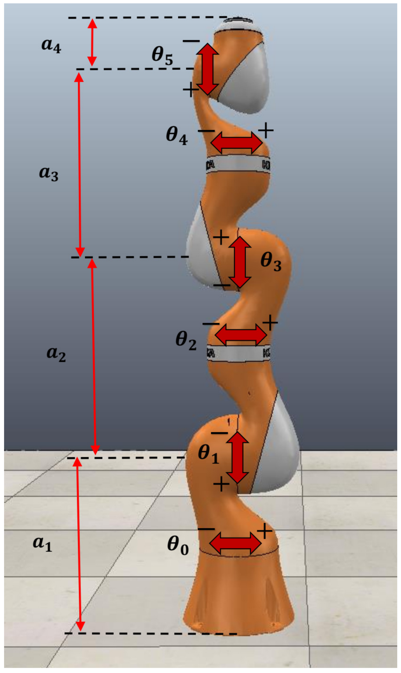
Figure 17.
Parameters of the KUKA LBR iiwa 14R820 robot manipulator.
Figure 17.
Parameters of the KUKA LBR iiwa 14R820 robot manipulator.
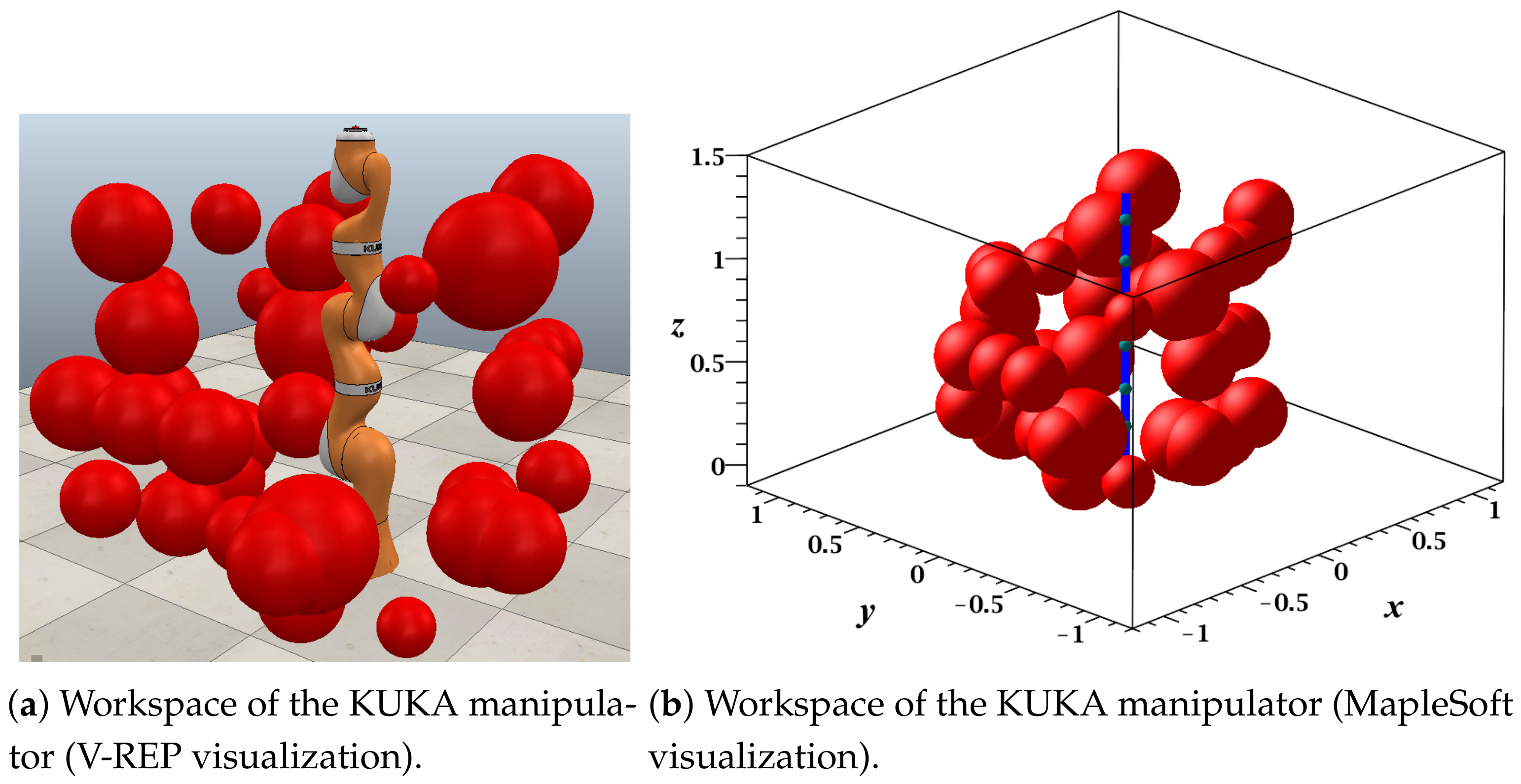
Figure 18.
Workspace and configuration space of the KUKA 6 DOF manipulator: Maple Soft and V-REP visualization.
Figure 18.
Workspace and configuration space of the KUKA 6 DOF manipulator: Maple Soft and V-REP visualization.
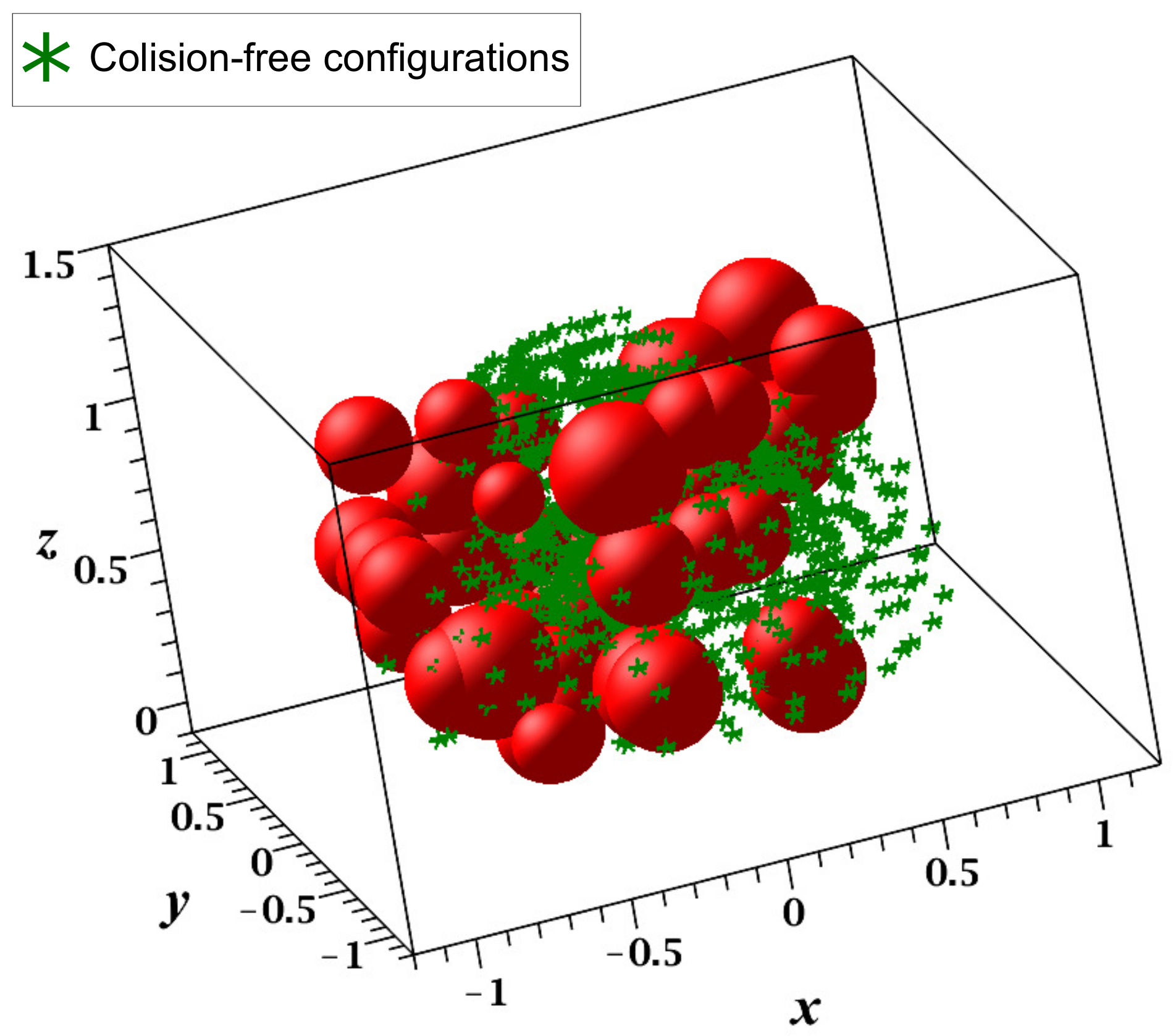
Figure 19.
Configuration space of the KUKA manipulator (MapleSoft visualization).
Figure 19.
Configuration space of the KUKA manipulator (MapleSoft visualization).
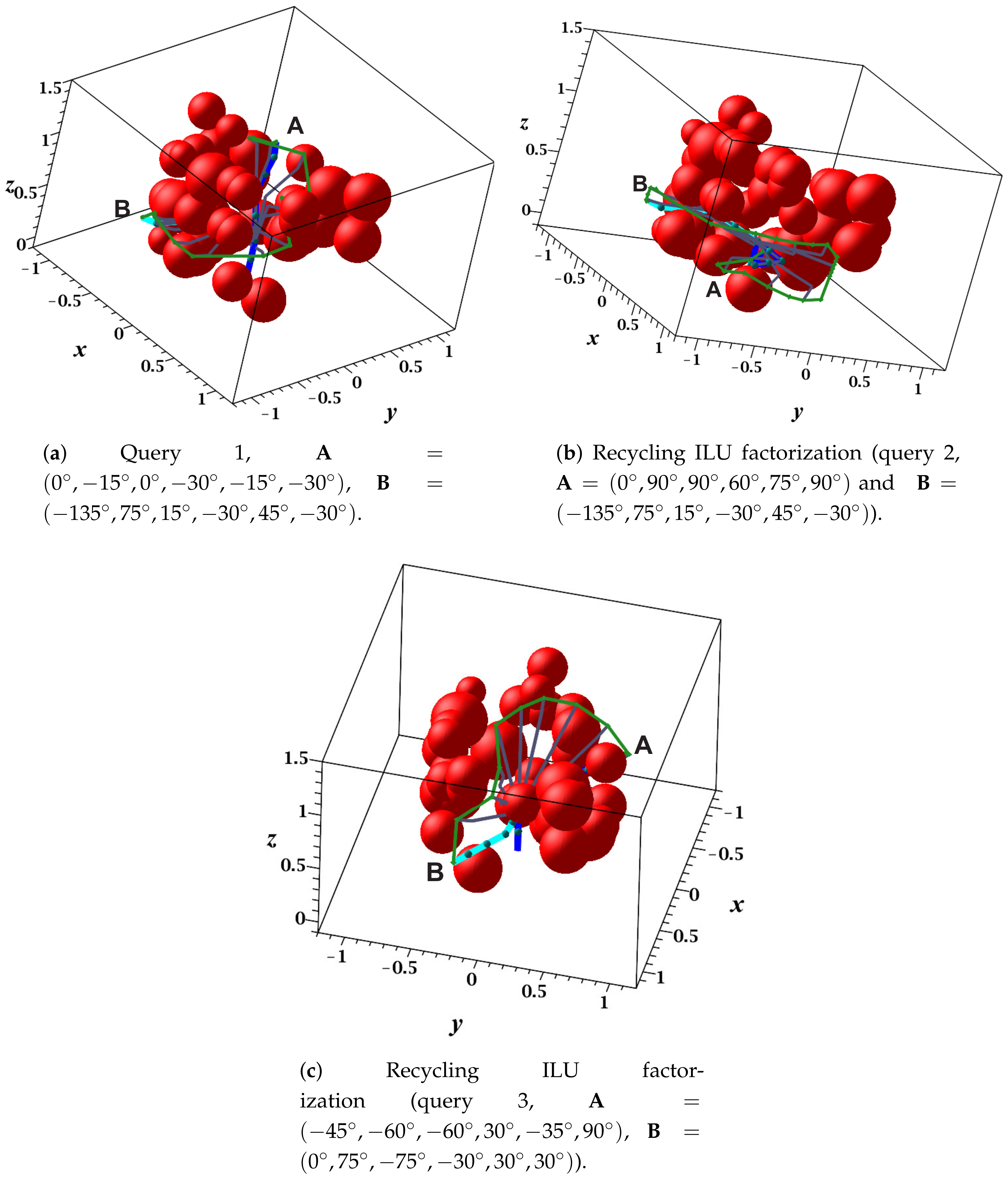
Figure 20.
Collision-free path for a KUKA manipulator: MapleSoft visualization.
Figure 20.
Collision-free path for a KUKA manipulator: MapleSoft visualization.
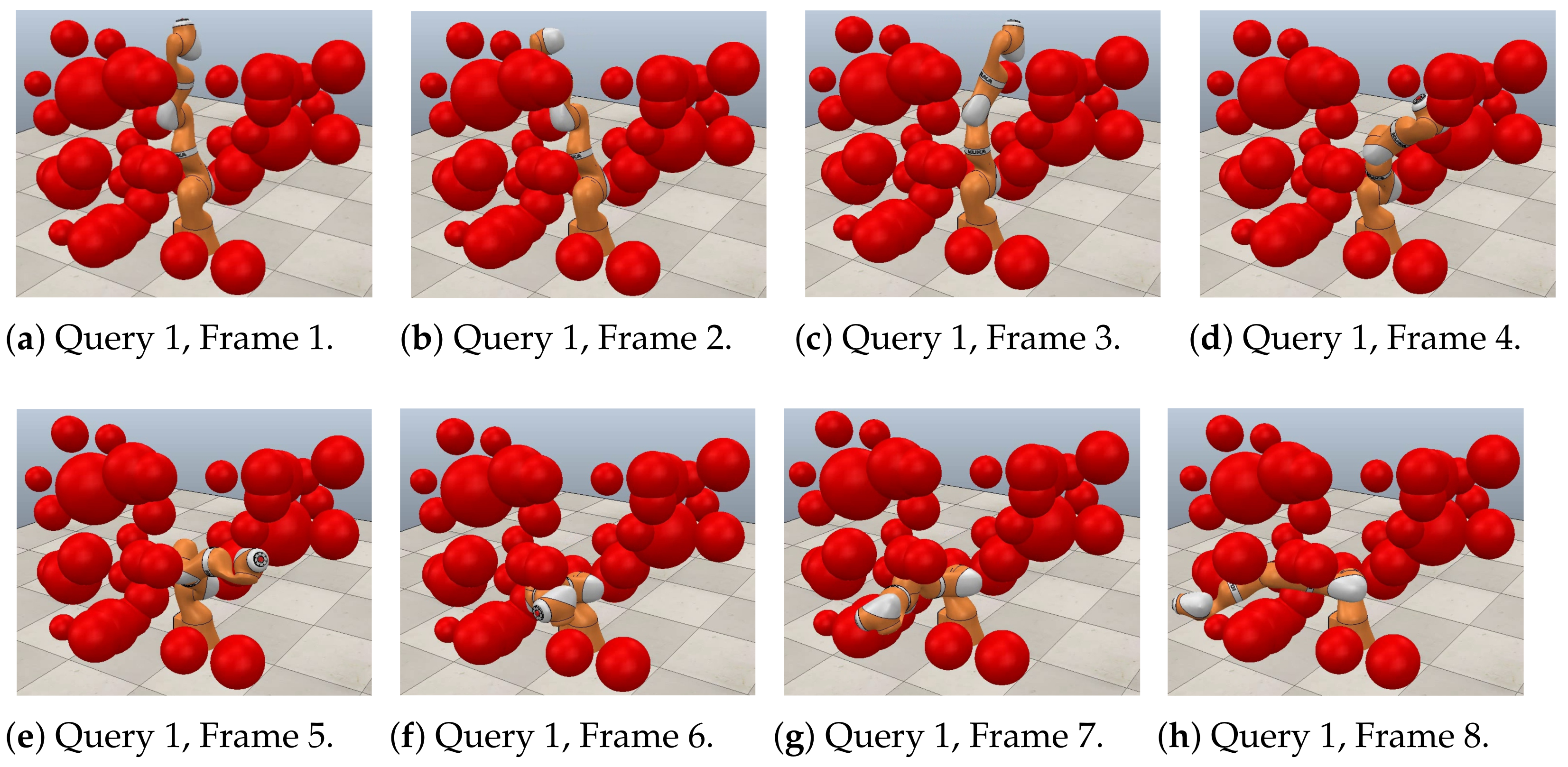
Figure 21.
Collision-free path for a KUKA manipulator. Query 1, and .
Figure 21.
Collision-free path for a KUKA manipulator. Query 1, and .
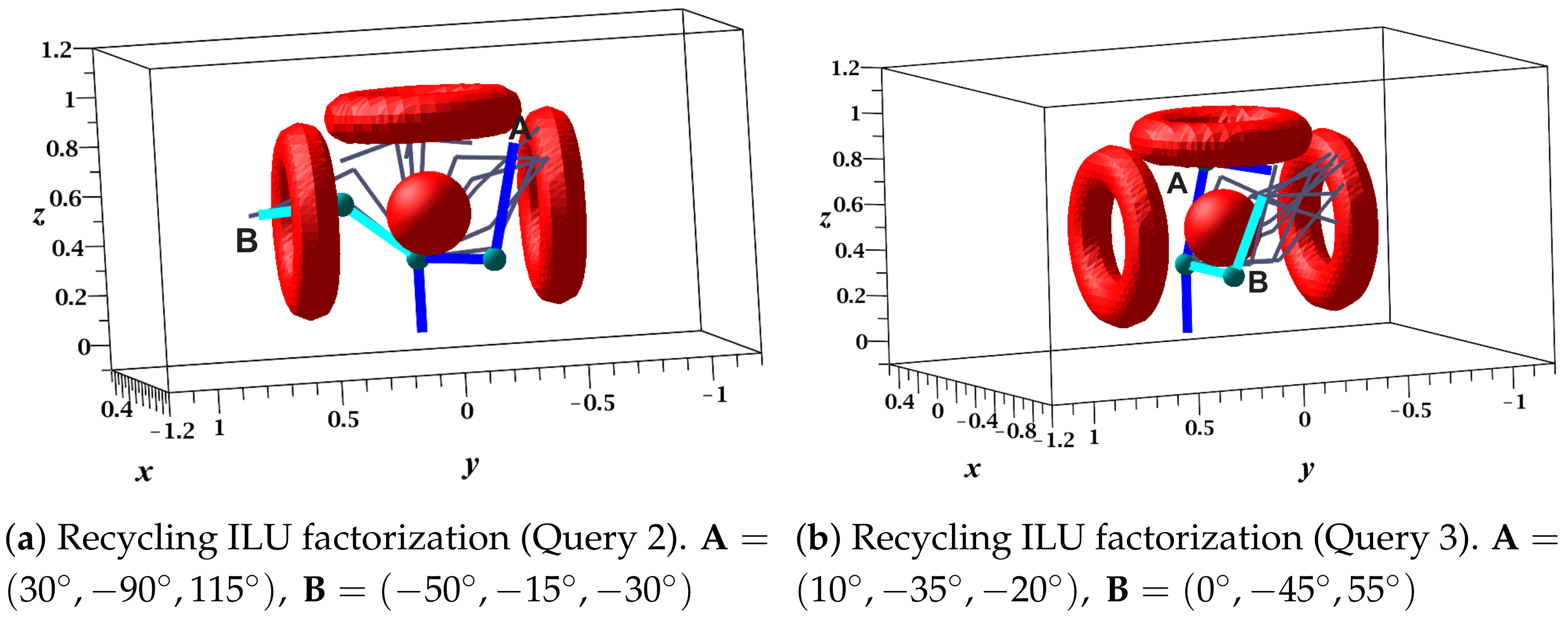
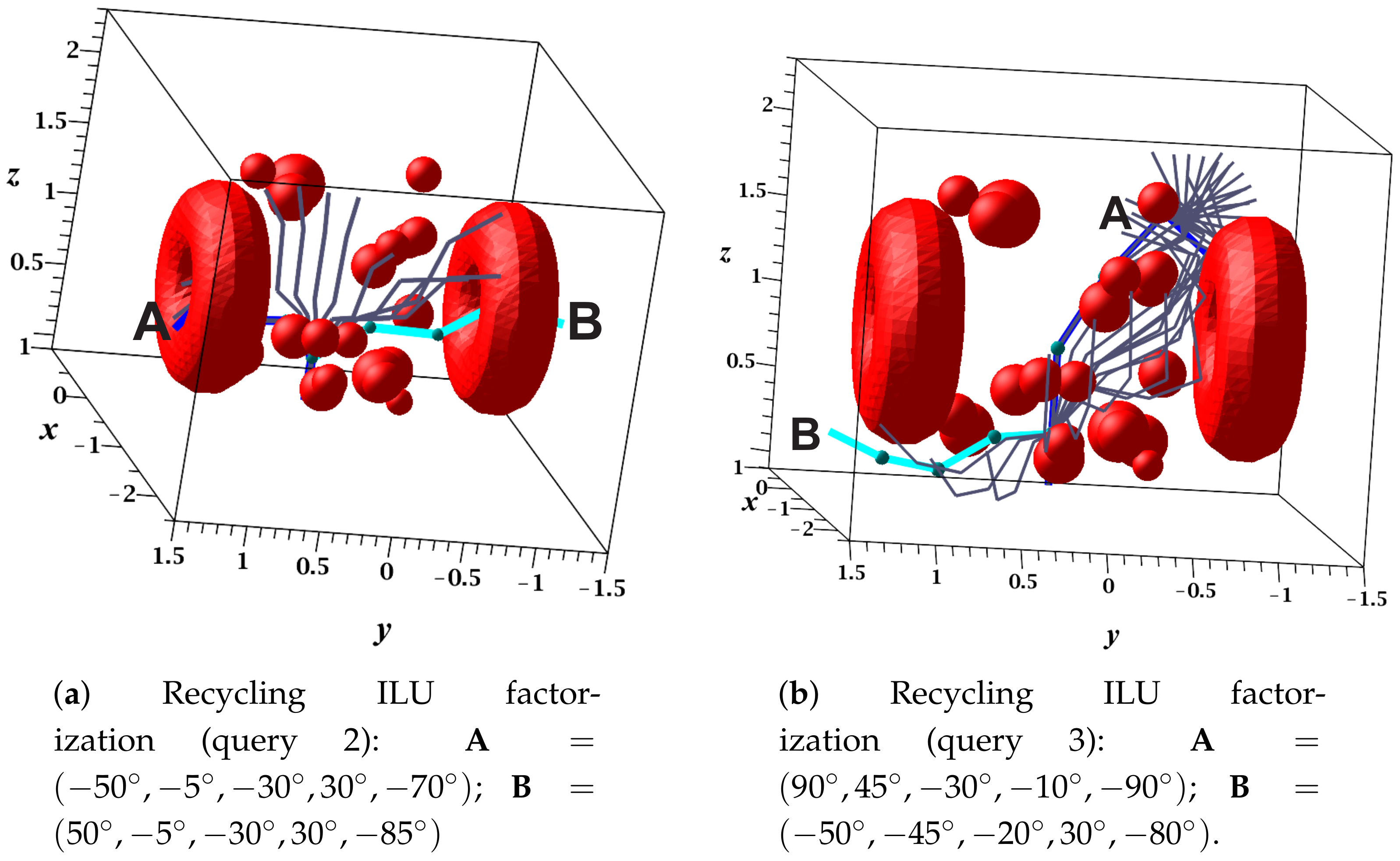
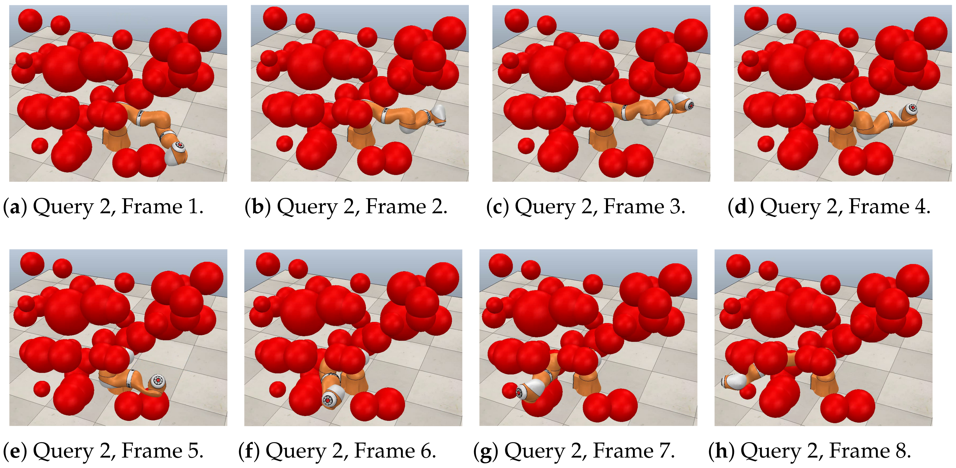
Figure 22.
Collision-free path for a KUKA manipulator. Query 2, and .
Figure 22.
Collision-free path for a KUKA manipulator. Query 2, and .
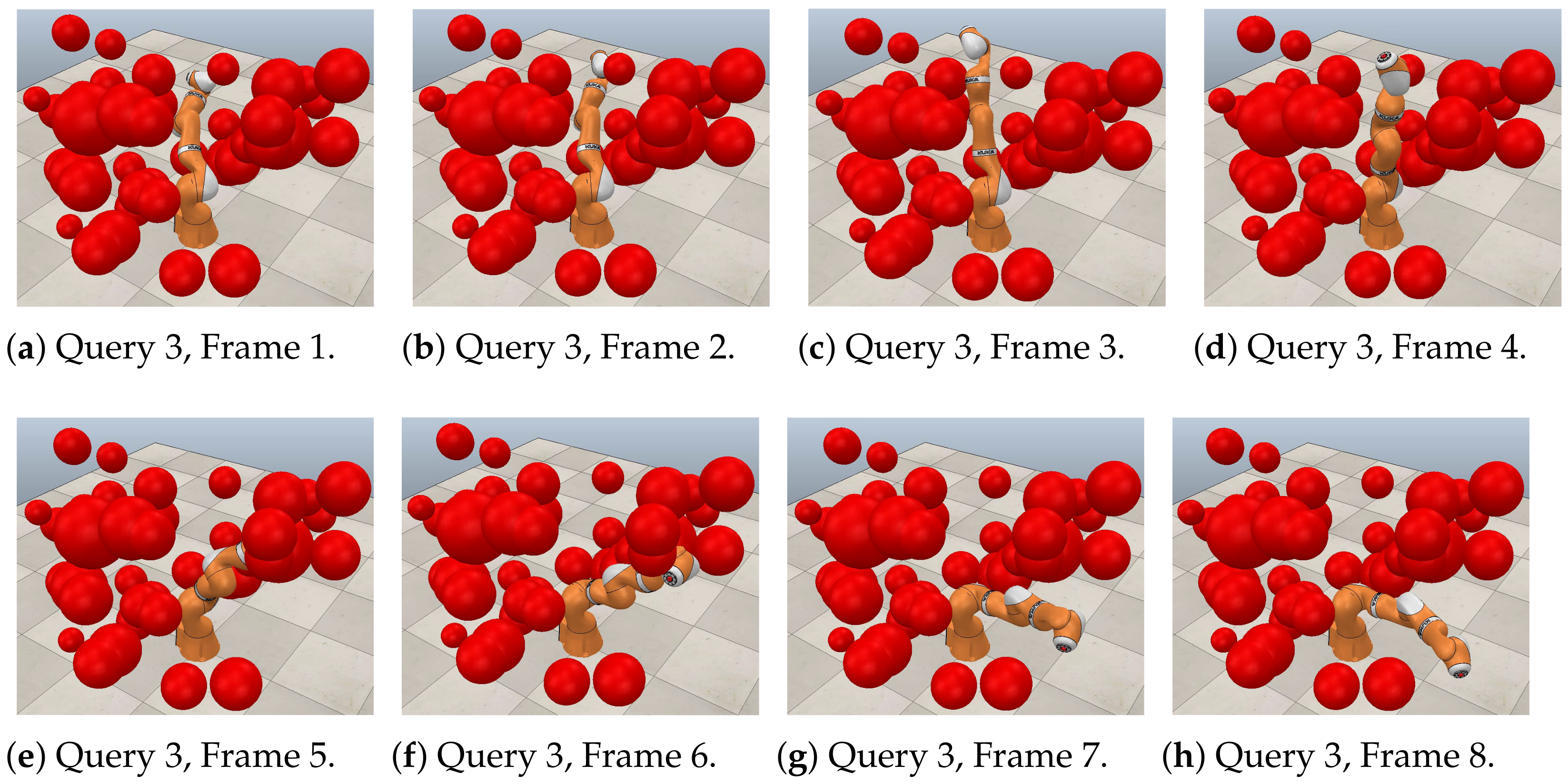
Figure 23.
Collision-free path for a KUKA manipulator. Query 3, and .
Figure 23.
Collision-free path for a KUKA manipulator. Query 3, and .
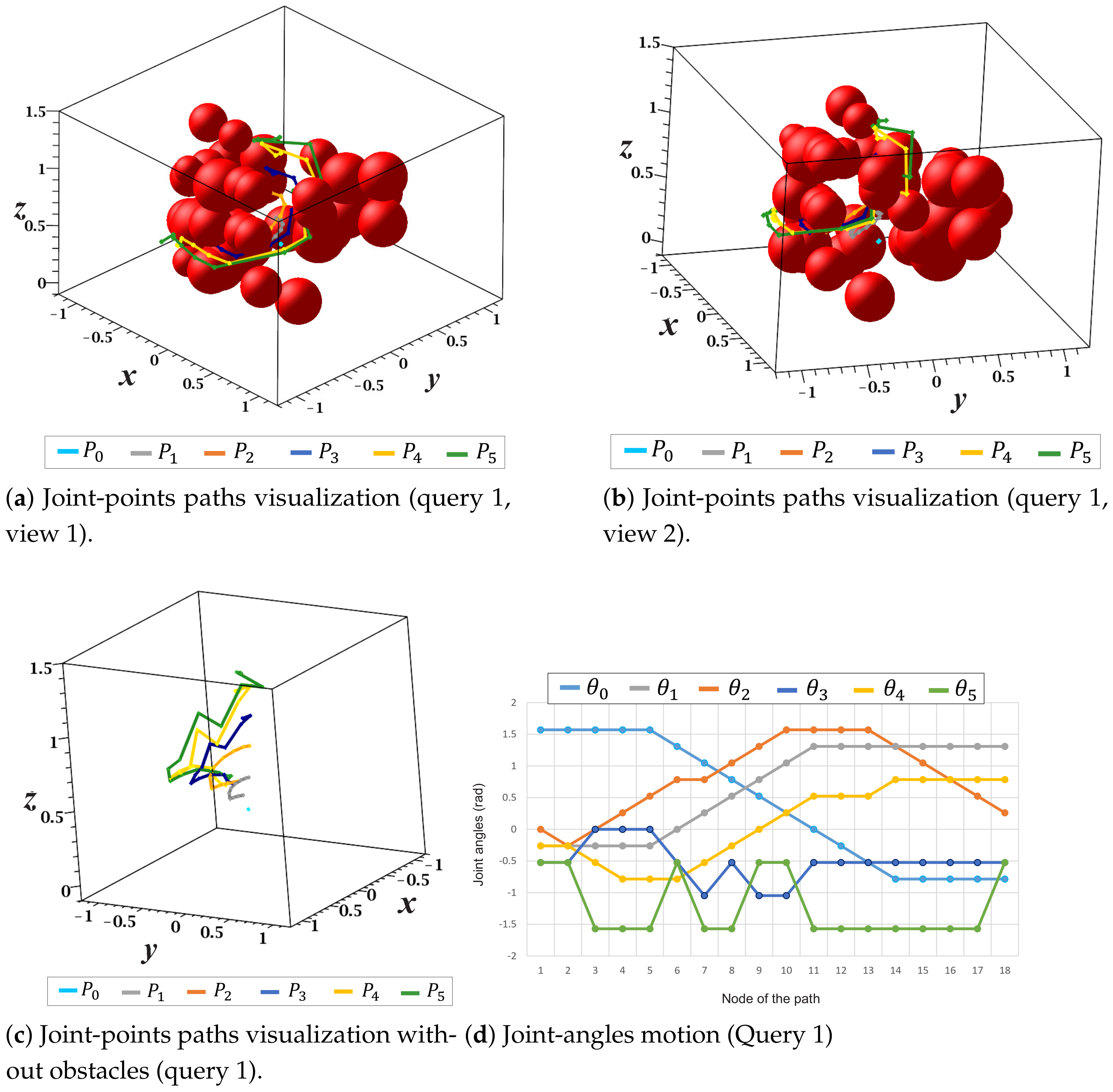
Figure 24.
Joint-points paths and joint-angles motion (query 1).
Figure 24.
Joint-points paths and joint-angles motion (query 1).
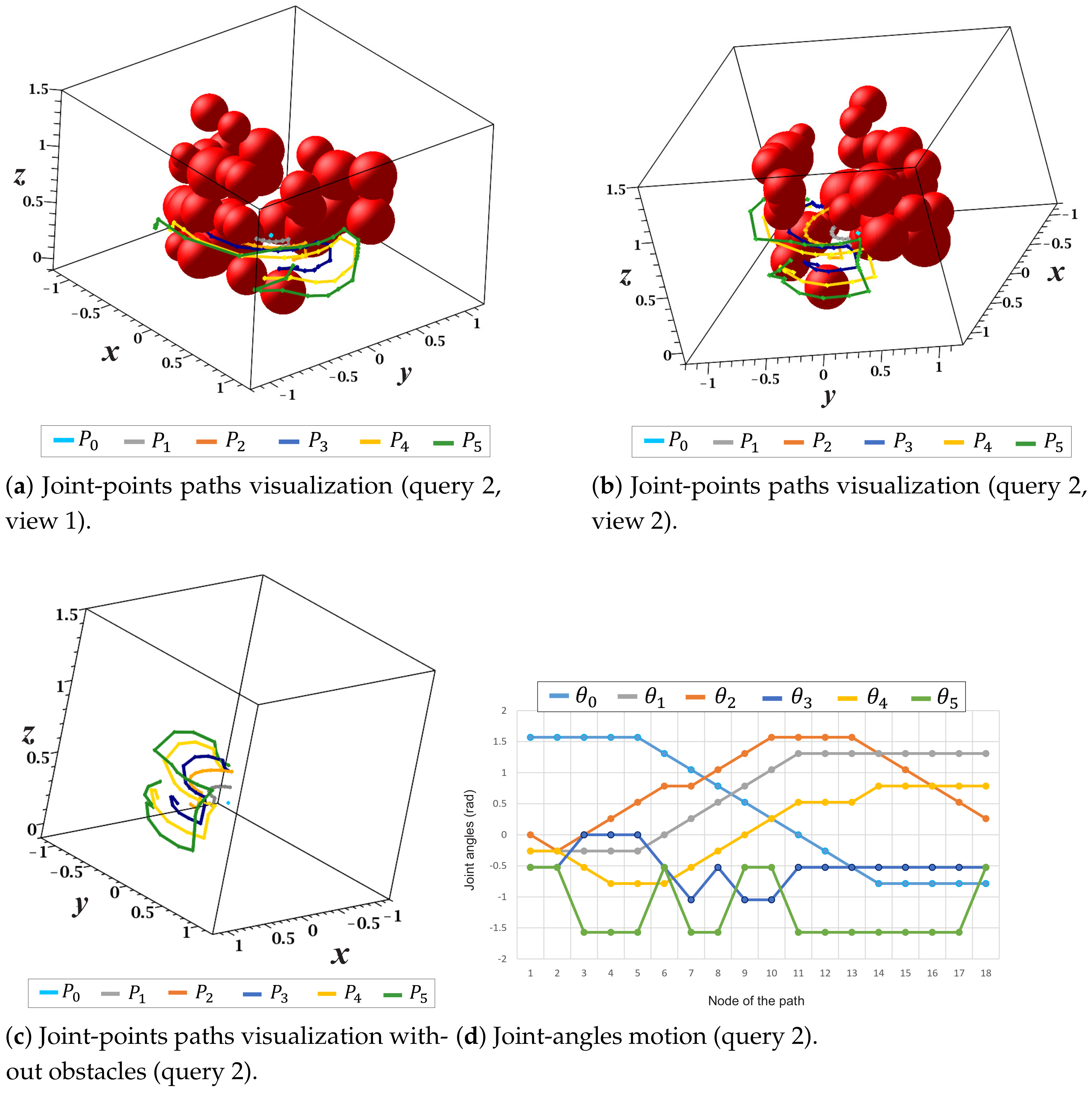
Figure 25.
Joint-points paths and joint-angles motion (query 2).
Figure 25.
Joint-points paths and joint-angles motion (query 2).
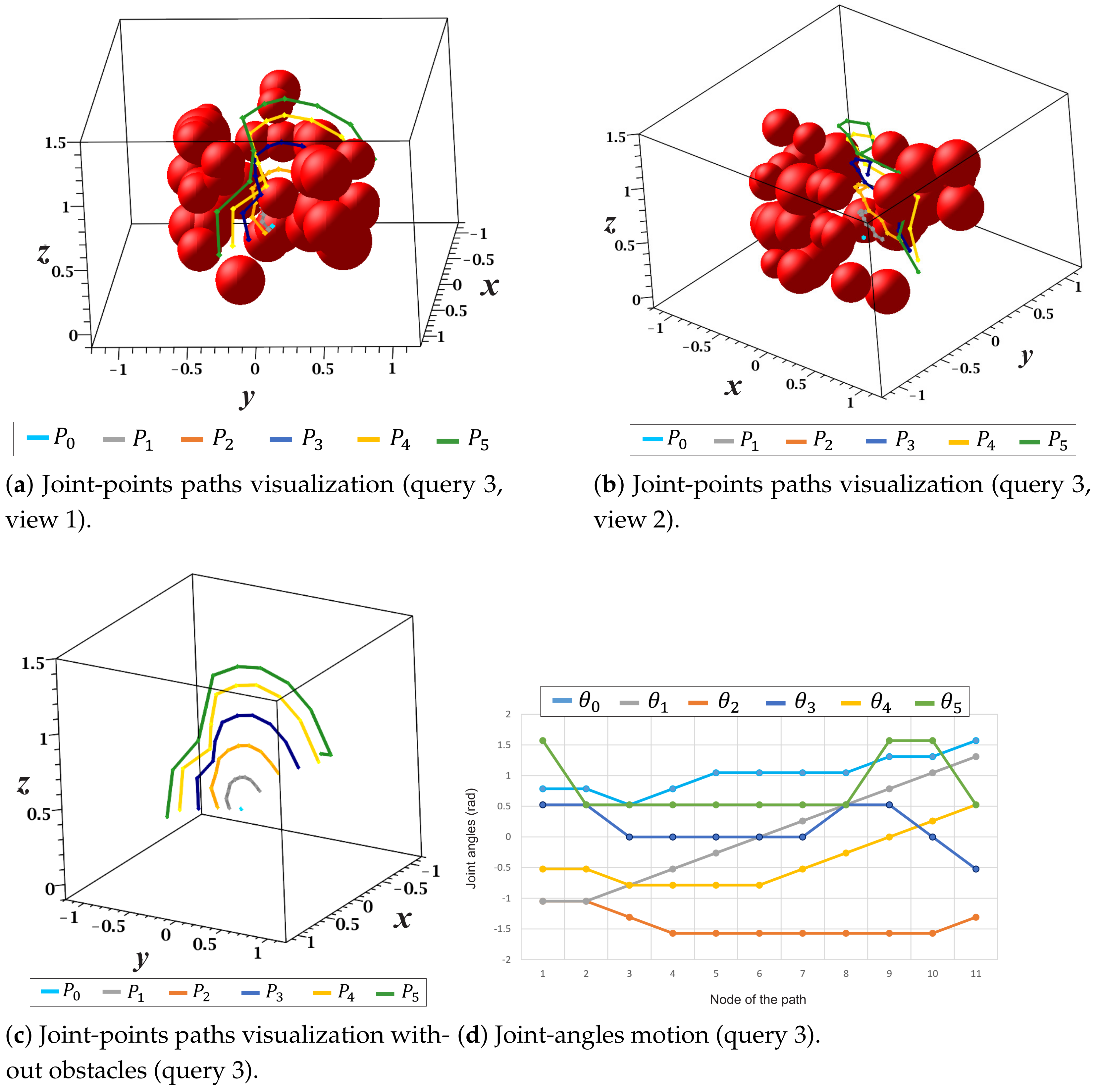
Figure 26.
Joint-points paths and joint-angles motion (query 3).
Figure 26.
Joint-points paths and joint-angles motion (query 3).
Table 1.
D-H parameters of a two-DOF manipulator.
Table 1.
D-H parameters of a two-DOF manipulator.
| Link i | Joint Angle | Twist Angle | Length of Linkages (m) | Offset of Linkages (m) | Angle Range |
|---|
| 1 | | | 0 | | |
| 2 | | | | 0 | |
Table 2.
D-H parameters of a 3 DOF manipulator.
Table 2.
D-H parameters of a 3 DOF manipulator.
| Link i | Joint Angle
| Twist Angle
| Length of
Linkages (m) | Offset of
Linkages (m) | Angle Range |
|---|
| 1 | | | 0 | | |
| 2 | | | | 0 | |
| 3 | | | | 0 | |
Table 3.
Execution time of case study 1 (3 DOF manipulator). ETBC: execution time of bitmap creation, ETPIB: execution time per iteration in the bitmap creation process, ET-MNA: execution time of MNA creation, ETPI-MNA: execution time per iteration in the MNA creation process.
Table 3.
Execution time of case study 1 (3 DOF manipulator). ETBC: execution time of bitmap creation, ETPIB: execution time per iteration in the bitmap creation process, ET-MNA: execution time of MNA creation, ETPI-MNA: execution time per iteration in the MNA creation process.
| No. Query | ETBC (s) | ETPIB (s) | ET-MNA (s) | ETPI-MNA (s) | No. Nodes | No. Resistors |
|---|
| 1 | | 0–0.0009982 | | 0–0.0019949 | 7291 | 59,953 |
Table 4.
Execution time of case study 1 (3 DOF manipulator). ETF: execution time spent in the incomplete LU factorization, ETS: execution time spent to solve linear system using ILU factors, ETLCC: execution time spent in the LCC algorithm, : ILU tolerance = , : ILU tolerance = .
Table 4.
Execution time of case study 1 (3 DOF manipulator). ETF: execution time spent in the incomplete LU factorization, ETS: execution time spent to solve linear system using ILU factors, ETLCC: execution time spent in the LCC algorithm, : ILU tolerance = , : ILU tolerance = .
| N. Query | ETF (s)|ETS (s) @α | ETF (s)|ETS (s) @β | ETLCC (s) (α|β) | Success (α|β) | Length (α|β) |
|---|
| 1 | 0.0459111|0.0019632 | 0.0478875|0.0009972 | 0.1665551|0.1625701 | Yes|Yes | 52|53 |
| 2 | − −|0.0009979 | − −|0.0010022 | − −|0.1695493 | No|Yes | − −|55 |
| 3 | − −|0.0009975 | − −|0.0019773 | 0.1047202|0.1017282 | Yes|Yes | 31|32 |
Table 5.
D-H parameters of the 5 DOF manipulator.
Table 5.
D-H parameters of the 5 DOF manipulator.
| Link i | Joint Angle
| Twist Angle
| Length of
Linkages (m) | Offset of
Linkages (m) | Angle Range |
|---|
| 1 | | | 0 | | |
| 2 | | | | 0 | |
| 3 | | | | 0 | |
| 4 | | | | 0 | |
| 5 | | | | 0 | |
Table 6.
Execution time of case study 2 (5 DOF manipulator). ETBC: execution time of bitmap creation, ETPIB: execution time per iteration in the bitmap creation process, ET-MNA: execution time of MNA creation, ETPI-MNA: execution time per iteration in the MNA creation process.
Table 6.
Execution time of case study 2 (5 DOF manipulator). ETBC: execution time of bitmap creation, ETPIB: execution time per iteration in the bitmap creation process, ET-MNA: execution time of MNA creation, ETPI-MNA: execution time per iteration in the MNA creation process.
| No. Query | ETBC (s) | ETPIB (s) | ET-MNA (s) | ETPI-MNA (s) | No. Nodes | No. Resistors |
|---|
| 1 | 3053.4698287 | 0–0.0086051 | | 0–0.0059847 | 313,958 | 17,127,851 |
Table 7.
Executiontime for case study 2 (5 DOF manipulator). ETF: execution time spent for the incomplete LU factorization, ETS: execution time spent to solve the linear system using ILU factors, ETLCC: execution time spent in the LCC algorithm, : ILU tolerance = , : ILU tolerance = .
Table 7.
Executiontime for case study 2 (5 DOF manipulator). ETF: execution time spent for the incomplete LU factorization, ETS: execution time spent to solve the linear system using ILU factors, ETLCC: execution time spent in the LCC algorithm, : ILU tolerance = , : ILU tolerance = .
| No. Query | ETF (s)|ETS (s) @α | ETF (s)|ETS (s) @β | ETLCC (s) (α|β) | Success (α|β) | Length (α|β) |
|---|
| 1 | 1521.8933052|0.2214086 | 6044.8255501|0.4538076 | 14.2039926|14.2133202 | Yes|Yes | 16|14 |
| 2 | − −|0.1456099 | − −|0.4757362 | − −|16.297971 | No|Yes | − −|13 |
| 3 | − −|0.1845103 | − −|0.4737734 | 45.4964143|50.0593325 | Yes|Yes | 34|36 |
Table 8.
D-H parameters of the KUKA 6 DOF manipulator.
Table 8.
D-H parameters of the KUKA 6 DOF manipulator.
| Link i | Joint Angle
| ; T, A. | Length of
Linkages (m) | Offset of
Linkages (m) | Angle Range |
|---|
| 1 | | | 0 | | |
| 2 | | | | 0 | |
| 3 | | | | 0 | |
| 4 | | | | 0 | |
| 5 | | | | 0 | |
| 6 | | | | 0 | |
Table 9.
Execution time of case study 3 (KUKA six-DOF manipulator). ETBC: execution time of bitmap creation, ETPIB: execution time per iteration in the bitmap creation process, ET-MNA: execution time of MNA creation, ETPI-MNA: execution time per iteration in the MNA creation process.
Table 9.
Execution time of case study 3 (KUKA six-DOF manipulator). ETBC: execution time of bitmap creation, ETPIB: execution time per iteration in the bitmap creation process, ET-MNA: execution time of MNA creation, ETPI-MNA: execution time per iteration in the MNA creation process.
| No. Query | ETBC (s) | ETPIB (s) | ET-MNA (s) | ETPI-MNA (s) | No. Nodes | No. Resistors |
|---|
| 1 | 2724.4385299 | 0–0.0100044 | | 0–0.0059834 | 204,087 | 30,335,568 |
Table 10.
Execution time of case study 3 (KUKA 6 DOF manipulator). ETF: execution time spent for the incomplete LU factorization, ETS: execution time spent to solve linear system using ILU factors, ETLCC: execution time spent in the LCC algorithm, : ILU tolerance = , and : ILU tolerance = .
Table 10.
Execution time of case study 3 (KUKA 6 DOF manipulator). ETF: execution time spent for the incomplete LU factorization, ETS: execution time spent to solve linear system using ILU factors, ETLCC: execution time spent in the LCC algorithm, : ILU tolerance = , and : ILU tolerance = .
| N. Query | ETF (s)|ETS (s) @α | ETF (s)|ETS (s) @β | ETLCC (s) (α|β) | Success (α|β) | Length (α|β) |
|---|
| 1 | 7185.3962328|0.8457383 | 8421.5324378|0.9041367 | − −|24.8436352 | No|Yes | − −|18 |
| 2 | − −|0.8387568 | − −|0.8330152 | 35.4426557|43.276417 | Yes|Yes | 28|28 |
| 3 | − −|2.1003303 | − −|0.8520035 | 17.8586804|23.271181 | Yes|Yes | 11|12 |


 ,
, 


