Theoretical Identification of Coupling Effect and Performance Analysis of Single-Source Direct Sampling Method

Abstract

Although the direct sampling method (DSM) has demonstrated its feasibility in identifying small anomalies from measured scattering parameter data in microwave imaging, inaccurate imaging results that cannot be explained by conventional research approaches have often emerged. It has been heuristically identified that the reason for this phenomenon is due to the coupling effect between the antenna and dipole antennas, but related mathematical theory has not been investigated satisfactorily yet. The main purpose of this contribution is to explain the theoretical elucidation of such a phenomenon and to design an improved DSM for successful application to microwave imaging. For this, we first survey traditional DSM and design an improved DSM, which is based on the fact that the measured scattering parameter is influenced by both the anomaly and the antennas. We then establish a new mathematical theory of both the traditional and the designed indicator functions of DSM by constructing a relationship between the antenna arrangement and an infinite series of Bessel functions of integer order of the first kind. On the basis of the theoretical results, we discover various factors that influence the imaging performance of traditional DSM and explain why the designed indicator function successfully improves the traditional one. Several numerical experiments with synthetic data support the established theoretical results and illustrate the pros and cons of traditional and designed DSMs.

1. Introduction

The main purpose of microwave imaging is to retrieve the parameter (permittivity or conductivity) distribution in a domain from scattering parameter data. This is an old and difficult problem due to its intrinsic ill-posedness and nonlinearity [1]. Nevertheless, it is a very important problem to current scientists and engineers in developing reliable tools and techniques that can be applied to real-world problems such as medical imaging [2,3,4], damage detection in civil structure [5,6,7], radar imaging [8,9,10], etc. In order to solve this problem, various techniques have proposed various reconstruction algorithms. For example, Newton method [11] for reconstructing crack shape, Gauss–Newton method for 3D imaging [12] and biomedical imaging [13], Levenberg–Marquadt algorithm for detection and monitoring of leukemia [14] and reconstructing permittivity distribution [15], level-set technique [16] for inverse scattering problem, and optimal control approach [17] for reconstructing extended targets.

For a successful application of iterative-based techniques, one must begin the iteration procedure with a good initial guess. Otherwise, they will encounter the nonconvergence issue or the occurrence of a local minimizer. Moreover, a huge amount of computational cost will be required to perform the large number of iteration procedures; refer to [18]. Hence, it is natural to consider the generation of a good initial guess before the iteration procedure. Due to this reason, various noniterative techniques have been investigated and applied to inverse scattering problems and microwave imaging, for example, MUltiple SIgnal Classification (MUSIC) algorithm [19,20], Kirchhoff and subspace migrations [21,22], Factorization method [23,24], topological sensitivity [25,26], and linear sampling method [27,28].

Direct sampling method (DSM) is a fast, effective, and stable noniterative technique for identifying the location or the outline shape of small or extended targets related to various inverse problems. As such, DSM is currently widely applied in many fields, including the identification of two- and three-dimensional small scatterers [29,30,31,32,33,34] or perfectly conducting cracks [35], diffusive optical tomography [36], electrical impedance tomography [37], detecting sources in a stratified ocean waveguide [38], phaseless inverse source scattering problem [39], and mono-static imaging [40].

Recently, the application of DSM has been extended to microwave imaging that uses synthetic [41] and real [42] data for a noniterative identification of small anomalies from the collected scattering parameter data. The rapid identification of unknown anomalies is crucial in microwave imaging and DSM can be regarded as a suitably fast microwave imaging technique because it has certain advantages, such as the requirement of only a few (e.g., one or two) sources for generating incident fields and the low computational cost for performing the imaging procedure. However, difficulties can emerge in terms of identifying why inaccurate results had been obtained (see [41,43]). Heuristically, it has turned out that this phenomenon is due to the coupling effect between the anomaly and antennas, and the distance between the transmitter and the anomaly. However, a related mathematical theory of this phenomenon has yet to be satisfactorily established because previous studies do not consider the coupling effect between teh anomaly and antennas. Motivated by this issue, we attempted to identify the factors that influence the measurement data and correspondingly introduced another indicator function of DSM for a better imaging performance by removing certain scattering parameter data influenced by the coupling effect. This is based on the hypothesis that there exists a coupling effect between anomaly and antennas. We subsequently determined the mathematical structure of both the traditional and the introduced indicator functions by establishing relationships among the Bessel functions of the integer order of the first kind, the antenna setting, and the material properties. The theoretical results revealed the reason behind the appearance of inaccurate results using the traditional DSM and allowed for achieving a better imaging performance with the introduced indicator function.

Various simulation results from synthetic data generated by the CST STUDIO SUITE demonstrate the theoretical result and explored behaviors of traditional and designed DSM. It is worth emphasizing that once the outline shape of the anomaly is recognized, it can be selected as a good initial guess and one can retrieve a complete shape via iteration-based schemes.

The remainder of this paper is organized as follows. In Section 2, we outline the basic concept of the scattering parameter, introduce the traditional indicator functions of DSM, and design another DSM indicator function for improving the imaging performance. In Section 3, we investigate the structure of the indicator functions by establishing relationships among the Bessel functions of the integer order of the first kind, the antenna configuration, and the material properties. In Section 4, a set of simulation results with synthetic data are presented to support the investigation. A short conclusion including an outline of the current and future work is given in Section 5.

2. Scattering Parameter and Indicator Functions of Direct Sampling Method

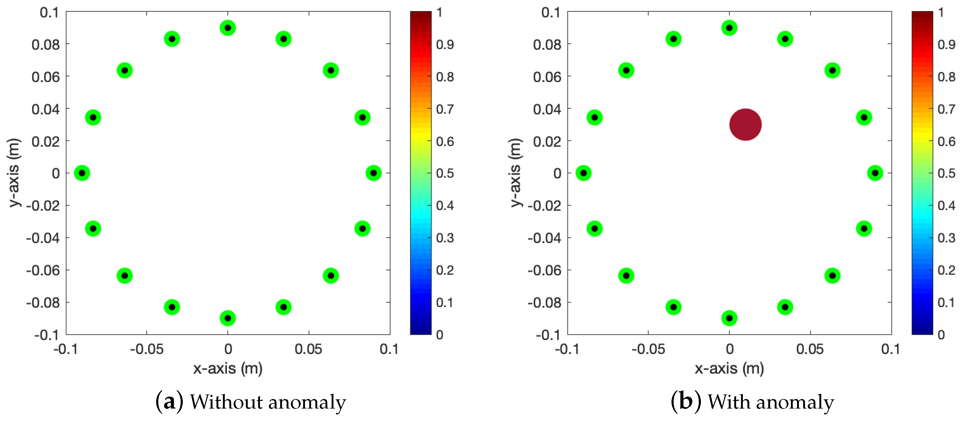
Suppose that there exists a circular cylindrical obstacle with infinite length in the vertical direction (parallel to the z-axis) in a given region of interest (ROI) and it is surrounded by a number of dipole antennas in the vertical direction. Then, based on mathematical treatment of the scattering of time-harmonic electromagnetic waves from thin infinitely long cylindrical obstacles, this can be considered the two-dimensional inverse problem. An illustration of the experimental setup and the two-dimensional cross-section of the obstacle is given in Figure 1; refer to [20] for a detailed description.

We denote $\mathcal{D}$ as the 2D cross section of a cylindrical obstacle with radius $\alpha$ and location ${\mathbf{r}}_{★}\in \Omega$ such that

$$\mathcal{D}={\mathbf{r}}_{★}+\alpha \mathbf{B},$$

where $\mathbf{B}$ denotes the two-dimensional unit circle centered at the origin (in general, $\mathbf{B}$ is a simply connected domain with smooth boundary that describes the shape of $\mathcal{D}$) and ${\mathcal{A}}_n\in \mathrm{Ext}(\Omega )$ is the dipole antenna located at ${\mathbf{a}}_n$, $n=1,2,\cdots ,N$ to transmit or receive signals. Here, $\Omega$ denotes the homogeneous background, which is the intersection between the ROI and ${\mathbb{R}}^2$, and $\mathrm{Ext}(\Omega )$ is the exterior of $\Omega$. Throughout this paper, we consider the single-source case, i.e., an antenna ${\mathcal{A}}_m$ is used for signal transmission only and the antennas ${\mathcal{A}}_n$, $n=1,2,\cdots ,N$ are used for signal reception.

All materials involved are nonmagnetic i.e., they are characterized by their dielectric permittivity and electrical conductivity at a given angular frequency $\omega =2\pi f$. Correspondingly, we set the value of magnetic permeability to be constant at every location $\mathbf{r}\in \Omega$ such that $\mu \left(\mathbf{r}\right)={\mu }_{\mathrm{b}}=1.256\times {10}^{-6} \mathrm{H}/\mathrm{m}$. Meanwhile, we denote ${\epsilon }_{★}={\epsilon }_{\mathbf{r}★}·{\epsilon }_0$ and ${\epsilon }_{\mathrm{b}}={\epsilon }_{rb}·{\epsilon }_0$ as the permittivity of $\mathcal{D}$ and the $\Omega$, respectively, where ${\epsilon }_0=8.854\times {10}^{-12} \mathrm{F}/\mathrm{m}$ is the vacuum permittivity. The conductivities ${\sigma }_{★}$ and ${\sigma }_{\mathrm{b}}$ could then be defined analogously. Following this, we introduce the piecewise constant permittivity $\epsilon \left(\mathbf{r}\right)$ and conductivity $\sigma \left(\mathbf{r}\right)$ as follows:

$$\epsilon \left(\mathbf{r}\right)=\left\{\begin{array}{ccc}\hfill {\epsilon }_{★}& if& \mathbf{r}\in \mathcal{D}\hfill \\ \hfill {\epsilon }_{\mathrm{b}}& if& \mathbf{r}\in \Omega \backslash \mathcal{D}\hfill \end{array}\right.and\sigma \left(\mathbf{r}\right)=\left\{\begin{array}{ccc}\hfill {\sigma }_{★}& if& \mathbf{r}\in \mathcal{D}\hfill \\ \hfill {\sigma }_{\mathrm{b}}& if& \mathbf{r}\in \Omega \backslash \mathcal{D},\hfill \end{array}\right.$$

respectively. With this, let k be the background wave number that satisfies $k^2={\omega }^2{\mu }_{\mathrm{b}}({\epsilon }_{\mathrm{b}}+i{\sigma }_{\mathrm{b}}/\omega )$ and assume that $\omega {\epsilon }_{\mathrm{b}}\gg {\sigma }_{\mathrm{b}}$.

Let us denote ${\mathrm{S}}_{scat}(n,m)$ as the S-parameter (or scattering parameter) defined as

$${\mathrm{S}}_{scat}(n,m)=\frac{{\mathrm{V}}_n^{-}}{{\mathrm{V}}_m^{+}},$$

where ${\mathrm{V}}_m^{+}$ denotes the input voltage (or incident wave) at ${\mathcal{A}}_m$ and ${\mathrm{V}}_n^{-}$ is the corresponding output voltage (or reflected wave) at ${\mathcal{A}}_n$. We also denote ${\mathrm{S}}_{tot}(n,m)$ and ${\mathrm{S}}_{inc}(n,m)$ as the total and incident S-parameters in the presence and absence of $\mathcal{D}$. Throughout this paper, the measurement data are the scattered-field S-parameter defined as

$${\mathrm{S}}_{scat}(n,m)={\mathrm{S}}_{tot}(n,m)-{\mathrm{S}}_{inc}(n,m).$$

Note that this subtraction is essential to remove unknown modeling errors and is useful in designing an indicator function because it can be expressed as the following integral equation:

$${\mathrm{S}}_{scat}(n,m)=\frac{i{k}^2}{4\omega {\mu }_{\mathrm{b}}}{\int }_{\Omega }\mathcal{O}\left(\mathbf{r}\right){\mathrm{E}}_{inc}^{\left(z\right)}({\mathbf{a}}_m,\mathbf{r}){\mathrm{E}}_{tot}^{\left(z\right)}(\mathbf{r},{\mathbf{a}}_n)d\mathbf{r},$$

(1)

where $\mathcal{O}\left(\mathbf{r}\right)$ denotes the objective function

$$\mathcal{O}\left(\mathbf{r}\right)=\frac{\epsilon \left(\mathbf{r}\right)-{\epsilon }_b}{{\epsilon }_{\mathrm{b}}}+i\frac{\sigma \left(\mathbf{r}\right)-{\sigma }_{\mathrm{b}}}{\omega {\epsilon }_{\mathrm{b}}},$$

${\mathrm{E}}_{inc}^{\left(z\right)}({\mathbf{a}}_m,\mathbf{r})$ denote the z-component of the incident field ${\mathbf{E}}_{inc}({\mathbf{a}}_m,\mathbf{r})$ in a homogeneous medium due to the point current density at ${\mathcal{A}}_m$, and ${\mathrm{E}}_{tot}^{\left(z\right)}(\mathbf{r},{\mathbf{a}}_n)$ is the z-component of the total field ${\mathbf{E}}_{tot}(\mathbf{r},{\mathbf{a}}_n)$. Notice that, based on the Maxwell equation, the incident field ${\mathbf{E}}_{inc}({\mathbf{a}}_m,\mathbf{r})\in {\mathbb{C}}^{1\times 3}$ satisfies

$$curl{\mathbf{E}}_{inc}({\mathbf{a}}_m,\mathbf{r})=-i\omega {\mu }_{\mathrm{b}}{\mathbf{H}}_{inc}({\mathbf{a}}_m,\mathbf{r})\mathrm{and}curl{\mathbf{H}}_{inc}({\mathbf{a}}_m,\mathbf{r})=({\sigma }_{\mathrm{b}}+i\omega {\epsilon }_{\mathrm{b}}){\mathbf{E}}_{inc}({\mathbf{a}}_m,\mathbf{r})$$

and the corresponding total field ${\mathbf{E}}_{tot}(\mathbf{r},{\mathbf{a}}_n)\in {\mathbb{C}}^{1\times 3}$ satisfies

$$curl{\mathbf{E}}_{tot}(\mathbf{r},{\mathbf{a}}_n)=-i\omega {\mu }_{\mathrm{b}}{\mathbf{H}}_{tot}(\mathbf{r},{\mathbf{a}}_n)\mathrm{and}curl{\mathbf{H}}_{tot}(\mathbf{r},{\mathbf{a}}_n)=(\sigma \left(\mathbf{r}\right)+i\omega \epsilon \left(\mathbf{r}\right)){\mathbf{E}}_{tot}(\mathbf{r},{\mathbf{a}}_n),$$

with a transmission condition at the boundary $\partial \mathcal{D}$. Here, ${\mathbf{H}}_{inc}$ and ${\mathbf{H}}_{tot}$ denote the magnetic fields defined analogously.

At this moment, we cannot use ${\mathrm{S}}_{scat}(n,m)$ to design an indicator function because the total field ${\mathrm{E}}_{tot}^{\left(z\right)}(\mathbf{r},{\mathbf{a}}_n)$ of (1) cannot be formulated without a priori information of $\mathcal{D}$. Now, let us assume that the cross section $\mathcal{D}$ is a small ball such that

$$\left(\sqrt{\frac{{\epsilon }_{★}}{{\epsilon }_{\mathrm{b}}}-1}\right)\alpha <\frac{\lambda }{4},$$

where $\lambda$ denotes the background wavelength. Then, based on [44], it is possible to apply the Born approximation so that the total field ${\mathrm{E}}_{tot}^{\left(z\right)}(\mathbf{r},{\mathbf{a}}_n)$ can be approximated by the incident field ${\mathrm{E}}_{inc}^{\left(z\right)}(\mathbf{r},{\mathbf{a}}_n)$. With this, on the basis of the reciprocity property of the incident field, ${\mathrm{S}}_{scat}(n,m)$ can be approximated as follows:

$$\begin{array}{cc}\hfill {\mathrm{S}}_{scat}(n,m)& \approx \frac{i{k}^2}{4\omega {\mu }_{\mathrm{b}}}{\int }_{\Omega }\mathcal{O}\left(\mathbf{r}\right){\mathrm{E}}_{inc}^{\left(z\right)}({\mathbf{a}}_m,\mathbf{r}){\mathrm{E}}_{inc}^{\left(z\right)}(\mathbf{r},{\mathbf{a}}_n)d\mathbf{r}\hfill \\ \hfill & \approx \frac{i{k}^2}{4\omega {\mu }_{\mathrm{b}}}area\left(\mathcal{D}\right)\mathcal{O}\left({\mathbf{r}}_{★}\right){\mathrm{E}}_{inc}^{\left(z\right)}({\mathbf{a}}_m,{\mathbf{r}}_{★}){\mathrm{E}}_{inc}^{\left(z\right)}({\mathbf{r}}_{★},{\mathbf{a}}_n)\hfill \\ \hfill & =\frac{i{k}^2}{4\omega {\mu }_{\mathrm{b}}}area\left(\mathcal{D}\right)\mathcal{O}\left({\mathbf{r}}_{★}\right){\mathrm{E}}_{inc}^{\left(z\right)}({\mathbf{a}}_m,{\mathbf{r}}_{★}){\mathrm{E}}_{inc}^{\left(z\right)}({\mathbf{a}}_n,{\mathbf{r}}_{★}).\hfill \end{array}$$

(2)

Let $\mathsf{\Gamma }$ be the set of measurement data $\mathsf{\Gamma }=\left\{{\mathrm{S}}_{scat}(n,m):n=1,2,\cdots ,N\right\}$ and $\mathbf{U}$ be the unit vector, which is the arrangement of measurement datain $\mathsf{\Gamma }$:

$$\mathbf{U}=\frac{1}{\left|\right|{\mathrm{S}}_{scat}(n,m){\left|\right|}_{{\ell }^2\left(\mathsf{\Gamma }\right)}}{\left[{\mathrm{S}}_{scat}(1,m),{\mathrm{S}}_{scat}(2,m),\cdots ,{\mathrm{S}}_{scat}(N,m)\right]}^T,$$

where the inner product and corresponding norm are defined as

$${\langle f\left(n\right),g\left(n\right)\rangle }_{{\ell }^2\left(\mathsf{\Gamma }\right)}=\sum _{n=1}^{N}f\left(n\right)\overline{g\left(n\right)}{\mathrm{and}\left|\right|·\left|\right|}_{{\ell }^2\left(\mathsf{\Gamma }\right)}=\sqrt{{\langle ·,·\rangle }_{{\ell }^2\left(\mathsf{\Gamma }\right)}},$$

(3)

respectively. Then, based on (2), $\mathbf{U}$ can be written by

$$\mathbf{U}=\frac{i{k}^{2}area\left(\mathcal{D}\right)\mathcal{O}\left({\mathbf{r}}_{★}\right)}{4\omega {\mu }_{\mathrm{b}}\left|\right|{\mathrm{S}}_{scat}(n,m){\left|\right|}_{{\ell }^2\left(\mathsf{\Gamma }\right)}}{\mathrm{E}}_{inc}^{\left(z\right)}({\mathbf{a}}_m,{\mathbf{r}}_{★}){\left[{\mathrm{E}}_{inc}^{\left(z\right)}({\mathbf{a}}_1,{\mathbf{r}}_{★}),{\mathrm{E}}_{inc}^{\left(z\right)}({\mathbf{a}}_2,{\mathbf{r}}_{★}),\cdots ,{\mathrm{E}}_{inc}^{\left(z\right)}({\mathbf{a}}_N,{\mathbf{r}}_{★})\right]}^T.$$

Based on the above expression, let us define the following unit vector: for $\mathbf{r}\in \Omega$

$$\mathbf{W}\left(\mathbf{r}\right)=\frac{1}{\left|\right|{\mathrm{E}}_{inc}^{\left(z\right)}({\mathbf{a}}_n,\mathbf{r}){\left|\right|}_{{\ell }^2\left(\mathsf{\Gamma }\right)}}{\left[{\mathrm{E}}_{inc}^{\left(z\right)}({\mathbf{a}}_1,\mathbf{r}),{\mathrm{E}}_{inc}^{\left(z\right)}({\mathbf{a}}_2,\mathbf{r}),\cdots ,{\mathrm{E}}_{inc}^{\left(z\right)}({\mathbf{a}}_N,\mathbf{r})\right]}^T.$$

Then, by testing orthonormality relation between $\mathbf{U}$ and $\mathbf{W}\left(\mathbf{r}\right)$, it will be possible to extract ${\mathbf{r}}_{★}$ so that the location of $\mathcal{D}$ can be identified. To this end, the typical indicator function ${\mathfrak{F}}_{DSM}(\mathbf{r},m)$ has been designed as follows (see [29,30,31,33]):

$${\mathfrak{F}}_{DSM}(\mathbf{r},m)=\left|\mathbf{U}·\overline{\mathbf{W}}\left(\mathbf{r}\right)\right|=\frac{|{\langle {\mathrm{S}}_{scat}(n,m),{\mathrm{E}}_{inc}^{\left(z\right)}({\mathbf{a}}_n,\mathbf{r})\rangle }_{{\ell }^2\left(\mathsf{\Gamma }\right)}|}{\left|\right|{\mathrm{S}}_{scat}{(n,m)\left|\right|}_{{\ell }^2\left(\mathsf{\Gamma }\right)}\left|\right|{\mathrm{E}}_{inc}^{\left(z\right)}({\mathbf{a}}_n,\mathbf{r}){\left|\right|}_{{\ell }^2\left(\mathsf{\Gamma }\right)}}.$$

Then, it is expected that the map ${\mathfrak{F}}_{DSM}(\mathbf{r},m)$ will contain a peak of largest magnitude 1 at $\mathbf{r}={\mathbf{r}}_{★}\in \mathcal{D}$ and a small magnitude at $\mathbf{r}\in \Omega \backslash \mathcal{D}$ so that the location $\mathcal{D}$ can be identified via the map of ${\mathfrak{F}}_{DSM}(\mathbf{r},m)$.

However, judging by the simulation results presented in Section 4, the imaging performance of ${\mathfrak{F}}_{DSM}(\mathbf{r},m)$ is somehow poor. Note that the imaging performance of ${\mathfrak{F}}_{DSM}(\mathbf{r},m)$ significantly depends on the location of the source ${\mathcal{A}}_m$. Moreover, if the antenna ${\mathcal{A}}_m$ is used for both signal transmission and reception, the measurement data ${\mathrm{S}}_{scat}(m,m)$ will be influenced not only by the anomaly but also by the other antennas ${\mathcal{A}}_n$, $n\ne m$. In contrast, if $m\ne n$, ${\mathrm{S}}_{scat}(n,m)$ is influenced by the anomaly only. For a detailed description, refer to ([21] Section 1). Hence, it is feasible to design a new indicator function by disregarding the measurement data ${\mathrm{S}}_{scat}(m,m)$, i.e., an antenna ${\mathcal{A}}_m$ is used for signal transmission only and the antennas ${\mathcal{A}}_n$, $n=1,2,\cdots ,N$ and $n\ne m$, are used for signal reception. With this, let us introduce the set of measurement data ${\mathsf{\Gamma }}_m=\left\{{\mathrm{S}}_{scat}(n,m):n=1,2,\cdots ,N,n\ne m\right\}$ and an arrangement of measurement data:

$$\begin{array}{c}{\mathbf{U}}_m=\frac{1}{\left|\right|{\mathrm{S}}_{scat}(n,m){\left|\right|}_{{\ell }^2\left({\mathsf{\Gamma }}_m\right)}}[{\mathrm{S}}_{scat}(1,m),{\mathrm{S}}_{scat}(2,m),\cdots ,\hfill \\ \hfill {\mathrm{S}}_{scat}(m-1,m),{\mathrm{S}}_{scat}(m+1,m),\cdots {\mathrm{S}}_{scat}(N,m){]}^T,\end{array}$$

where the inner product and corresponding norm are defined as

$$\begin{array}{c}\hfill \begin{array}{c}\hfill {\langle f\left(n\right),g\left(n\right)\rangle }_{{\ell }^2\left({\mathsf{\Gamma }}_m\right)}=\sum _{n=1,n\ne m}^{N}f\left(n\right)\overline{g\left(n\right)}{\mathrm{and}\left|\right|f\left(n\right)\left|\right|}_{{\ell }^2\left({\mathsf{\Gamma }}_m\right)}=\sqrt{{\langle f\left(n\right),f\left(n\right)\rangle }_{{\ell }^2\left({\mathsf{\Gamma }}_m\right)}},\end{array}\end{array}$$

(4)

respectively. Based on the structure of ${\mathbf{U}}_m$, let us introduce the following unit vector: for $\mathbf{r}\in \Omega$

$$\begin{array}{c}{\mathbf{W}}_m\left(\mathbf{r}\right)=\frac{1}{\left|\right|{\mathrm{E}}_{inc}^{\left(z\right)}({\mathbf{a}}_n,\mathbf{r}){\left|\right|}_{{\ell }^2\left({\mathsf{\Gamma }}_m\right)}}[{\mathrm{E}}_{inc}^{\left(z\right)}({\mathbf{a}}_1,\mathbf{r}),{\mathrm{E}}_{inc}^{\left(z\right)}({\mathbf{a}}_2,\mathbf{r}),\cdots ,\hfill \\ \hfill {\mathrm{E}}_{inc}^{\left(z\right)}({\mathbf{a}}_{m-1},\mathbf{r}),{\mathrm{E}}_{inc}^{\left(z\right)}({\mathbf{a}}_{m+1},\mathbf{r}),\cdots ,{\mathrm{E}}_{inc}^{\left(z\right)}({\mathbf{a}}_N,\mathbf{r}){]}^T\end{array}$$

and corresponding indicator function ${\mathfrak{F}}_{DSE}(\mathbf{r},m)$ such that

$${\mathfrak{F}}_{DSE}(\mathbf{r},m)=\left|{\mathbf{U}}_m·{\overline{\mathbf{W}}}_m\left(\mathbf{r}\right)\right|=\frac{|{\langle {\mathrm{S}}_{scat}(n,m),{\mathrm{E}}_{inc}^{\left(z\right)}({\mathbf{a}}_m,\mathbf{r})\rangle }_{{\ell }^2\left({\mathsf{\Gamma }}_m\right)}|}{\left|\right|{\mathrm{S}}_{scat}{(n,m)\left|\right|}_{{\ell }^2\left({\mathsf{\Gamma }}_m\right)}\left|\right|{\mathrm{E}}_{inc}^{\left(z\right)}({\mathbf{a}}_m,\mathbf{r}){\left|\right|}_{{\ell }^2\left({\mathsf{\Gamma }}_m\right)}}.$$

Then, it is expected that the imaging performance of ${\mathfrak{F}}_{DSE}(\mathbf{r},m)$ is better than the traditional performance of ${\mathfrak{F}}_{DSM}(\mathbf{r},m)$.

3. Theoretical Results and Related Discussion

To compare the imaging performance of ${\mathfrak{F}}_{DSM}(\mathbf{r},m)$ and ${\mathfrak{F}}_{DSE}(\mathbf{r},m)$, we established a mathematical structure of the indicator functions, as outlined below.

Theorem 1 (Structure of the indicator functions with single source).

Let $\mathbf{r}-{\mathbf{r}}_{★}=|\mathbf{r}-{\mathbf{r}}_{★}|{[cos{\varphi }_{★},sin{\varphi }_{★}]}^T$, $\mathbf{r}-{\mathbf{a}}_m=|\mathbf{r}-{\mathbf{a}}_m|{[cos{\varphi }_m,sin{\varphi }_m]}^T$, ${\theta }_n={\mathbf{a}}_n/\left|{\mathbf{a}}_n\right|={[cos{\theta }_n,sin{\theta }_n]}^T$, and $|{\mathbf{a}}_n|=R$ for all n. If ${\mathbf{a}}_n$ satisfies $\left|k\right({\mathbf{a}}_n-\mathbf{r}\left)\right|\gg 1/4$ for $n=1,2,\cdots ,N$ and $k=k_1+i{k}_2$, $k_1,k_2>0$, then the following relations hold uniformly:

$${\mathfrak{F}}_{DSM}(\mathbf{r},m)\approx \frac{|{\Phi }_1\left(\mathbf{r}\right)+{\Phi }_2\left(\mathbf{r}\right)|}{{\displaystyle \underset{\mathbf{r}\in \Omega }{max}|{\Phi }_1\left(\mathbf{r}\right)+{\Phi }_2\left(\mathbf{r}\right)|}}\mathrm{and}{\mathfrak{F}}_{DSE}(\mathbf{r},m)\approx \frac{|{\Phi }_3\left(\mathbf{r}\right)|}{{\displaystyle \underset{\mathbf{r}\in \Omega }{max}\left|{\Phi }_3\left(\mathbf{r}\right)\right|}},$$

(5)

where

$$\begin{array}{c}\hfill \begin{array}{cc}\hfill {\Phi }_1\left(\mathbf{r}\right)=& Narea\left(\mathcal{D}\right)\mathcal{O}\left({\mathbf{r}}_{★}\right)e^{-ik{\theta }_n·{\mathbf{r}}_{★}}\left(J_0\left(k\right|\mathbf{r}-{\mathbf{r}}_{★}\left|\right)+\frac{1}{N}\sum _{n=1}^N\sum _{s\in {\mathbb{Z}}^{*}}{i}^s{J}_s\left(k\right|\mathbf{r}-{\mathbf{r}}_{★}\left|\right)e^{is({\varphi }_{★}-{\theta }_n)}\right),\hfill \\ \hfill {\Phi }_2\left(\mathbf{r}\right)=& (N-1)area\left(\mathcal{A}\right)\mathcal{O}\left(\mathbf{a}\right)\hfill \\ \hfill & \times \left(J_0\left(k\right|\mathbf{r}-2{\mathbf{a}}_m\left|\right)+\frac{1}{N-1}\sum _{n=1,n\ne m}^N\sum _{s\in {\mathbb{Z}}^{*}}{i}^s{J}_s\left(k\right|\mathbf{r}-2{\mathbf{a}}_m\left|\right)e^{is(2{\varphi }_m-{\theta }_n)}\right),\hfill \end{array}\end{array}$$

(6)

and

$${\Phi }_3\left(\mathbf{r}\right)=J_0\left(k\right|\mathbf{r}-{\mathbf{r}}_{★}\left|\right)+\frac{1}{N-1}\sum _{n=1,n\ne m}^N\sum _{s\in {\mathbb{Z}}^{*}}{i}^s{J}_s\left(k\right|\mathbf{r}-{\mathbf{r}}_{★}\left|\right)e^{is({\theta }_n-{\varphi }_{★})}.$$

(7)

Here, $J_s$ denotes the Bessel function of integer order s of the first kind, ${\mathbb{Z}}^{*}=\mathbb{Z}\cup \left\{-\infty ,\infty \right\}\backslash \left\{0\right\}$ with $\mathbb{Z}$ is the set of integer numbers, $area\left(\mathcal{A}\right)=area\left({\mathcal{A}}_n\right)$, and $\mathcal{O}\left({\mathbf{a}}_n\right)=\mathcal{O}\left(\mathbf{a}\right)$ for all n.

Proof. 

Let us recall that, since $\mathcal{D}$ is a small anomaly, ${\mathrm{S}}_{scat}(n,m)$ is given by (2):

$${\mathrm{S}}_{scat}(n,m)\approx \frac{i{k}^2}{4\omega {\mu }_{\mathrm{b}}}area\left(\mathcal{D}\right)\mathcal{O}\left({\mathbf{r}}_{★}\right){\mathrm{E}}_{inc}^{\left(z\right)}({\mathbf{a}}_m,{\mathbf{r}}_{★}){\mathrm{E}}_{inc}^{\left(z\right)}({\mathbf{a}}_n,{\mathbf{r}}_{★})$$

(8)

when $n\ne m$. If $n=m$, then because the measurement data are influenced by the antennas ${\mathcal{A}}_n$, $n=1,2,\cdots ,N$ and $n\ne m$, ${\mathcal{A}}_n$ can also be regarded as anomalies with permittivity ${\epsilon }_n$ and conductivity ${\sigma }_n$ that significantly depend on the applied frequency. Generally, all antennas are the same size and made of the same material; it is feasible to assume that $area\left({\mathcal{A}}_n\right)\equiv area\left(\mathcal{A}\right)$ and $\mathcal{O}\left(\mathbf{a}\right)\equiv \mathcal{O}\left({\mathbf{a}}_n\right)$ for all n. It should be noted that, because the size of antenna ${\mathcal{A}}_n$ is small enough, it is possible to apply the Born approximation to (1) such that

$$\begin{array}{c}{\mathrm{S}}_{scat}(m,m)\approx \frac{i{k}^2}{4\omega {\mu }_{\mathrm{b}}}(area\left(\mathcal{D}\right)\mathcal{O}\left({\mathbf{r}}_{★}\right){\mathrm{E}}_{inc}^{\left(z\right)}({\mathbf{a}}_m,{\mathbf{r}}_{★}){\mathrm{E}}_{inc}^{\left(z\right)}({\mathbf{a}}_m,{\mathbf{r}}_{★})\hfill \\ \hfill +\sum _{n^{\prime }=1,n^{\prime }\ne m}^{N}area\left({\mathcal{A}}_{n^{\prime }}\right)\mathcal{O}\left({\mathbf{a}}_{n^{\prime }}\right){\mathrm{E}}_{inc}^{\left(z\right)}({\mathbf{a}}_m,{\mathbf{a}}_{n^{\prime }}){\mathrm{E}}_{inc}^{\left(z\right)}({\mathbf{a}}_m,{\mathbf{a}}_{n^{\prime }})).\end{array}$$

(9)

Thus, applying (2) and (9) to (3), we can examine

$$\begin{array}{cc}\hfill \langle {\mathrm{S}}_{scat}(n,m)& ,{\mathrm{E}}_{inc}^{\left(z\right)}({\mathbf{a}}_m,\mathbf{r}){\rangle }_{{\ell }^2\left(\mathsf{\Gamma }\right)}\hfill \\ \hfill \approx & \frac{i{k}^2}{4\omega {\mu }_{\mathrm{b}}}area\left(\mathcal{D}\right)\mathcal{O}\left({\mathbf{r}}_{★}\right){\mathrm{E}}_{inc}^{\left(z\right)}({\mathbf{a}}_m,{\mathbf{r}}_{★})\sum _{n=1}^N{\mathrm{E}}_{inc}^{\left(z\right)}({\mathbf{a}}_n,{\mathbf{r}}_{★})\overline{{\mathrm{E}}_{inc}^{\left(z\right)}({\mathbf{a}}_n,\mathbf{r})}\hfill \\ \hfill & +\frac{i{k}^2}{4\omega {\mu }_{\mathrm{b}}}\sum _{n^{\prime }=1,n^{\prime }\ne m}^{N}area\left({\mathcal{A}}_{n^{\prime }}\right)\mathcal{O}\left({\mathbf{a}}_{n^{\prime }}\right){\mathrm{E}}_{inc}^{\left(z\right)}({\mathbf{a}}_m,{\mathbf{a}}_{n^{\prime }}){\mathrm{E}}_{inc}^{\left(z\right)}({\mathbf{a}}_m,{\mathbf{a}}_{n^{\prime }})\overline{{\mathrm{E}}_{inc}^{\left(z\right)}({\mathbf{a}}_m,\mathbf{r})}.\hfill \end{array}$$

As demonstrated in ([1] Theorem 2.5), given that for $\left|k\right({\mathbf{a}}_n-\mathbf{r}\left)\right|\gg 1/4$,

$${\mathrm{E}}_{inc}^{\left(z\right)}({\mathbf{a}}_n,\mathbf{r})=-\frac{i}{4}{H}_0^{\left(1\right)}\left(k\right|{\mathbf{a}}_n-\mathbf{r}\left|\right)\approx -\frac{(1-i)e^{-ik|{\mathbf{a}}_n|}}{4\sqrt{k\pi |{\mathbf{a}}_n|}}{e}^{ik{\theta }_n·\mathbf{r}},$$

(10)

and the following Jacobi–Anger expansion holds uniformly

$$e^{ixcos\theta }=\sum _{s=-\infty }^{\infty }{i}^s{J}_s\left(x\right)e^{is\theta }=J_0\left(x\right)+\sum _{s\in {\mathbb{Z}}^{*}}{i}^s{J}_s\left(x\right)e^{is\theta },$$

(11)

we can derive

$$\begin{array}{cc}\hfill \sum _{n=1}^N{\mathrm{E}}_{inc}^{\left(z\right)}({\mathbf{a}}_n,{\mathbf{r}}_{★})\overline{{\mathrm{E}}_{inc}^{\left(z\right)}({\mathbf{a}}_n,\mathbf{r})}\approx & \sum _{n=1}^N\frac{1}{8Rk\pi }{e}^{ik{\theta }_n·({\mathbf{r}}_{★}-\mathbf{r})}=\frac{1}{8Rk\pi }\sum _{n=1}^N{e}^{ik|{\mathbf{r}}_{★}-\mathbf{r}|cos({\varphi }_{★}-{\theta }_n)}\hfill \\ \hfill =& \frac{1}{8Rk\pi }\sum _{n=1}^N\left(J_0\left(k\right|\mathbf{r}-{\mathbf{r}}_{★}\left|\right)+\sum _{s\in {\mathbb{Z}}^{*}}{i}^s{J}_s\left(k\right|\mathbf{r}-{\mathbf{r}}_{★}\left|\right)e^{is({\varphi }_{★}-{\theta }_n)}\right)\hfill \\ \hfill =& \frac{N}{8Rk\pi }\left(J_0\left(k\right|\mathbf{r}-{\mathbf{r}}_{★}\left|\right)+\frac{1}{N}\sum _{n=1}^N\sum _{s\in {\mathbb{Z}}^{*}}{i}^s{J}_s\left(k\right|\mathbf{r}-{\mathbf{r}}_{★}\left|\right)e^{is({\varphi }_{★}-{\theta }_n)}\right).\hfill \end{array}$$

Here, $H_0^{\left(1\right)}$ denotes the Hankel function of order zero of the first kind. Thus, we can examine

$$\begin{array}{c}\hfill \begin{array}{cc}\hfill \frac{i{k}^2}{4\omega {\mu }_{\mathrm{b}}}area\left(\mathcal{D}\right)\mathcal{O}\left({\mathbf{r}}_{★}\right)& {\mathrm{E}}_{inc}^{\left(z\right)}({\mathbf{a}}_m,{\mathbf{r}}_{★})\sum _{n=1}^N{\mathrm{E}}_{inc}^{\left(z\right)}({\mathbf{a}}_n,{\mathbf{r}}_{★})\overline{{\mathrm{E}}_{inc}^{\left(z\right)}({\mathbf{a}}_n,\mathbf{r})}\hfill \\ \hfill \approx & -\frac{(1+i)\sqrt{k}N{e}^{-ikR}}{128\omega {\mu }_{\mathrm{b}}{\left(\pi R\right)}^{3/2}}area\left(\mathcal{D}\right)\mathcal{O}\left({\mathbf{r}}_{★}\right)e^{-ik{\theta }_n·{\mathbf{r}}_{★}}\hfill \\ \hfill & \times \left(J_0\left(k\right|\mathbf{r}-{\mathbf{r}}_{★}\left|\right)+\frac{1}{N}\sum _{n=1}^N\sum _{s\in {\mathbb{Z}}^{*}}{i}^s{J}_s\left(k\right|\mathbf{r}-{\mathbf{r}}_{★}\left|\right)e^{is({\varphi }_{★}-{\theta }_n)}\right).\hfill \end{array}\end{array}$$

(12)

Similarly, since

$${\mathrm{E}}_{inc}^{\left(z\right)}({\mathbf{a}}_m,{\mathbf{a}}_{n^{\prime }}){\mathrm{E}}_{inc}^{\left(z\right)}({\mathbf{a}}_m,{\mathbf{a}}_{n^{\prime }})\overline{{\mathrm{E}}_{inc}^{\left(z\right)}({\mathbf{a}}_m,\mathbf{r})}\approx -\frac{(1-i)e^{-ikR}}{32{\left(k\pi R\right)}^{3/2}}{e}^{ik{\theta }_{n^{\prime }}·(2{\mathbf{a}}_m-\mathbf{r})},$$

we can derive

$$\begin{array}{c}\sum _{n^{\prime }=1,n^{\prime }\ne m}^N{\mathrm{E}}_{inc}^{\left(z\right)}({\mathbf{a}}_m,{\mathbf{a}}_{n^{\prime }}){\mathrm{E}}_{inc}^{\left(z\right)}({\mathbf{a}}_m,{\mathbf{a}}_{n^{\prime }})\overline{{\mathrm{E}}_{inc}^{\left(z\right)}({\mathbf{a}}_m,\mathbf{r})}\hfill \\ \hfill \approx -\frac{(1-i)e^{-ikR}}{32{\left(k\pi R\right)}^{3/2}}\left((N-1)J_0\left(k\right|\mathbf{r}-2{\mathbf{a}}_m\left|\right)+\sum _{n=1,n\ne m}^N\sum _{s\in {\mathbb{Z}}^{*}}{i}^s{J}_s\left(k\right|\mathbf{r}-2{\mathbf{a}}_m\left|\right)e^{is(2{\varphi }_m-{\theta }_n)}\right).\end{array}$$

Thus,

$$\begin{array}{c}\hfill \begin{array}{cc}\hfill \frac{i{k}^2}{4\omega {\mu }_{\mathrm{b}}}& \sum _{n=1,n\ne m}^{N}area\left({\mathcal{A}}_n\right)\mathcal{O}\left({\mathbf{a}}_n\right){\mathrm{E}}_{inc}^{\left(z\right)}({\mathbf{a}}_m,{\mathbf{a}}_n){\mathrm{E}}_{inc}^{\left(z\right)}({\mathbf{a}}_m,{\mathbf{a}}_n)\overline{{\mathrm{E}}_{inc}^{\left(z\right)}({\mathbf{a}}_n,\mathbf{r})}\hfill \\ \hfill \approx & -\frac{(1+i)\sqrt{k}(N-1)e^{-ikR}}{128\omega {\mu }_{\mathrm{b}}{\left(\pi R\right)}^{3/2}}area\left(\mathcal{A}\right)\mathcal{O}\left(\mathbf{a}\right)\hfill \\ \hfill & \times \left(J_0\left(k\right|\mathbf{r}-2{\mathbf{a}}_m\left|\right)+\frac{1}{N-1}\sum _{n=1,n\ne m}^N\sum _{s\in {\mathbb{Z}}^{*}}{i}^s{J}_s\left(k\right|\mathbf{r}-2{\mathbf{a}}_m\left|\right)e^{is(2{\varphi }_m-{\theta }_n)}\right).\hfill \end{array}\end{array}$$

(13)

By applying (12), (13), and Hölder’s inequality

$$|{\langle {\mathrm{S}}_{scat}(n,m),{\mathrm{E}}_{inc}^{\left(z\right)}({\mathbf{a}}_n,\mathbf{r})\rangle }_{{\ell }^2\left(\mathsf{\Gamma }\right)}|\le ||{\mathrm{S}}_{scat}(n,m){\left|\right|}_{{\ell }^2\left(\mathsf{\Gamma }\right)}\left|\right|{\mathrm{E}}_{inc}^{\left(z\right)}({\mathbf{a}}_n,\mathbf{r}){\left|\right|}_{{\ell }^2\left(\mathsf{\Gamma }\right)},$$

we can obtain (6).

To derive (7), let us apply (8) and (10) to (4). Then since

$$\begin{array}{c}{\langle {\mathrm{S}}_{scat}(n,m),{\mathrm{E}}_{inc}^{\left(z\right)}({\mathbf{a}}_m,\mathbf{r})\rangle }_{{\ell }^2\left({\mathsf{\Gamma }}_m\right)}\hfill \\ \hfill =\frac{i{k}^2}{4\omega {\mu }_{\mathrm{b}}}area\left(\mathcal{D}\right)\mathcal{O}\left({\mathbf{r}}_{★}\right){\mathrm{E}}_{inc}^{\left(z\right)}({\mathbf{a}}_m,{\mathbf{r}}_{★})\sum _{n=1,n\ne m}^N{\mathrm{E}}_{inc}^{\left(z\right)}({\mathbf{a}}_n,{\mathbf{r}}_{★})\overline{{\mathrm{E}}_{inc}^{\left(z\right)}({\mathbf{a}}_n,\mathbf{r})},\end{array}$$

similar to the derivation of (13), we have

$$\begin{array}{c}{\langle {\mathrm{S}}_{scat}(n,m),{\mathrm{E}}_{inc}^{\left(z\right)}({\mathbf{a}}_m,\mathbf{r})\rangle }_{{\ell }^2\left({\mathsf{\Gamma }}_m\right)}\approx -\frac{(1+i)\sqrt{k}(N-1)e^{-ikR}}{128\omega {\mu }_{\mathrm{b}}{\left(\pi R\right)}^{3/2}}area\left(\mathcal{D}\right)\mathcal{O}\left({\mathbf{r}}_{★}\right)\hfill \\ \hfill \times \left(J_0\left(k\right|\mathbf{r}-{\mathbf{r}}_{★}\left|\right)+\frac{1}{N-1}\sum _{n=1,n\ne m}^N\sum _{s\in {\mathbb{Z}}^{*}}{i}^s{J}_s\left(k\right|\mathbf{r}-{\mathbf{r}}_{★}\left|\right)e^{is({\varphi }_{★}-{\theta }_n)}\right)\end{array}$$

and by applying Hölder’s inequality

$$|{\langle {\mathrm{S}}_{scat}(n,m),{\mathrm{E}}_{inc}^{\left(z\right)}({\mathbf{a}}_n,\mathbf{r})\rangle }_{{\ell }^2\left({\mathsf{\Gamma }}_m\right)}|\le ||{\mathrm{S}}_{scat}(n,m){\left|\right|}_{{\ell }^2\left({\mathsf{\Gamma }}_m\right)}\left|\right|{\mathrm{E}}_{inc}^{\left(z\right)}({\mathbf{a}}_n,\mathbf{r}){\left|\right|}_{{\ell }^2\left({\mathsf{\Gamma }}_m\right)},$$

we can obtain (7), thereby completing the proof of theory. □

Now, let us discuss some properties of ${\mathfrak{F}}_{DSM}(\mathbf{r},m)$ and ${\mathfrak{F}}_{DSE}(\mathbf{r},m)$ based on the result in Theorem 1.

Remark 1 (Performance of the indicator functions).

Based on (6) and (7), the imaging performance of ${\mathfrak{F}}_{DSM}(\mathbf{r},m)$ is significantly affected by

①

the material properties of the anomaly and the antennas due to the factors $area\left(\mathcal{D}\right)\mathcal{O}\left({\mathbf{r}}_{★}\right)$ and $area\left(\mathcal{A}\right)\mathcal{O}\left(\mathbf{a}\right)$;

②

the antenna configuration such as total number (factors N and $N-1$) and arrangement (factors $e^{is({\varphi }_{★}-{\theta }_n)}$ and $e^{is(2{\varphi }_m-{\theta }_n)}$);

③

the applied frequency (factors k and ω); and

④

the location of the transmitter ${\mathcal{A}}_m$ and the distance between the transmitter and the anomaly due to the factors $J_s\left(k\right|\mathbf{r}-2{\mathbf{a}}_m\left|\right)$ of ${\Phi }_2\left(\mathbf{r}\right)$.

Notice that the factor ④ is due to the coupling effect so that the imaging performance of traditional DSM is significantly influenced by the coupling effect. However, the imaging performance of the ${\mathfrak{F}}_{DSE}(\mathbf{r},m)$ is independent from the factor ④, which means that, instead of using ${\mathfrak{F}}_{DSM}(\mathbf{r},m)$, a good result can be obtained via the map of ${\mathfrak{F}}_{DSE}(\mathbf{r},m)$.

Remark 2 (Performance of the indicator functions with multiple frequencies).

Generally, the application of multiple frequencies should guarantee a good imaging result [32,45,46]. However, based on ④ of Remark 1, the application of multiple frequencies to ${\mathfrak{F}}_{DSM}(\mathbf{r},m)$ will not guarantee a good imaging performance, while it is expected that such an application of ${\mathfrak{F}}_{DSE}(\mathbf{r},m)$ will. This is the theoretical reasoning behind why negative results have surfaced [43].

4. Simulation Results and Discussion

To demonstrate the theoretical results and to compare the imaging performance of ${\mathfrak{F}}_{DSM}(\mathbf{r},m)$ and ${\mathfrak{F}}_{DSE}(\mathbf{r},m)$, simulation results with synthetic data are presented in this section. To this end, $N=16$ dipole antennas with a location of

$${\mathbf{a}}_n=0.09 \mathrm{m}\left(cos{\theta }_n,sin{\theta }_n\right),{\theta }_n=\frac{3\pi }{2}-\frac{2\pi (n-1)}{N}$$

were selected. Meanwhile, the background was selected as a homogeneous medium with ${\epsilon }_{rb}=20$ and ${\sigma }_{\mathrm{b}}=0.2 \mathrm{S}/\mathrm{m}$, while the ROI $\Omega$ was set to the interior of a circle with a diameter of $0.16 \mathrm{m}$ centered at the origin. We then selected an anomaly $\mathcal{D}$ as a circle with the following properties: diameter = $0.02 \mathrm{m}$, location ${\mathbf{r}}_{★}=(0.01 \mathrm{m},0.03 \mathrm{m})$, permittivity ${\epsilon }_{\mathrm{r}★}=55$, and conductivity ${\sigma }_{★}=1.2 \mathrm{S}/\mathrm{m}$. We refer to Figure 1 for illustration. The measurement data ${\mathrm{S}}_{scat}(n,m)$ and incident field data ${\mathrm{E}}_{inc}^{\left(z\right)}({\mathbf{a}}_n,\mathbf{r})$ for every $\mathbf{r}\in \Omega$ were generated using CST STUDIO SUITE.

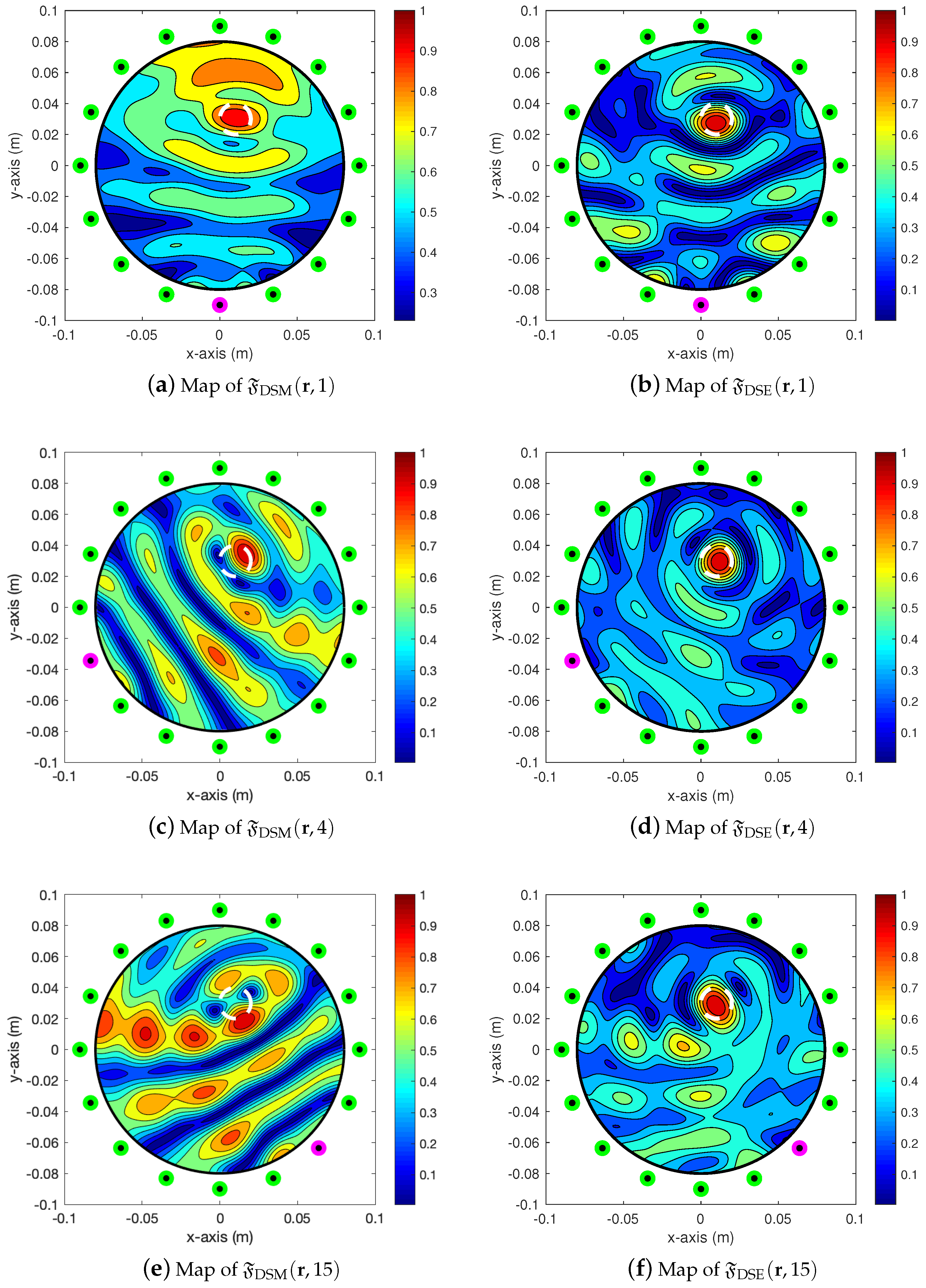
Example 1 (Simulation Result at $f=0.925 \mathrm{GHz}$).

Figure 2 shows the maps of ${\mathfrak{F}}_{DSM}(\mathbf{r},m)$ and ${\mathfrak{F}}_{DSE}(\mathbf{r},m)$ for $m=1,4,15$ at $f=0.925 \mathrm{GHz}$. As discussed above, the identified location of $\mathcal{D}$ via the map of ${\mathfrak{F}}_{DSM}(\mathbf{r},m)$ is not exactly in line with the actual location. Moreover, for each m, the identified locations of the anomaly obtained via ${\mathfrak{F}}_{DSM}(\mathbf{r},m)$ were different. This supports the observations discussed in Remark 1. In contrast, the identified location of $\mathcal{D}$ via the map of ${\mathfrak{F}}_{DSE}(\mathbf{r},m)$ is very close to the actual location and is independent from the location of the transmitter. Hence, we could assess the imaging performance of the ${\mathfrak{F}}_{DSE}(\mathbf{r},m)$ in relation to that of the ${\mathfrak{F}}_{DSM}(\mathbf{r},m)$.

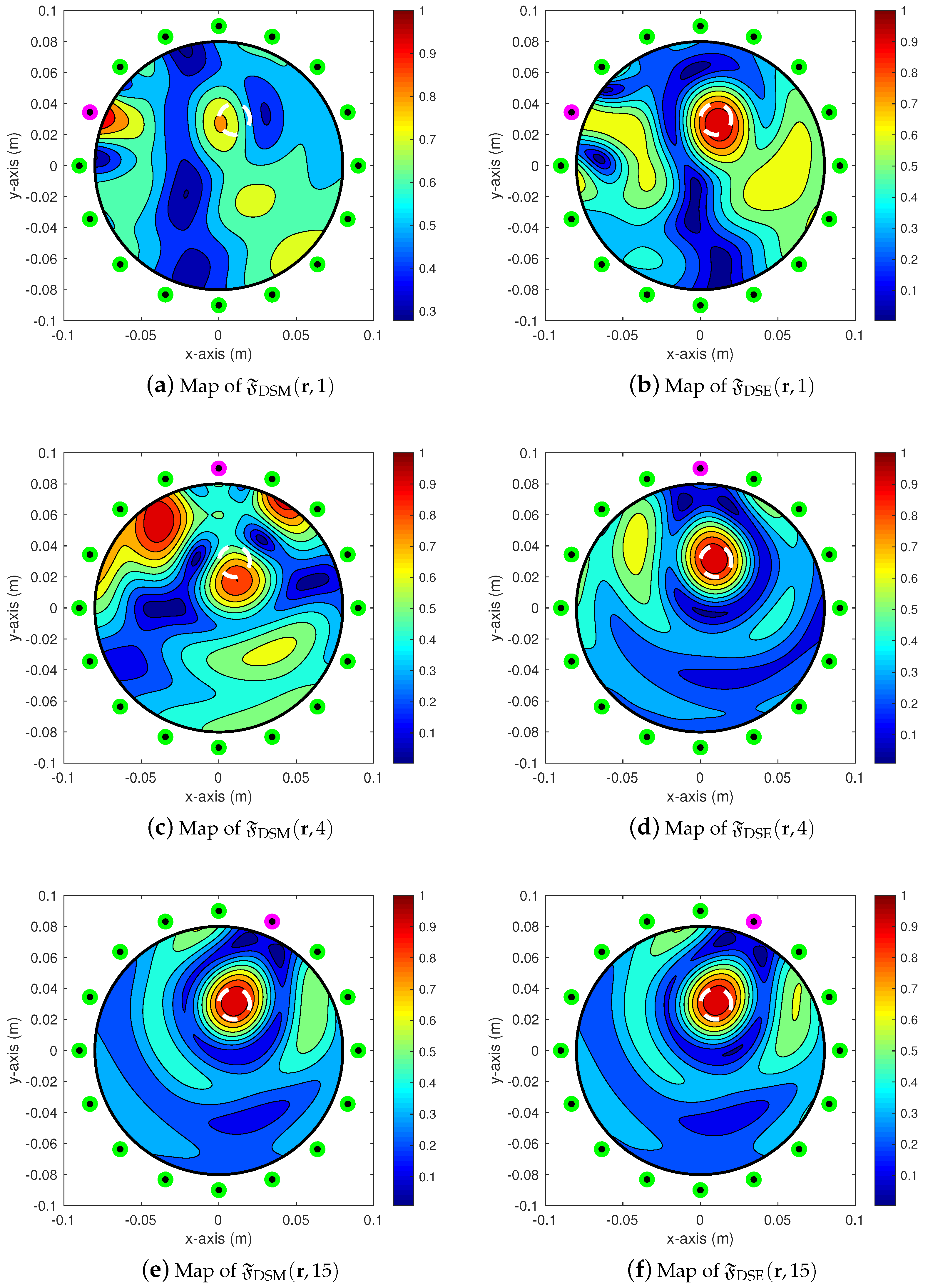
Example 2 (Simulation Result at $f=1.245 \mathrm{GHz}$).

Figure 3 shows the maps of ${\mathfrak{F}}_{DSM}(\mathbf{r},m)$ and ${\mathfrak{F}}_{DSE}(\mathbf{r},m)$ for $m=1,4,15$ at $f=1.245 \mathrm{GHz}$. When comparing these with those presented in Figure 2, it is clear that, even if the location of the transmitter is the same, the identified location of the anomaly is different. Meanwhile, almost the same result can be obtained via the map of ${\mathfrak{F}}_{DSM}(\mathbf{r},m)$ with a different frequency.

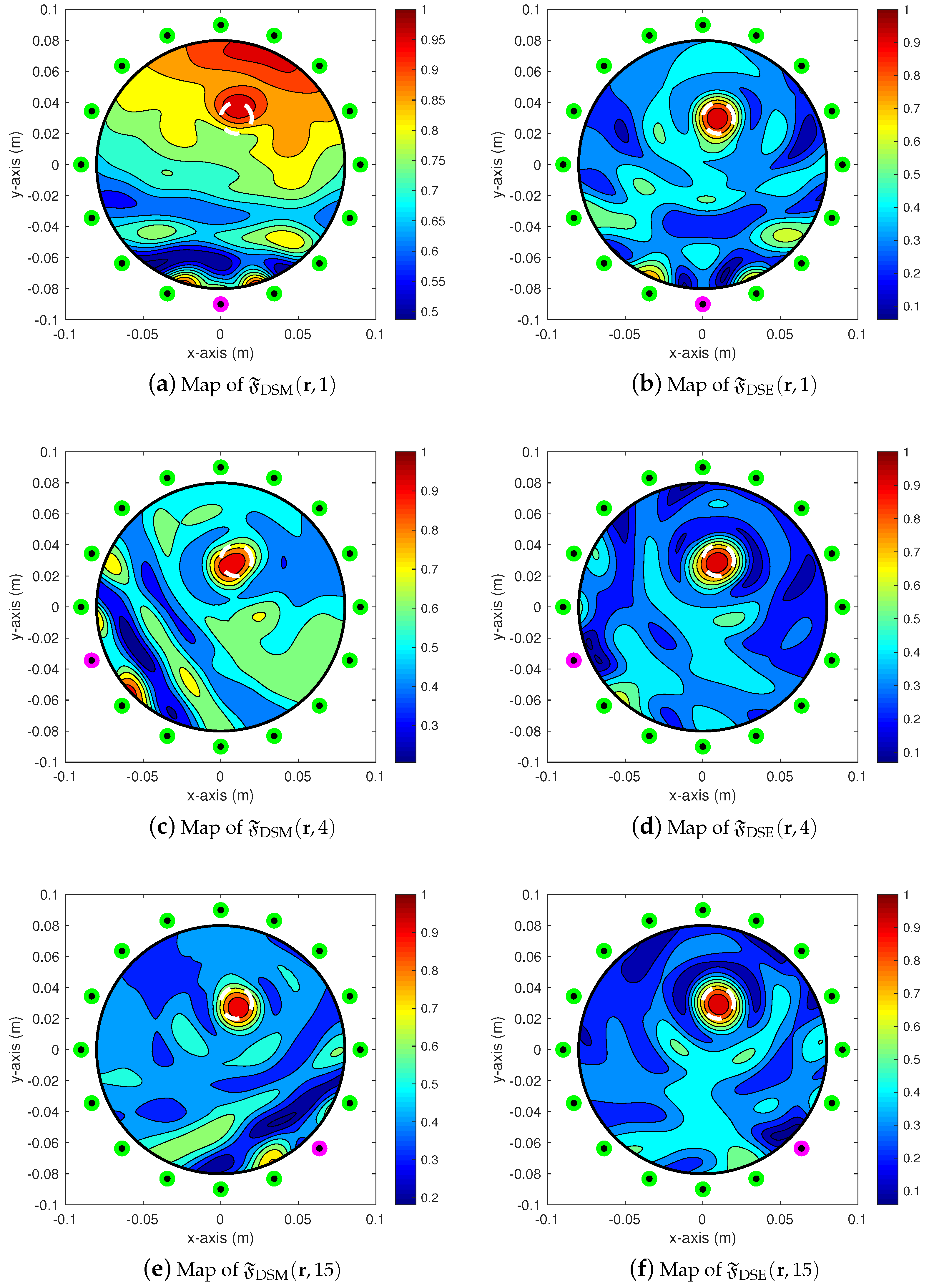
Example 3.

Figure 4 shows the maps of ${\mathfrak{F}}_{DSM}(\mathbf{r},m)$ and ${\mathfrak{F}}_{DSE}(\mathbf{r},m)$ for $m=6,9,10$ at $f=0.750 \mathrm{GHz}$. Notice that, although the distance between ${\mathbf{a}}_9$ and ${\mathbf{r}}_{★}$ is close, the identified location of $\mathcal{D}$ via the map of ${\mathfrak{F}}_{DSM}(\mathbf{r},9)$ is not accurate. Additionally, it is very hard and easy to identify the locations of $\mathcal{D}$ via the maps of ${\mathfrak{F}}_{DSM}(\mathbf{r},m)$ at $m=6$ and $m=10$, respectively. Thus, as we mentioned in Remark 1, the imaging performance of ${\mathfrak{F}}_{DSM}(\mathbf{r},m)$ significantly depends on the applied frequency and distance between the anomaly and the transmitter. Meanwhile, fortunately, the identified location of $\mathcal{D}$ via the map of ${\mathfrak{F}}_{DSE}(\mathbf{r},m)$ is very accurate to the actual location and is independent of the location of the transmitter. Hence, on the basis of the results in Figure 2 and Figure 3, we can conclude that imaging performance of ${\mathfrak{F}}_{DSE}(\mathbf{r},m)$ is better in relation to that of the ${\mathfrak{F}}_{DSM}(\mathbf{r},m)$.

Remark 3 (Discussion of Examples 1, 2, and 3).

Based on the results in Examples 1, 2, and 3, we can examine that the imaging performance of ${\mathfrak{F}}_{DSE}(\mathbf{r},m)$ is better than the one of ${\mathfrak{F}}_{DSM}(\mathbf{r},m)$. Moreover, as we observed ③ in Remark 1, the imaging performance of ${\mathfrak{F}}_{DSM}(\mathbf{r},m)$ is significantly dependent on the applied frequency. The imaging performance of ${\mathfrak{F}}_{DSE}(\mathbf{r},m)$ is also influenced by the applied frequency; however, recognization of the location of anomaly is very stable.

Example 4.

Figure 5 presents the results of the multi-frequency imaging of ${\mathfrak{F}}_{DSM}(\mathbf{r},m)$ and ${\mathfrak{F}}_{DSE}(\mathbf{r},m)$ for $m=1,4,15$ with a frequency band of $f\in [0.925\mathrm{G}\mathrm{Hz},1.245 \mathrm{GHz}]$. As was discussed in Remark 2, the identified location via the multi-frequency ${\mathfrak{F}}_{DSM}(\mathbf{r},m)$ is not accurate in the case of certain $m(=1)$, which means that there is no improvement to the imaging performance. However, the location of the anomaly can be identified clearly via the multi-frequency ${\mathfrak{F}}_{DSE}(\mathbf{r},m)$ because the magnitudes of several artifacts were reduced successfully.

Throughout the theoretical and simulation results, we can examine that established structures (5) and (6) prove the main research question about the coupling effect and provide answers to some phenomena that cannot be explained via previous research, and various imaging results of ${\mathfrak{F}}_{DSM}(\mathbf{r},m)$ successfully support the theoretical result. Moreover, the established structures (5) and (7) illustrate the improvement in imaging performance, and various imaging results of ${\mathfrak{F}}_{DSE}(\mathbf{r},m)$ show not only the verification of theoretical results but also the stability.

5. Concluding Remarks

In this contribution, two different indicator functions of DSM were introduced and designed for the fast identification of small anomalies from collected scattered-field S-parameters. To explain the influence of the coupling effect of traditional DSM and the improvement in the imaging performance of the designed indicator function, mathematical structures of traditional and designed indicator functions were analyzed by establishing a relationship between an infinite series of Bessel functions of integer order of the first kind and the antenna configuration.

We presented various simulation results from synthetic data computed by CST-STUDIO SUITE, and we examined that the imaging performance of traditional DSM is significantly influenced by the coupling effect, the designed indicator function is independent from the coupling effect and successfully improves the traditional one. Moreover, we confirmed that the designed DSM is very fast, stable, and effective for identifying small anomalies in microwave imaging. It is worth noticing that the identified shape of anomaly does not guarantee the accurate shape. Fortunately, it can be regarded as an initial guess and one can evolve it to retrieve a better shape via the iterative schemes. Therefore, it will be possible to examine that only a few iteration procedures are required, i.e., it will not require tremendous computations.

Here, we considered the two-dimensional problem. Following to [30], we expect that the designed indicator function can be extended to the more-realistic three-dimensional microwave imaging. It has been confirmed that DSM can be applied to the limited-aperture inverse scattering problem. The application of DSM in real-world limited-aperture microwave imaging and designing an improved DSM will be interesting research topics.

References

- Colton, D.; Kress, R. Inverse Acoustic and Electromagnetic Scattering Problems; Mathematics and Applications Series; Springer: New York, NY, USA, 1998. [Google Scholar]
- Ammari, H. Mathematical Modeling in Biomedical Imaging II: Optical, Ultrasound, and Opto-Acoustic Tomographies. In Lecture Notes in Mathematics; Springer: Berlin, Germany, 2011; Volume 2035. [Google Scholar]
- Chandra, R.; Johansson, A.J.; Gustafsson, M.; Tufvesson, F. A microwave imaging-based technique to localize an in-body RF source for biomedical applications. IEEE Trans. Biomed. Eng. 2015, 62, 1231–1241. [Google Scholar] [CrossRef] [PubMed]
- Haynes, M.; Stang, J.; Moghaddam, M. Real-time microwave imaging of differential temperature for thermal therapy monitoring. IEEE Trans. Biomed. Eng. 2014, 61, 1787–1797. [Google Scholar] [CrossRef] [PubMed] [Green Version]
- Bao, Q.; Yuan, S.; Guo, F. A new synthesis aperture-MUSIC algorithm for damage diagnosis on complex aircraft structures. Mech. Syst. Signal Proc. 2020, 136, 106491. [Google Scholar] [CrossRef]
- Foudazix, A.; Mirala, A.; Ghasr, M.T.; Donnell, K.M. Active microwave thermography for nondestructive evaluation of surface cracks in metal structures. IEEE Trans. Instrum. Meas. 2019, 68, 576–585. [Google Scholar] [CrossRef]
- Taillet, E.; Lataste, J.F.; Rivard, P.; Denis, A. Non-destructive evaluation of cracks in massive concrete using normal dc resistivity logging. NDT E Int. 2014, 63, 11–20. [Google Scholar] [CrossRef]
- Jung, S.H.; Cho, Y.S.; Park, R.S.; Kim, J.M.; Jung, H.K.; Chung, Y.S. High-resolution millimeter-wave ground-based SAR imaging via compressed sensing. IEEE Trans. Magn. 2018, 54, 9400504. [Google Scholar] [CrossRef]
- Liu, X.; Serhir, M.; Lambert, M. Detectability of underground electrical cables junction with a ground penetrating radar: Electromagnetic simulation and experimental measurements. Constr. Build. Mater. 2018, 158, 1099–1110. [Google Scholar] [CrossRef] [Green Version]
- Yang, S.T.; Ling, H. Application of compressive sensing to two-dimensional radar imaging using a frequency-scanned microstrip leaky wave antenna. J. Electromagn. Eng. Sci. 2017, 17, 113–119. [Google Scholar] [CrossRef] [Green Version]
- Kress, R. Inverse scattering from an open arc. Math. Meth. Appl. Sci. 1995, 18, 267–293. [Google Scholar] [CrossRef]
- Carpio, A.; Dimiduk, T.G.; Louër, F.L.; Rapún, M.L. When topological derivatives met regularized Gauss–Newton iterations in holographic 3D imaging. J. Comput. Phys. 2019, 388, 224–251. [Google Scholar] [CrossRef] [Green Version]
- Mojabi, P.; LoVetri, J. Microwave biomedical imaging using the multiplicative regularized Gauss-Newton inversion. IEEE Antennas Propag. Lett. 2009, 8, 645–648. [Google Scholar] [CrossRef]
- Colton, D.; Monk, P. The detection and monitoring of leukemia using electromagnetic waves: Numerical analysis. Inverse Prob. 1995, 11, 329–341. [Google Scholar] [CrossRef]
- Franchois, A.; Pichot, C. Microwave imaging-complex permittivity reconstruction with a Levenberg-Marquardt method. IEEE Trans. Antennas Propag. 1997, 45, 203–215. [Google Scholar] [CrossRef]
- Dorn, O.; Lesselier, D. Level set methods for inverse scattering. Inverse Prob. 2006, 22, R67–R131. [Google Scholar] [CrossRef] [Green Version]
- Ammari, H.; Garapon, P.; Jouve, F.; Kang, H.; Lim, M.; Yu, S. A new optimal control approach for the reconstruction of extended inclusions. SIAM J. Control Optim. 2013, 51, 1372–1394. [Google Scholar] [CrossRef] [Green Version]
- Park, W.K.; Lesselier, D. MUSIC-type imaging of a thin penetrable inclusion from its far-field multi-static response matrix. Inverse Prob. 2009, 25, 075002. [Google Scholar] [CrossRef]
- Park, W.K. Application of MUSIC algorithm in real-world microwave imaging of unknown anomalies from scattering matrix. Mech. Syst. Signal Proc. 2021, 153, 107501. [Google Scholar] [CrossRef]
- Park, W.K.; Kim, H.P.; Lee, K.J.; Son, S.H. MUSIC algorithm for location searching of dielectric anomalies from S-parameters using microwave imaging. J. Comput. Phys. 2017, 348, 259–270. [Google Scholar] [CrossRef]
- Park, W.K. Real-time microwave imaging of unknown anomalies via scattering matrix. Mech. Syst. Signal Proc. 2019, 118, 658–674. [Google Scholar] [CrossRef] [Green Version]
- Park, W.K. Fast imaging of thin, curve-like electromagnetic inhomogeneities without a priori information. Mathematics 2020, 8, 799. [Google Scholar] [CrossRef]
- Guo, J.; Yan, G.; Jin, J.; Hu, J. The factorization method for cracks in inhomogeneous media. Appl. Math. 2017, 62, 509–533. [Google Scholar] [CrossRef]
- Park, W.K. Experimental validation of the factorization method to microwave imaging. Results Phys. 2020, 17, 103071. [Google Scholar] [CrossRef]
- Louër, F.L.; Rapún, M.L. Topological sensitivity for solving inverse multiple scattering problems in 3D electromagnetism. Part I: One step method. SIAM J. Imag. Sci. 2017, 10, 1291–1321. [Google Scholar] [CrossRef]
- Yuan, H.; Bracq, G.; Lin, Q. Inverse acoustic scattering by solid obstacles: Topological sensitivity and its preliminary application. Inverse Probl. Sci. Eng. 2016, 24, 92–126. [Google Scholar] [CrossRef]
- Agarwal, K.; Chen, X.; Zhong, Y. A multipole-expansion based linear sampling method for solving inverse scattering problems. Opt. Express 2010, 18, 6366–6381. [Google Scholar] [CrossRef]
- Aram, M.G.; Haghparast, M.; Abrishamian, M.S.; Mirtaheri, A. Comparison of imaging quality between linear sampling method and time reversal in microwave imaging problems. Inverse Probl. Sci. Eng. 2016, 24, 1347–1363. [Google Scholar] [CrossRef]
- Ito, K.; Jin, B.; Zou, J. A direct sampling method to an inverse medium scattering problem. Inverse Prob. 2012, 28, 025003. [Google Scholar] [CrossRef]
- Ito, K.; Jin, B.; Zou, J. A direct sampling method for inverse electromagnetic medium scattering. Inverse Prob. 2013, 29, 095018. [Google Scholar] [CrossRef] [Green Version]
- Kang, S.; Lambert, M.; Park, W.K. Direct sampling method for imaging small dielectric inhomogeneities: Analysis and improvement. Inverse Prob. 2018, 34, 095005. [Google Scholar] [CrossRef] [Green Version]
- Kang, S.; Lambert, M.; Ahn, C.Y.; Ha, T.; Park, W.K. Single- and multi-frequency direct sampling methods in limited-aperture inverse scattering problem. IEEE Access 2020, 8, 121637–121649. [Google Scholar] [CrossRef]
- Park, W.K. Detection of small inhomogeneities via direct sampling method in transverse electric polarization. Appl. Math. Lett. 2018, 79, 169–175. [Google Scholar] [CrossRef] [Green Version]
- Ahn, C.Y.; Ha, T.; Park, W.K. Direct sampling method for identifying magnetic inhomogeneities in limited-aperture inverse scattering problem. Comput. Math. Appl. 2020, 80, 2811–2829. [Google Scholar] [CrossRef]
- Park, W.K. Direct sampling method for retrieving small perfectly conducting cracks. J. Comput. Phys. 2018, 373, 648–661. [Google Scholar] [CrossRef] [Green Version]
- Chow, Y.T.; Ito, K.; Liu, K.; Zou, J. Direct sampling method for diffusive optical tomography. SIAM J. Sci. Comput. 2015, 37, A1658–A1684. [Google Scholar] [CrossRef]
- Chow, Y.T.; Ito, K.; Zou, J. A direct sampling method for electrical impedance tomography. Inverse Prob. 2014, 30, 095003. [Google Scholar] [CrossRef] [Green Version]
- Liu, K.; Xu, Y.; Zou, J. A multilevel sampling method for detecting sources in a stratified ocean waveguide. J. Comput. Appl. Math. 2017, 309, 95–110. [Google Scholar] [CrossRef] [Green Version]
- Ji, X.; Liu, X.; Zhang, B. Phaseless inverse source scattering problem: Phase retrieval, uniqueness and direct sampling methods. J. Comput. Phys. X 2019, 1, 100003. [Google Scholar] [CrossRef]
- Kang, S.; Lambert, M.; Park, W.K. Analysis and improvement of direct sampling method in the mono-static configuration. IEEE Geosci. Remote Sens. Lett. 2019, 16, 1721–1725. [Google Scholar] [CrossRef]
- Park, W.K. Direct sampling method for anomaly imaging from scattering parameter. Appl. Math. Lett. 2018, 81, 63–71. [Google Scholar] [CrossRef] [Green Version]
- Son, S.H.; Lee, K.J.; Park, W.K. Application and analysis of direct sampling method in real-world microwave imaging. Appl. Math. Lett. 2019, 96, 47–53. [Google Scholar] [CrossRef] [Green Version]
- Park, W.K. Negative result of multi-frequency direct sampling method in microwave imaging. Results Phys. 2019, 12, 859–860. [Google Scholar] [CrossRef]
- Slaney, M.; Kak, A.C.; Larsen, L.E. Limitations of imaging with first-order diffraction tomography. IEEE Trans. Microwave Theory Tech. 1984, 32, 860–874. [Google Scholar] [CrossRef] [Green Version]
- Ammari, H.; Garnier, J.; Kang, H.; Park, W.K.; Sølna, K. Imaging schemes for perfectly conducting cracks. SIAM J. Appl. Math. 2011, 71, 68–91. [Google Scholar] [CrossRef] [Green Version]
- Park, W.K. Improvement of direct sampling method in transverse electric polarization. Appl. Math. Lett. 2019, 88, 209–215. [Google Scholar] [CrossRef]
Figure 1.
Illustration of the simulation configuration.
Figure 2.
Maps of and at . White-colored dashed line describes the .
Figure 3.
Figure 4.
Figure 5.
Multi-frequency imaging of and . White-colored dashed line describes the .
Publisher’s Note: MDPI stays neutral with regard to jurisdictional claims in published maps and institutional affiliations. |
© 2021 by the author. Licensee MDPI, Basel, Switzerland. This article is an open access article distributed under the terms and conditions of the Creative Commons Attribution (CC BY) license (https://creativecommons.org/licenses/by/4.0/).
Share and Cite
MDPI and ACS Style
Park, W.-K. Theoretical Identification of Coupling Effect and Performance Analysis of Single-Source Direct Sampling Method. Mathematics 2021, 9, 1065. https://doi.org/10.3390/math9091065
AMA Style
Park W-K. Theoretical Identification of Coupling Effect and Performance Analysis of Single-Source Direct Sampling Method. Mathematics. 2021; 9(9):1065. https://doi.org/10.3390/math9091065
Chicago/Turabian StylePark, Won-Kwang. 2021. "Theoretical Identification of Coupling Effect and Performance Analysis of Single-Source Direct Sampling Method" Mathematics 9, no. 9: 1065. https://doi.org/10.3390/math9091065
Note that from the first issue of 2016, this journal uses article numbers instead of page numbers. See further details here.