An Advanced Angular Velocity Error Prediction Horizon Self-Tuning Nonlinear Model Predictive Speed Control Strategy for PMSM System

Abstract

In nonlinear model predictive control (NMPC), higher accuracy can be obtained with a shorter prediction horizon in steady-state, better dynamics can be obtained with a longer prediction horizon in a transient state, and calculation burden is proportional to the prediction horizon which is usually pre-selected as a constant according to dynamics of the system with NMPC. The minimum calculation and prediction accuracy are hard to ensure for all operating states. This can be improved by an online changing prediction horizon. A nonlinear model predictive speed control (NMPSC) with advanced angular velocity error (AAVE) prediction horizon self-tuning method has been proposed in which the prediction horizon is improved as a discrete-time integer variable and can be adjusted during each sampling period. A permanent magnet synchronous motor (PMSM) rotor position control system with the proposed strategy is accomplished. Tracking performances including rotor position Integral of Time-weighted Absolute value of the Error (ITAE), the maximal delay time, and static error are improved about 15.033%, 23.077%, and 10.294% respectively comparing with the conventional NMPSC strategy with a certain prediction horizon. Better disturbance resisting performance, lower weighting factor sensitivities, and higher servo stiffness are achieved. Simulation and experimental results are given to demonstrate the effectiveness and correctness.

1. Introduction

Permanent magnet synchronous motor (PMSM) is frequently used in industry due to high level of power density, efficiency, and torque-ampere ratio with low weight and volume [1]. The proportional-integral (PI) controller is usually used in the PMSM control system to control motor speed and stator currents to obtain desired dynamic and performance. Many improved control strategies are presented to satisfy different criteria, such as 2-degree-of-freedom (2-DoF) control, internal model control (IMC), active disturbance rejection control (ADRC), and model predictive control (MPC). Two controllers are adopted in the 2-DoF control to adjust and decouple dynamic and disturbance resisting performance [2]. A model of the controlled plant is added into the structure of IMC to make the system operate in an open-loop manner to resist disturbance [3]. An extended state observer (ESO) is introduced into the ADRC strategy, and all disturbances are estimated and compensated [4]. The above control strategies can meet the basic requirements of the PMSM system. MPC strategy has been highlighted in recent years due to better dynamics, easier understanding, and handling, and has been widely applied in motor driving and power electronic realm [5]. MPC can be divided as continuous-control-set MPC (CCS-MPC) and finite-control-set MPC (FCS-MPC) [6]. Since modulation is adopted in the CCS-MPC, fewer ripple and switching losses can be obtained compared with FCS-MPC with variable switching frequency [7]. But the prediction horizon in CCS-MPC is hard to be adjusted due to the limitation of the voltage function generation process. MPC belongs to a short prediction horizon method covering only one sampling period. The MPC in the PMSM system can be divided into model predictive current control (MPCC), model predictive speed control (MPSC), and model predictive torque control (MPTC) according to the primary control objective [8,9,10]. A voltage smoother in [11] and an integral sliding mode disturbance observer in [12] are combined with the MPSC respectively to enhance control performances of speed or angular velocity.

Aiming at high stability and tracking performances, some improvements such as Sequential MPC (SMPC), Parallel MPC (PMPC), and NMPC are proposed to prolong the prediction horizon to several sampling periods [13,14], and the prediction horizon of Nonlinear predictive control (NPC) is extended to thousands of sampling periods which are within the Shannon upper bound [15]. These are called long prediction horizon methods.

NPC is a generalized nonlinear method linearized by Lie derivation. It is usually combined with an advanced algorithm to build a nonlinear object model and to design the controller [16].

In SMPC, the cost function is split into several parts according to the multiple controlled objectives or variables [17]. In PMPC, a switching vector intersection method is inserted into the MPTC structure to select the optimal vector to obtain better robustness and dynamics [18]. A compensatory block of the three-phase inverter is inserted before MPC processes, the input state variables of SMPC and PMPC are at time k + 1 [19]. As a result, the predictive variables in the discrete-time model are at time k + 2 [20]. Due to the divided cost functions, the calculation time is increased because of the calculation of the cost function values and the selection of vectors in each step, and the number of controlled objectives is restricted by the number of vectors of the switching table. This can be solved by adding a group of extra vectors [21].

SMPC and PMPC cover two sampling periods, which improves system performances finitely. An accumulating type nonlinear cost function is presented and used in NMPC to prolong the prediction horizon [22]. Some extra weighting factors are added to the cost function to enhance convergence of the system [23], and an improved extended prediction horizon method for NMPC is proposed under the condition of limited calculation burdens [24]. The stability of the extended prediction horizon is verified in theory [25]. A kind of adaptive dynamic programming (ADP) algorithm is combined with the NMPC to improve the robustness and dynamics [26]. NMPC is used in many applications of power systems and power electronic realms. The extended prediction horizons in the traditional methods are fixed. It does not benefit all operating states, for example, the calculation burden and prediction error are increased heavily in steady-state, and hence the performances are also affected. An extended prediction self-adaptive control (EPSAC) [27] and Nonlinear EPSAC (NEPSAC) [28] to NMPC strategy are proposed in [29] to auto-tune the sampling period and the maximum prediction horizon to enhance robustness and dynamics of different systems.

MPSC strategy and NMPC structure are combined as so-called NMPSC. An NMPSC with AAVE prediction horizon self-tuning method is proposed in this paper and applied to the PMSM rotor position system. The prediction horizon is improved as a discrete-time integral variable which can be adjusted in every sampling period to improve tracking accuracy. Performance comparisons including rotor position error, servo stiffness, and weighting factor sensitivities are conducted between the proposed method and the conventional NMPSC without any prediction horizon self-tuning method. According to the simulation and experimental results, servo stiffness, weighting factor sensitivities, and ITAEs are improved effectively.

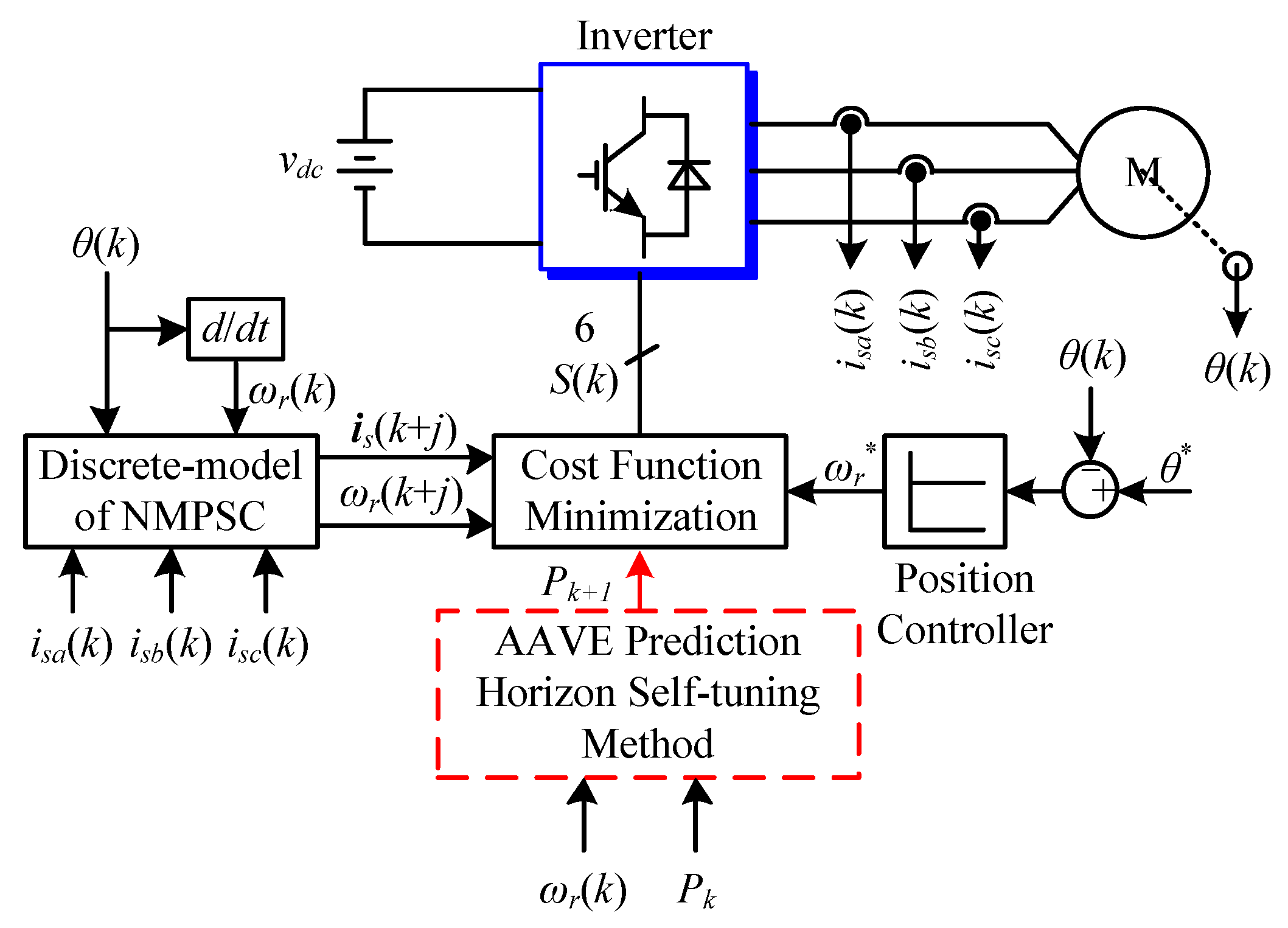
2. PMSM Model and NMPSC Strategy

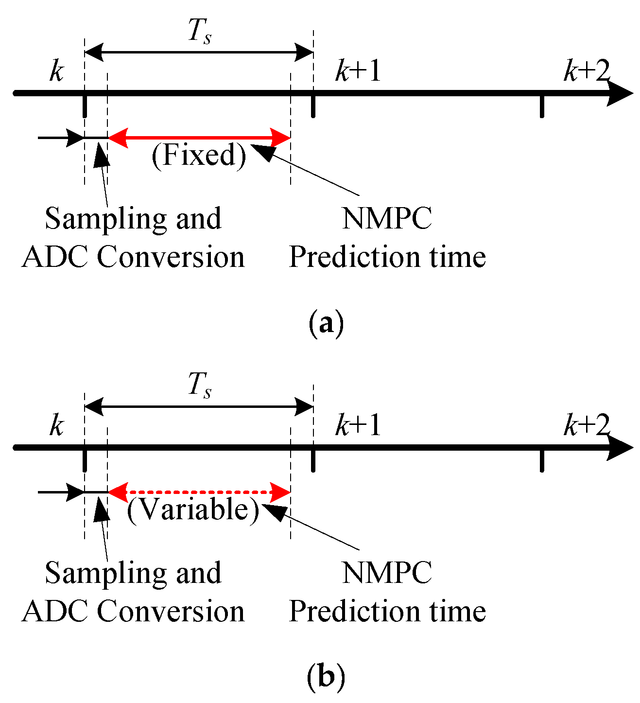
2.1. Problem Description

Stability and rapidity are the main indicators of the PMSM control system. High accuracy and low operation burden of the system are also required during the steady-state [13].

Time delay has to be considered for the selected switching signal, which results that the output cannot be output in time in the digital control system [10]. NMPC predicts the variables at time k + j based on the sampled signals and selected prediction horizon by repetitive predictive processes. Figure 1 shows the time flows of two NMPC strategies. The prediction calculation time of the conventional NMPC is constant in solid line as shown in Figure 1a and it is adjustable in variable prediction horizon NMPC in dash-line as shown in Figure 1b. The delay time is not fixed in the variable prediction horizon NMPC. Prediction processes and cost function calculation processes are two main parts of the prediction time slot. Since the number of voltage vectors is pre-selected, the prediction time is changed with the number of prediction processes which equals the prediction horizon.

The control performance of NMPC is related to the prediction horizon. For the transient state, a longer prediction horizon is usually required to achieve better dynamic performances to resist disturbance. This induces a heavier calculation burden and lowers accuracy due to longer calculation time and more neglected sampling points [24]. As for the steady-state, a shorter prediction horizon with better accuracy and a lighter calculation burden is required to enhance steady performances and to decrease static error. Therefore, the prediction horizon should be adjusted for different operating states to realize optimal operating performance.

2.2. Discrete-Time Model

The state functions of the PMSM model can be expressed based on the two-phase synchronized rotation reference frame. The functions including the stator voltage v_s, flux linkage ψ_s and electromagnetic torque T_e for the Surface PMSM (SPMSM) are expressed as:

$$\{\begin{array}{c}{v}_{sd}=R_s{i}_{sd}+L_s\frac{d{i}_{sd}}{dt}-L_s{\omega }_r{i}_{sq}\\ v_{sq}=R_s{i}_{sq}+L_s\frac{d{i}_{sq}}{dt}+L_s{\omega }_r{i}_{sd}+{\psi }_m{\omega }_r\end{array}$$

(1)

$$\{\begin{array}{c}{\psi }_{sd}=L_s{i}_{sd}+{\psi }_m\\ {\psi }_{sq}=L_s{i}_{sq}\end{array}$$

(2)

$$T_e=\frac{3}{2}p{\psi }_m{i}_{sq}$$

(3)

and the electrical angular velocity ω_r can be described by the equation as:

$$\frac{d{\omega }_r}{dt}=\frac{p}{J}\left(T_e-T_L\right)-\frac{B}{J}{\omega }_r$$

(4)

where subscripts d and q mean that the components of variables locate in the d-axis and q-axis respectively, such as i_sd and i_sq are stator current components on the d-axis and q-axis respectively. Moreover, L_s is stator self-inductance which is satisfying L_s = L_sq = L_sd for SPMSM, T_L is load torque, R_s is stator resistance, p is the number of pole pairs, J is rotor inertia, B is friction coefficient and ψ_m is rotor flux magnitude.

Combining Equations (1) to (4), the space state equation of PMSM can be expressed as:

$$h\left(\mathit{x},\mathit{u}\right)=\frac{d\mathit{x}}{dt}$$

(5)

where

$$\mathit{x}={\left[\begin{array}{ccc}{i}_{sd}& i_{sq}& {\omega }_r\end{array}\right]}^{\mathrm{T}}$$

(6)

$$\mathit{u}={\left[\begin{array}{cc}{v}_{sd}& v_{sq}\end{array}\right]}^{\mathrm{T}}$$

(7)

$$h\left(\mathit{x},\mathit{u}\right)=\left[\begin{array}{c}-\frac{R_s}{L_s}{i}_{sd}+{\omega }_r{i}_{sq}+\frac{1}{L_s}{v}_{sd}\\ -\frac{R_s}{L_s}{i}_{sq}-{\omega }_r{i}_{sd}-\frac{{\psi }_m}{L_s}{\omega }_r+\frac{1}{L_s}{v}_{sq}\\ \frac{3p^2{\psi }_m}{2J}{i}_{sq}-\frac{B}{J}{\omega }_r\end{array}\right]$$

(8)

The two-step Euler interpolation method including predicting step x_p(k + 1) and correcting step x(k + 1) is used to predict and discretize the model based on a sampling period T_s, and the expressions are [5]:

$$\{\begin{array}{c}{\mathit{x}}_p\left(k+1\right)=\mathit{x}\left(k\right)+T_{s}h\left(\mathit{x}\left(k\right),\mathit{u}\left(k\right)\right)\\ \mathit{x}\left(k+1\right)=\mathit{x}\left(k\right)+\frac{T_s}{2}\left(h\left(\mathit{x}\left(k\right),\mathit{u}\left(k\right)\right)+h\left({\mathit{x}}_p\left(k+1\right),\mathit{u}\left(k\right)\right)\right)\end{array}$$

(9)

2.3. NMPSC Strategy

The typical cost function for NMPC is [29]:

$$J(\mathit{U})={{\displaystyle \sum _{j=N_1}^{N_2}\left[r(t+k|t)-y(t+k|t)\right]}}^2$$

(10)

where N₁ and N₂ are the minimum and the maximum prediction horizons which are constant values. The basic idea of the method is to calculate a sequence of future control signals to minimize a cost function defined over a prediction horizon. For the PMSM control system, N₁ can be selected as 1 which meets the prediction horizon in MPSC, and N₂ can be selected according to the Shannon sampling principle and calculation burden of the processor.

Speed reference tracking and torque ampere optimization are two main objectives in the PMSM system, therefore, the cost function for NMPSC can be determined as [5]:

$$G={\displaystyle \sum _{j=1}^{N_2}\left[{\lambda }_{\omega }{\left({\omega }_r\left(k+j\right)-{\omega }_r^{*}\right)}^2+{\lambda }_i{\left(i_{sd}\left(k+j\right)\right)}^2\right]}$$

(11)

where λ_ω and λ_i are two weighting factors reflecting the importance of the objectives. The reference tracking is realized by the first term of the cost function. i_sq is related to ω_r according to the discrete-time model in Equations (4) and (5), as a result, it can be controlled by the first term at the same time. The torque ampere optimization objective is realized by the second term of the cost function.

To enhance convergence of the system, a group of weighting factors Q_j converging to zero are added into the cost function, Equation (11), as:

$$G={\displaystyle \sum _{j=1}^{N_2}{Q}_j\left[{\lambda }_{\omega }{\left({\omega }_r\left(k+j\right)-{\omega }_r^{*}\right)}^2+{\lambda }_i{\left(i_{sd}\left(k+j\right)\right)}^2\right]}$$

(12)

and the weighting factor Q_j has a common tuning function:

$$Q_j=\frac{1}{1+j}$$

(13)

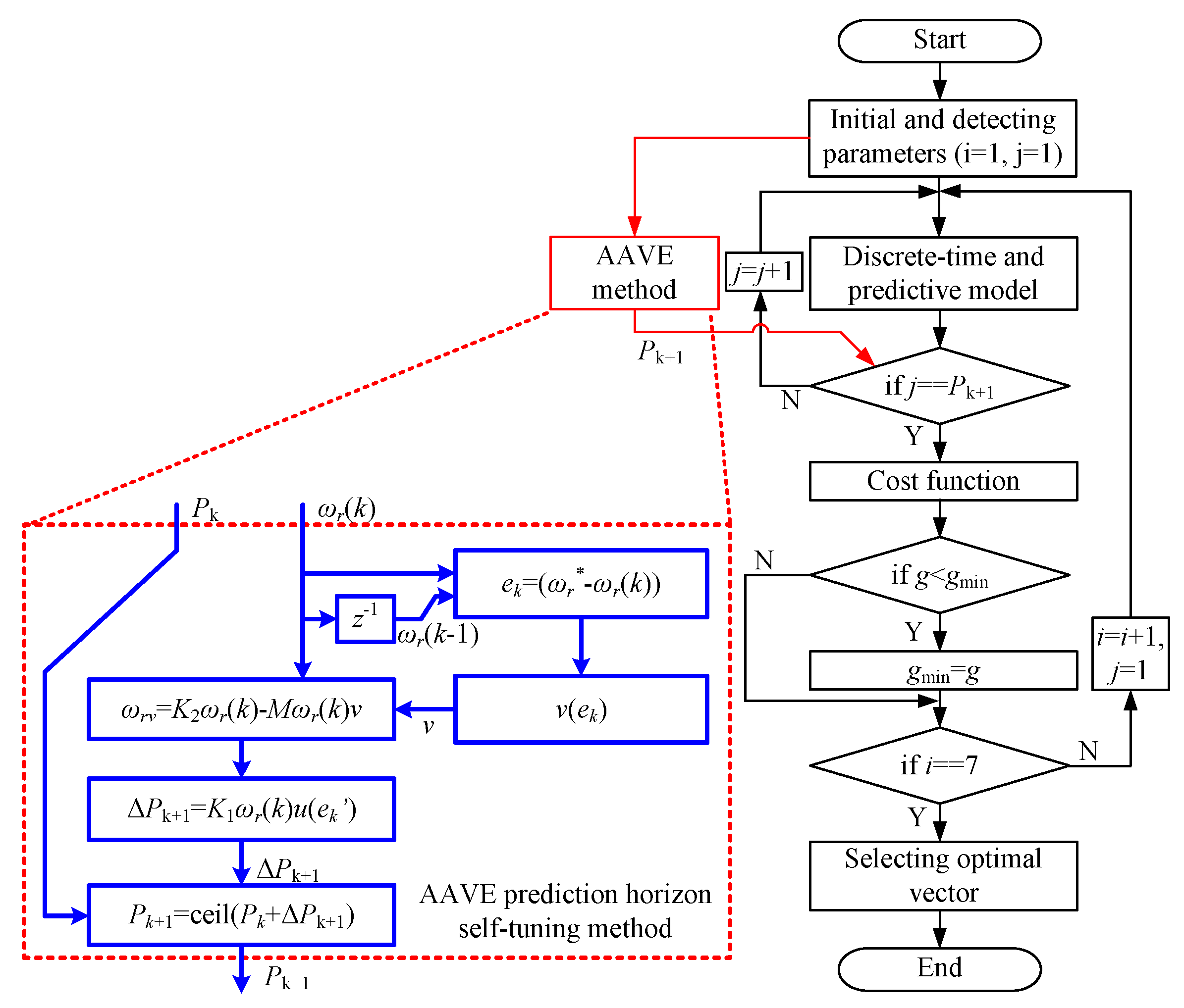
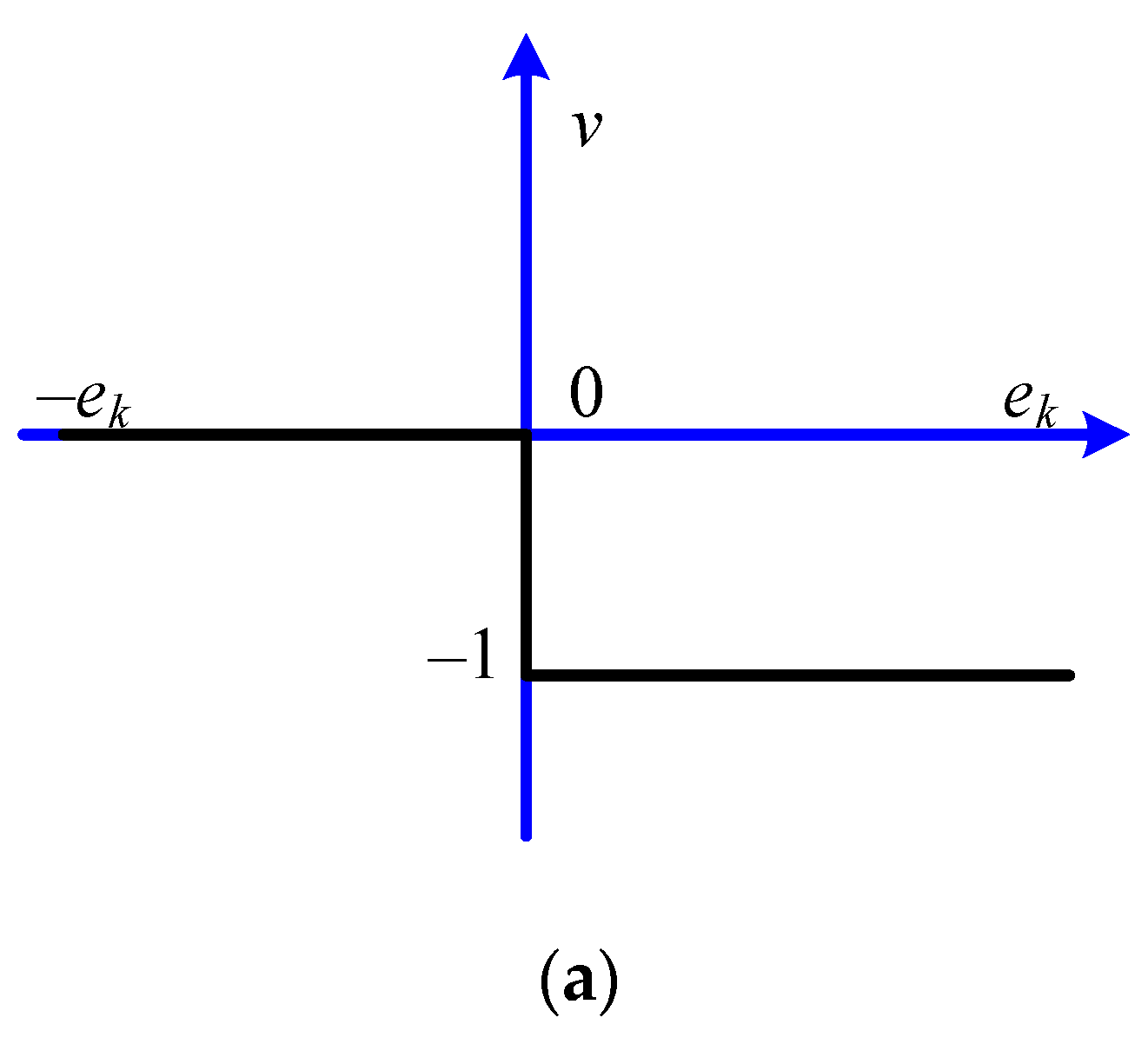
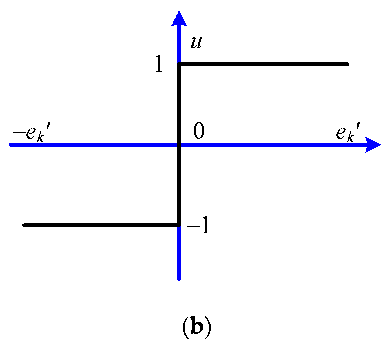
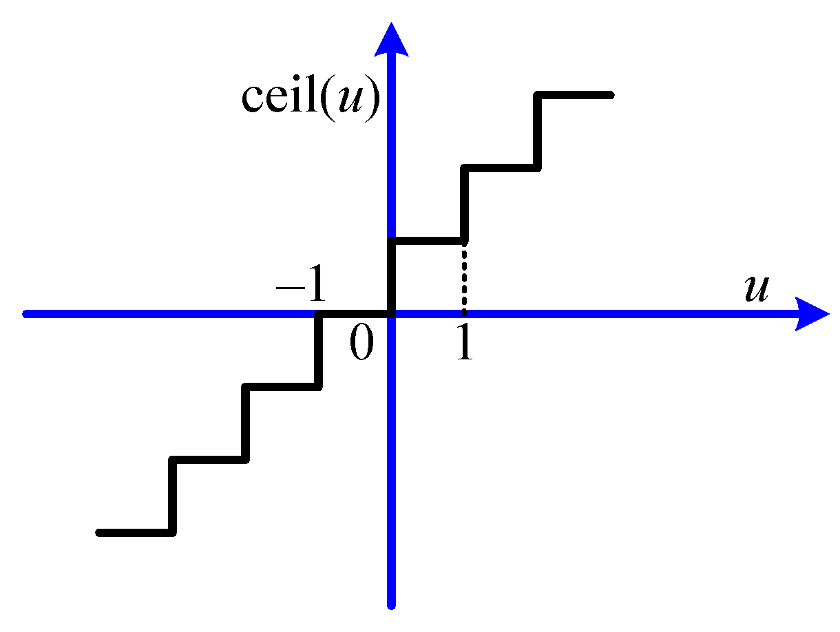
3. Proposed AAVE Method

Redefining the prediction horizon N₂ in Equation (12) as a positive discrete-time integral variable P_k+1, the cost function is improved as:

$$G={\displaystyle \sum _{j=1}^{P_{k+1}}{Q}_j\left[{\lambda }_{\omega }{\left({\omega }_r\left(k+j\right)-{\omega }_r^{*}\right)}^2+{\lambda }_i{\left(i_{sd}\left(k+j\right)\right)}^2\right]}$$

(14)

where ω_r* is angular velocity reference.

There are two fundamental objectives: (1) to ensure that the angular velocity reference ω_r* is tracked, and (2) to guarantee that a virtual reference ω_rv* is generated and to modify the prediction horizon to the optimal value automatically. The flowchart of the proposed method is shown in Figure 2, where i and j are two cyclic variables, i is used to make sure that all voltage vectors are fully considered, and j is used to judge whether the prediction horizon accumulating processes are accomplished.

• Measurement and detection;

The angular velocity ω_r is measured by an encoder, and the prediction horizon P_k at the last sampling period is stored in the register for the calculating process at the k-th sampling period.

2.

Virtual reference and step generation;

Once the current angular velocity ω_r is different from that of the previous sampling period, the virtual reference ω_rv needs to be redefined automatically during each sampling period so that it can converge to a new optimal prediction horizon when there is an abrupt change in the system.

The virtual reference ω_rv and the step increment ΔP_k+1 of the prediction horizon at k + 1-th sampling period can be calculated as:

$${\omega }_{rv}=K_2{\omega }_r\left(k\right)+M{\omega }_r\left(k\right)v$$

(15)

and

$$\mathsf{\Delta }{P}_{k+1}=K_1{\omega }_r\left(k\right)u$$

(16)

where

$$v=-\frac{1}{2}-\frac{1}{2}\mathrm{sign}\left(e_k\right)$$

(17)

$$e_k={\omega }_r^{*}-{\omega }_r\left(k\right)$$

(18)

$$u=\mathrm{sign}\left({e^{\prime }}_k\right)$$

(19)

$${e^{\prime }}_k={\omega }_{rv}-{\omega }_r\left(k\right)$$

(20)

and K₁, K_2, and M are coefficients to ensure the same order of magnitudes of ω_rv as that of ω_r and the limited change of the prediction horizon, and a constraint as 2K₂ < M < ∞ should be satisfied to obtain a determined sign of the virtual reference. K₁, K₂, and M are selected as 0.05, 1, and 2 respectively in the strategy. The functions v and u are shown in Figure 3. The virtual reference ω_rv and prediction horizon P_k+1 have positive slopes when the angular velocity error e_k at the k-th sampling period increases and vice versa.

• Prediction horizon calculation and range judgment.

The prediction horizon at k + 1-th sampling period P_k+1 can be calculated as follow:

$$P_{k+1}=P_k+\mathsf{\Delta }{P}_{k+1}$$

(21)

According to Equation (11), P_k+1 should be integral between 1 and N₂, and the result in (21) should be handled as follow:

$$P_{k+1}=\{\begin{array}{ccc}{N}_2& if& \mathrm{ceil}\left(P_k+\mathsf{\Delta }{P}_{k+1}\right)>N_2\\ \mathrm{ceil}\left(P_k+\mathsf{\Delta }{P}_{k+1}\right)& if& N_2\ge \mathrm{ceil}\left(P_k+\mathsf{\Delta }{P}_{k+1}\right)>1\\ 1& if& \mathrm{ceil}\left(P_k+\mathsf{\Delta }{P}_{k+1}\right)\le 1\end{array}$$

(22)

where the function ceil (.) is a value round-up function that makes sure that the prediction horizon is an integral value as shown in Figure 4.

The resulted P_k+1 from Equation (22) is brought into Equation (14) to form the cost function. After all of the voltage vectors are evaluated in the cost function, the voltage vector with the minimum cost function value can be selected as the optimal vector.

According to the conventional NMPSC cost function in Equation (12), usually N₁ = 1, N₂ is a fixed value that satisfies the stability condition in [30] and maintains constant during the operation of the system. For the proposed method, N₂ is also selected from the range to ensure stability, but the prediction horizon P_k+1 is adjusted within the range to achieve optimum performances in every sampling period.

4. Simulation Results and Analysis

The structure diagram of NMPSC with AAVE prediction horizon self-tuning method on a PMSM rotor position system is shown in Figure 5. A simulation environment has been built in the MATLAB/Simulink software according to the structure. The weighting factors λ_ω and λ_i are selected by the branch and bound algorithm as 1 and 0.5 respectively [5]. The sampling frequency f_s and the maximum prediction horizon N₂ are selected as 10 kHz and 100. Some important parameters of PMSM are listed in

Table 1. Main parameters of PMSM.

Symbol	Quantity	Value
Rs	Stator resistance	2.875 Ω
Ls	Stator self-inductance	0.835 mH
J	Rotor inertia	0.0008 kg∙m2
B	Friction coefficient	0.0008 N∙m·s
p	The number of pole pairs	4
ψm	Flux magnitude due to rotor magnets	0.175 Wb
nn	Rated speed	3000 rpm
fn	Rated frequency	200 Hz
Pn	Rated power	1 kW
Vn	Rated voltage	380 V
In	Rate current	3.65 A
η	Shaft driving efficiency	82.6%

.

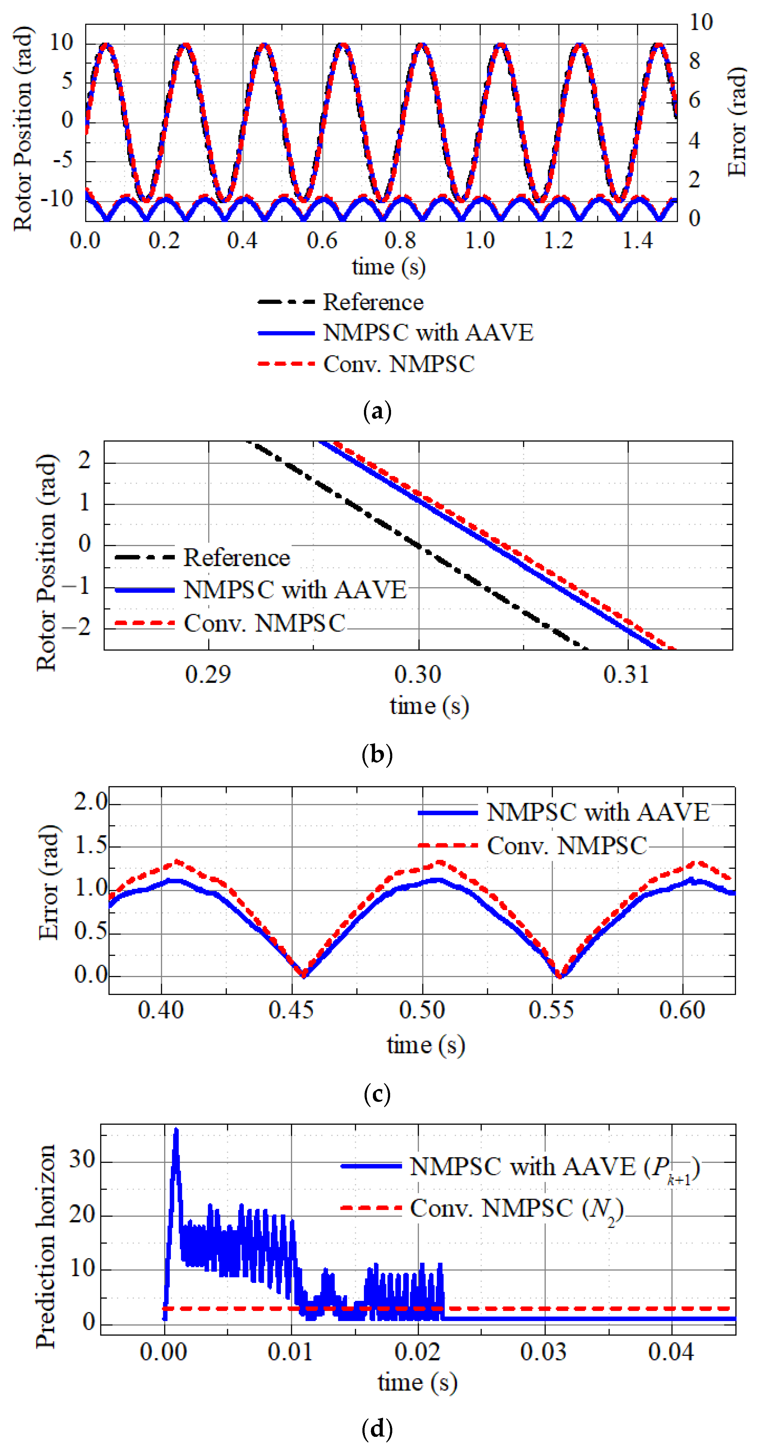
4.1. Tracking Performance Analysis

The rotor position reference θ* is given by a sinusoidal signal with amplitude 10, 5 Hz, and zero initial phases. The reference, rotor position, and error waveforms of the NMPSC with AAVE prediction horizon self-tuning method and the conventional NMPSC with constant prediction horizon value are shown in Figure 6. The left y-axis in Figure 6a reflects rotor position and rotor position waves are all sinusoidal, and the right y-axis in Figure 6a reflects rotor position error and the rotor position error waves have doubled frequency comparing with rotor position waves. The part enlarged waves including both rotor positions and errors are shown in Figure 6b,c. Figure 6b,c shows that the rotor position in the NMPSC with AAVE prediction horizon self-tuning method can track the reference with a delay time of about 4ms, and its maximum static error is about 1rad. As for the conventional NMPSC strategy, they are 4.2 ms and 1.2 rad. During normal operation, the maximal error occurs near the crossing zero points.

The prediction horizon waves at starting operation stage are shown in Figure 6d. Comparing with the fixed prediction horizon in the conventional strategy, the P_k+1 of the proposed method is changed with the errors. Around 22 ms, the prediction horizons are converged to 1 when the actual rotor position signal tracks the reference successfully. Because the delay errors, which exist in measurement, calculation, transmission, and action processes of the digital system, are neglected in the simulation environment, the ideal errors are not large enough to trigger the AAVE prediction horizon self-tuning method during normal tracking processes.

The converter efficiency is also tested in simulations. It is about 0.9918 for the proposed method and 0.98 for conventional strategies. The increment is about 1.204%.

ITAE is a comprehensive index defining the absolute value of accumulating error during the whole operating process which can be expressed as:

$$ITAE={\displaystyle {\int }_0^{\infty }\left|e\left(t\right)\right|tdt}$$

(23)

The rotor position ITAE, speed ITAE of the NMPSC with the proposed method, and the conventional NMPSC within 1.5s are listed in

Table 2. Performance comparison within 1.5 s.

Control Performances	NMPSC with the Proposed Method	Conventional NMPSC
Rotor position ITAE	0.7771	0.9499
Speed ITAE	7.931	10.73

. The lowest ITAE values are obtained for the proposed method due to decreased errors at the start operation state mainly.

Two ramp signals with slope ±200 rad/s are adopted as rotor position references to compare performance in the same speed region. Simulation results are shown in Figure 7. It is shown that rotor position waves of two strategies can track the references with similar delay times, and speeds are around ±95 rpm respectively.

A 3 N∙m load torque is added at 0.3 s, the torque currents (q-axis) are increased to resist load torque, and the current increasing process of the proposed strategy is slightly shorter than the conventional NMPSC.

Rotor position and speed ITAEs within 0.8 s are listed in

Table 3. Ramp reference performance comparisons within 0.8 s.

Control Strategies	Speed Direction	NMPSC with the Proposed Method	Conventional NMPSC
NMPSC with the proposed method	Positive	0.2241	1.982
	Negative	0.2171	1.718
Conventional NMPSC	Positive	0.232	2.15
	Negative	0.213	1.504

, ITAE values can be decreased by about 3.53% for the proposed strategy and increased by about 1.88% when the speed direction is negative.

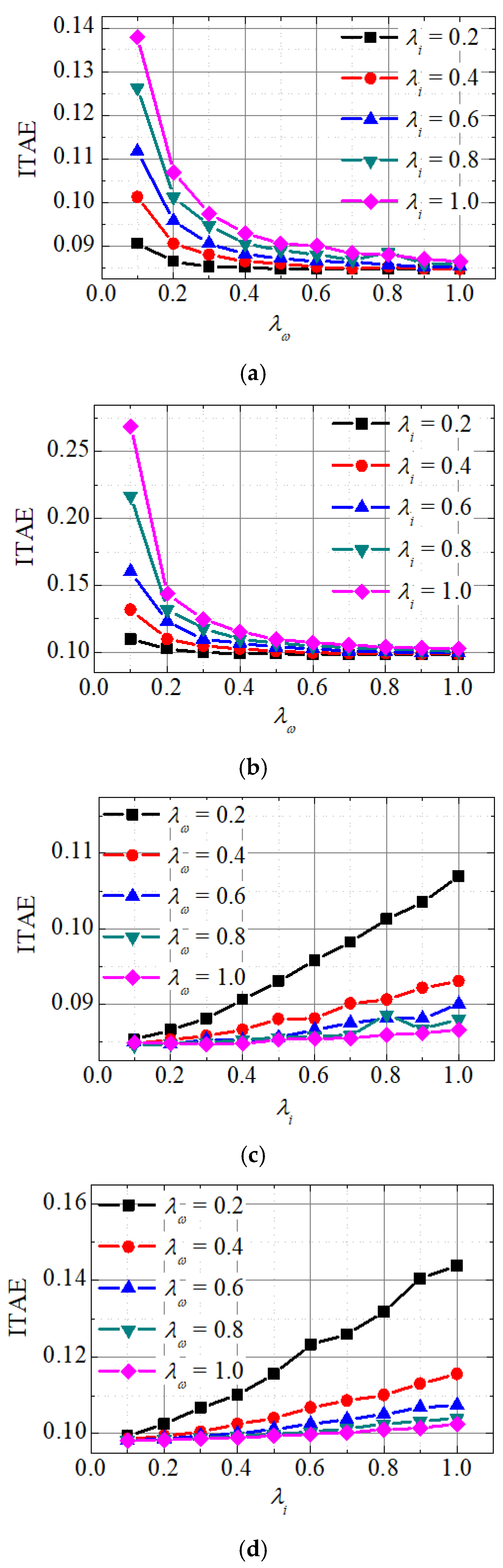
4.2. Weighting Factor Sensitivities

Weighting factors are inserted into the cost function when the control strategy includes several control targets, variables or constraints. The branch and bound algorithm is a frequently used weighting factor tuning method based on lots of simulation and experimental results. To assure control performance with inaccurate weighting factors, the system should not be sensitive to the weighting factors and that is an important index to make the system operate in a suitable state.

There are two weighting factors in (14) and the relationships between ITAEs and different weighting factors are shown in Figure 8. ITAEs are decreasing with the increasing of λ_ω and decreasing of λ_i. The rotor position ITAE variations are 35.876% and 63.456% for the NMPSC with proposed method and the conventional NMPSC method respectively, and the average rotor position ITAE values are 0.0902 and 0.1112 respectively, the increment is about 18.885%. The smoother waves of the proposed strategy imply lower sensitivities of the weighting factors.

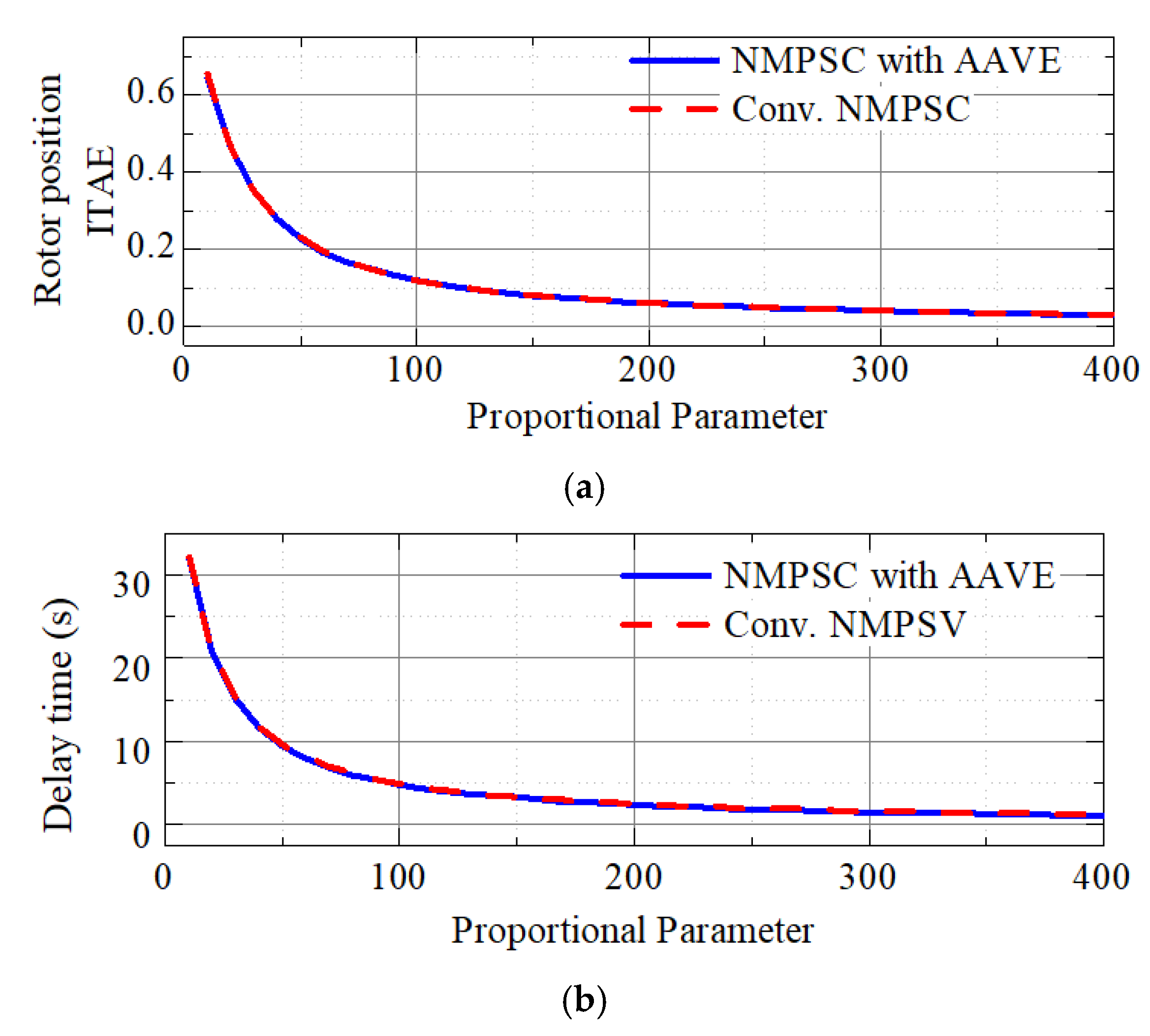
4.3. Propotional Parameter Selection

A proportional controller is adopted as the rotor position controller to resist overshoot and obtain better dynamics [31]. The waveforms for rotor position ITAEs and maximal delay time with different proportional parameters are shown in Figure 9, the rotor position ITAEs and maximal delay times have a similar tendency and the waveforms decrease with increasing of proportional coefficient values. As shown in the figures, when the proportional coefficient takes a value from 150 to 400 according to the branch and bound algorithm, the rotor ITAE and delay time are within appropriate ranges.

4.4. Proportional Parameter Selection

Some parameters including stator resistance R_s, stator induction L_s and magnet flux linkage ψ_m are always changing during operating states [4]. Defining R_se, L_se, and ψ_me as model parameters, different mismatches including R_se/R_s, L_se/L_s, and ψ_me/ψ_m are used to test stable operation ranges. The rotor position, error, and mismatch waves are shown in Figure 10. As shown in the figures, the stable ranges of parameter mismatches are 0.1~50, 0.1~1000 and 0.1~25 for R_se/R_s, L_se/L_s and ψ_me/ψ_m respectively.

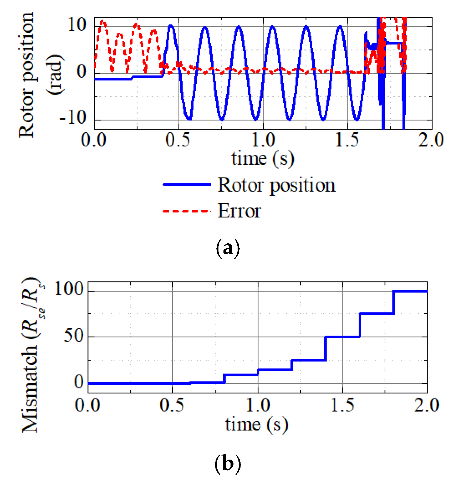
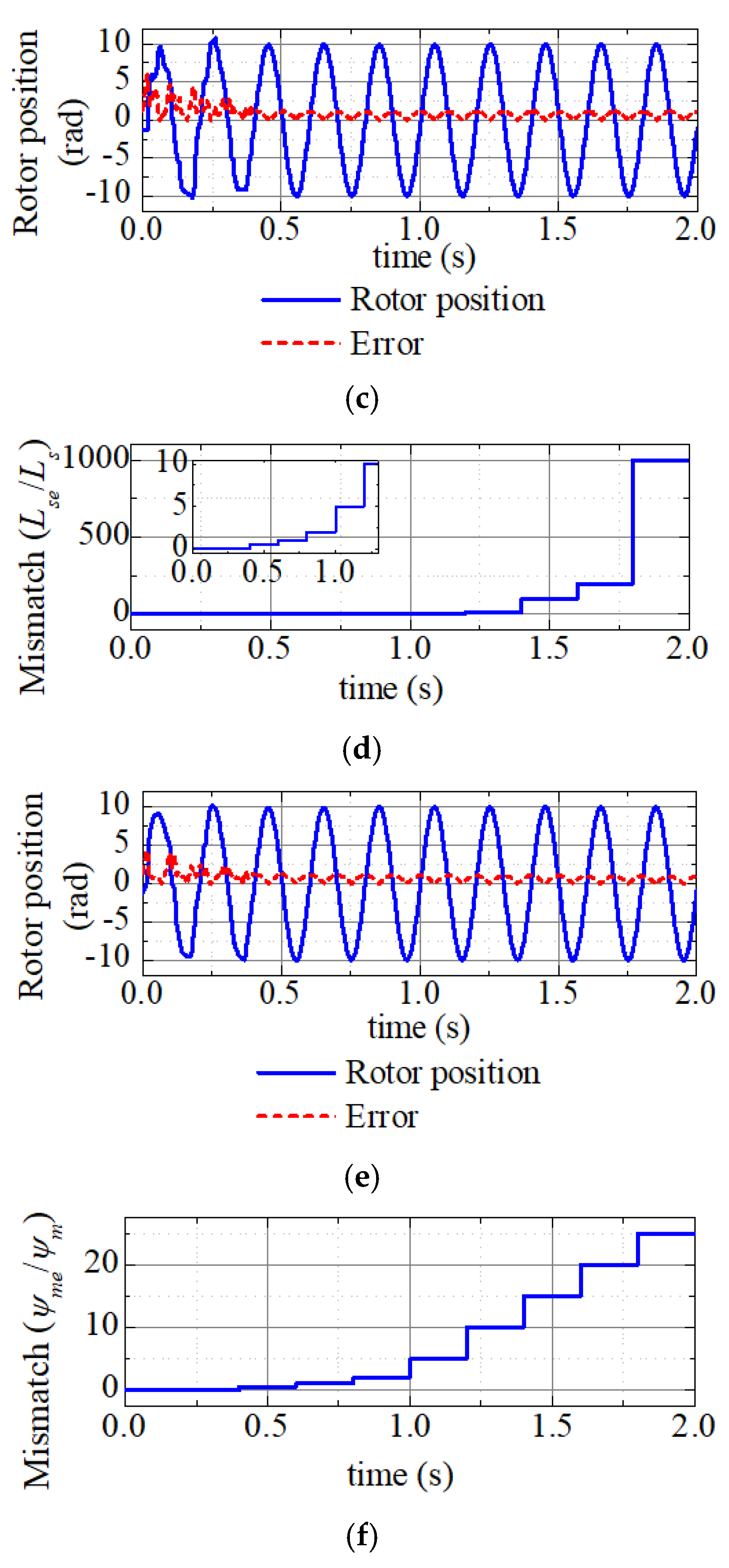
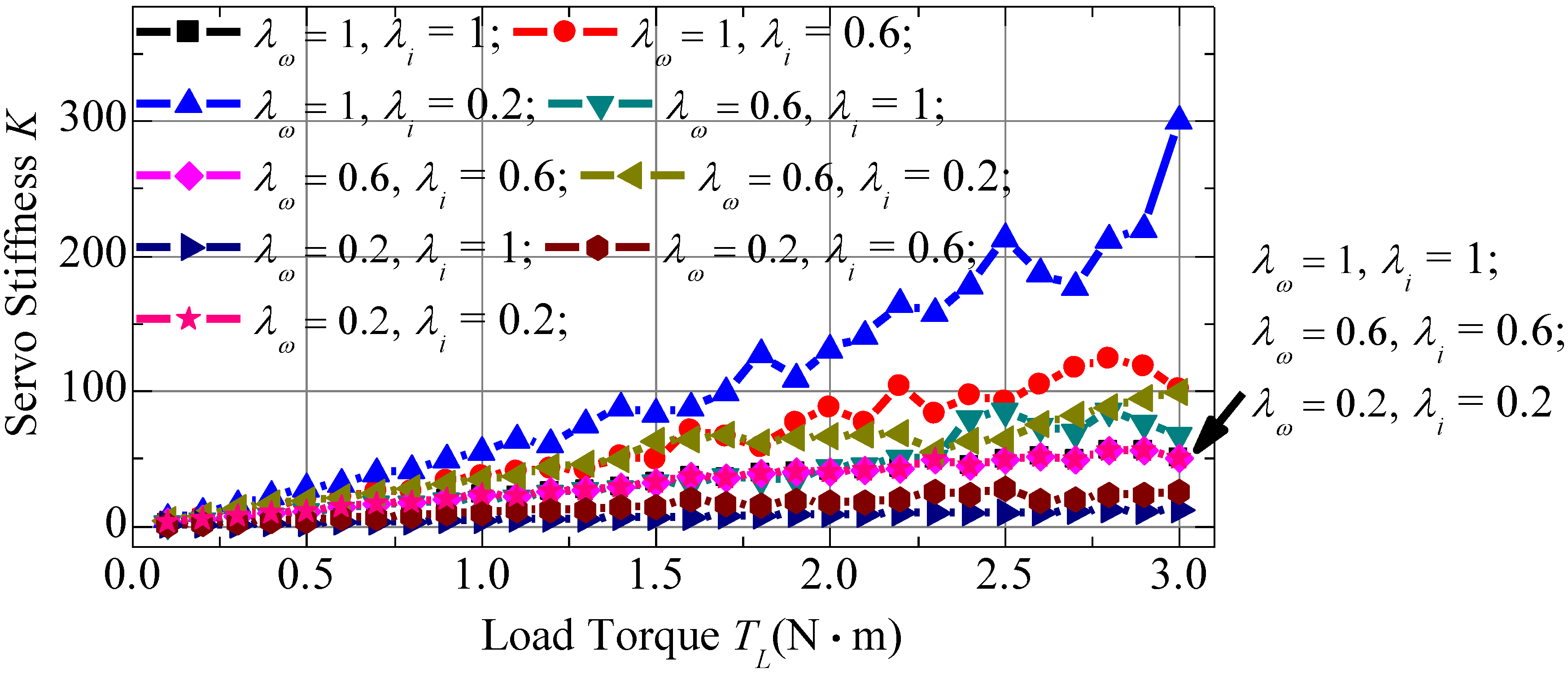
4.5. Servo Stiffness Analysis

Servo stiffness is an important index for the rotor position control system. This index reflects the rotor rotating angle generated by the load torque T_L which is uploaded on the shaft with a constant rotor reference. The definition is:

$$K=\left|\frac{T_L}{\mathsf{\Delta }\theta }\right|$$

(24)

The servo stiffness waveforms with different weighting factors are shown in Figure 11. The servo stiffness K increases as the load torque T_L increases. The one with λ_ω = 1 and λ_i = 0.2 has the highest servo stiffness, on the contrast, the one with λ_ω = 0.2 and λ_i = 1 has the lowest servo stiffness, which means that the former generates a less rotor angle change than the latter when a load torque is uploaded on the shaft with the same constant reference.

The average values and mean square error values of servo stiffness with different weighting factors for the proposed method and conventional method are listed in

Table 4. Comparison of servo stiffness with different weighting factors.

Control Strategies	Weighting Factors		Average Value of Servo Stiffness	Mean Square Error of Servo Stiffness
	λω	λi
NMPSC with the proposed method	1	1	31.6162	16.3266
	1	0.6	65.3566	52.0645
	1	0.2	105.8032	75.4438
	0.6	1	37.1100	26.0345
	0.6	0.6	31.6480	16.2684
	0.6	0.2	50.7884	26.2203
	0.2	1	6.5644	3.5587
	0.2	0.6	14.5511	7.8493
	0.2	0.2	31.6480	16.2684
Conventional NMPSC	1	1	18.3050	10.0392

. Under the same weighting factors, the average value and the mean square error value are larger in the proposed method than that in the conventional method.

Moreover, the ratio of the speed weighting factor λ_ω and the current weighting factor λ_i is also an important index for servo stiffness according to the waveforms and data. The same λ_ω/λ_i ratio will generate the same servo stiffness, for example, when λ_ω/λ_i = 1 (λ_ω = λ_i = 1, 0.6, 0.2), these three waveforms are the same as shown in Figure 11 and Table 4. The servo stiffness K increases as the ratio increases until the servo stiffness reaches the maximal value when the ratio equals 5, and vice versa.

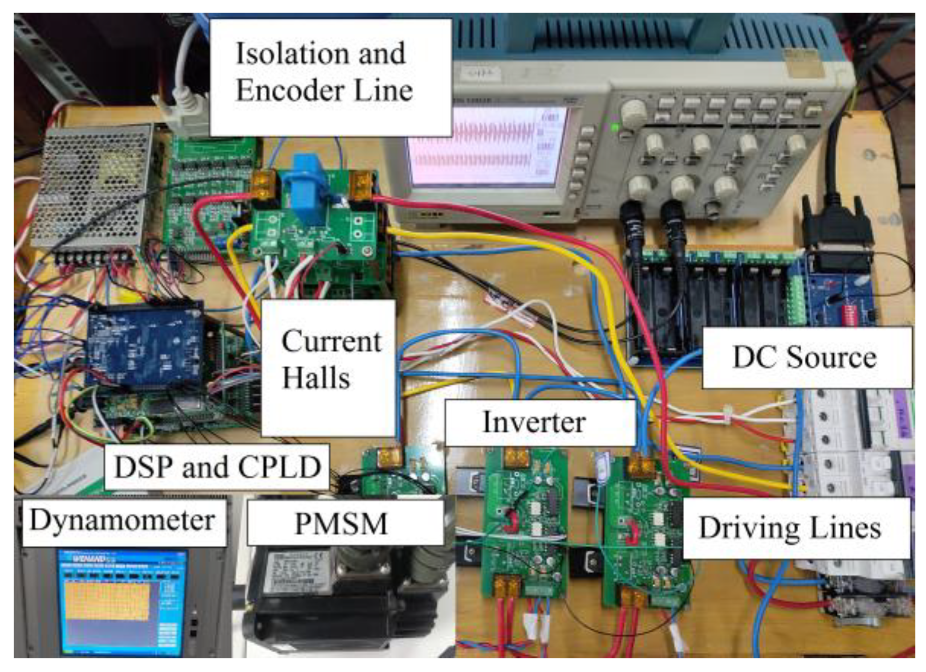
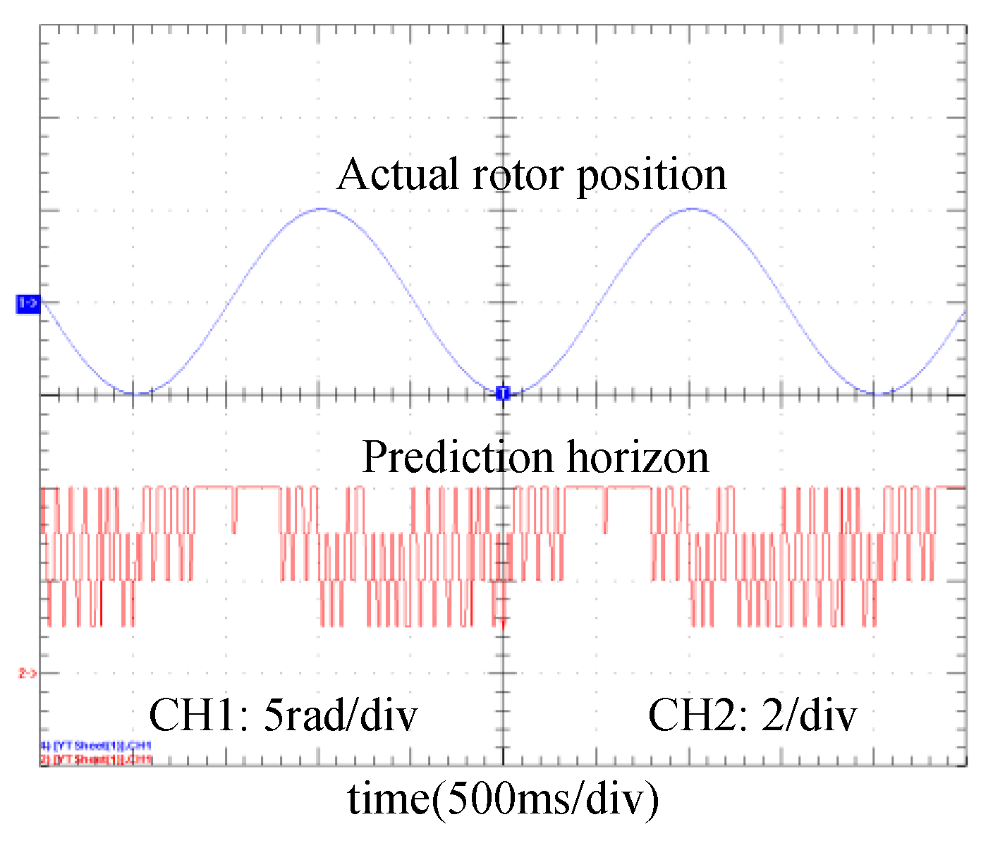
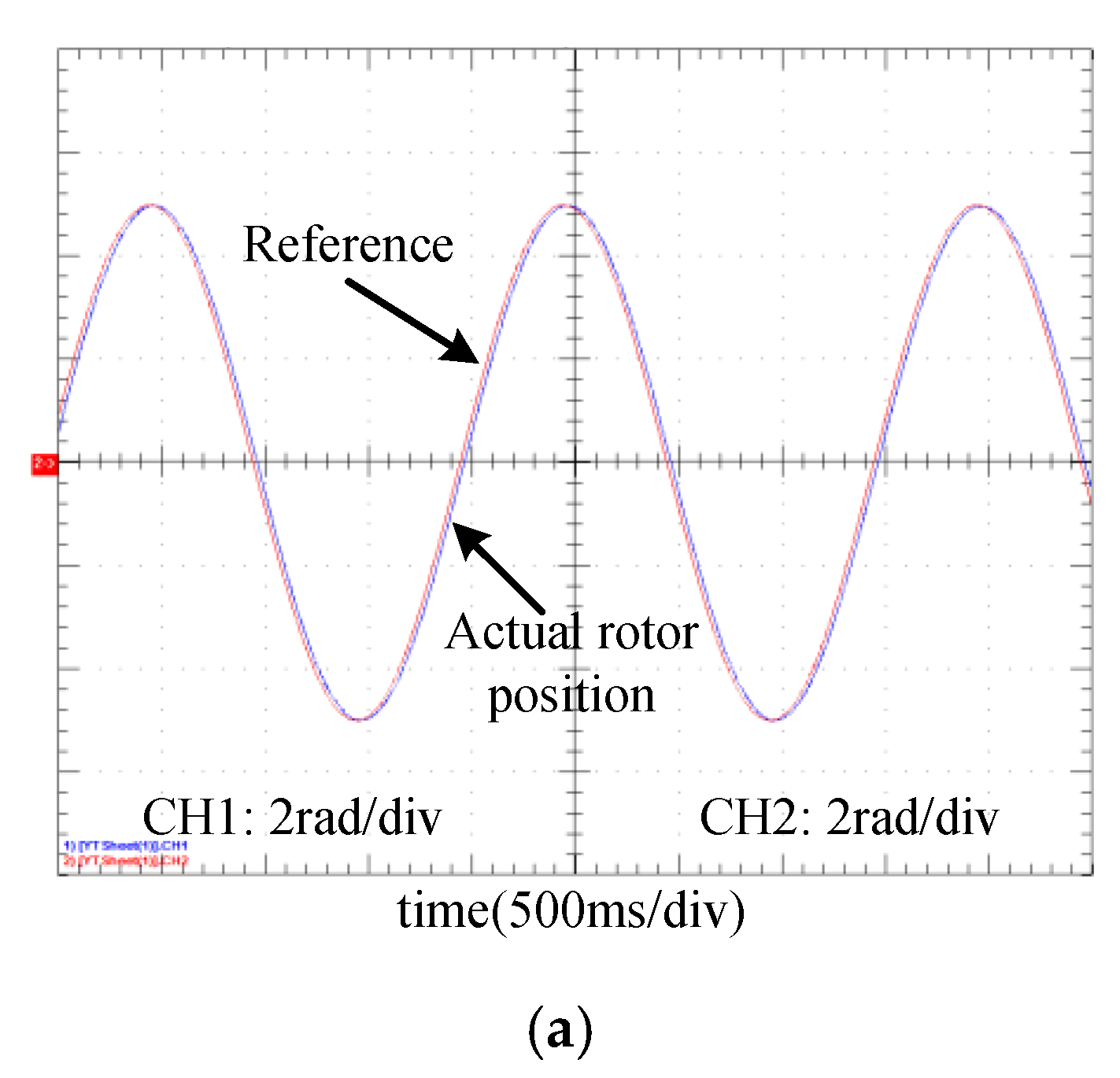
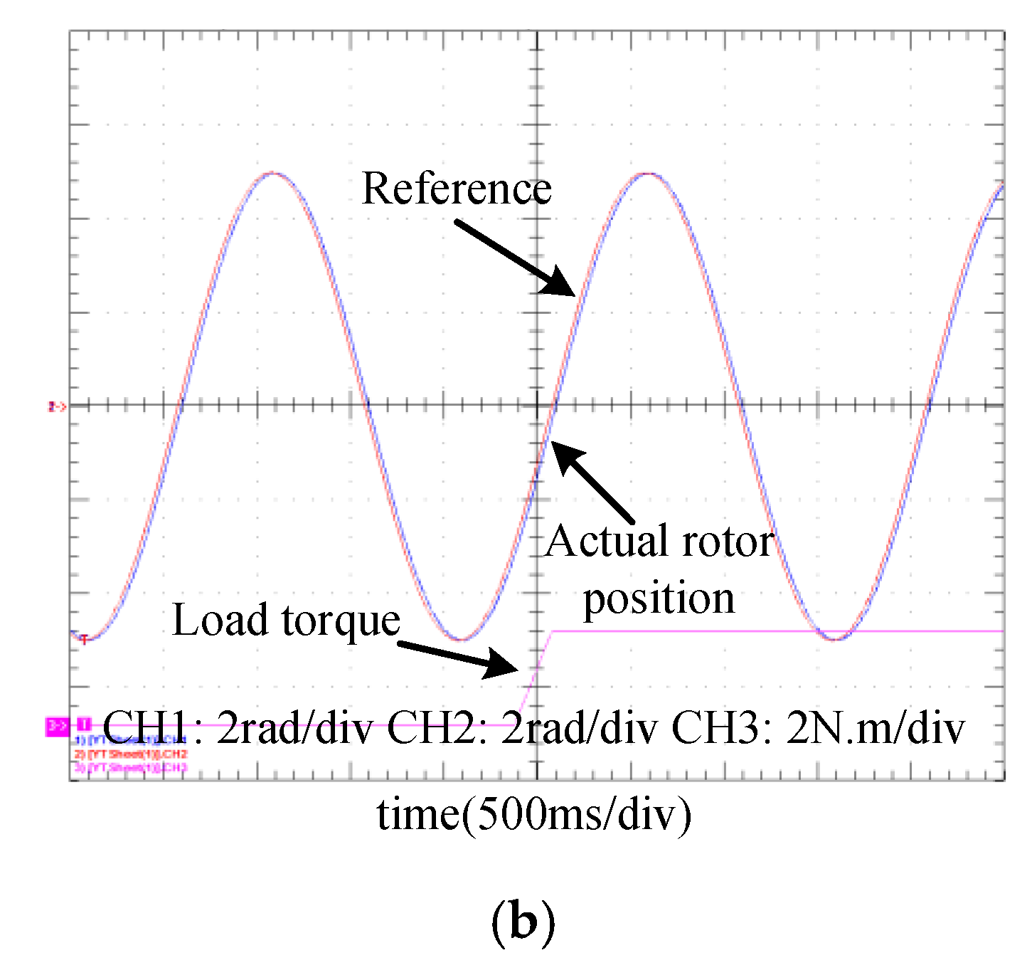
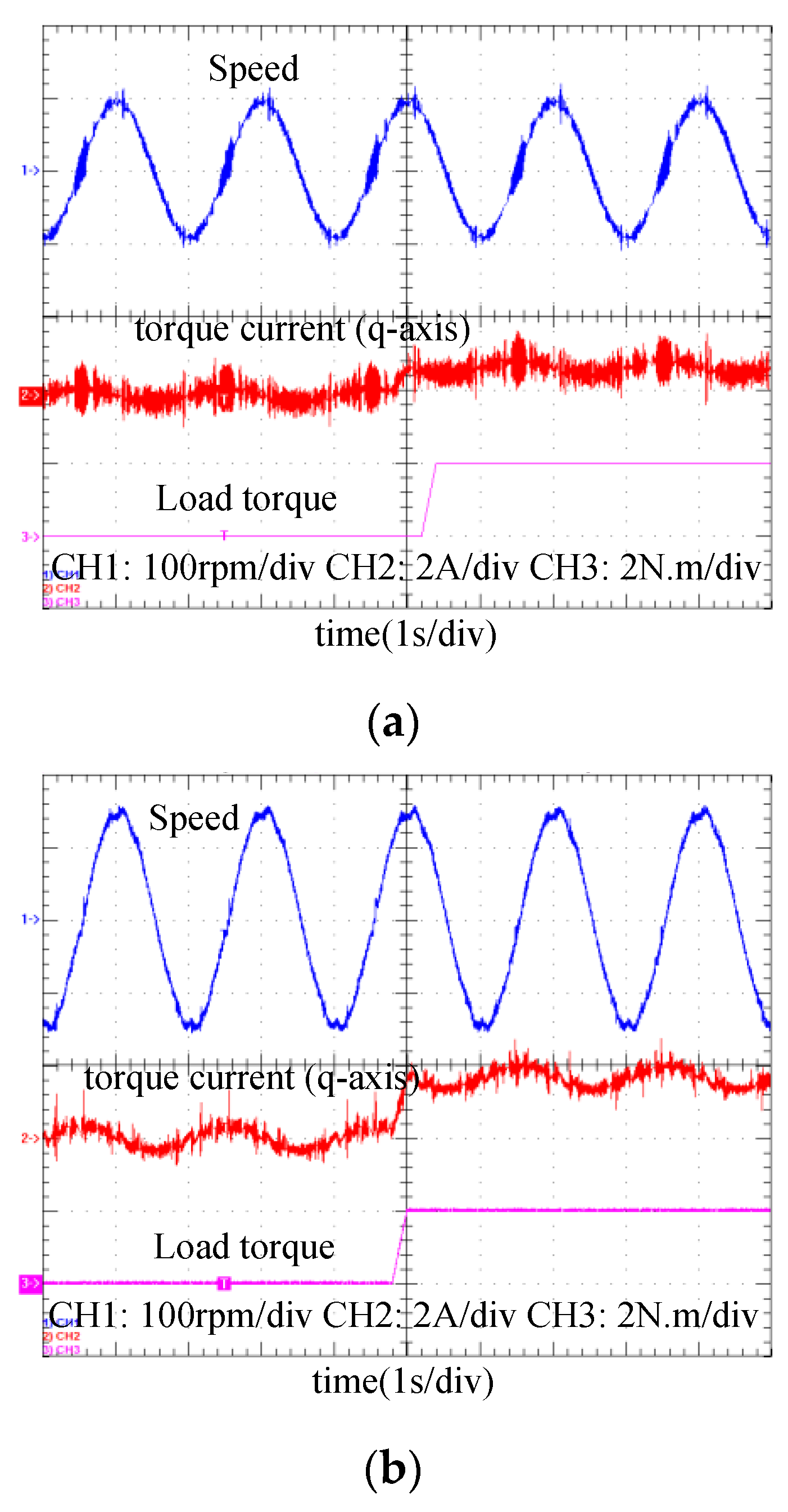
5. Experimental Results

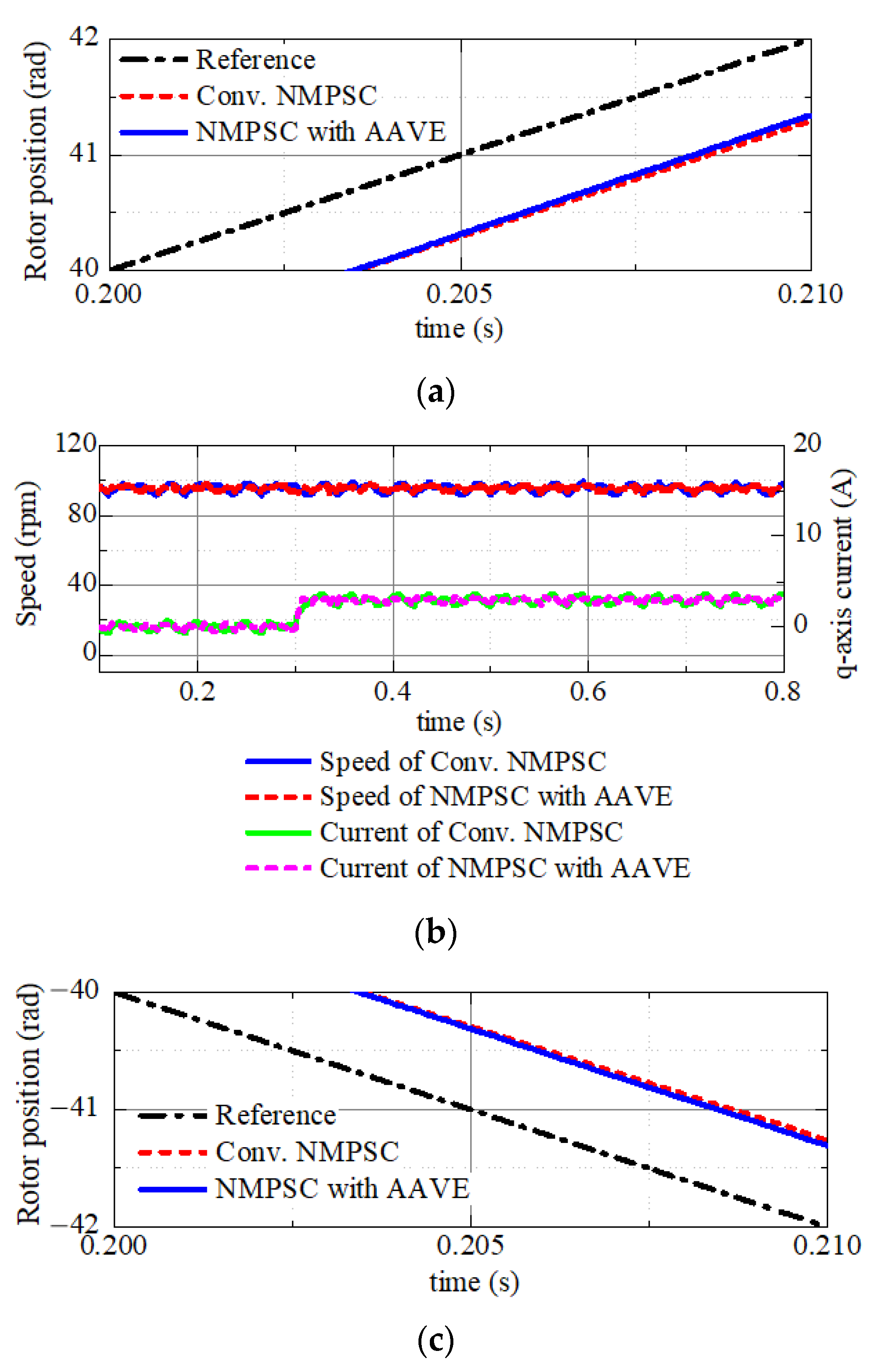
5.1. Tracking Comparison

The experimental setup is shown in Figure 12. A three-phase inverter with IGBTs (FGL35N120FTD) and a 1kW PMSM (INOVANCE ISMH2-10C30CD) with an incremental encoder (INOVANCE EI34H) are combined into the main circuit where the rated input voltage of the inverter is 800 V. The control strategy is accomplished by a DSP (TMS320F2812PGFA) and a CPLD (EPM240T100I-5N). The parameters of the PMSM in the experiment are the same as that of the simulation in Table 1, and the sampling period T_s is 0.1 ms. Importantly, the maximum prediction horizon N₂ is selected as 4 because of the calculation speed and the storage volume limitation of the hardware. λ_ω, λ_i, and the proportional parameters are 1, 0.5, and 300 respectively.

The prediction horizon waveform of the proposed method is shown in Figure 13, it is adjusted continuously rather than remaining unchanged value in the conventional strategy.

The rotor position and reference waveforms at steady-state and transient state are shown in Figure 14a,b respectively. It is shown that the actual rotor position can track the reference with a short delay time, and the disturbance can be resisted with little influence when a 2 N∙m load torque is uploaded onto the shaft.

Figure 15 provides the experimental results of conventional NMPSC strategy under the same conditions. It shows that longer delay time and larger static error are obtained than that in Figure 14, and a slight additional delay time, which is circled in the red dashed line shown in Figure 15b, is generated when the load torque uploads on the shaft.

Speed and filtered torque current (q-axis) waveforms for both strategies are shown in Figure 16a,b respectively. Both speed waves are operated in sinusoidal shape, and the amplitudes of speed and current waves are different. Since the rotor position can track the reference more closely by the proposed method, the speed continuously operates in a low-speed region comparing with the conventional NMPSC strategy, and the speed ripple is increased because detecting error cannot be eliminated on time due to the limited encoder accuracy, especially in the start and stop operating processes.

Some related experimental results of the NMPSC with the proposed method and the conventional NMPSC are listed in

Table 5. Performance comparison in three cycles.

Control Performances	NMPSC with the Proposed Method	Conventional NMPSC
Rotor position ITAE	2.323	2.734
Maximal speed	117.937 rpm	158.665 rpm
Maximal static error	0.366 rad	0.408 rad
Average prediction horizon	2.973	3 (Constant)
Maximal delay time	40 ms	52 ms

. The rotor position ITAE, maximal static error, and delay time within three cycles of the proposed method have been improved about 15.033%, 10.294%, and 23.077% respectively. Under the condition of the same proportional coefficient, obtained speed reference is lower than the conventional method, as a result, the maximum speed is less than the one achieved by the conventional method.

5.2. Computation Burden

In each sampling period, 8 vector candidates need to be evaluated in the cost function (14) of the proposed method. The circulate time of the conventional MPSC algorithm in [5] on the available experimental platform is about 25 μs, and it is about 65 μs for the conventional NMPSC algorithm above-mentioned in which the prediction horizon equals 3. For the NMPSC with a proposed method with 4 maximum prediction horizons, the maximal and average circulate time is about 85 μs and 64.415 μs, and the sampling interval is sufficient to execute without overruns. Due to the fact that the weighting factor optimization is performed offline, there is no additional computation burden during the execution of the algorithm [9], and the average circulates time of the proposed method is decreased about 0.9% compared with the conventional NMPSC strategy.

In a steady state, the calculation burden will be decreased because of the decreasing of the prediction horizon, and in a transient state, it is not increased even though the prediction horizon reaches 4 sometimes.

6. Conclusions

An NMPSC with AAVE prediction horizon self-tuning method with a discrete-time integral prediction horizon is proposed in this paper. The prediction horizon is adjusted online to the optimal value for different operating states. The PMSM angular velocity error is used to generate a virtual reference to adjust the prediction horizon for each sampling period. A comparative study is carried out between the proposed method and the conventional NMPSC with a constant prediction horizon. It shows that higher efficiency and servo stiffness, and lower weighting factor sensitivities, ITAEs, static errors, and delay times are obtained. Moreover, the experimental results show that high tracking performances are achieved for all operating processes, which are not demonstrated in an ideal simulation environment without delays of digital system.

Comparing with the conventional NMPSC, the rotor position ITAE of the NMPSC with the proposed method in three sinusoidal cycles is decreased about 15.033%, and the maximal static error and delay time is decreased about 10.294% and 23.077% respectively in experiments. Besides, the average value of calculation burden is decreased about 0.9% by adjustable prediction horizon, and the sensitivities of weighting factors and servo stiffness are improved about 18.885% and 42.102% respectively. The AAVE prediction horizon self-tuning method shows a better performance comparing with the conventional method.

Based on the proposed method, the future research work is to combine deterministic artificial intelligence (D.A.I.) with the prediction horizon tuning method to further improve the online tuning process and control performance, and the experimental realization of D.A.I. and MPC needs to be considered.

References

1. Tripathi, S.M.; Dutta, C. Enhanced efficiency in vector control of a Surface-mount PMSM drive. J. Frankl. Inst. 2018, 355, 2392–2423. [Google Scholar] [CrossRef]
2. Mondal, R.; Dey, J. Performance Analysis and Implementation of Fractional Order 2-DOF Control on Cart–Inverted Pendulum System. IEEE Trans. Ind. Appl. 2020, 56, 7055–7066. [Google Scholar] [CrossRef]
3. Li, P.; Zhu, G.; Zhang, M. Linear Active Disturbance Rejection Control for Servo Motor Systems with Input Delay via Internal Model Control Rules. IEEE Trans. Ind. Electron. 2021, 68, 1077–1086. [Google Scholar] [CrossRef]
4. Yan, L.; Wang, F.; Dou, M.; Zhang, Z.; Kennel, R.; Rodríguez, J. Active Disturbance-Rejection-Based Speed Control in Model Predictive Control for Induction Machines. IEEE Trans. Ind. Electron. 2020, 67, 2574–2692. [Google Scholar] [CrossRef]
5. Rodriguez, J.; Cortes, P. Predictive Control of Power Converters and Electrical Drives; IEEE Press-Wiley: Oxford, UK, 2012; pp. 133–176. [Google Scholar]
6. Wang, F.; Ke, D.; Yu, X.; Huang, D. Enhanced Predictive Model Based Deadbeat Control for PMSM Drives Using Exponential Extended State Observer. IEEE Trans. Ind. Electron. 2021. [Google Scholar] [CrossRef]
7. Wang, J.; Tang, Y.; Qi, Y.; Lin, P.; Zhang, Z. A Unified Startup Strategy for Modular Multilevel Converters with Deadbeat Predictive Current Control. IEEE Trans. Ind. Electron. 2021, 68, 6401–6411. [Google Scholar] [CrossRef]
8. Pei, G.; Li, L.; Gao, X.; Liu, J.; Kennel, R. Predictive Current Trajectory Control for PMSM at Voltage Limit. IEEE Access 2019, 8, 1670–1679. [Google Scholar] [CrossRef]
9. Novak, M.; Xie, H.; Dragicevic, T.; Wang, F.; Rodriguez, J.; Blaabjerg, F. Optimal Cost Function Parameter Design in Predictive Torque Control (PTC) Using Artificial Neural Networks (ANN). IEEE Trans. Ind. Electron. 2021, 68, 7309–7319. [Google Scholar] [CrossRef]
10. Wang, F.; Zuo, K.; Tao, P.; Rodriguez, J. High Performance Model Predictive Control for PMSM by using Stator Current Mathematical Model Self-Regulation Technique. IEEE Trans. Power Electron. 2020, 35, 13652–13662. [Google Scholar] [CrossRef]
11. Kawai, H.; Zhang, Z.; Kennel, R. Finite Control Set-Model Predictive Speed Control with a Voltage Smoother. In Proceedings of the 44th Annual Conference of the IEEE Industrial Electronics Society (IECON-2018), Washington, DC, USA, 21–23 October 2018. [Google Scholar]
12. Wang, F.; He, L. FPGA-Based Predictive Speed Control for PMSM System Using Integral Sliding-Mode Disturbance Observer. IEEE Trans. Ind. Electron. 2021, 68, 972–981. [Google Scholar] [CrossRef]
13. Wang, F. Control System Analysis and Design–Process Control System; Tsinghua University Press: Beijing, China, 2014; pp. 228–258. [Google Scholar]
14. Geyer, T. Model Predictive Control of High Power Converters and Industrial Drives; Wiley: London, UK, 2016; pp. 153–194. [Google Scholar]
15. Wei, Y.; Wei, Y.; Sun, Y.; Qi, H.; Guo, X. Prediction Horizons Optimized Nonlinear Predictive Control for PMSM Position System. IEEE Trans. Ind. Electron. 2020, 67, 9153–9163. [Google Scholar] [CrossRef]
16. Errouissi, R.; Ouhrouche, M. Nonlinear predictive controller for a permanent magnet synchronous motor drive. Math. Comput. Simul. 2010, 81, 394–406. [Google Scholar] [CrossRef]
17. Zhang, Y.; Yang, H. Two-Vector-based Model Predictive Torque Control without Weighting Factors for Induction Motor Drives. IEEE Trans. Power Electron. 2016, 31, 1381–1390. [Google Scholar] [CrossRef]
18. Wang, F.; Xie, H.; Chen, Q.; Davari, S.A.; Rodriguez, J.; Kennel, R. Parallel Predictive Torque Control for Induction Machines without Weighting Factors. IEEE Trans. Power Electron. 2020, 35, 1779–1788. [Google Scholar] [CrossRef]
19. Cortes, P.; Rodriguez, J.; Silva, C.; Flores, A. Delay Compensation in Model Predictive Current Control of a Three-Phase Inverter. IEEE Trans. Ind. Electron. 2012, 59, 1323–1325. [Google Scholar] [CrossRef]
20. Wang, X.; Sun, D. Three-Vector-Based Low-Complexity Model Predictive Direct Power Control Strategy for Doubly Fed Induction Generators. IEEE Trans. Power Electron. 2017, 32, 773–782. [Google Scholar] [CrossRef]
21. Wei, Y.; Li, M.; Wei, Y.; Qi, H. A Quadra-Layer Direct Speed SMPC Strategy for PMSM Rotor Position. In Proceedings of the 9th Frontier Academic Forum of Electrical Engineering (FAFEE 2020), Xi’an, China, 26–28 August 2020. [Google Scholar]
22. Kong, F.; Keyser, R.D. Criteria for choosing the horizon in extended horizon predictive control. IEEE Trans. Autom. Control 1994, 39, 1467–1470. [Google Scholar] [CrossRef]
23. Younesi, A.; Tohidi, S.; Feyzi, M.R.; Baradarannia, M. An improved nonlinear model predictive direct speed control of permanent magnet synchronous motors. Int. Trans. Elect. Energy Syst. 2018, 16, 2535–2550. [Google Scholar] [CrossRef]
24. Younesi, A.; Tohidi, S.; Feyzi, M.R. Improved Optimization Process for Nonlinear Model Predictive Control of PMSM. Iran. J. Elect. Electron. Eng. 2018, 14, 278–288. [Google Scholar]
25. Sun, Z.; Dai, L.; Liu, K.; Dimarogonas, D.V.; Xia, Y. Robust Self-Triggered MPC with Adaptive Prediction Horizon for Perturbed Nonlinear Systems. IEEE Trans. Autom. Control. 2019, 64, 4780–4787. [Google Scholar] [CrossRef]
26. Dong, L.; Yan, J.; Yuan, X.; He, H.; Sun, C. Functional Nonlinear Model Predictive Control Based on Adaptive Dynamic Programming. IEEE Trans. Cybern. 2019, 49, 4206–4218. [Google Scholar] [CrossRef] [PubMed]
27. Ionescu, C.M.; Copot, D.; Maxim, A.; Dulf, E.; Both, R.; Keyser, R.D. Robust Autotuning MPC for a Class of Process Control Applications. In Proceedings of the IEEE International Conference on Automation, Quality and Testing, Robotics (AQTR), Cluj-Napoca, Romania, 19–21 May 2016. [Google Scholar]
28. Bonilla, J.; Keyser, R.D.; Plaza, D. Nonlinear Predictive Control of a DC-DC Converter: A NEPSAC approach. In Proceedings of the 2007 European Control Conference (ECC), Kos, Greece, 2–5 July 2007. [Google Scholar]
29. Hernandez, A.; Keyser, R.D.; Dutta, A.; Nopens, I. Robust Nonlinear Extended Prediction Self-Adaptive Control (NEPSAC) of Continuous Bioreactors. In Proceedings of the Mediterranean Conference on Control & Automation (MED), Barcelona, Spain, 3–6 July 2012. [Google Scholar]
30. Chen, H. Stability and Robustness Considerations in Nonlinear Model Predictive Control; VDI: Verlag, Germany, 1997; pp. 153–194. [Google Scholar]
31. Kou, B.; Cheng, S. AC Servo Motor and Control Chap. 4; China Machine Press: Beijing, China, 2008; pp. 45–76. [Google Scholar]
Figure 1. Time flow of NMPC strategies. (a) Conventional NMPC; (b) Variable prediction horizon NMPC.
Electronics 10 01123 g001
Figure 2. Flowchart of NMPSC with the proposed VVAE method.
Electronics 10 01123 g002
Figure 3. Ideal functions u and v of the proposed AAVE method. (a) function v; (b) function u.
Electronics 10 01123 g003aElectronics 10 01123 g003b
Figure 4. Ideal functions ceil of the proposed AAVE method.
Electronics 10 01123 g004
Figure 5. Structure of PMSM rotor position system with the proposed method.
Electronics 10 01123 g005
Figure 6. Rotor position, error, and prediction horizon waveforms of the proposed NMPSC with AAVE method and the conventional NMPSC. (a) Rotor positions and errors; (b) Part enlarged rotor positions; (c) Part enlarged errors; (d) Prediction horizon.
Electronics 10 01123 g006
Figure 7. Simulation results of ramp references of the proposed NMPSC with AAVE method and conventional NMPSC. (a) Rotor positions with a positive slope; (b) Speed and torque current (q-axis) with a positive slope; (c) Rotor position with a negative slope; (d) Speed and torque current (q-axis) with a negative slope.
Electronics 10 01123 g007aElectronics 10 01123 g007b
Figure 8. Contour maps of rotor position ITAEs with different weighting factors for the conventional NMPSC and the NMPSC with the proposed method. (a) λω to ITAE for the NMPSC with AAVE method; (b) λω to ITAE for the conventional NMPSC; (c) λi to ITAE for the NMPSC with AAVE method; (d) λi to ITAE for the conventional NMPSC.
Electronics 10 01123 g008
Figure 9. Performances for different proportional parameter values. (a) Rotor position ITAE; (b) Delay time.
Electronics 10 01123 g009
Figure 10. Parameter mismatches for the proposed method. (a) Rotor position and error with Rse; (b) different mismatch degrees for Rse; (c) Rotor position and error with Lse; (d) Different mismatch degrees for Lse; (e) Rotor position and error with ψme; (f) Different mismatch degrees for ψme.
Electronics 10 01123 g010aElectronics 10 01123 g010b
Figure 11. Servo stiffness with different weighting factors for the proposed method.
Electronics 10 01123 g011
Figure 12. Experimental setup.
Electronics 10 01123 g012
Figure 13. Rotor position and prediction horizon experimental results of the NMPSC with the proposed method.
Electronics 10 01123 g013
Figure 14. Rotor position and reference experimental results of the NMPSC with the proposed method. (a) Steady-state; (b) Transient state.
Electronics 10 01123 g014aElectronics 10 01123 g014b
Figure 15. Rotor position and reference experimental results of the conventional NMPSC. (a) Steady-state; (b) Transient state.
Electronics 10 01123 g015
Figure 16. Speed and torque current (q-axis) experimental results. (a) NMPSC with the proposed method; (b) Conventional NMPSC.
Electronics 10 01123 g016