Deflated Restarting of Exponential Integrator Method with an Implicit Regularization for Efficient Transient Circuit Simulation

Abstract

Exponential integrator (EI) method based on Krylov subspace approximation is a promising method for large-scale transient circuit simulation. However, it suffers from the singularity problem and consumes large subspace dimensions for stiff circuits when using the ordinary Krylov subspace. Restarting schemes are commonly applied to reduce the subspace dimension, but they also slow down the convergence and degrade the overall computational efficiency. In this paper, we first devise an implicit and sparsity-preserving regularization technique to tackle the singularity problem facing EI in the ordinary Krylov subspace framework. Next, we analyze the root cause of the slow convergence of the ordinary Krylov subspace methods when applied to stiff circuits. Based on the analysis, we propose a deflated restarting scheme, compatible with the above regularization technique, to accelerate the convergence of restarted Krylov subspace approximation for EI methods. Numerical experiments demonstrate the effectiveness of the proposed regularization technique, and up to $50\%$ convergence improvements for Krylov subspace approximation compared to the non-deflated version.

1. Introduction

High performance and full-accuracy transient circuit simulation has always been one of the major demands in modern IC design industry. And its importance is increasing due to the fast-growing design complexities with advanced technology nodes. Besides IC design, SPICE-type simulators have also been widely used in some other scientific domains, such as electric/thermal analysis [1], electric/magnetic analysis [2], and advection-diffusion analysis [3], where the systems of interest can be described by differential algebraic equations (DAEs).

The essence of transient circuit simulation is to numerically solve a system of DAEs, normally derived from Modified Nodal Analysis (MNA), by an explicit or implicit integration method. Being a category of implicit methods, Backward differentiation formula (BDF) is widely adopted by existing SPICE simulators as it offers larger time steps and better stability than explicit methods. It is also more suitable for handling stiff DAEs with time constants differing by several orders of magnitude.

However, BDF is seeing elevated challenges in scalability, parallelizability and adaptivity as problem sizes grow into million-scale, or even billion-scale. The accuracy order of BDF is typically no higher than 2, which limits the step sizes and demands a large number of time steps. Often, it requires in each time step a sparse LU decomposition, which is known to be less scalable and parallelizable. Although considerable efforts have been dedicated to accelerating BDF-based transient simulation, new integration methods different from BDF might be needed to address the simulation capacity demands from the scientific and industrial communities.

Exponential integrator (EI) method is one of the emerging simulation methodologies to solve ordinary differential equations (ODEs) in a semi-analytical way, where the time span is discretized but the equation is solved analytically in each time step by expressing the solution in a matrix exponential form. For linear circuits, EI is in principle immune to the local truncation error (LTE) of polynomial expansion approximation in BDF [1,2,4,5,6,7]. The error only exists in the Krylov subspace approximation of the matrix exponential vector product; therefore, the accuracy order can be much higher than 2 without compromising stability [7]. Besides, only sparse matrix-vector multiplications are needed in EI method if the ordinary Krylov subspace is applied, which are highly scalable and parallelizable [8,9,10,11]. These advantages make EI a promising alternative to BDF for large-scale transient circuit simulation.

However, Krylov-subspace-based EI also has its own difficulties. One important issue is the singularity problem caused by the singular dynamic matrix of the DAE, which prohibits a straightforward conversion of the circuit DAE to an ODE required by EI. The singularity is mainly due to the algebraic constraints that do not involve time derivatives in the circuit, which leaves empty rows in the dynamic matrix. To solve the singularity problem, Chen has proposed a two-step DAE-ODE transformation for circuit simulation [5]. First, a topology-based approach is applied to reduce the DAE index of the circuit from 2 to 1, which can be skipped if the circuit is already index-1. Second, row echelon reduction is used to swap particular rows between the dynamic matrix and static matrix to eliminate the singularity. The problem lies in that the row echelon reduction is computationally expensive and tends to degrade the sparsity of the resulting matrices. Reference [4] proposed an implicit and sparsity-preserving regularization technique for EI, which is for the rational Krylov subspace only.

Another bottleneck lies in the large Krylov subspace that is needed for EI to handle stiff circuits, if the ordinary Krylov subspace is adopted. To maintain sufficient accuracy, the Krylov subspace dimension easily reaches several hundreds for intermediate stiffness. Storing a number of dense basis vectors in memory and performing full orthogonalization w.r.t. these vectors constitute substantial computational and memory challenges. One solution to this challenge is to use other types of Krylov subspace, such as the rational [8] or the extended Krylov subspace [12], which typically demands a much smaller subspace dimension. The cost, however, is extra LU factorizations that to some extent reduces the benefits of using EI. Another route, as motivated by the Krylov-subspace iterative solvers for linear systems, is to resort to restarting. Weng proposed a restarted scheme for EI [6], in which the Krylov subspace basis generation is restarted every m steps; thus, the memory footprint and orthogonalization cost is limited to a m-dimensional subspace. The drawback of such a simple restarting is that the convergence is slowed down. The total number of subspace dimension of restarted EI is higher than that of the non-restarted version, resulting in degraded performance.

In this paper, we aim to address the above two issues limiting the performance of EI for large stiff circuit simulation. We restrict our focus to linear circuit simulation in this work, though extension to nonlinear circuits is possible. Specifically, our main contributions are two-fold:

• We devise an implicit and algebraic regularization for EI based on the ordinary Krylov subspace, as it works directly on the original sparse matrices in an implicit manner without the row echelon reduction. This way the sparsity of the system matrices is preserved and the computational efficiency is improved.
• We propose a deflated restarting scheme for EI with the ordinary Krylov subspace. The scheme extracts some useful information from the previous round of Arnoldi process and incorporates such information into the new round of process, so as to accelerate the convergence of the Krylov subspace approximation. In other words, the proposed method “deflates” a subspace from the search space, so that the new search space is narrowed down and the convergence becomes faster compared to the non-deflated version. Some preliminary results have been reported in Reference [13], but an in-depth analysis of the root cause of the slow convergence and the optimal selection of the eigenvalues to be deflated are still missing.

With the two techniques, we aim to make EI comparable in robustness and superior in performance compared to BDF, rendering EI a practical alternative for future large-scale transient circuit simulation.

The paper is organized as follows. Section 2 introduces the EI formulation for transient circuit simulation. Section 3 presents the proposed regularization to tackle the singularity problem. Section 4 reveals the causes of the convergence problem of EI methods and proposes a deflated restarting scheme which is compatible with the above regularization to accelerate the convergence. Section 5 shows the numerical results, and Section 6 concludes the paper.

2. Background

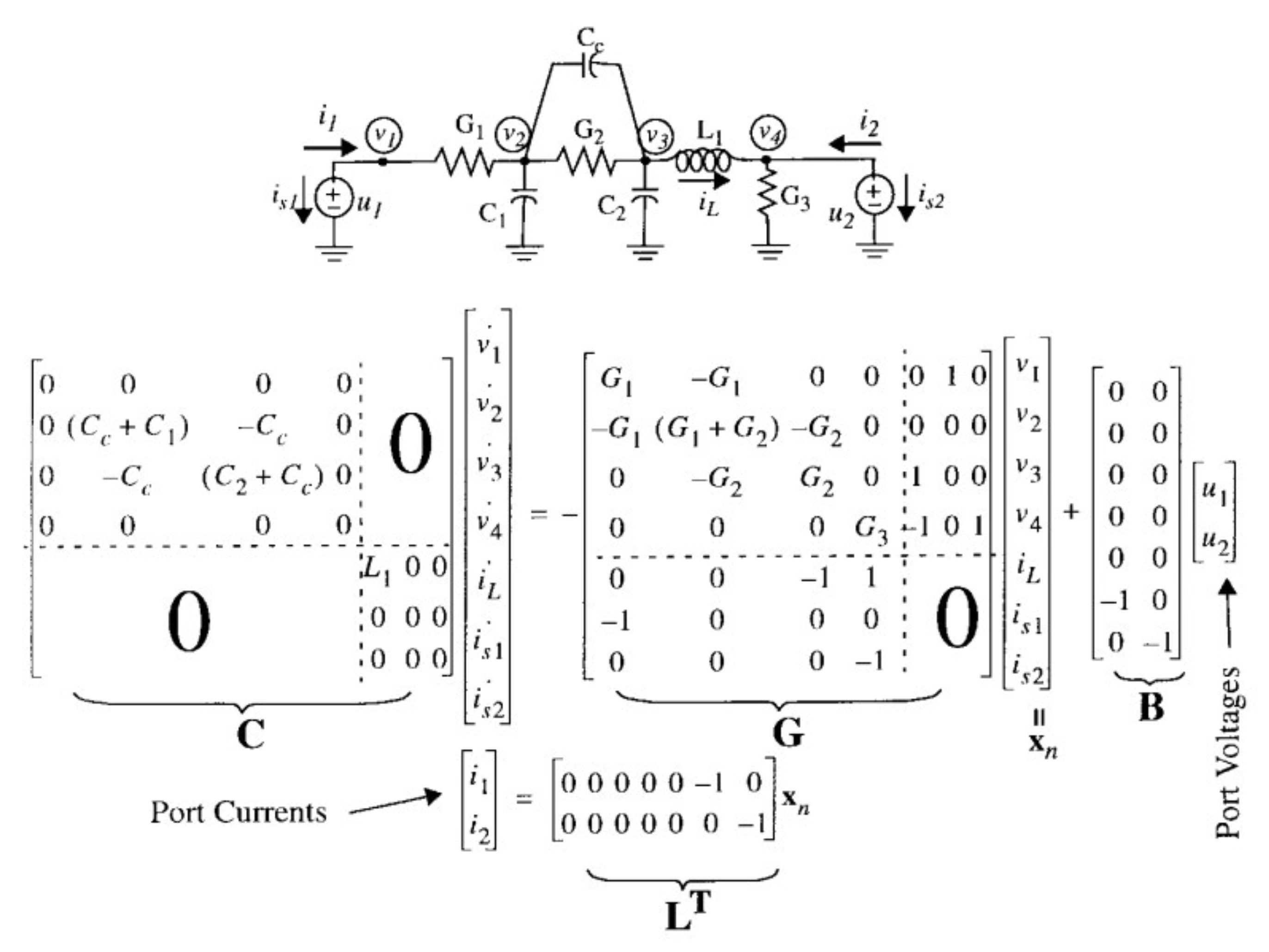
In transient circuit simulation, a linear circuit is described by the following DAE:

$$C\dot{x}\left(t\right)+Gx\left(t\right)=Bu\left(t\right),$$

(1)

where C and G represent the capacitance/inductance matrix and resistance/conductance matrix, respectively, and the matrix B indicates the locations of independent sources. $u\left(t\right)$ denotes the input source term. $x\left(t\right)$ is comprised of the unknown voltages and branch currents at time t. Figure 1 shows an example of (1).

We assume C is non-singular, the above DAE (1) can be directly transformed into an ODE:

$$\dot{x}\left(t\right)=Ax\left(t\right)+b\left(t\right),$$

(2)

where $A=-C^{-1}G$, $b\left(t\right)=C^{-1}Bu\left(t\right)$.

Then, the analytical solution for $x_{n+1}$ of the above ODE (2) can be solved with matrix exponential:

$$x_{n+1}=e^{Ah}{x}_n+\underset{0}{\overset{h}{\int }}{e}^{A(h-\tau )}b(t+\tau )d\tau ,$$

(3)

where h is the time step size.

The integral term in (3) can be computed analytically by applying the second-order piece-wise-linear (PWL) approximation $b(t+\tau )=b\left(t\right)+\frac{b(t+h)-b\left(t\right)}{h}\tau$ [14], which turns the solution into the sum of three matrix exponential functions.

$$x_{n+1}=e^{Ah}{x}_n+h{\phi }_1\left(Ah\right){\omega }_1+h^2{\phi }_2\left(Ah\right){\omega }_2,$$

(4)

where ${\omega }_1=C^{-1}Bu\left(t\right)$, ${\omega }_2=C^{-1}B(\frac{u(t+h)-u\left(t\right)}{h})$. And ${\omega }_2$ approximates the slope of input waveform.

The analytical solution (4) has three matrix exponential functions, which are generally referred as $\phi$ functions of the zero, first and second order.

$${\phi }_0\left(x\right)=e^x,{\phi }_1\left(x\right)=\frac{e^x-1}{x},{\phi }_2\left(x\right)=\frac{e^x-x-1}{x^2}.$$

Almohy [15] has shown that a series of $\phi$ functions can be calculated by computing the exponential of a $(n+p)\times (n+p)$ matrix, where n and p describe the dimension of A and the order of $\phi$ functions, respectively, which prevents from explicitly calculating each $\phi$ function. Therefore, we can merge the sum of the three terms of $\phi$ functions (4) into the exponential of an augmented matrix.

$${\tilde{x}}_{n+1}=\exp \left(\left[\begin{array}{cc}A& W\\ 0& J_2\end{array}\right]h\right)\left[\begin{array}{c}{x}_n\\ e_2\end{array}\right]=exp\left(\tilde{A}h\right){\tilde{x}}_n,$$

(5)

where

$$W=\left[\begin{array}{cc}{w}_2& w_1\end{array}\right],J_2=\left[\begin{array}{cc}0& 1\\ 0& 0\end{array}\right],e_2=\left[\begin{array}{c}0\\ 1\end{array}\right].$$

Due to the large matrix size (on the order of millions), direct computation of matrix exponential is prohibitive. However, the Krylov subspace approximation can be applied to reduce the problem to the evaluation of a much smaller matrix exponential by projecting the matrix exponential vector product (MEVP) in (5) onto a smaller Krylov subspace ${\mathcal{K}}_m(A,v)=span(v,Av,A^{2}v,\dots ,A^{m-1}v)$ with $m\ll n$ [16].

It computes an orthogonal basis $V_m$ of ${\mathcal{K}}_m(A,v)$ from the Arnoldi process; see Algorithm 1:

$$A{V}_m=V_m{H}_m+h_{m+1,m}{v}_{m+1}{e}_m^T,$$

(6)

where $H_m$ is the upper Hessenberg matrix, and $e_m$ is the mth column of identity matrix $I_m$.

Then, we project A onto the Krylov subspace and use (6) to derive an approximation of $e^{Ah}v$:

$$e^{Ah}v\approx V_m{V_m}^T{e}^{Ah}v=∥v∥V_m{e}^{H_{m}h}{e}_1,$$

(7)

where $e^{H_{m}h}$ can be conveniently evaluated by a dense matrix approach, and Saad [16] proposed a posteriori residue estimate applied to evaluate the approximation (7) quality.

$$res=∥v∥h_{m+1,m}C{v}_{m+1}{e}_m^T{\phi }_1\left(H_m\right)e_1.$$

(8)

Algorithm 1: Arnoldi Process

3. Implicit Regularization

Note that, in (2), we assume C is non-singular and transform the DAE (1) into the ODE (2) directly. However, C is generally singular, since the algebraic constraints without time derivatives result in empty rows or columns in C, which prevents the straightforward multiplication of $C^{-1}$ on both sides of the DAE (1). Higher-order singularity is also possible due to irregular circuit topologies [17].

To eliminate the singularity, Reference [5] has proposed a two-step topology-based regularization. The first step is to reduce the circuit to index-1 by breaking all C-V loops and L-I cutsets [18] in the circuit. The second step is to apply the row echelon reduction to eliminate the variables corresponding to the singular part of the system. However, such row echelon reduction is computationally expensive and does not preserve the sparsity of C and G (1). To enhance the efficiency of regularization for large-scale systems, in this section, we devise a new regularization technique, which is implicit, algebraic, and sparsity preserving. The regularization is applied to EI based on the ordinary Krylov subspace.

3.1. Partition

We firstly define semi-explicit DAEs as follows.

Definition 1.

A semi-explicit DAEs of index-1 admits the following partition and conditions [19]

$$\left[\begin{array}{cc}{C}_s& \\ & \end{array}\right]\left[\begin{array}{c}{\dot{x}}_1\left(t\right)\\ {\dot{x}}_2\left(t\right)\end{array}\right]+\left[\begin{array}{cc}{G}_{11}& G_{12}\\ G_{21}& G_{22}\end{array}\right]\left[\begin{array}{c}{x}_1\left(t\right)\\ x_2\left(t\right)\end{array}\right]=\left[\begin{array}{c}{U}_1\left(t\right)\\ U_2\left(t\right)\end{array}\right],$$

(9)

with

1. 

a singular sparse matrix C,

2. 

a non-singular sub-matrix $C_s$,

3. 

non-singular sub-matrices $G_{22}$.

The above partition can be obtained by re-arranging the nonzero part of C in (1) to the upper left corner. If the above conditions do not hold, the DAE (9) is typically index-2 or index-1 with floating capacitors. In such case, the topology-based method in Reference [5] can be applied to break the C-V loops and/L-I cutsets and eliminate the floating capacitors, rendering a system in the form of (9).

3.2. Regularization

From (9), we have the following formula.

$$C_s{\dot{x}}_1\left(t\right)+G_{11}{x}_1\left(t\right)+G_{12}{x}_2\left(t\right)=U_1\left(t\right),$$

(10)

$$G_{21}{x}_1\left(t\right)+G_{22}{x}_2\left(t\right)=U_2\left(t\right).$$

(11)

Next, we can eliminate $x_2$ from (10) using (11), which yields

$$C_s{\dot{x}}_1\left(t\right)+(G_{11}-G_{12}{G}_{22}^{-1}{G}_{21})x_1\left(t\right)=U_1\left(t\right)-G_{12}{G}_{22}^{-1}{U}_2\left(t\right),$$

(12)

$$x_2\left(t\right)=G_{22}^{-1}(U_2\left(t\right)-G_{21}{x}_1\left(t\right)).$$

(13)

With (12), $x_1$ can be solved normally with the EI method, while $x_2$ is obtained by solving the algebraic Equation (13) after $x_1$ is solved. For simplicity, we denote

$$\begin{array}{cc}\hfill G_s& =G_{11}-G_{12}{G}_{22}^{-1}{G}_{21},\hfill \end{array}$$

(14)

$$\begin{array}{cc}\hfill b_s\left(t\right)& =U_1\left(t\right)-G_{12}{G}_{22}^{-1}{U}_2\left(t\right),\hfill \end{array}$$

(15)

and we obtain the ODE we need to solve (12) as:

$$C_s{\dot{x}}_1\left(t\right)+G_s{x}_1\left(t\right)=b_s\left(t\right).$$

(16)

Then, we multiply $C_s^{-1}$ on both sides of (16) and transform the above DAE to an ODE. And the ODE can be solved analytically by EI assuming PWL inputs:

$$x_{1,n+1}=x_{1,n}+h{\phi }_1\left(A_{s}h\right){\omega }_{s,1}+h^2{\phi }_2\left(A_{s}h\right){\omega }_{s,2},$$

(17)

where $A_s=-C_s^{-1}{G}_s$, ${\omega }_{s,1}=C_s^{-1}{b}_s\left(t\right)$, ${\omega }_{s,2}=C_s^{-1}\mathsf{\Delta }{b}_s\left(t\right).$

$$\begin{array}{cc}{e}^{{\tilde{A}}_{s}h}{\tilde{x}}_{1,n}\hfill & =exp\left(\left[\begin{array}{cc}-C_s^{-1}{G}_s& C_s^{-1}{W}_s\\ & J_2\end{array}\right]h\right)\left[\begin{array}{c}{x}_{1,n}\\ e_2\end{array}\right]\hfill \\ & =exp\left({\left[\begin{array}{cc}{C}_s/\alpha & \\ & I_2\end{array}\right]}^{-1}\left[\begin{array}{cc}-G_s& W_s\\ & \alpha J_2\end{array}\right]\frac{h}{\alpha }\right)\left[\begin{array}{c}{x}_{1,n}\\ e_2\end{array}\right]\hfill \\ & =exp\left(\left({\left[\begin{array}{cc}{C}_s/\alpha & \\ & I_2\end{array}\right]}^{-1}\left[\begin{array}{cc}-G_s-C_s/\alpha & W_s\\ & \alpha J_2-I_2\end{array}\right]+\left[\begin{array}{cc}{I}_s& \\ & I_2\end{array}\right]\right)\frac{h}{\alpha }\right)\left[\begin{array}{c}{x}_{1,n}\\ e_2\end{array}\right]\hfill \\ & =exp\left(\underset{{\widehat{C}}_s^{-1}}{\underbrace{{\left[\begin{array}{cc}{C}_s/\alpha & \\ & I_2\end{array}\right]}^{-1}}}\underset{{\widehat{G}}_s}{\underbrace{\left[\begin{array}{cc}-G_s-C_s/\alpha & W_s\\ & \alpha J_2-I_2\end{array}\right]}}\frac{h}{\alpha }\right)\underset{{\widehat{x}}_{1,n}}{\underbrace{\left[\begin{array}{c}{x}_{1,n}\\ e_2\end{array}\right]exp\left(\frac{h}{\alpha }\right)}}=e^{{\widehat{A}}_{s}h}{\widehat{x}}_{1,n}where{\widehat{A}}_s=\frac{1}{\alpha }{\widehat{C}}_s^{-1}{\widehat{G}}_s\hfill \end{array}.$$

(18)

Merging the three $\phi$ functions in (17) yields:

$$x_{1,n+1}=\left[\begin{array}{cc}{I}_n& 0\end{array}\right]exp\left({\tilde{A}}_{s}h\right){\tilde{x}}_{1,n},$$

(19)

where

$${\tilde{A}}_s=-{\left[\begin{array}{cc}{C}_s& \\ & I_2\end{array}\right]}^{-1}\left[\begin{array}{cc}{G}_s& -W_s\\ & -J_2\end{array}\right]=\left[\begin{array}{cc}-C_s^{-1}{G}_s& C_s^{-1}{W}_s\\ & J_2\end{array}\right]$$

$${\tilde{x}}_{1,n}=\left[\begin{array}{c}{x}_{1,n}\\ e_2\end{array}\right],C_s^{-1}{W}_s=\left[\begin{array}{cc}{\omega }_{s,2}& {\omega }_{s,1}\end{array}\right].$$

Each Arnoldi step requires the computation:

$${\tilde{A}}_s{\tilde{v}}_s=\left[\begin{array}{cc}-C_s^{-1}{G}_s& C_s^{-1}{W}_s\\ & J_2\end{array}\right]\left[\begin{array}{c}{v}_1\\ v_2\end{array}\right]=\left[\begin{array}{c}{C}_s^{-1}(-G_s+W_s)v_1\\ J_2{v}_2\end{array}\right]$$

(20)

The parameter $\alpha$ in (18) is a scaling factor introduced to balance the quantities in $C_s$ and $G_s$. Besides, the augmented matrix ${\tilde{A}}_s$ is transformed into a nonsingular matrix ${\widehat{A}}_s$ as derived in (18).

Then, the computation in each Arnoldi step requires solving:

$$\begin{array}{cc}{\widehat{A}}_s{\widehat{v}}_s\hfill & =\kappa {\left[\begin{array}{cc}{C}_s/\alpha & \\ & I_2\end{array}\right]}^{-1}\left[\begin{array}{cc}-G_s-C_s/\alpha & W_s\\ & \alpha J_2-I_2\end{array}\right]\left[\begin{array}{c}{v}_1\\ v_2\end{array}\right]\hfill \\ \hfill & =\kappa \left[\begin{array}{c}{(C_s/\alpha )}^{-1}\left[(-G_s-C_s/\alpha )v_1+W_s{v}_2\right]\\ (\alpha J_2-I_2)v_2\end{array}\right],\hfill \end{array}$$

(21)

where $\kappa$ is a scalar quantity, and $\kappa =\frac{h}{\alpha }exp\left(\frac{h}{\alpha }\right)$. Specifically, the core computation in Equation (21) is:

$$y_s={(C_s/\alpha )}^{-1}\left[(-G_s-C_s/\alpha )v_1+W_s{v}_2\right],$$

(22)

where

$$W_s=\left[b_{s,n},\mathsf{\Delta }{b}_s\right],\mathsf{\Delta }{b}_s=(b_{s,n+1}-b_{s,n})/h.$$

The main challenge in computing (22) lies in that the regularized matrices $G_s$ and $W_s$ in (22) are rather expensive to compute and tend to have much worse sparsity compared to the original matrices G and W, especially when $G_{22}$ is large. Hence, it is not recommended to explicitly form the matrices $G_s$ and $W_s$ for computing (22). Instead, we propose to compute $y_s$ in the following implicit and sparsity-preserving manner.

Firstly, we partition the original W matrix following the partition in (9).

$$W=\left[U\left(t\right),\mathsf{\Delta }U\left(t\right)\right]=\left[\begin{array}{cc}{U}_1\left(t\right)& \mathsf{\Delta }{U}_1\left(t\right)\\ U_2\left(t\right)& \mathsf{\Delta }{U}_2\left(t\right)\end{array}\right]=\left[\begin{array}{c}{W}_1\\ W_2\end{array}\right].$$

(23)

And we have $W_s=W_1-G_{12}{G}_{22}^{-1}{W}_2$.

Substituting the expressions of $G_s$ (14) and $W_s$ into (22) then yields:

$$\begin{array}{cc}{y}_s\hfill & ={(C_s/\alpha )}^{-1}[(-G_{11}+G_{12}{G}_{22}^{-1}{G}_{21}-C_s/\alpha )v_1+(W_1-G_{12}{G}_{22}^{-1}{W}_2)v_2]\hfill \\ \hfill & ={(C_s/\alpha )}^{-1}\underset{P_1}{\underbrace{[G_{12}{G}_{22}^{-1}(G_{21}{v}_1-W_2{v}_2)}}+\underset{P_2}{\underbrace{(-G_{11}-C_s/\alpha )v_1+W_1{v}_2]}}\hfill \end{array},$$

(24)

i.e., $y_s={(C_s/\alpha )}^{-1}\left(P_1+P_2\right)$. $P_2$ can be directly computed by matrix-vector multiplications with the corresponding blocks. $P_1$ can be solved by three steps:

• Compute $rh{s}_{1,2}=G_{21}{v}_1-W_2{v}_2$,
• Solve $x_{1,2}$ from $G_{22}{x}_{1,2}=rh{s}_{1,2}$,
• Compute $P_1=G_{12}{x}_{1,2}$.

The starting vector $v_s$ is obtained as follows:

$$v=\left[\begin{array}{c}{v}_s\\ v_p\end{array}\right]\Rightarrow v_s,$$

(25)

where $v_s$ has the same index as $C_s$. And to merge the three $\phi$ functions, we augment $v_s$ in (25) with $e_2$.

$${\tilde{v}}_s=\left[\begin{array}{c}{v}_s\\ e_2\end{array}\right]\Leftarrow e_2=\left[\begin{array}{c}0\\ 1\end{array}\right].$$

(26)

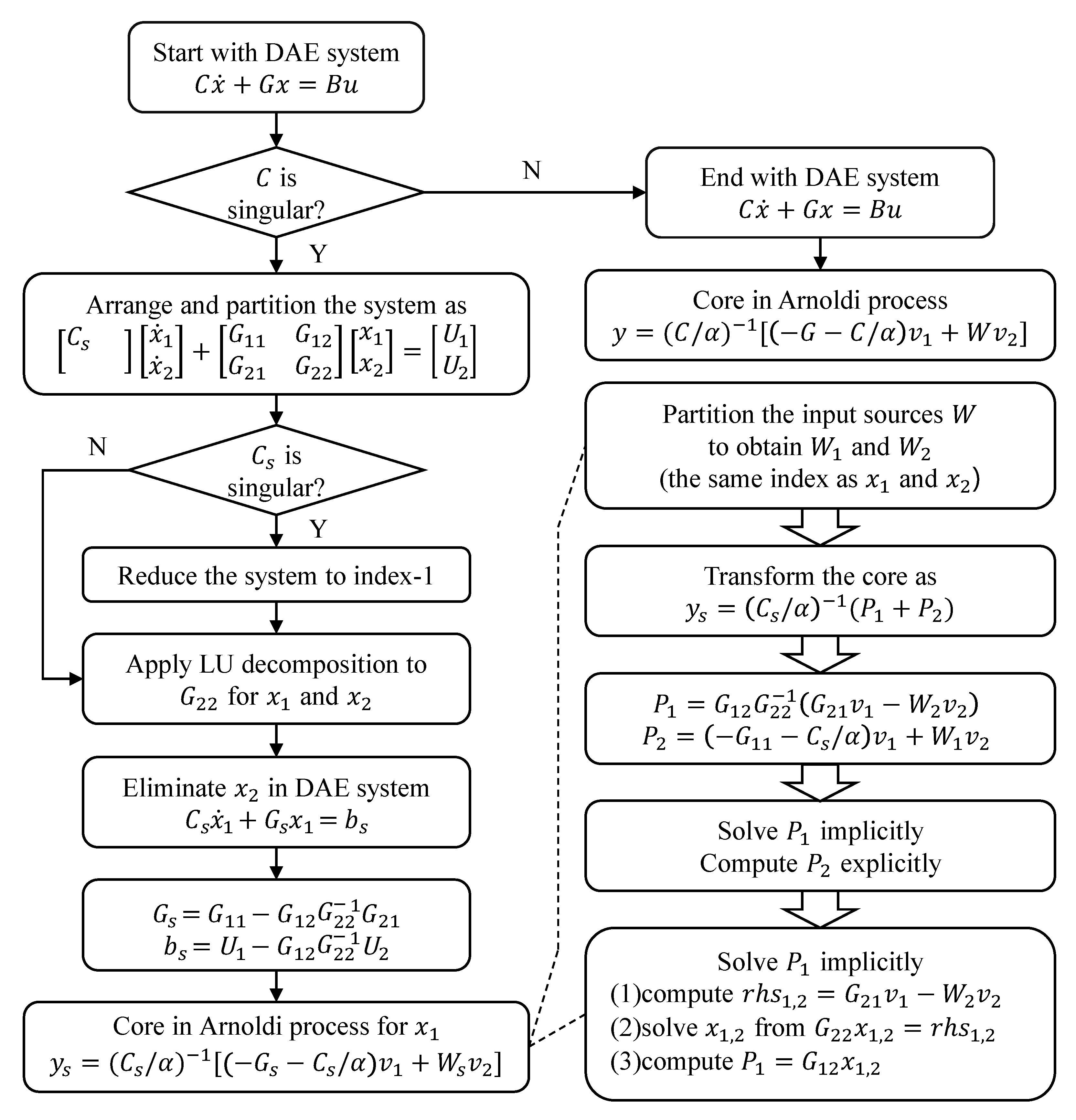
Given a solution v, we start the Arnoldi process with regularization. See Algorithm 2. Once we obtain one part of the solution in (12), the other part is solved algebraically in (13). The whole flow of our regularization is illustrated in Figure 2.

Two remarks are in order:

• The proposed regularization technique is “algebraic” in the sense that it works directly on the matrix level instead of the circuit topology level. It is “implicit” and “sparsity-preserving” since we do not explicitly form $G_s$ and $W_s$, but instead use the original sparse matrices C, G, W and their blocks in the computation.
• In Algorithm 2, each Arnoldi step involves two linear system solutions, one with $C_s$ and another with $G_{22}$. The former is needed for any variation of EI using the ordinary Krylov subspace approximation, while the latter is specifically associated to the proposed regularization technique. Since both the two sub-matrices are constant throughout the simulation, we only need to perform 1 sparse LU factorization for each matrix at the beginning, then re-use the LU factors in all subsequent computations. Thus, the overhead due to the proposed regularization is mild. In contrast, the rational Krylov subspace approach requires to factorize $C+G$, which is generally much more costly due to the enlarged size and a higher number of nonzeros.

Algorithm 2: Arnoldi Process with Regularization

4. Deflated Restarting of Exponential Integrator

Another challenge facing EI with ordinary Krylov subspace is the large subspace dimension required for stiff circuits. The stiffness appears when the time constants of the circuits differ by several orders of magnitudes. To guarantee the simulation accuracy of stiff circuits, one needs to either use small step sizes or a large Krylov subspace dimension m, with commonly $m>100$. For large problems, storing and performing orthogonalization with all the basis vectors can be highly memory and computation demanding. Moving big chunks of data back and forth between memory and CPU also induces large overheads and hampers parallelizability.

Therefore, there has been a strong desire to limit the subspace dimension for EI when handling stiff circuits. Motivated by the restarting scheme for Krylov subspace iterative solvers (such as GMRES), Reference [6] proposed a restarted Krylov subspace EI method in which the generation of Krylov subspace is restarted after a moderate number of Arnoldi steps, which reduces the memory and orthogonalization cost. However, simple restarting typically results in slower convergence compared to the no-restarted version, consuming more Arnoldi iterations and offsetting the benefit of restarting. In the next parts, we will first analyze the cause of the slow convergence of the ordinary Krylov subspace for stiff circuits, and then propose a deflated restarting scheme to accelerate the convergence by “deflating” certain subspace in the new search space. The deflated restarting scheme is also compatible with the implicit regularization technique described above.

4.1. Slow Convergence in Krylov Subspace Approximation for Stiff Circuits

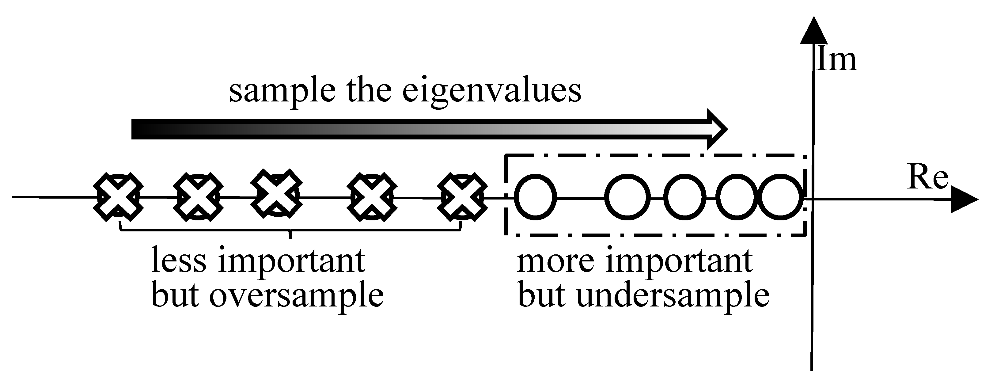
The dimension m required to accurately approximate $e^{A}v$ depends mainly on the eigenvalue distribution of the original projected matrix $A=-C^{-1}G$. The underlying idea is that the eigenvalues of $H_m$ in (6), or the Ritz values, gradually approximate the eigenvalues of A, and the basis $V_m$ gradually forms an orthogonal basis of the subspace spanned by the approximate eigenvectors of A. Being a variant of power iteration, the Arnoldi process is known to approximate large-magnitude (negative) eigenvalues with a higher priority [20]. More specifically, the Arnoldi process spends most of its “dimension resources” building a Krylov subspace spanned by the eigenvectors corresponding to those large-magnitude eigenvalues in A, while leaving fewer “resources” to the subspace corresponding to the small-magnitude eigenvalues. However, for transient circuit simulation, the approximation quality of small (magnitude) eigenvalues is more important than that of the larger ones in deciding the final accuracy. This can be explained by the fact that $e^{-\lambda }\approx 0$ when $\lambda \gg 1$, which means an accurate capture of large-magnitude eigenvalues is not necessary since their contributions to the solution are almost zero. On the other hand, small eigenvalues have more tangible impacts on the approximation accuracy.

Consequently, the key problem with the ordinary Krylov subspace EI (6) is that it oversamples the less important region but undersamples the more important region, in the matrix spectrum, as illustrated in Figure 3. For stiff circuits, the gap between small and large eigenvalues becomes more significant, thus demanding a larger subspace to ensure adequate sampling in the critical part of the spectrum.

4.2. Ordinary Restarted Krylov Subspace Method

To mitigate the large subspace dimension m required for stiff circuits, Reference [6] proposed a restarted Krylov subspace method specific for EI [21]. The Arnoldi process is restarted every m iterations, with the last basis vector $v_{m+1}$ in (6) in the current run being the initial vector $v_1$ of the next m-step Arnoldi process.

$$A{V}_m^{\left(i\right)}=V_m^{\left(i\right)}{H}_m^{\left(i\right)}+h_{m+1,m}^{\left(i\right)}{v}_{m+1}^{\left(i\right)}{e}_m^T,(i=1,2,\dots ,k),$$

(27)

where

$$V_m^{\left(1\right)}{e}_1=v/∥v∥and{v}_1^{\left(i\right)}=v_{m+1}^{(i-1)},$$

(28)

and k denotes the total number of restarts.

The restarting scheme effectively generates a sequence of k Krylov subspaces, each of m dimensional. Concatenating the k sets of basis vectors, one could have the following relation

$$A{V}_{km}=V_{km}{H}_{km}+h_{m+1,m}^{\left(k\right)}{v}_{m+1}^{\left(k\right)}{e}_{km}^T,$$

(29)

where $V_{km}$ is defined as

$$\begin{array}{cc}{V}_{km}=\hfill & \left[\begin{array}{cccc}{V}_m^{\left(1\right)},& V_m^{\left(2\right)},& \cdots & ,V_m^{\left(k\right)}\end{array}\right]\in C^{n\times \left(km\right)}\hfill \\ V_m^{\left(i\right)}=\hfill & \left[\begin{array}{cccc}{v}_1^{\left(i\right)},& v_2^{\left(i\right)},& \cdots & ,v_m^{\left(i\right)}\end{array}\right]\in C^{n\times m}\hfill \\ \hfill & (i=1,2,\dots ,k)\hfill \end{array},$$

(30)

and $H_{km}$ as

$$\begin{array}{cc}{H}_{km}\hfill & =H_m^{\left(1\right)},(k=1)\hfill \\ \\ H_{km}\hfill & =\left[\begin{array}{cc}{H}_{(k-1)m}& \\ h_{m+1,m}^{(k-1)}{e}_1{e}_{(k-1)m}^T& H_m^{\left(k\right)}\end{array}\right],(k=2,3,\dots )\hfill \\ \\ \hfill & =\left[\begin{array}{cccc}{H}_m^{\left(1\right)}& & & \\ h_{m+1,m}^{\left(1\right)}{e}_1{e}_m^T& H_m^{\left(2\right)}& & \\ & \ddots & \ddots & \\ & & h_{m+1,m}^{(k-1)}{e}_1{e}_m^T& H_m^{\left(k\right)}\end{array}\right]\hfill \end{array}.$$

(31)

Note that the columns of $V_{km}$ form a basis of the $km$-dimensional Krylov subspace ${\mathcal{K}}_{km}(A,v)$, albeit not an orthogonal one. Similarly as (7), projecting $e^{A}v$ onto ${\mathcal{K}}_{km}(A,v)$ yields the approximation

$$e^{A}v\approx f^{\left(k\right)}=∥v∥V_{km}{e}^{H_{km}}{e}_1.$$

(32)

It is shown in Reference [6] that the restarted Krylov subspace approximation (32) can be obtained efficiently by k iterations, i.e.,

$$\begin{array}{c}{f}^{\left(1\right)}=∥v∥V_m^{\left(1\right)}{e}^{H_m^{\left(1\right)}}{e}_1\hfill \\ \\ f^{\left(k\right)}=f^{(k-1)}+∥v∥V_m^{\left(k\right)}{\left[e^{H_{km}}{e}_1\right]}_{(k-1)m:km}\hfill \\ (k=2,3,\dots )\hfill \end{array}.$$

(33)

Only a m-dimensional basis $V_m^{\left(k\right)}$ local to the current Krylov subspace is involved in each iteration, instead of global basis $V_{km}$, leading to substantial saving in memory and orthogonalization.

However, this restarting scheme results in slower convergence than the version without restarting. In other words, $km$ is larger than $m_0$, the subspace dimension in the non-restarted version. This can be attributed partially to the fact that the global subspace basis $V_{km}$ is not orthogonal; thus, with the same number of basis vectors, the subspace coverage is smaller with that with orthogonal basis. A larger Krylov subspace is thereby needed to ensure the important region of the spectrum is properly sampled.

4.3. Deflated Restarting Krylov Subspace Method

The analysis above reveals an important point that the ordinary Krylov subspace falls short for stiff circuits because it does not capture, with priority, the subspace spanned by the approximate eigenvectors associated to the small-magnitude eigenvalues (called the rightmost eigenvectors as the eigenvalues are all negative) of A. The simple restarting proposed in Reference [6], while mitigating the memory bottleneck, inherits and magnifies this weakness by producing a non-orthogonal basis.

To address this challenge, we propose a new deflated restarting EI scheme, dubbed EI-DR, for transient simulation of linear stiff circuits. Our rationale is that, if some “useful” information from the current run of Arnoldi process can be extracted and added to the new round of Arnoldi process, the convergence will be improved. In other words, certain important-yet-hard-to-reach subspace from the previous computation can be maintained and “deflated” from the search space of the new Arnoldi process. Consequently, the new search space is shrunk and fewer basis vectors are needed to approximately span the reduced search space.

Based on the above analysis, it would be most effective to deflate the subspace spanned by the rightmost eigenvectors of $H_m$ [22]. To avoid confusion, we would like to stress again that we actually want to maintain the information of this subspace in the next round of Arnoldi process. And the term “deflation” means that, since this subspace has been used as the initial subspace, the new Arnoldi process would not search this part again because any newly generated basis vector is orthogonal to the previous subspace. In effect, the subspace becomes “invisible” to the Arnoldi process and deflated from the entire vector space.

To facilitate the discussion of the deflated restarting, we first introduce the Krylov-like decomposition.

Definition 2.

Krylov-like decomposition [23]

$$A{W}_{m+l}=W_{m+l}{K}_{m+l}+\omega k_{m+l}^T,$$

(34)

1. 

$A\in C^{n\times n},W_{m+l}\in C^{n\times (m+l)},range\left(W_{m+l}\right)\in {\mathcal{K}}_m$,

2. 

$K_{m+l}\in C^{(m+l)\times (m+l)},k_{m+l}\in C^{m+l},\omega \in {\mathcal{K}}_{m+1}$,

3. 

$W_{m+l}$ are linearly dependent if and only if $l>0$.

In particular, the Krylov-like decomposition turns into a Krylov decomposition as (6) if $l=0$.

There are five steps in our proposed deflated restarting scheme. See Algorithm 3.

Algorithm 3: Krylov-like Approximation of EI with Deflated Restarting

Step 1: perform the 1st round of Arnoldi process (6) and obtain the relation below:

$$A{V}_m^{\left(1\right)}=V_m^{\left(1\right)}{H}_m^{\left(1\right)}+h_{m+1,m}^{\left(1\right)}{v}_{m+1}^{\left(1\right)}{e}_m^T;$$

(35)

Step 2: extract l eigenvectors from $H_m^{\left(1\right)}$ (more precisely a partial Schur decomposition):

$$H_m^{\left(1\right)}{U}_l^{\left(1\right)}=U_l^{\left(1\right)}{T}_l^{\left(1\right)},$$

(36)

where $U_l^{\left(1\right)}\in C^{m\times l}$, $T_l^{\left(1\right)}\in C^{l\times l}$. And the columns of $U_l^{\left(1\right)}$ form an orthogonal basis of the subspace containing the l eigenvectors we extract from $H_m^{\left(1\right)}$.

Step 3: multiply $U_l^{\left(1\right)}$ on both sides of (35) to generate a basis of the deflated subspace $Y_l^{\left(1\right)}$:

$$A{Y}_l^{\left(1\right)}=Y_l^{\left(1\right)}{T}_l^{\left(1\right)}+h_{m+1,m}^{\left(1\right)}{v}_{m+1}^{\left(1\right)}{u}_l^{\left(1\right)},$$

(37)

where $Y_l^{\left(1\right)}=V_m^{\left(1\right)}{U}_l^{\left(1\right)}\in C^{n\times l}$, $u_l^{\left(1\right)}=e_m^T{U}_l^{\left(1\right)}\in C^{1\times l}$. And $Y_l^{\left(1\right)}$ forms the deflated subspace spanned by the l approximate eigenvectors (Ritz vectors).

Step 4: apply another m-step Arnoldi process with respect to the new Krylov subspace ${\mathcal{K}}_m((I-Y_l^{\left(1\right)}{[Y_l^{\left(1\right)}]}^T)A,v_{m+1}^{\left(1\right)})$ to obtain:

$$(I-Y_l^{\left(1\right)}{[Y_l^{\left(1\right)}]}^T)A{V}_m^{\left(2\right)}=V_m^{\left(2\right)}{H}_m^{\left(2\right)}+h_{m+1,m}^{\left(2\right)}{v}_{m+1}^{\left(2\right)}{e}_m^T.$$

(38)

Note that columns of $[Y_l^{\left(1\right)},V_m^{\left(2\right)},v_{m+1}^{\left(2\right)}]\in C^{n\times (l+m+1)}$ are orthogonal. And $V_m^{\left(2\right)}{e}_1=v_{m+1,m}^{\left(1\right)}$, $H_m^{\left(2\right)}\in C^{m\times m}$.

Step 5: glue the basis $Y_l^{\left(1\right)}$ of the deflated subspace and the basis $V_m^{\left(2\right)}$ of the new Krylov subspace.

$$A[Y_l^{\left(1\right)},V_m^{\left(2\right)}]=[Y_l^{\left(1\right)},V_m^{\left(2\right)}]{\tilde{H}}^{\left(2\right)}+h_{m+1,m}^{\left(2\right)}{v}_{m+1}^{\left(2\right)}{e}_{l+m}^T,$$

(39)

where

$${\tilde{H}}^{\left(2\right)}=\left[\begin{array}{cc}{T}_l^{\left(1\right)}& S^{\left(1\right)}\\ h_{m+1,m}^{\left(1\right)}{e}_1{u}_l^{\left(1\right)}& H_m^{\left(2\right)}\end{array}\right]\in C^{(l+m)\times (l+m)},$$

and

$$S^{\left(1\right)}={[Y_l^{\left(1\right)}]}^{T}A{V}_m^{\left(2\right)}\in C^{l\times m}.$$

After $k-1(k\ge 2)$ cycles, we have:

$$\begin{array}{cc}\hfill A{V}_m^{\left(1\right)}=& V_m^{\left(1\right)}{\tilde{H}}^{\left(1\right)}+h_{m+1,m}^{\left(1\right)}{v}_{m+1}^{\left(1\right)}{e}_m^T\hfill \\ \\ \hfill A[Y_l^{(j-1)},V_m^{\left(j\right)}]=& [Y_l^{(j-1)},V_m^{\left(j\right)}]{\tilde{H}}^{\left(j\right)}+h_{m+1,m}^{\left(j\right)}{v}_{m+1}^{\left(j\right)}{e}_{l+m}^T\hfill \\ \\ \hfill with& \\ \\ \hfill Y_l^{(j-1)}=& [Y_l^{(j-2)},V_m^{(j-1)}]U_l^{(j-1)}\in C^{n\times l}\hfill \\ \\ \hfill S^{(j-1)}=& {[Y_l^{(j-1)}]}^{T}A{V}_m^{\left(j\right)}\in C^{l\times m}\hfill \\ \\ \hfill & (j=2,3,\dots ,k-1)\hfill \end{array},$$

(40)

where

$$\begin{array}{cc}{\tilde{H}}^{\left(1\right)}\hfill & =H_m^{\left(1\right)}\in C^{m\times m}\hfill \\ \\ {\tilde{H}}^{\left(j\right)}\hfill & =\left[\begin{array}{cc}{T}_l^{(j-1)}& S^{(j-1)}\\ h_{m+1,m}^{(j-1)}{e}_1{u}_l^{(j-1)}& H_m^{\left(j\right)}\end{array}\right]\in C^{(l+m)\times (l+m)}\hfill \\ \\ \hfill & (j=2,3,\dots ,k-1)\hfill \end{array}.$$

(41)

Similarly, $[Y_l^{(j-1)},V_m^{\left(j\right)},v_{m+1}^{\left(j\right)}]$ has orthogonal columns. And $V_m^{\left(1\right)}{e}_1=v/∥v∥$, $[Y_l^{(j-1)},V_m^{\left(j\right)}]e_{l+1}=V_m^{\left(j\right)}{e}_1=v_{m+1}^{(j-1)}(j=2,3,\dots ,k-1)$.

At the beginning of the kth$(k\ge 2)$ cycle, we also extract l eigenvectors from ${\tilde{H}}^{(k-1)}$ by a partial Schur decomposition.

$${\tilde{H}}^{(k-1)}{U}_l^{(k-1)}=U_l^{(k-1)}{T}_l^{(k-1)},$$

(42)

where $U_l^{(k-1)}\in C^{(l+m)\times l}$, $T_l^{(k-1)}\in C^{l\times l}$. And $U_l^{(k-1)}$ is an orthogonal basis of the partial eigenspace of ${\tilde{H}}^{(k-1)}$. Similarly, we multiply $[Y_l^{(k-2)},V_m^{(k-1)}]$ by $U_l^{(k-1)}$ to obtain an orthogonal basis $Y_l^{(k-1)}$ of the deflated subspace.

$$A{Y}_l^{(k-1)}=Y_l^{(k-1)}{T}_l^{(k-1)}+h_{m+1,m}^{(k-1)}{v}_{m+1}^{(k-1)}{u}_l^{(k-1)},$$

(43)

where

$$\begin{array}{cc}\hfill Y_l^{(k-1)}& =[Y_l^{(k-2)},V_m^{(k-1)}]U_l^{(k-1)}\in C^{n\times l},\hfill \\ \hfill u_l^{(k-1)}& =e_{l+m}^T{U}_l^{(k-1)}\in C^{1\times (l+m)}.\hfill \end{array}$$

(44)

As (38) and (39), m further Arnoldi steps lead to

$$\begin{array}{c}A[Y_l^{(k-1)},V_m^{\left(k\right)}]=[Y_l^{(k-1)},V_m^{\left(k\right)}]\left[\begin{array}{cc}{T}_l^{(k-1)}& S^{(k-1)}\\ h_{m+1,m}^{(k-1)}{e}_1{u}_l^{(k-1)}& H_m^{\left(k\right)}\end{array}\right]+h_{m+1,m}^{\left(k\right)}{v}_{m+1}^{\left(k\right)}{e}_{l+m}^T(k\ge 2)\hfill \end{array},$$

(45)

where $S^{(k-1)}={[Y_l^{(k-1)}]}^{T}A{V}_m^{\left(k\right)}\in C^{l\times m}$. And we use ${\tilde{H}}^{\left(k\right)}$ to represent the partitioned matrix with four blocks in (45).

Ultimately, we glue all the $Y_l^{\left(j\right)}(j=1,2,\dots ,k-1)$ and $V_m^{\left(j\right)}(j=1,2,\dots ,k)$ together to obtain:

$$\begin{array}{c}A{V}_{km+(k-1)l}=V_{km+(k-1)l}{H}_{km+(k-1)l}+h_{m+1,m}^{\left(k\right)}{v}_{m+1}^{\left(k\right)}{e}_{km+(k-1)l}^T\hfill \end{array},$$

(46)

where

$$\begin{array}{cc}\hfill V_{km+(k-1)l}& =[V_m^{\left(1\right)},Y_l^{\left(1\right)},V_m^{\left(2\right)},Y_l^{\left(2\right)},\dots ,Y_l^{(k-1)},V_m^{\left(k\right)}]\in C^{n\times (km+(k-1\left)l\right)}\hfill \\ \\ \hfill H_{km+(k-1)l}& =\left[\begin{array}{cccc}{\tilde{H}}^{\left(1\right)}& & & \\ E^{\left(1\right)}& {\tilde{H}}^{\left(2\right)}& & \\ & \ddots & \ddots & \\ & & E^{(k-1)}& {\tilde{H}}^{\left(k\right)}\end{array}\right]\in C^{(km+(k-1\left)l\right)\times (km+(k-1\left)l\right)}\hfill \\ \\ \hfill with\\ \\ \hfill E^{\left(1\right)}& =h_{m+1,m}^{\left(1\right)}{e}_{l+1}{e}_m^T\in C^{(l+m)\times m}\hfill \\ \\ \hfill E^{\left(j\right)}& =h_{m+1,m}^{\left(j\right)}{e}_{l+1}{e}_{l+m}^T\in C^{(l+m)\times (l+m)}(j=2,3,\dots ,k-1)\hfill \end{array}.$$

Now, we obtain a Krylov-like decomposition (46) of A with regard to the Krylov subspace ${\mathcal{K}}_{km}(A,v)$. Then, the approximation of $e^{A}v$ based on the Krylov-like decomposition (46) is:

$$\begin{array}{c}{e}^{A}v\approx f^{\left(k\right)}=∥v∥V_{km+(k-1)l}{e}^{H_{km+(k-1)l}}{e}_1\hfill \end{array}.$$

(47)

Taking into account the special structure of $H_{km+(k-1)l}$, the approximation (47) can be retrieved by compensation [23].

$$\begin{array}{cc}{f}^{\left(1\right)}\hfill & =∥v∥V_m^{\left(1\right)}{e}^{H_m^{\left(1\right)}}{e}_1\hfill \\ \\ f^{\left(k\right)}\hfill & =f^{(k-1)}+∥v∥[Y_l^{(k-1)},V_m^{\left(k\right)}]{[e^{H_{km+(k-1)l}}{e}_1]}_{i:j}\hfill \\ \\ withi\hfill & =(k-1)m+(k-2)l+1,j=km+(k-1)l(k=2,3,\dots )\hfill \end{array}.$$

(48)

Note that, with the above iterative updating scheme, it only requires to store $m+l$ basis vectors in each round of restart. The extra computational cost induced by the deflation is mainly the eigenvalue decomposition of a $(m+l)\times (m+l)$ matrix. The computation of $S^{(j-1)}$ in (41), while appearing to be expensive, can be performed with nearly zero additional cost in a way outlined in Appendix A. Hence, the overhead arising from the deflation is insignificant for reasonable m and l.

5. Numerical Results

All the numerical experiments are conducted on a computer with Intel Xeon(R) Golden 6140 processor 2.30 GHz × 72 and 128 GB memory under a Linux system. We implement both the regularization technique and the deflated restarting scheme (EI-DR) in an open-source Python circuit simulator Ahkab [24]. The LU factorizations for $C_s$ and $G_{22}$ are performed by the SuperLU package of SciPY. For all EI-related simulation, we set the scaling parameter $\alpha ={10}^{-6}$ and the tolerance $ABStol={10}^{-6}$ and $RELtol={10}^{-3}$.

We test four cases of IBM P/G networks with the specifications shown in

Table 1. Specifications of benchmark circuits.

Design	Category	Nodes	Len(x1)	Len(x2)
D1	Power Grid	54.2 K	12.4 K	41.8 K
D2	Power Grid	164.9 K	55.3 K	109.6 K
D3	Power Grid	1.21 M	0.38 M	0.83 M
D4	Power Grid	2.09 M	0.71 M	1.38 M

. Len(x1) and Len(x2) denote the length of $x_1$ and $x_2$ in (9) due to the matrix partitioning, respectively.

5.1. Performance of Regularization

We first confirm the effectiveness of our regularization technique proposed in Section 3. In

Table 2. Eigenvalues of the original and the regularized systems.

$\mathit{\lambda }\left(\mathit{A}\right)$	$\mathit{\lambda }\left({\mathit{H}}_{\mathit{m}}\right)$
	1	2	3	4	5	6	7
−2.050795	−0.912349	−1.988669	−2.007050	−2.040173	−2.053679	−2.051105	−2.051100
−1.787729		−0.067203	−1.226993	−1.581068	−1.701136	−1.780247	−1.788008
−1.491372			−0.058861	−0.431774	−1.314589	−1.471928	−1.491621
−0.865400				−0.034110	−0.388962	−0.447983	−0.865586
−0.404115					−0.033235	−0.215691	−0.404255
−0.189688						−0.034014	−0.189807
−0.042095							−0.042200
inf
inf
inf

, we test a simple RC circuit with 10 nodes in the first time point. The leftmost column shows the generalized eigenvalues of the matrix pencil $(-C,G)$. The system matrix $A=-C^{-1}G$ has three infinite eigenvalues due to the fact that there are three empty rows in C. The remaining columns show the eigenvalues of the Hessenberg matrix $H_m$ in (6) obtained using the proposed regularization algorithm. The data from the seven consecutive Arnoldi steps demonstrate that the Ritz values gradually approximate the finite eigenvalues of the original system in a stable manner. When $m=7$, the Ritz values reproduces exactly the original eigenvalues as expected, with no infinite eigenvalues included. This proves that our regularization technique does not alter or miss any useful information contained in the original system, except removing those infinite modes to ensure numerical stability.

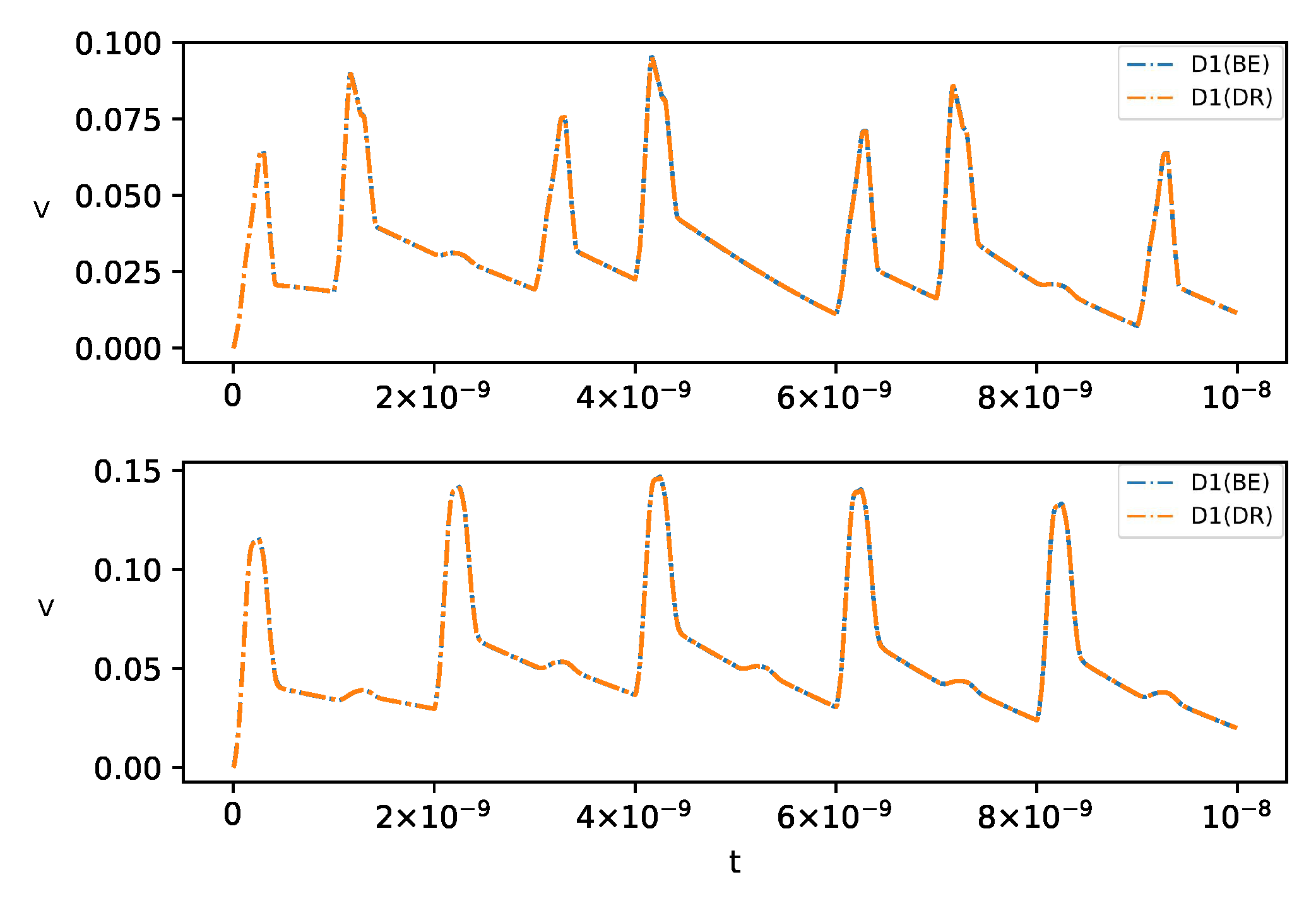
In Figure 4, we compare the transient voltage waveforms simulated by the built-in BE (Backward Euler) method and the EI-DR method combined with the regularization technique. The D1 and D2 cases are used with a fixed time step size $1\times {10}^{-11}$ s. The overlapping agreements confirm that no accuracy loss is caused by the proposed regularization.

5.2. Deflated Restarting Scheme

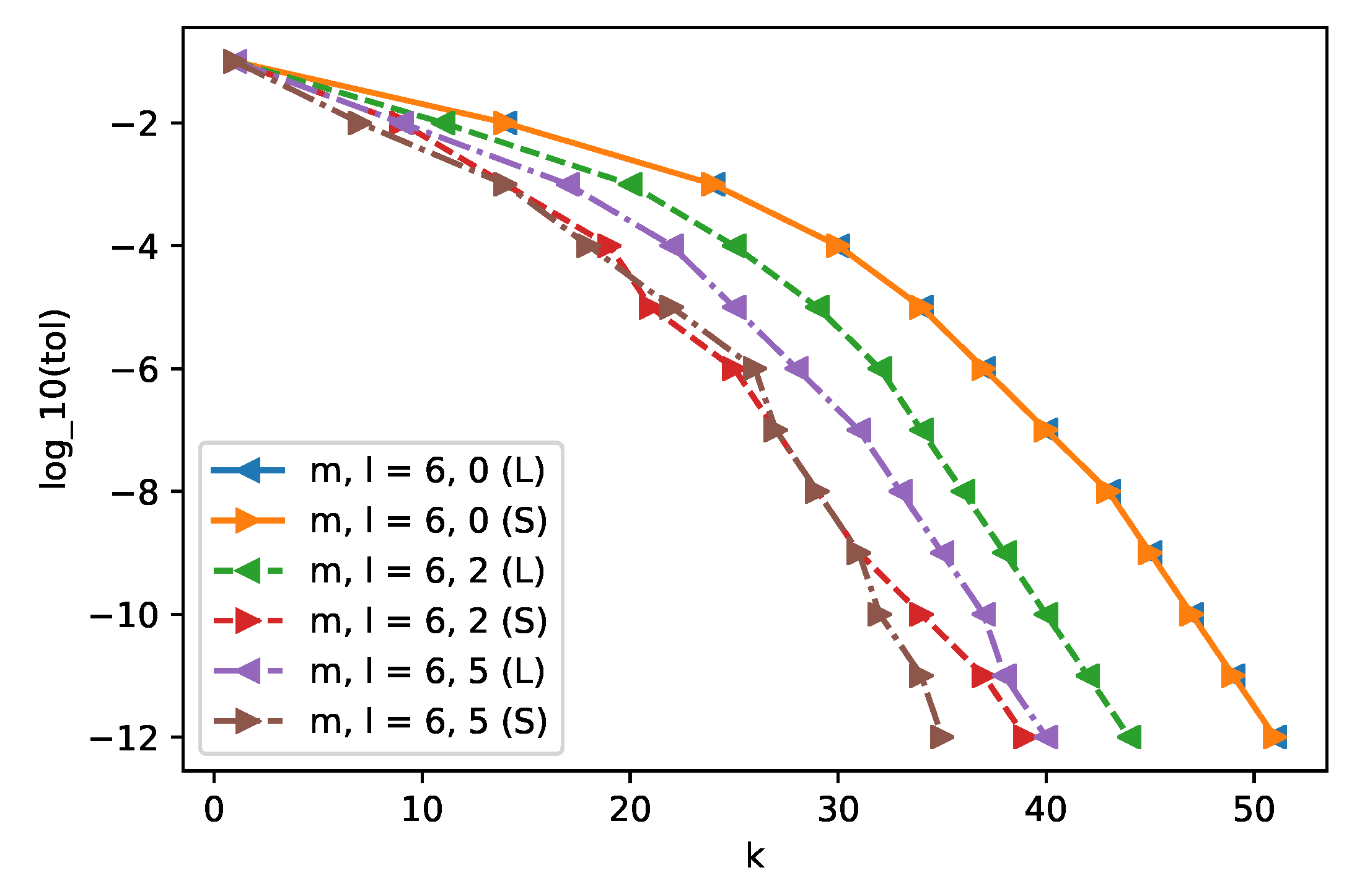
In this section, we investigate the performance of the EI-DR method. As mentioned in Section 4.1, the ordinary Arnoldi process (6) tends to oversample the large-magnitude eigenvalues but undersample the small-magnitude ones that are more pertinent to the final accuracy. Hence, the first question of EI-DR is how to choose the proper eigenvalues (or eigenvectors) of the block Hessenberg matrix $\tilde{H}$ in (41) be to deflated. Below we compare two different choices of the l eigenvalues for deflation. The D1 case in Table 1 is used with a uniform time step size of 0.2 ns for convenience.

Figure 5 shows the convergence history for different settings, where m and l denote the restarting length of the ordinary Krylov subspace and the number of eigenvectors we extract from $\tilde{H}$ for deflation, respectively. The symbol $\left(L\right)$ and $\left(S\right)$ indicate whether we deflate the eigenvectors corresponding to the l largest eigenvalues or the l smallest eigenvalues. The figure plots how the error decreases with the number of restarts k. Note that, when k differs by 1, the corresponding subspace dimension differs by m.

When $l=0$, our deflated restarting scheme coincides with the non-deflated version (EI-R) proposed in Reference [6] and the two curves for $\left(L\right)$ and $\left(S\right)$ overlap in Figure 5 as expected. For nonzero l, however, deflation of the small-magnitude eigenvalues consistently yields faster convergence than that of the large-magnitude eigenvalues, which confirms the analysis in Section 4.1 that slow convergence is due to inadequate sampling of the small eigenvalues. Comparing the curves of $l=2\left(S\right)$ and $l=5\left(S\right)$, one can see that the convergence rates are similar, demonstrating a saturated improvement one could obtain by increasing l. This again suggests that the accuracy is controlled by a fraction of small eigenvalues, and further improvements would be limited if these set of eigenvalues have already been deflated from the new search space. Only for a high accuracy requirement below ${10}^{-9}$, deflating more small eigenvalues is beneficial as shown by the discrepancy at the bottom part of the leftmost two lines.

Table 3. Performance data of D1 and D2.

Tstep = $2\mathbf{\times }{10}^{\mathbf{-}\mathbf{10}}$ s		D1 (${\mathit{m}}_{\mathbf{0}}\mathbf{=}\mathbf{95}$ for No-Restarting)				D2 (${\mathit{m}}_{\mathbf{0}}\mathbf{=}\mathbf{106}$ for No-Restarting)
m	l	k	Spsolve	dim(${\mathit{V}}_{\mathit{km}\mathbf{+}\mathbf{(}\mathit{k}\mathbf{-}\mathbf{1}\mathbf{)}\mathit{l}}$)	Time/s	k	Spsolve	dim(${\mathit{V}}_{\mathit{km}\mathbf{+}\mathbf{(}\mathit{k}\mathbf{-}\mathbf{1}\mathbf{)}\mathit{l}}$)	Time/s
6	0	37	222	222	4.317771	35	210	210	18.117152
	2	25	150	198	2.561108	26	156	206	13.040628
	6	24	144	282	2.513732	22	132	258	10.957821
10	0	17	170	170	2.856241	17	170	170	14.299571
	5	13	130	190	2.194715	12	120	175	10.334383
	10	12	120	230	2.129521	12	120	230	10.400039
14	0	10	140	140	2.624997	11	154	154	12.873702
	8	9	126	190	2.286199	9	126	190	10.665583
	14	8	112	210	2.070850	8	112	210	9.731642

and

Table 4. Performance data of D3 and D4.

Tstep = $\mathbf{1}\times {10}^{-10}$ s		D3 (${\mathit{m}}_0=64$ for No-Restarting)				D4 (${\mathit{m}}_0=73$ for No-Restarting)
m	l	k	Spsolve	dim(${\mathit{V}}_{\mathit{km}+(\mathit{k}-\mathbf{1})\mathit{l}}$)	Time/s	k	Spsolve	dim(${\mathit{V}}_{\mathit{km}+(\mathit{k}-\mathbf{1})\mathit{l}}$)	Time/s
6	0	27	162	162	111.346346	32	192	192	127.529831
	2	20	120	158	84.746398	21	126	166	88.770843
	6	13	78	150	52.377661	15	90	174	59.138819
10	0	12	120	120	80.759488	12	120	120	78.327367
	5	8	80	115	58.257768	9	90	130	62.386851
	10	7	70	130	49.326665	8	80	150	55.504061
14	0	6	84	84	59.579572	7	98	98	66.059572
	8	5	70	102	49.267151	6	84	124	60.321333
	14	5	70	126	49.801739	6	84	154	60.574075

tabulate the performance data of EI-DR for all the four testcases with different combinations of m and l. $spsolve$ denotes the number of triangular solves involved in the Arnoldi process (=km), a main indicator of convergence speed and total runtime. dim($V_{km+(k-1)l}$) is the effective total subspace dimension for EI-DR taking into account the deflated vectors. The l smallest eigenvalues are chosen for deflation. Several observations can be made:

• A higher restarting length m in general leads to faster convergence and reduced runtime, at the cost of a higher memory consumption. Comparing to EI without restarting, EI-R and EI-DR both consume more $spsolve$, indicating a slower convergence.
• For the same m, a higher l typically improves the convergence and reduces $spsolve$. The improvements, however, tend to saturate after a certain value of l. For instance, for the case D2 with $m=10$, using $l=5$ or $l=10$ results in the same number of restarting k, suggesting a higher l is not always optimal for a particular m.
• Comparing to EI-R ($l=0$), EI-DR reduces number of $spsolve$ by ratios between $30\%$ to $50\%$ across different cases and various m, confirming that the proposed EI-DR is an effective acceleration scheme. The improvement is more significant for small m than for large m.

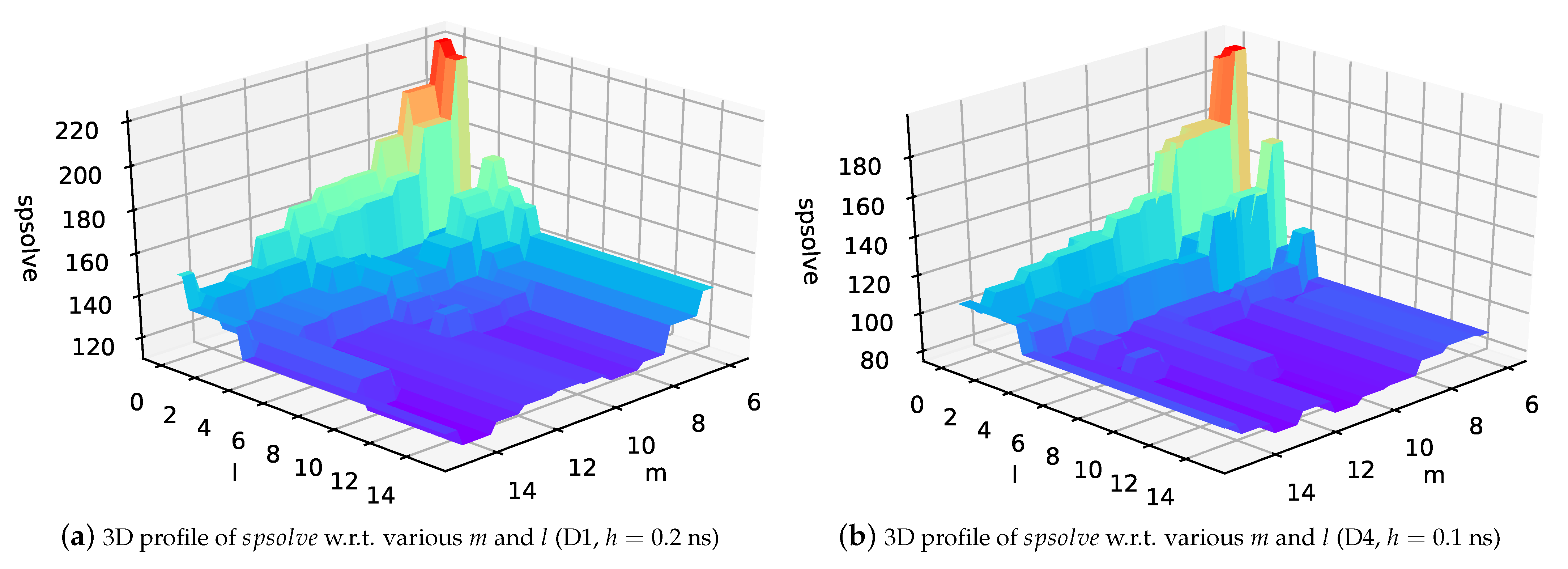
Finally, we plot the 3D profiles of the number of $spsolve$ with respect to different $(m,l)$ pairs for D1 and D4 in Figure 6a,b, respectively. m varies from 6 to 14, and l varies from 0 to m. In the two figures, the peaks are both at $(6,0)$, and the valleys are near $(14,14)$, which is consistent with our analysis above. The optimal selection of m and l in practice is generally a trade-off between runtime and memory.

• extract l eigenvectors corresponding to the largest-magnitude eigenvalues of $\tilde{H}$.
• extract l eigenvectors corresponding to the smallest-magnitude eigenvalues of $\tilde{H}$.

6. Conclusions

In this paper, we proposed two techniques to improve EI based on the ordinary Krylov subspace for linear circuits. We firstly propose an implicit regularization technique for the ordinary Krylov subspace EI to solve the singular C problem. This regularization is computationally efficient and sparsity preserving. Next, we analyze the convergence problems with the ordinary Krylov subspace and the simple restarting scheme for stiff circuits. Based on the analysis, we then develop a deflated restarting scheme that deflates a carefully chosen region of the matrix spectrum to accelerate the convergence. Numerical results demonstrate the effectiveness of our regularization technique, and the substantial convergence improvement arising from the proposed deflated restarting scheme for stiff circuits. The optimal, even adaptive, selection of m and l in our deflated restarting scheme will be a topic for future investigation.

References

- Chen, Q.; Schoenmaker, W. A new tightly-coupled transient electro-thermal simulation method for power electronics. In Proceedings of the IEEE/ACM International Conference on Computer-Aided Design (ICCAD), Austin, TX, USA, 7–10 November 2016; pp. 1–7. [Google Scholar]
- Chen, Q.; Schoenmaker, W.; Weng, S.H.; Cheng, C.K.; Chen, G.H.; Jiang, L.J.; Wong, N. A fast time-domain EM-TCAD coupled simulation framework via matrix exponential. In Proceedings of the IEEE/ACM International Conference on Computer-Aided Design (ICCAD), San Diego, CA, USA, 5–8 November 2012; pp. 422–428. [Google Scholar]
- Caliari, M.; Vianello, M.; Bergamaschi, L. Interpolating discrete advection–diffusion propagators at Leja sequences. J. Comput. Appl. Math. 2004, 172, 79–99. [Google Scholar] [CrossRef] [Green Version]
- Chen, P.; Cheng, C.; Park, D.; Wang, X. Transient circuit simulation for differential algebraic systems using matrix exponential. In Proceedings of the IEEE/ACM International Conference on Computer-Aided Design ICCAD, San Diego, CA, USA, 5–8 November 2018; p. 99. [Google Scholar]
- Chen, Q.; Weng, S.; Cheng, C. A Practical Regularization Technique for Modified Nodal Analysis in Large-Scale Time-Domain Circuit Simulation. IEEE Trans. Comput.-Aided Des. Integr. Circuits Syst. 2012, 31, 1031–1040. [Google Scholar] [CrossRef] [Green Version]
- Weng, S.H.; Chen, Q.; Wong, N.; Cheng, C.K. Circuit simulation via matrix exponential method for stiffness handling and parallel processing. In Proceedings of the IEEE/ACM International Conference on Computer-Aided Design (ICCAD), San Jose, CA, USA, 5–8 November 2012; pp. 407–414. [Google Scholar]
- Weng, S.H.; Chen, Q.; Cheng, C.K. Time-Domain Analysis of Large-Scale Circuits by Matrix Exponential Method With Adaptive Control. IEEE Trans. Comput.-Aided Des. Integr. Circuits Syst. 2012, 31, 1180–1193. [Google Scholar] [CrossRef] [Green Version]
- Zhuang, H.; Weng, S.H.; Cheng, C.K. Power Grid Simulation using Matrix Exponential Method with Rational Krylov Subspaces. In Proceedings of the IEEE 9th International Conference on ASIC (ASICON), Shenzhen, China, 28–31 October 2013; pp. 369–372. [Google Scholar]
- Zhuang, H.; Weng, S.H.; Lin, J.H.; Cheng, C.K. MATEX: A Distributed Framework for Transient Simulation of Power Distribution Networks. In Proceedings of the IEEE/ACM Design Automation Conference (DAC), San Francisco, CA, USA, 1–5 June 2014; pp. 81:1–81:6. [Google Scholar] [CrossRef] [Green Version]
- Zhuang, H.; Yu, W.; Kang, I.; Wang, X.; Cheng, C.K. An Algorithmic Framework for Efficient Large-scale Circuit Simulation Using Exponential Integrators. In Proceedings of the IEEE/ACM Design Automation Conference (DAC), San Francisco, CA, USA, 7–11 June 2015; pp. 163:1–163:6. [Google Scholar]
- Zhuang, H.; Yu, W.; Weng, S.; Kang, I.; Lin, J.; Zhang, X.; Coutts, R.; Cheng, C. Simulation Algorithms With Exponential Integration for Time-Domain Analysis of Large-Scale Power Delivery Networks. IEEE Trans. Comput. Aided Des. Integr. Circuits Syst. 2016, 35, 1681–1694. [Google Scholar] [CrossRef] [Green Version]
- Chen, Q.; Zhao, W.; Wong, N. Efficient matrix exponential method based on extended Krylov subspace for transient simulation of large-scale linear circuits. In Proceedings of the 2014 19th Asia and South Pacific Design Automation Conference (ASP-DAC), Singapore, 20–23 January 2014; pp. 262–266. [Google Scholar] [CrossRef] [Green Version]
- Zhang, M.; Li, J.; Chen, O. Deflated Restarting of Exponential Integrator Method for Efficient Transient Circuit Simulation. In Proceedings of the 2020 IEEE 15th International Conference on Solid-State & Integrated Circuit Technology (ICSICT), Kungming, China, 3–6 November 2020; pp. 1–4. [Google Scholar] [CrossRef]
- Cameron, S.H. Piecewise Linear Approximations. In IIT Research Institute Technical Report No. CSTN-106; IIT Research Institute Press: Chicago, IL, USA, 1966. [Google Scholar]
- Al-Mohy, A.H.; Higham, N.J. Computing the Action of the Matrix Exponential with an Application to Exponential Integrators. SIAM J. Sci. Comput. 2011, 33, 488–511. [Google Scholar] [CrossRef]
- Saad, Y. Analysis of some Krylov subspace approximations to the matrix exponential operator. SIAM J. Numer. Anal. 1992, 29, 209–228. [Google Scholar] [CrossRef]
- Chua, L.O.; Lin, P.M. Computer-Aided Analysis of Electronic Circuits; Prentice-Hall: Hoboken, NJ, USA, 1975. [Google Scholar]
- Schwarz, D.; Tischendorf, C. Structural analysis of electric circuits and consequences for MNA. Int. J. Circuit Theory Appl. 2000, 28, 131–162. [Google Scholar] [CrossRef]
- Ilchmann, A.; Reis, T. Surveys in Differential-Algebraic Equations; Springer International Publishing: New York, NY, USA, 2015. [Google Scholar] [CrossRef]
- Il’in, V. Projection Methods in Krylov Subspaces. J. Math. Sci. 2019, 240, 772–782. [Google Scholar] [CrossRef]
- Eiermann, M.; Ernst, O. A Restarted Krylov Subspace Method for the Evaluation of Matrix Functions. SIAM J. Numer. Anal. 2006, 44, 2481–2504. [Google Scholar] [CrossRef] [Green Version]
- Gaul, A. Recycling Krylov Subspace Methods for Sequences of Linear Systems. Ph.D. Thesis, Analysis and Applications University of Erlangen, Berlin, Germany, 2014. [Google Scholar] [CrossRef]
- Eiermann, M.; Ernst, O.; Güttel, S. Deflated Restarting for Matrix Functions. SIAM J. Matrix Anal. Appl. 2011, 32, 621–641. [Google Scholar] [CrossRef] [Green Version]
- Venturini, G. Ahkab: An Open-Source SPICE-Like Interactive Circuit Simulator. 2015. Available online: https://ahkab.readthedocs.io/en/latest/ (accessed on 21 March 2021).
Figure 1.
Typical RLC circuit and its MNA equations.
Figure 2.
Flow of the proposed regularization.
Figure 3.
Sampling regions of spectrum in ordinary Krylov subspace methods.
Figure 4.
Voltage waveform comparisons between BE and EI-DR for D1 and D2.
Figure 5.
Convergence comparison between two different selections of eigenvalues to be deflated in EI-DR. (L) refers largest-magnitude eigenvalues, (S) refers to smallest-magnitude eigenvalues. The D1 case is used with a fixed time step 0.2 ns.