A Topology Analysis-Based MMC-HVDC Grid Transmission Capacity Calculation Method

Abstract

Modular multilevel converter-based high voltage direct current (MMC-HVDC) has a broad application prospect in renewable energy transmission. With the development of converter capacity, the transmission capacity calculation for MMC-HVDC grids becomes important for power dispatching. The existing method depends on manual work and is suitable for a simple grid. However, as the grid structure and operation modes become more and more complex, it becomes difficult to calculate the transmission capacity of different operation modes for an MMC-HVDC grid. This paper analyzed and simplified affecting factors and basic topologies. On this basis, a topology-based MMC-HVDC grid transmission capacity calculation method is proposed. First, an MMC-HVDC grid is divided into sending end grid, transmission section lines, and receiving end grid. Then the power limits of these three parts are calculated. Finally, the transmission capacity is determined by analyzing the connection mode of these three parts. This method can be adapted to any kind of MMC-HVDC grid and can be easily programmed.

1. Introduction

Modular multilevel converter-based high voltage direct current (MMC-HVDC) has a broad application prospect in renewable energy transmission due to its lack of commutation failure and other advantages [1,2,3,4]. China has built the first MMC-HVDC project with a grid structure, the Zhangbei MMC-HVDC project [5,6]. It also has the highest voltage level and the biggest converter capacity among MMC-HVDC projects in the world [7]. The MMC-HVDC grid transmission capacity is the maximum power transmitted from the generating plant to the load grid through the MMC-HVDC grid. It is increasing in newly built projects and cannot be ignored in power grid operating control. Therefore, it is important to calculate the transmission capacity of the MMC-HVDC grid when the electric power dispatch center (EPDC) arranges the operation mode of the power grid. Furthermore, the MMC-HVDC grid transmission capacity is an important consideration in formulating a control and protection strategy.

For AC grids, the transmission capacity is usually used to describe a transmission section, and the transmission capacity is usually determined by the thermal stability limit of transmission lines and the static stability limit of the transmission section [8,9]. Many studies have investigated how to increase the transmission capacity of the AC grid [10,11]. For MMC-HVDC grids, previous studies have mainly focused on the safe and stable operation area of a single converter station [12,13]. There is no special calculation method for MMC-HVDC grid transmission capacity calculation. In practice projects, the transmission capacity calculation of different operation modes adopts the calculation method of the AC grid transmission section and depends on manual work. However, with the development of MMC-HVDC, the topology and operation modes are more and more complex. For example, the Zhangbei MMC-HVDC project has four converter stations and 5928 possible operation modes [14]. It is difficult to finish the calculation by manual work, not to mention the more complex topologies that may exist in the future. Therefore, it is necessary to study the transmission capacity calculation method for the complex topology of MMC-HVDC grids.

This paper focuses on the calculation method of transmission capacity suitable for different topologies of MMC-HVDC. First, the main factors that affect the transmission capacity in MMC-HVDC grids are proposed. Next, the typical topology of MMC-HVDC grids is analyzed and the node types are divided. On this basis, this paper simplifies the affecting factors and defines the transmission section of the sending and receiving end. Then, a calculation method is proposed by combining the transmission capacity of the sending end, receiving end, and section. The proposed method can be applied to different MMC-HVDC topologies and can be programmed.

2. Main Factors Affecting Transmission Capacity

The main factors that affect transmission capacity can be divided into two categories. One is determined by the current and voltage limit of the device and is usually shown as rated power. The other is the maximum operating power determined by the demand for safe and stable operation of the power grid, which is usually shown as the safe and stable operation area of the converter station.

2.1. Rated Power Limits

Each device in the MMC-HVDC grid has a rated power limit. Among them, the rated power of three kinds of devices has the greatest impact on the transmission capacity: protection devices like DC circuit breakers (DCB), converters, and transmission lines. For DCBs, the rated power affects the realization of its basic function of breaking the circuit to isolate faults [15]. For converters, the rated power is related to the current and voltage limit of internal components like capacitors, and for transmission lines, the rated power limit is usually equal to their thermal stability limit. Once the actual operation is greater than the rated power limits of these devices, the safety of MMC-HVDC is threatened.

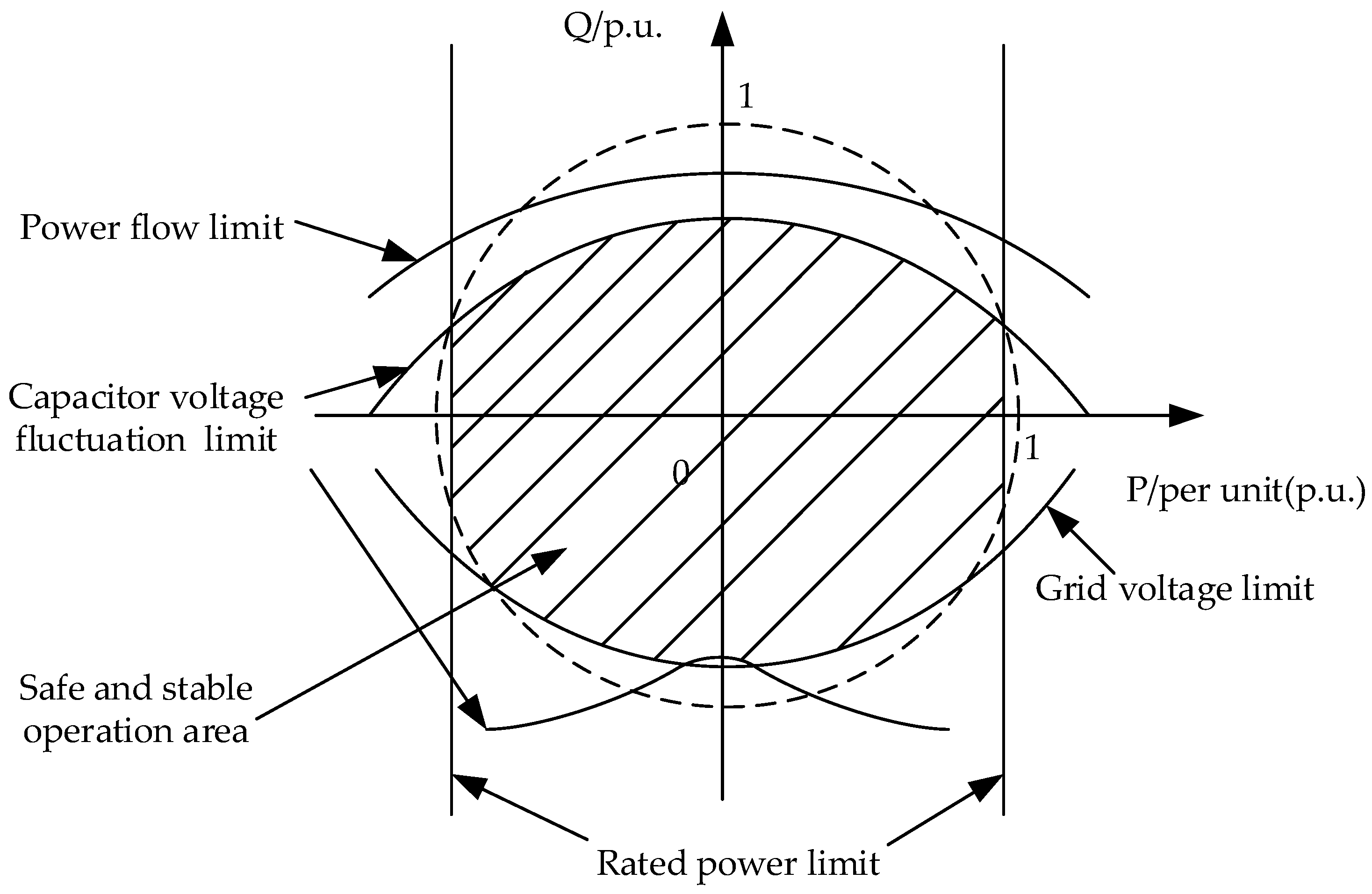
2.2. Safe and Stable Operation Area of a Converter Station

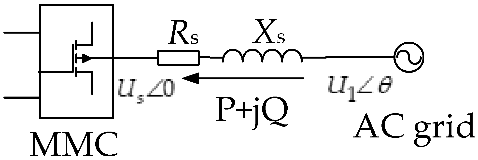
A simple schematic diagram of MMC connected to the AC system is shown in Figure 1, where U_s∠0 is the voltage of the point of common coupling (PCC), U₁∠θ is the voltage of the AC grid, R_s, and X_s denotes the resistance and reactance for transmission lines.

The power flow from MMC to the AC grid is calculated as Equation (1).

$$U_1\angle \theta -U_{\mathrm{s}}\angle 0=\frac{P{R}_{\mathrm{s}}+Q{X}_{\mathrm{s}}}{U_{\mathrm{s}}}+\mathrm{j}\frac{P{X}_{\mathrm{s}}-Q{R}_{\mathrm{s}}}{U_{\mathrm{s}}}$$

(1)

From (1), the voltage change can be shown as (2).

$$\{\begin{array}{l}{U}_1\cos \theta -U_{\mathrm{s}}=\frac{P{R}_{\mathrm{s}}+Q{X}_{\mathrm{s}}}{U_{\mathrm{s}}}\\ U_1\sin \theta =\frac{P{X}_{\mathrm{s}}-Q{R}_{\mathrm{s}}}{U_{\mathrm{s}}}\end{array}$$

(2)

Form (2), the PCC voltage can be calculated by (3).

$$\{\begin{array}{l}{U}_{\mathrm{s}}^4+(2a-U_1^2)U_{\mathrm{s}}^2+a^2+b^2=0\\ a=P{R}_{\mathrm{s}}+Q{X}_{\mathrm{s}}, b=P{X}_{\mathrm{s}}-Q{R}_{\mathrm{s}}\end{array}$$

(3)

To make sure (3) has a real solution, (4) needs to be satisfied.

$$\{\begin{array}{l}{(2a-U_1^2)}^2-4(a^2+b^2)\ge 0\\ U_1^2-2a+\sqrt{{(2a-U_1^2)}^2-4(a^2+b^2)}\ge 0\end{array}$$

(4)

From (4), the power flow limit for the MMC output active power and reactive power is obtained, which is a basic limit of the safe and stable operation area of a converter station.

Furthermore, there are other limits to form the safe and stable operation area of a converter station, such as the voltage modulation limit, capacitor voltage fluctuation limit, and grid voltage limit. A typical safe and stable operation area of a converter station form [13] is shown in Figure 2.

3. MMC-HVDC Grid Topology Analysis

In order to calculate the transmission capacity of various grid structures and multiple operation modes, this paper adopts a calculation method based on topology analysis.

3.1. Basic Topology of a MMC-HVDC Grid

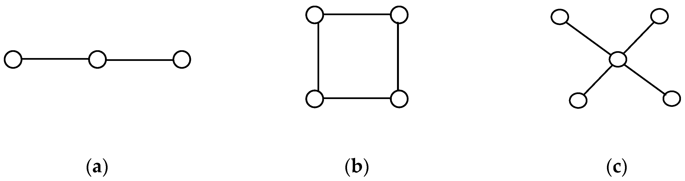
There are three basic topologies of a MMC-HVDC grid as shown in Figure 3, where each converter station is represented as a node and each transmission line is represented as a single line. In a loop grid, each station is connected to two stations, and in a star grid, there is at least one station connected to more than two stations.

3.2. Node Type Classification

According to the power flow direction, grid nodes can be divided into three types: the sending nodes, the receiving nodes, and the adjustment nodes. The sending nodes are connected to the power sources like wind farms or other plants that need to send power through MMC-HVDC. The receiving nodes are connected to the load center that receives power from MMC-HVDC. To keep the power balance and voltage stability in the DC grid, there needs to be one converter that works at DC voltage constant control mode for an MMC-HVDC grid [16], which is defined as the adjustment node.

The power of sending nodes flows from the AC grid to the DC grid and the power of receiving nodes flows from the DC grid to the AC grid. The power flow of adjustment nodes can be in both directions.

4. Transmission Capacity Calculation Method

Since the topology and operation mode of the MMC-HVDC grid can be quite complex, it is necessary to simplify the grid and limit factors.

4.1. Main Factors Simplification

The protection devices can be divided into station protection and line protection. Thus, the station protection rated power limit can combine with the safe and stable operation area of the converter station and the line protection rated power limit can combine with the transmission line rated power limit. Therefore, the main factors are simplified to two factors: station limit P_s and line limit P_l, which can be obtained by (5):

$$\{\begin{array}{l}{P}_{\mathrm{s}}=\min (P_{\mathrm{st}},P_{\mathrm{sp}})\\ P_{\mathrm{l}}=\min (P_{\mathrm{tl}},P_{\mathrm{lp}})\end{array}$$

(5)

In (5), P_st is the maximum power of the safe and stable operation area of the converter station, P_sp is the rated power limit of station protection, P_tl is the rated power limit of the transmission line and P_lp is the rated power limit of the line protection.

4.2. Topology Simplification

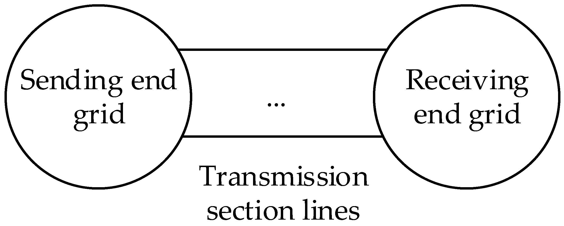
Combine all the sending nodes and lines between them in an MMC-HVDC grid, a sending end grid is formed. Similarly, a receiving end grid can be formed. Meanwhile, the adjustment node can be treated as a sending node and receiving node, so it needs to be calculated twice. Then the transmission lines between sending nodes and receiving nodes are combined, and a group of transmission section lines is formed. In this way, every kind of MMC-HVDC grid can be simplified to an end-to-end grid as shown in Figure 4.

For an end-to-end grid, the transmission capacity can be easily obtained by (6):

$$P_{\max }=\min (P_{\mathrm{sen}},P_{\mathrm{rec}},P_{\sec })$$

(6)

where P_sen is the maximum output power of the sending end grid, P_rec is the maximum input power of the receiving end grid and P_sec is the maximum transmission power of section lines.

In this way, the calculation of a complex grid is simplified to three maximum power calculations.

4.3. MMC-HVDC Transmission Capacity Calculation Method

4.3.1. Calculation Preparation

For a bipolar MMC-HVDC grid, two poles can operate independently. Thus, the transmission capacity can be calculated separately too. The calculation method in this paper is developed for a single pole, so the bipolar grid capacity can be obtained by adding the calculated results of two poles.

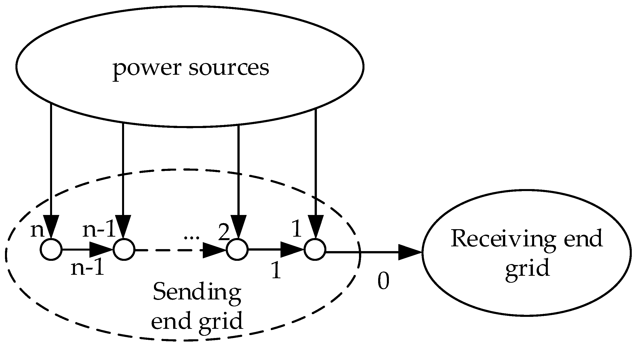
For the convenience of calculation, the nodes and lines of the sending end grid and receiving end grid are numbered separately. The transmission section lines are the start line, known as line 0, and all the sending nodes and receiving nodes connected to transmission section lines are numbered as 1. Then, the sending nodes and receiving nodes connected to nodes 1 are numbered as 2, and so on until all the nodes in the grid are numbered. The line number is determined by the smaller node number at both ends of the line. For example, the transmission line between node 1 and node 2 is line 1. Usually, the biggest number is represented as n.

To obtain a higher output power, after numbering the power grid nodes, the power should flow from nodes of larger numbers to nodes of smaller numbers. Therefore, the power flow direction is determined.

4.3.2. Maximum Output Power of Basic Topologies

Take the sending end grid as an example, the calculation method of the maximum output power of different topologies is as follows.

For a single chain grid, as shown in Figure 5, there are n nodes in the sending end grid and each node has an input power from power sources. The maximum input power can be calculated by (5) and is equal to P_s.

All the P_s and P_l are numbered according to the node number and line number. P_j,j-1 (j = 2,3…n) represents the maximum transmission power between nodes. Thus, the maximum output power of the sending end grid can be calculated by (7):

$$\{\begin{array}{l}{P}_{\mathrm{n},\mathrm{n}-1}=\min (P_{\mathrm{sn}},P_{\ln -1})\\ P_{\mathrm{n}-1,\mathrm{n}-2}=\min (P_{\mathrm{sn}-1}+P_{\mathrm{n},\mathrm{n}-1},P_{\ln -2})\\ \dots \\ P_{2,1}=\min (P_{\mathrm{s}2}+P_{3,2},P_{\mathrm{l}1})\\ P_{\mathrm{sen}}=P_{2,1}+P_{\mathrm{s}1}\end{array}$$

(7)

This equation is an iterative process and is easy to program.

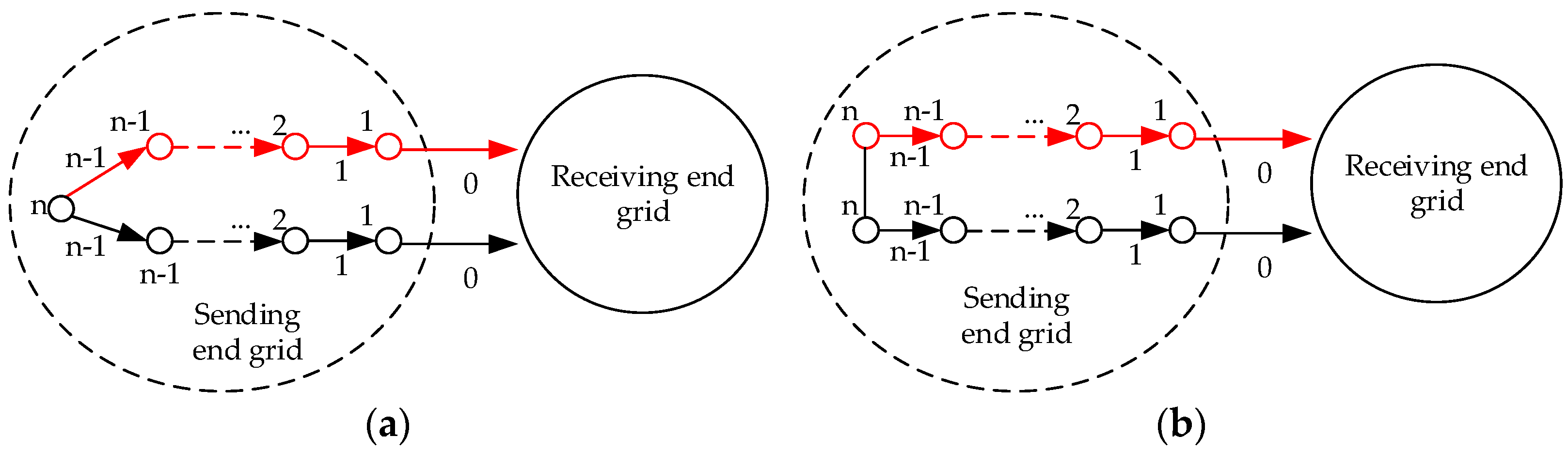
For a loop grid, according to the parity of the number of sending nodes, there are two different types of loop grids as shown in Figure 6. If the sending node’s number is odd, there is only one node n. Otherwise, there are two nodes n.

In Figure 6, a loop grid can be divided into two chains as long as P_n,n−1 is determined. For a grid like Figure 6a, P_n,n−1 can be calculated by (8).

When the sum of the power limit of two lines n−1 is greater than P_sn, all the output power of node n can be transmitted to node n−1. If the power limit of both lines is greater than half of P_sn, P_n,n−1 of two lines n−1 can both be half of P_sn. If the power limit of one line n−1 is smaller than half of P_sn, P_n,n−1 of this line will be the power limit of this line, and the rest power of node n will be transmitted through the other one.

When the sum of the power limit of two lines n−1 is smaller than P_sn, the output power of node n cannot be fully transmitted to node n−1. Therefore P_n,n−1 will be the power limit of each line.

$$\{\begin{array}{l}{P}_{\mathrm{n},\mathrm{n}-1}(r)=P_{\mathrm{n},\mathrm{n}-1}(b)=\frac{1}{2}{P}_{\mathrm{sn}},\mathrm{when} P_{\ln -1}(r)\ge \frac{1}{2}{P}_{\mathrm{sn}},P_{\ln -1}(b)\ge \frac{1}{2}{P}_{\mathrm{sn}}\\ P_{\mathrm{n},\mathrm{n}-1}(r)=P_{\mathrm{sn}}-P_{\ln -1}(b),P_{\mathrm{n},\mathrm{n}-1}(b)=P_{\ln -1}(b),\mathrm{when} P_{\ln -1}(r)+P_{\ln -1}(b)\ge P_{\mathrm{sn}},P_{\ln -1}(b)\le \frac{1}{2}{P}_{\mathrm{sn}}\\ P_{\mathrm{n},\mathrm{n}-1}(r)=P_{\ln -1}(r),P_{\mathrm{n},\mathrm{n}-1}(b)=P_{\mathrm{sn}}-P_{\ln -1}(r),\mathrm{when} P_{\ln -1}(r)+P_{\ln -1}(b)\ge P_{\mathrm{sn}},P_{\ln -1}(r)\le \frac{1}{2}{P}_{\mathrm{sn}}\\ P_{\mathrm{n},\mathrm{n}-1}(r)=P_{\ln -1}(r),P_{\mathrm{n},\mathrm{n}-1}(b)=P_{\ln -1}(b),\mathrm{when} P_{\ln -1}(r)+P_{\ln -1}(b)\le P_{\mathrm{sn}}\end{array}$$

(8)

Symbol (r) represents variables in the red chain and (b) represents variables in the black chain in Figure 6.

For a grid like Figure 6b, P_n,n−1 can be calculated by (9).

When the power limit of both lines n−1 is greater than the power limit of the node n it is connected to, the output power of both node n can be fully transmitted, and P_n,n−1 will be the power limit of each node n.

When the sum of the power limit of two lines n−1 is greater than the sum of the power limit of two nodes n, but the power limit of one line n−1 is smaller than the power limit of the node n that it is connected to, P_n,n−1 of this line will be the power limit of this line and the remaining power of this node n will be transmitted through line n. To avoid confusion, this node is called n1 and the other node is called n2. If the power limit of line n is greater than the remaining power of node n1, the remaining power can be fully transmitted from node n1 to node n2 and then transmitted through line n−1. Otherwise, power from node n1 to node n2 is the power limit of line n, and the conditions of the sum of the power limit of two lines n−1 for this situation can be changed.

When the power limit of both line n−1 is smaller than the power limit of the node n it is connected to, P_n,n−1 will be the power limit of each line n−1.

$$\{\begin{array}{c}{P}_{\mathrm{n},\mathrm{n}-1}(r)=P_{\mathrm{sn}}(r),P_{\mathrm{n},\mathrm{n}-1}(b)=P_{\mathrm{sn}}(b),\mathrm{when} P_{\ln -1}(r)\ge P_{\mathrm{sn}}(r),P_{\ln -1}(b)\ge P_{\mathrm{sn}}(b)\\ P_{\mathrm{n},\mathrm{n}-1}(r)=P_{\mathrm{sn}}(r)+P_{\mathrm{sn}}(b)-P_{\ln -1}(b),P_{\mathrm{n},\mathrm{n}-1}(b)=P_{\ln -1}(b),\mathrm{when} P_{\ln -1}(r)+P_{\ln -1}(b)\ge P_{\mathrm{sn}}(r)+P_{\mathrm{sn}}(b)\\ \mathrm{and} P_{\ln -1}(b)\le P_{\mathrm{sn}}(b),P_{\ln }\ge P_{\mathrm{sn}}(b)-P_{\ln -1}(b)\\ P_{\mathrm{n},\mathrm{n}-1}(r)=P_{\ln -1}(r),P_{\mathrm{n},\mathrm{n}-1}(b)=P_{\mathrm{sn}}(r)+P_{\mathrm{sn}}(b)-P_{\ln -1}(r),\mathrm{when} P_{\ln -1}(r)+P_{\ln -1}(b)\ge P_{\mathrm{sn}}(r)+P_{\mathrm{sn}}(b)\\ \mathrm{and} P_{\ln -1}(r)\le P_{\mathrm{sn}}(r),P_{\ln }\ge P_{\mathrm{sn}}(r)-P_{\ln -1}(r)\\ \begin{array}{c}{P}_{\mathrm{n},\mathrm{n}-1}(r)=P_{\mathrm{sn}}(r)+P_{\ln },P_{\mathrm{n},\mathrm{n}-1}(b)=P_{\ln -1}(b),\mathrm{when} P_{\ln -1}(r)\ge P_{\mathrm{sn}}(r)+P_{\ln }\\ \mathrm{and} P_{\ln -1}(b)\le P_{\mathrm{sn}}(b),P_{\ln }\le P_{\mathrm{sn}}(b)-P_{\ln -1}(b)\\ P_{\mathrm{n},\mathrm{n}-1}(r)=P_{\ln -1}(r),P_{\mathrm{n},\mathrm{n}-1}(b)=P_{\mathrm{sn}}(r)+P_{\ln },\mathrm{when} P_{\ln -1}(r)\le P_{\mathrm{sn}}(r)\\ \mathrm{and} P_{\ln -1}(b)\ge P_{\mathrm{sn}}(b)+P_{\ln },P_{\ln }\le P_{\mathrm{sn}}(r)-P_{\ln -1}(r)\end{array}\\ P_{\mathrm{n},\mathrm{n}-1}(r)=P_{\ln -1}(r),P_{\mathrm{n},\mathrm{n}-1}(b)=P_{\ln -1}(b),\mathrm{when} P_{\ln -1}(r)\le P_{\mathrm{sn}}(r),P_{\ln -1}(b)\le P_{\mathrm{sn}}(b)\end{array}$$

(9)

P_ln is the line limit between red node n and black node n.

Taking (8) or (9) into (7) and calculating the maximum output power of the red chain and the black chain separately gives the maximum output power of a loop grid.

For a star grid, the node connecting to more than two nodes is called the center node and the center node number is m. Thus P_m,m−1 can be calculated by (10):

$$P_{\mathrm{m},\mathrm{m}-1}=\min (P_{\mathrm{sm}}+P_{\mathrm{m}+1,\mathrm{m}}(1)+P_{\mathrm{m}+1,\mathrm{m}}(2)+\dots +P_{\mathrm{m}+1,\mathrm{m}}(\mathrm{c}),P_{\mathrm{l}\mathrm{m}-1})$$

(10)

Symbol (1),(2)…(c) represent multiple lines between node m and node m+1, c is the total number of node m+1.

Taking (10) into (7) gives the maximum output power of a star grid. Therefore, the maximum output power of three basic MMC-HVDC grid topologies can be calculated, and the maximum input power of the receiving end grid can be calculated in the same way.

4.3.3. Transmission Capacity Calculation

Usually, the transmission capacity can be calculated by (6). However, it is worth noting that the sending end grid and receiving end grid may contain independent sub-grids. As a result, the calculation method needs to be refined. The method is to calculate the maximum power of each transmission section line and add all the results.

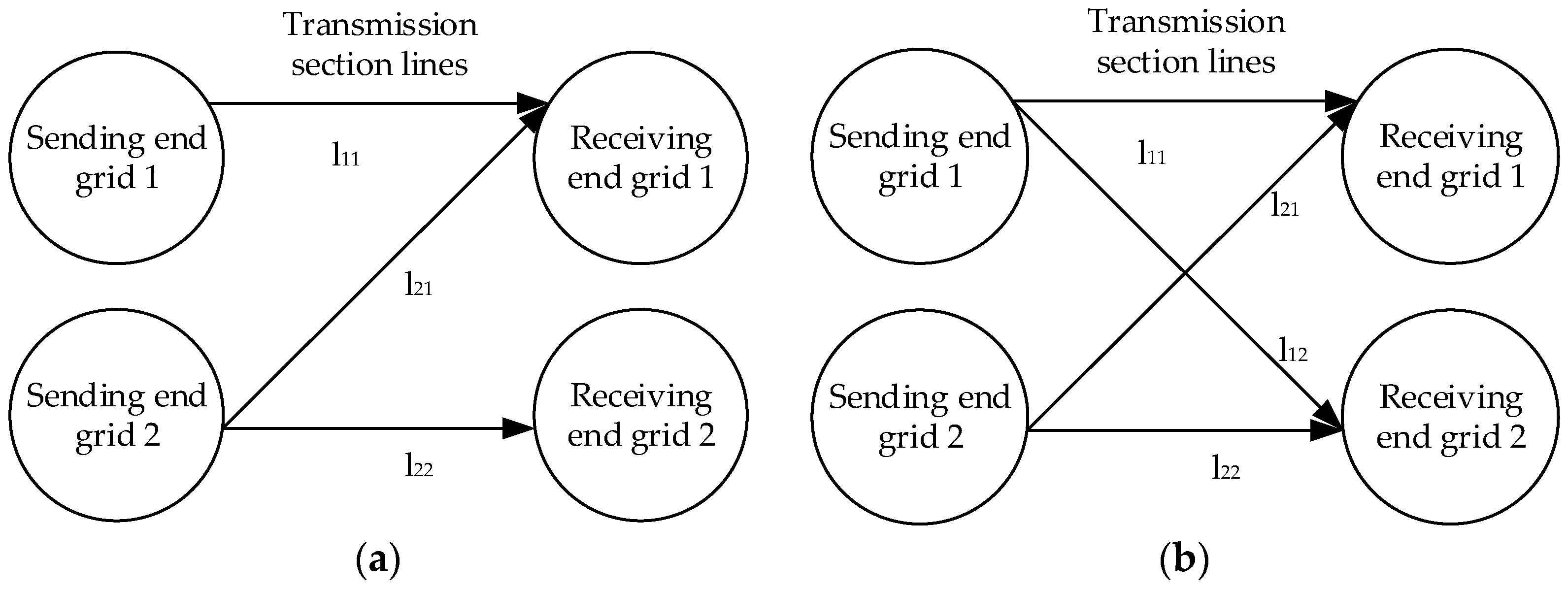
Take two sub-grids as an example, there are two kinds of connecting modes between grids as shown in Figure 7. When a receiving end grid is only connected to one sending end grid, the connection mode is called the “Z” mode in this paper. And when both receiving end grids are connected to both sending end grids, the connection mode is called the “X” mode.

First, the minimum limit of sub-grids and transmission section lines is found. If it is a sending end grid, then the number of this sending end grid will be 1. Then, the receiving end grids connected to sending end grid 1 are sorted by the value of their maximum receiving power from 1 to i, where i is the number of receiving end grids connected to sending end grid 1. Next, the sending end grids connected to receiving end grid 1 are sorted by the value of their maximum output power from 2 to j, where j-1 is the number of sending end grids connected to the receiving end grid 1. Then, the receiving end grids connected to sending end grid 2 are sorted by the value of their maximum receiving power from i+1… Through this cross-numbering method, all sub-grids can be numbered.

If the minimum limit is the limit of a receiving end grid, the numbering method will be similar and only needs to start from receiving end grid 1. If the minimum limit is the limit of a transmission section line, the sending end grid and receiving end grid are numbered as sending end grid 1 and receiving end grid 1 first, and then the follow step will be the same.

Therefore, the transmission capacity of the MMC-HVDC grid can be obtained by adding the transmission capacities of each transmission section line in order. In the calculation of each line, it is necessary to subtract the capacity occupation of the sending end grids and receiving end grids of previous sections. For the “Z” mode, the transmission capacity can be calculated by (11):

$$\{\begin{array}{l}{P}_{\max }=P_{\max 11}+P_{\max 21}+P_{\max 22}\\ P_{\max 11}=\min (P_{\mathrm{sen}1},P_{\mathrm{r}ec1},P_{{\mathrm{l}}_{11}})\\ P_{\max 21}=\min (P_{\mathrm{sen}2},P_{\mathrm{r}ec1}-P_{\max 11},P_{{\mathrm{l}}_{21}})\\ P_{\max 22}=\min (P_{\mathrm{sen}2}-P_{\max 21},P_{\mathrm{r}ec2},P_{{\mathrm{l}}_{22}})\end{array}$$

(11)

The footmark represents the number of the grid and line. Similarly, for “X” mode, the transmission capacity can be calculated by (12):

$$\{\begin{array}{l}{P}_{\max }=P_{\max 11}+P_{\max 12}+P_{\max 21}+P_{\max 22}\\ P_{\max 11}=\min (P_{\mathrm{sen}1},P_{\mathrm{r}ec1},P_{{\mathrm{l}}_{11}})\\ P_{\max 12}=\min (P_{\mathrm{sen}1}-P_{\max 11},P_{\mathrm{r}ec2},P_{{\mathrm{l}}_{12}})\\ P_{\max 21}=\min (P_{\mathrm{sen}2},P_{\mathrm{r}ec1}-P_{\max 11},P_{{\mathrm{l}}_{21}})\\ P_{\max 22}=\min (P_{\mathrm{sen}2}-P_{\max 21},P_{\mathrm{r}ec2}-P_{\max 12},P_{{\mathrm{l}}_{22}})\end{array}$$

(12)

For grids with more than two sub-grids, the calculation method is similar, except that the capacity needed to be subtracted is a little different.

Therefore, the MMC-HVDC grid transmission capacity can be obtained by (5) to (12). These equations contain a lot of iteration and comparative calculation. As a result, they are easy to program by computers.

5. Examples

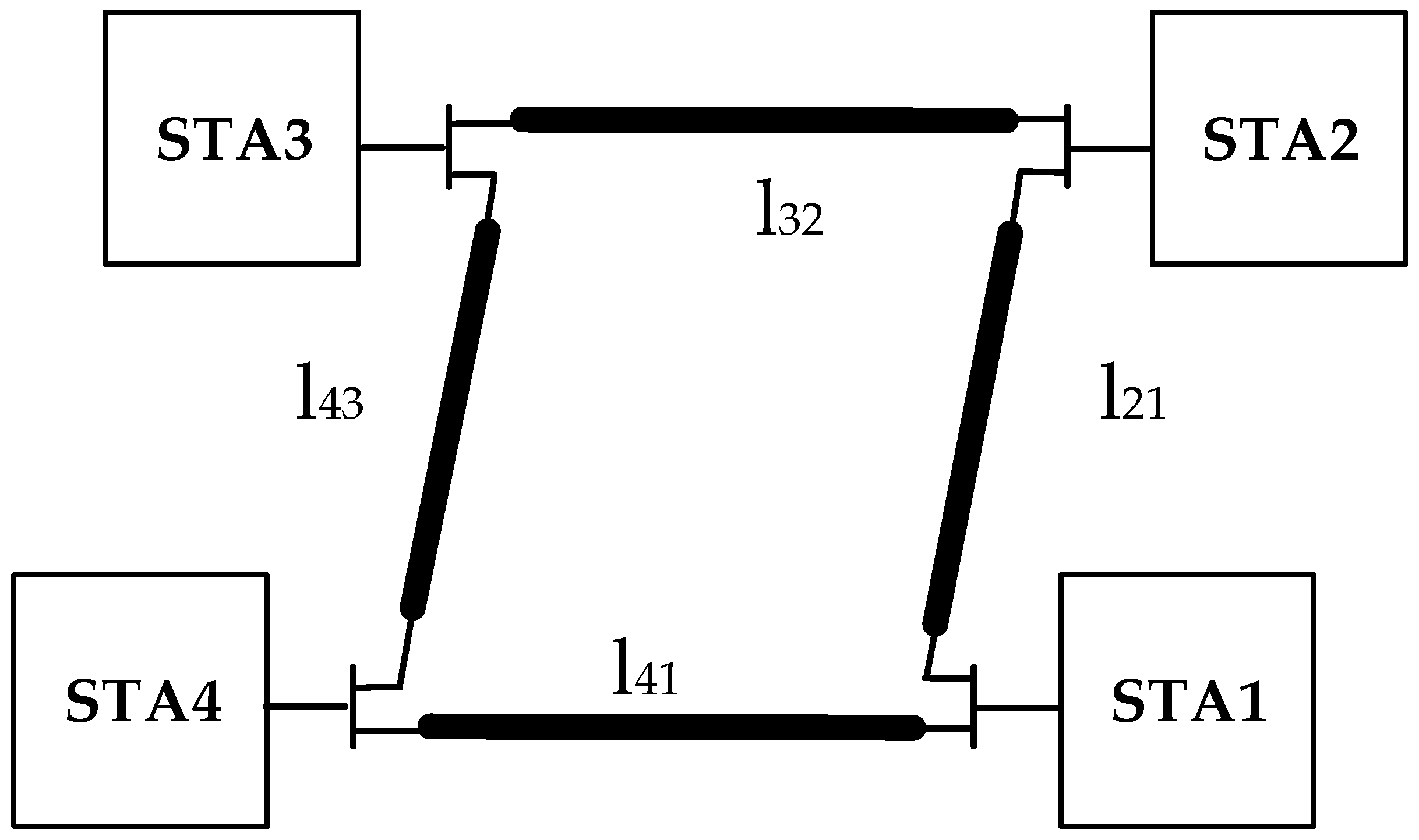
As an example, a MMC-HVDC grid with four converter stations is shown in Figure 8 and the power limit of each converter station and transmission line calculated by (5) is shown in

Table 1. Power limit of the example grid.

Stations and Lines	Power Limit (MW)
Station 1 (STA1) Ps1	1500
Station 2 (STA2) Ps2	750
Station 3 (STA3) Ps3	750
Station 4 (STA4) Ps4	1500
Lines (l21, l41, l32, l43) Pl	1500

. The power limit of each transmission line is equal.

If STA1 is the only receiving node and every device is working properly, the example grid will be a loop grid as shown in Figure 8.

First, the sending end grid and transmission section lines are determined. The transmission section lines include l₄₁ and l₂₁, and the sending end grid includes three nodes: STA2, STA3, and STA4, where STA2 and STA4 are sending node 1, and STA3 is sending node 2.

Then, the sending end grid is divided into two chains from sending node 2(STA3) according to (8). The two chains are STA3-STA2 and STA3-STA4, and each chain will get 375 MW from STA3.

Next, the maximum output power of each chain is calculated by (7). The results are 1125 MW (chain: STA3-STA2) and 1875 MW (chain: STA3-STA4).

Finally, the transmission capacity is calculated according to (11). The answer is 1500 MW. Similarly, if STA1 and STA2 are receiving nodes, the result will be 2250 MW.

If l₄₁ is broken and STA1 is the only receiving node, the example grid will be a single chain as shown in Figure 9.

First, the sending end grid and transmission section lines are determined. The transmission section line is l₂₁ and the sending end grid includes STA2, STA3, and STA4, where STA2 is sending node 1, STA3 is sending node 2, and STA4 is sending node 3.

Then, the maximum output power of this chain is calculated according to (7). The answer is 3000 MW.

Finally, the transmission capacity is calculated according to (6). The result is 1500 MW.

From the example, it can be seen that a loop grid can be divided into two independent sub-chain-grids and the calculation progress from (7) to (12) is demonstrated.

6. Discussions and Conclusions

This paper proposed a new calculation method of MMC-HVDC grid transmission capacity. First, the limit factors and grid basic topology is analyzed. Then, the limit factors and grid topology are simplified. On this basis, the transmission capacity calculation method of different basic topologies is proposed. Since every possible grid is made up of multiple basic topologies, the proposed method can be adapted to any MMC-HVDC grid. Furthermore, although the amount of calculation can be large at a complex grid, the calculation method can be easily realized by a program and has a great application prospect. Compared with the existing manual calculation method, which makes it almost impossible to finish the task, the proposed method has made great progress.

References

- Martinez-Rodrigo, F.; de Pablo, S.; Lucas, L.C.H.-D. Current control of a modular multilevel converter for HVDC applications. Renew. Energy 2015, 83, 318–331. [Google Scholar] [CrossRef]
- Zhang, J.; Zhao, C. Analysis and control of MMC-HVDC under unbalanced voltage conditions. Electr. Power Syst. Res. 2016, 140, 528–538. [Google Scholar] [CrossRef] [Green Version]
- Zhang, Y.; Ravishankar, J.; Fletcher, J.; Li, R.; Han, M. Review of modular multilevel converter based multi-terminal HVDC systems for offshore wind power transmission. Renew. Sustain. Energy Rev. 2016, 61, 572–586. [Google Scholar] [CrossRef]
- Tang, G.; Pang, H.; He, Z. R & D and Application of Advanced Power Transmission Technology in China. Proc. CSEE 2016, 36, 1760–1771. [Google Scholar] [CrossRef]
- Li, Y. The Fault Characteristics and Control Strategies of MMC Based HVDC Grid. Master’s Thesis, China Electric Power Research Institute, Beijing, China, 2017. [Google Scholar]
- Bu, G.; Li, Y.; Wang, S.; Zhao, B.; Wangm, T.; Yang, Y. Analysis of the short-circuit current of MMC-HVDC. Proc. CSEE 2017, 37, 6303–6312. [Google Scholar] [CrossRef]
- Du, X.; Guo, Q.; Wu, Y.; Pu, Y. Research on control system structure and coordination control strategy for Zhangbei demonstration project of MMC-HVDC grid. Power Syst. Prot. Control 2020, 48, 164–173. [Google Scholar] [CrossRef]
- Huang, D.; Yao, W.; Dong, N.; Xu, M.; Zhao, R. Study on comparison of transmission capacity and economy between UHV AC and EHV AC. Power Syst. Big Data 2018, 21, 45–52. [Google Scholar] [CrossRef]
- He, Q.; Zhang, B.; Ma, S.; Yi, J.; Zhang, J.; Jia, J. Research on measures increasing transmission capacity of Shandong section under UHV AC/DC access. Power Syst. Technol. 2018, 42, 126–132. [Google Scholar] [CrossRef]
- Moe, M.O.; Myint, T. Transmission capacity improvement using unified power flow controller with new control strategy. Int. J. Electr. Electron. Eng. Telecommun. 2021, 10, 225–232. [Google Scholar] [CrossRef]
- Teferra, D.M.; Ngoo, L. Improving the voltage quality and power transfer capability of transmission system using facts controller. Int. J. Energy Power Eng. 2021, 10, 10–19. [Google Scholar] [CrossRef]
- Ying, L.; Wu, L.; Man, X.; Zezhong, W. Study on steady-state operation region of VSC-HVDC converter station connecting new energy cluster by isolated network. North China Electric Power 2017, 8–13. [Google Scholar] [CrossRef]
- Qin, S.; Wang, S.; Zhao, B.; Sun, Y.; Yin, R.; Zhao, Y.; Yang, P. Study on safe and stable operation area for the converter station under scenarios of renewable energy generation sending through islanded MMC-HVDC. Power Syst. Technol. 2021, 45, 785–793. [Google Scholar] [CrossRef]
- Jiyun, L.; Dai, R.; Zhao, B.; Guo, W.; Zhao, X. Operation mode analysis of VSC-HVDC grid. Technol. Innov. Appl. 2021, 4, 141–142+146. [Google Scholar]
- Liu, C.; Wang, Q.; Chai, W.; Hu, Y.; Wei, Z.; Hu, S. Development and experimental research of ±535 kV hybrid DC circuit breaker prototype applied in Zhangbei four-terminal VSC-HVDC project. High Volt. Eng. 2020, 46, 3638–3646. [Google Scholar] [CrossRef]
- Xu, Z. VSC Based HVDC System, 2nd ed.; China Machine Press: Beijing, China, 2016; pp. 7–8. [Google Scholar]
Figure 1.
Diagram of MMC connected to the AC grid.