
A Proposed Framework for Identification of Indicators to Model High-Frequency Cities


1
Department of Land Surveying and Geo-Informatics, The Hong Kong Polytechnic University, Kowloon, Hong Kong, China
2
Smart Cities Research Institute, The Hong Kong Polytechnic University, Kowloon, Hong Kong, China
*
Author to whom correspondence should be addressed.
ISPRS Int. J. Geo-Inf. 2021, 10(5), 317; https://doi.org/10.3390/ijgi10050317
Submission received: 12 March 2021
/
Revised: 4 May 2021
/
Accepted: 6 May 2021
/
Published: 8 May 2021
(This article belongs to the Special Issue Geodata Science and Spatial Analysis in Urban Studies)
Abstract
:A city is a complex system that never sleeps; it constantly changes, and its internal mobility (people, vehicles, goods, information, etc.) continues to accelerate and intensify. These changes and mobility vary in terms of the attributes of the city, such as space, time and cultural affiliation, which characterise to some extent how the city functions. Traditional urban studies have successfully modelled the ‘low-frequency city’ and have provided solutions such as urban planning and highway design for long-term urban development. Nevertheless, the existing urban studies and theories are insufficient to model the dynamics of a city’s intense mobility and rapid changes, so they cannot tackle short-term urban problems such as traffic congestion, real-time transport scheduling and resource management. The advent of information and communication technology and big data presents opportunities to model cities with unprecedented resolution. Since 2018, a paradigm shift from modelling the ‘low-frequency city’ to the so-called ‘high-frequency city’ has been introduced, but hardly any research investigated methods to estimate a city’s frequency. This work aims to propose a framework for the identification and analysis of indicators to model and better understand the concept of a high-frequency city in a systematic manner. The methodology for this work was based on a content analysis-based review, taking into account specific criteria to ensure the selection of indicator sets that are consistent with the concept of the frequency of cities. Twenty-two indicators in five groups were selected as indicators for a high-frequency city, and a framework was proposed to assess frequency at both the intra-city and inter-city levels. This work would serve as a pilot study to further illuminate the ways that urban policy and operations can be adjusted to improve the quality of city life in the context of a smart city.
1. Introduction
A city is a complex system centred on people, resources and services. It includes residential buildings, industrial and commercial areas, schools, hospitals and other places and urban systems that interact with each other and become more vital because of human mobility. Ibn Khaldun (1332–1406), considered the founder of sociology, economics, historiography and demography [1], wrote in his best-known book, Muqaddimah or Prolegomena (‘Introduction’ in English), that cities resemble humans, in that they are born, grow, age, and die in an integrated life cycle. When political, economic, or other events occur during the city’s life cycle, the city must be restructured to restore its viability. Ibn Khaldun wrote that only cities that can be restructured will endure and flourish, and those whose functions cannot be restructured will die or perish. Undoubtedly, the perspective of Ibn Khaldun coincides with the proposal of Professor Michael Batty [2], a famous British urban planner and geographer, that
“In fact, the city is many times more complex than a single organism in that it is a collective of many pulses all firing at different rates but that are ultimately coordinated by our own human life cycles and rhythms. This we might think of as the ‘high-frequency city,’ in contrast to our traditional model of cities whose dynamics evolve and change over much longer time scales and at lower frequencies.”
Cities today are in a continuous state of growth and of successive responses to internal changes in the relationships among their various components and to the external influences imposed upon them. More than half of the world’s population lives in cities, and that proportion will increase to approximately 70% by the middle of the century [3]. Therefore, we should promote harmony with these changes and influences to allow cities to continue to thrive in the era of urbanisation by modelling the ‘high-frequency cities.’ The city represents a system of diverse functions, and the number and scope of such functions vary from city to city. From a short-term perspective, urban functions may change hourly because they support a variety of human activities 24 h a day [4]. An understanding of the dynamics of these functions would be beneficial to address current urban planning challenges, such as providing better public transit services, managing traffic congestion and making our cities smarter and more sustainable. Human activities play a significant role in the study of urban dynamics. For example, urban dynamics demonstrate human mobility and activities through time and space, as reflected in spatial interaction and changes in the urban structure over time [5,6].
In recent years, the main challenges in urban studies have been to understand human mobility and activities and their impact on urban dynamics and to infer urban functions at a high spatiotemporal resolution. Most studies in the field of urban planning and management have dealt with low-frequency cities, whose structure remains stable over years, decades and even centuries. Rapid urbanisation and the 24-h nature of most megacities have made today’s megacities more active, and urban mobility undergoes periodic and more frequent changes in the short term. Moreover, today’s megacities face various challenges in terms of short-term management and control. Traditional urban studies have successfully modelled the ‘low-frequency city’ and have provided solutions such as urban planning and road design for long-term urban development, such as the classical models of urban structures shown in Section 2. However, existing urban studies and theories are insufficient to model the dynamics of cities’ intense mobility and rapid changes and are thus unable to tackle short-term urban problems such as traffic congestion, real-time transport scheduling and resource management.
The dominance of computers and smartphones in most aspects of our daily lives and the emergence of the Internet of Things as an integral part of the fabric of the city itself have removed many obstacles to researchers’ and urban planners’ ability to plan and improve the city in the short term. Moreover, various types of flows, such as people, vehicles, freight, materials, goods, money and information, can be monitored at a high time resolution. These data have inspired us to change our thinking towards the high-frequency city. We note that the general idea of a high-frequency city was coined by Batty [2,7]. Although this idea was introduced more than two years ago, no explicit definition or indicators for modelling the frequency of a city have been established. In this article, we develop a framework for the estimation of a comprehensive index to assess the level of frequency at both intra-city and inter-city levels.
The remainder of this paper is organised as follows. Section 2 introduces the concept of a high-frequency city. Section 3 illustrates the methodology for selecting indicators that fit the concept of a high-frequency city and the proposed methodological framework for analysing the selected indicators to assess cities based on their frequencies. Section 4 then presents a set of 22 indicators selected for modelling the frequency of a city. Finally, Section 5 summarises this paper.
2. The Concept of a High-Frequency City
Since the early 20th century, urban planners and geographers have shown interest in the ‘nature of cities’, especially in terms of their growth in space and attraction to populations [8]. Researchers with an interest in urban studies thus began to propose models and answer questions about the urban structure. Ibn Khaldun pointed out in Muqaddimah that the first cities did not emerge suddenly and quickly but experienced several stages in their development. This pattern of development has also been observed over decades in the evolution of urban structures and its transition from monocentric to polycentric models; for example, the structure of Beijing city [9]. In the early 20th century, the conditions of transport and the urban environment made it possible for workers to afford accommodation near the city centre to reduce their daily transport costs. As a result, Burgess introduced the concentric zone model for a typical industrial city (e.g., Chicago) in 1925 [10], as shown in Figure 1A. In the 1930s, the cost of bus tickets became affordable for workers, and accessibility to the central business districts improved along transport routes [11]. In addition, some areas of cities became hubs for specific activities, and the growth and expansion of cities took the form of sectors based on socioeconomic groups. In 1939, Hoyt modified the concentric zone model to a sector model, as shown in Figure 1B, to describe the structure of cities. With the increasing number of car owners, the human movement has become more dynamic than ever and has allowed the specialisation of regional centres and the distribution of sources and services. Based on these developments, in 1945, Harris and Ullman proposed a multiple-nuclei model as the primary description of a polycentric city with a dominant central business district [11], as shown in Figure 1C.
However, these classical models are inadequate for today’s urban challenges because they are based on traditional types of data, do not account for the changes that occur in cities and are observed in the short term; thus, they only apply to what is called low-frequency cities. Cities are always in flux, and these dynamics are the pulse of the city. The dominant factor in these dynamics is the pattern of urban mobility. In addition, various political, social, religious and technical factors influence mobility and its frequency. An example of the impact of political decisions on free movement is the issue of the United Kingdom leaving the European Union (Brexit). This decision will inevitably affect the free movement of people, goods, services and capital between the United Kingdom and the European Union. The development of human-to-human communication technologies is changing lifestyles and mobility, as has happened with the advent of mobile phones and may continue to change in the future with the availability of satellite-based Internet and its complete coverage of the Earth. Because urban mobility patterns change frequently within a short time, we must change our thinking about cities from low-frequency to high-frequency models.
Today’s cities face many challenges and changing circumstances at a global level, including urbanisation, traffic congestion, air pollution, noise, multiculturalism and the emergence of slums in developing cities [13]. These challenges have led researchers and planners to address residents’ quality of life and meet their needs in two main orientations: smart cities and sustainable cities. The smart city is based on the use of information and communications technology in every subsystem of the city [14]. For a sustainable city, the focus is on preserving the existing resources and capacities of the environment and using these resources according to standards that do not deplete health or the environment [15]. Previous studies have developed a set of indicators or a composite index to assess transport performance and urban mobility to achieve the goals of different orientations of a city (e.g., smart city, sustainable city, competitive city and liveable city). Some of these previous studies are listed in Table 1. However, these orientations have shortcomings in the short-term analysis of a city, according to Batty [7]:
“Despite all the hype about the smart city and the generation of big data from networks of sensors that are likely to be installed everywhere, none of this has resolved the basic problem that faces us in our understanding of cities and the means we have to predict and design their future.”
As noted above, although the general idea of a high-frequency city was introduced more than two years ago, no explicit definition or indicators to measure the frequency of a city have been established. The first dilemma we faced was thus to propose a comprehensive and clear definition of a high-frequency city. A well-known example of ‘frequency’ in daily life is alternating current (AC), which periodically reverses direction (i.e., the electrons flow is bi-directional) and changes magnitude over time. From this point of view, a city can be considered as an AC circuit, with individuals, buses, taxis and information as electrons and origin/destination pairs as the north and south poles. Based on our vision related to the concept of a high-frequency city, we propose the following comprehensive definition:
“A high-frequency city is a self-organised city that can regain its pulse, balance its urban functions and continue to thrive and show resilience by creating an environment that is conducive for residents to engage in their various activities at various times while maintaining sustainability as much as possible, which can be observed, modelled and optimised via analysis of available geo-big data collected through the sensors and techniques inherent to smart cities with a fine spatiotemporal resolution.”
3. Methodology
This section is divided into two subsections: The first subsection presents the methodology used to create a literature database from which suitable indicators for the concept of the high-frequency city were extracted. The second subsection illustrates the proposed framework for the analysis of the selected indicators to assess the frequency of cities.
3.1. Review Methodology
A literature review was conducted in relation to mobility patterns and the concept of frequency, as well as the evaluation of smart and sustainable cities. The purpose of this study is to select indicators and propose a methodological framework for the analysis of these selected indicators in order to evaluate cities in accordance with the concept of frequency, as explained in Section 2. To select indicators that fit the concept of a high-frequency city, a content analysis-based review step was conducted, based on two basic phases: the construction of the literature database and the development of criteria for the selection of indicators. The literature review was used in the context of mobility patterns and transport network performance, as well as the review of the frequency concept and the assessment of mobility in a smart and sustainable city. The phase of the construction of the literature database is mainly based on the literature search strategy and study selection. It should be noted that the main database created consists of four sub-databases as follows:
- Database for Smart/Sustainability Assessment: This database has been constructed on methods, guidelines and procedures dealing with indicators for assessing mobility in smart and sustainable cities;
- Database for Exploring Human Mobility Pattern: This database has been constructed on robust existing methods and metrics used for human mobility and urban goods movement. Although there are indicators that cover the category of mobility in both approaches (i.e., sustainable and smart city), each indicator is examined from the specific concept of each orientation. For example, the goal of mobility indicators in the sustainable city reflects the extent to which the use of public transit systems is encouraged in order to maintain the sustainability of resources for future generations, even if it results in the city becoming inactive. This differs from our concept of the high-frequency city, where we look for indicators that reflect the extent of mobility and interaction of people within the city through time and space, as well as the monitoring frequency of these patterns within the city while respecting the principle of sustainability as much as possible;
- Database for Reviewing Metrics of the Selected Indicators: This database has been created to examine most existing metrics, methods and models for calculating the selected indicators, whether they are based on traditional methods or artificial intelligence methods such as machine learning or deep learning. Moreover, this database consists of literature related to the selected method in our proposed framework;
- Database for Understanding the Complexity of the City: This database has been created to understand the complexity of the city, as well as ways to represent this ever-changing complexity of dynamic systems in the city, such as the use of multilayer networks.
3.1.1. Literature Search Strategy
In order to create the literature databases, we first considered the relevant articles we were already aware of. Secondly, academic search engines, such as ‘Google Scholar’ and ‘Research Gate,’ were used. Search engine results were supplemented by reports from international and regional organisations and networks such as the Organisation for Economic Co-operation and Development (OECD), the World Business Council for Sustainable Development (WBCSD), International Association from Public Transport /UITP, Victoria Transport Policy Institute (VTPI), Institute for Environment and Sustainability, Joint Research Centre and CITYkeys in European Commission.
To construct the first database, the used keywords were ‘sustainable* mobility,’ ‘sustainable mobility indicator,*’ ‘sustainable city assessment,’ ‘sustainable city,’ ‘urban mobility indicator,*’ Index of sustainable urban mobility,’ ‘smart mobility,’ ‘smart mobility indicator,*’ ‘smart city assessment’ and ‘transport performance.’ In order to construct the second database, we used the following keywords: ‘mobility pattern,’ ‘travel pattern,’ ‘mobility behaviour,’ ‘travel behaviour,’ ‘human behaviour,’ ‘human movement,’ ‘goods movement pattern’ and ‘freight activity.’ As for creating the third database, we relied on some of the studies found in the previous database. We also collected additional research using keywords related to the selected indicators. To create the last database, the keywords used were ‘complex city,’ ‘city as systems,’ ‘self-organising cities’ and ‘multilayer network analysis.’ Furthermore, we checked the list of references in the selected articles and reports.
3.1.2. Studies Selection
The criteria developed for selecting appropriate articles and reports for our final literature database lists are as follows:
- Relevant: The purpose of the selected articles compatible with the purpose of the database in which it is to be included. For example, the articles and reports included in the first database provide a set of indicators to assess sustainability or smart city;
- External validity: The framework or methods of the article can be applied in various cities around the world;
- Expertise: The selected article is peer-reviewed, and the reports have been prepared by experts in reliable international organisations and international academic institutions.
In addition, the content of the selected article or report should relate in some way to the context of urban studies and mobility or be applied as much as possible to mobility assessment. Our final main literature database lists 336 documents, distributed as follows: 260 journal articles, 26 conference papers, 17 books and book chapters, 31 reports and 2 theses. The share of each sub-database of these documents is shown in Table 2.
We created a keywords co-occurrence network using VOSviewer 1.6.16 software. The keywords were created using the unique terms from the titles and abstracts of the included documents. We used the binary counting method for counting the number of occurrences for each term, and the minimum number of occurrences of a term was set to 5. Out of 8088 terms, 407 met the threshold. For each of the 407 terms, a relevance score was calculated. Based on this score, the most relevant terms were selected by selecting the 60% most relevant terms (default choice). In this way, the 244 most relevant terms are displayed in the density visualisation map (Figure 2). The density visualisation map of the co-occurrence of the 244 most relevant terms contained four clusters. The density of a term reflects the number of relevant keywords in the different documents where both were found. The distance between two terms gives an indication of the interdependence of the two terms.
3.1.3. Which Criteria, for Which Indicators?
Based on the intentions stated above regarding the consideration of a city as having greater complexity than a single organism and as having many impulses and expressing dynamic processes, attempts should be made to use big data and extensible open data to understand the frequency of the cities. Thus, several requirements have been suggested for the selection of efficient and applicable indicators for modelling high-frequency cities. In particular, these indicators should address key risk factors, should be compatible with the available data and should be sufficiently clear in the presentation to be used by all stakeholders. An extensive literature review was conducted based on the first and second sub-databases to identify indicators and metrics used in urban studies. To select the appropriate indicators, the following criteria were used, which were mentioned in various studies (e.g., [34,35]) and consistent with our study objective:
- Measurable with reasonable precision, depending on available data and high-frequency observations;
- Easy to understand and substantial;
- Benchmarkable (i.e., the indicator must reveal the performance of alternatives);
- Scalable (i.e., the indicator must be suitable for different spatiotemporal resolutions);
- Specific (i.e., the indicator must evaluate the exact mobility aspects).
3.2. Proposed Framework for Modelling High-Frequency Cities
This subsection discusses our proposed framework, including the development of a mechanism to compare and analyse high-frequency cities. This has particular relevance because no study has attempted to identify indicators to evaluate a city’s frequency. A methodological approach must therefore be proposed to identify indicators to evaluate high-frequency cities. As demonstrated in Figure 3, our proposed framework consists of two phases: pre-processing and high-frequency city analysis.
3.2.1. Pre-Processing
This phase includes defining the indicators based on the available data sources and pre-processing the data sources.
Defining the Indicators
To determine a city’s frequency, it is imperative to consider indicators that include different analytical dimensions, such as the environmental, socio-economic and mobility dimensions. Although most of the indicators reflecting the frequency of cities are associated with mobility, they are somehow linked to environmental and socio-economic dimensions. Each indicator has an economic or social benefit to the individual or to society as a whole. The indicators related to mobility are relevant in the context of daily human travel behaviour. The selection of indicators depends on a review of the literature in urban research and the quality of their fit with the concept of a high-frequency city in this study. After reviewing numerous journal articles and reports from organisations and departments involved in urban studies, the most suitable indicators compatible with mobility big data were selected. In this study, we classified the indicators into five categories, namely human mobility, public transit systems (PTSs), road network (i.e., vehicular movement), urban goods movement (UGM) and land use.
This study aims to model high-frequency cities by analysing the changes that occur over short periods of time; therefore, its focus is on the selection of short-term and semi-short-term indicators, the use of which can reduce the dependence on long-term indicators for monitoring changes. Short-term indicators are those for which changes in values can be observed within seconds, minutes, hours, days or weeks, semi-short-term indicators are those for which changes in values can be observed over a longer time (i.e., months), whilst long-term indicators embrace changes over years and decades.
Pre-Processing Data Sources
As the amount and variety of data increase, the associated uncertainty also leads to mistrust in the resulting analysis process and the decisions made. As can be seen from the proposed framework, we rely on a diversity of sources and a variety of data, so there must be a pre-processing phase aimed at identifying uncertainties and trying to mitigate them. In big data analytics, artificial intelligence approaches offer more reliable, faster, and more scalable findings than traditional data techniques and platforms [36]. In the previous literature, there are many theories and techniques for dealing with uncertainty, and the most common approaches are discussed in these studies [36,37]. Figure 4 shows the common approaches used for measuring the uncertainty in big data.
To process big data accurately and with certainty of results, mitigating the uncertainty inherent in such data must be at the forefront of any technique that is to be applied. Hariri et al. summarised the strategies used for uncertainty mitigation (ibid), as shown in Figure 5.
3.2.2. High-Frequency City Analysis
The second part includes analysis steps for future empirical analysis. As seen from the methodological framework, this analysis can be carried out on both the intra-city and inter-city levels. To assess a city’s frequency at both levels, three main steps are implemented: addressing aggregation strategies, indicator analysis and assessment and ranking of alternatives (i.e., spatial units or cities). The following subsections illustrate in detail the steps of our proposed framework.
Addressing Aggregation Strategies
Given our dependence on diverse source data, as well as the possibility of applying the proposed framework at intra-city and the inter-city level, we need to address the Modifiable Areal Unit Problem (MAUP) and the Modifiable Temporal Unit Problem (MTUP) (e.g., spatial and temporal aggregation). As can be seen from the proposed framework, both MAUP and MTUP effects should be addressed at the intra-city level, but only MTUP effects should be addressed at the inter-city level. This is because MAUP effects arise when aggregating the available data into different spatial units. The spatial units used for the intra-city level can be represented by grid cells, traffic analysis zones and spaces between road networks (i.e., street blocks). For more details about MAUP and MTUP, refer to [38].
Indicator Analysis
In our proposed framework, the indicators can be analysed at both the inter-city and the intra-city level, and the analyses at both levels involve the same steps. As shown by the proposed framework, the indicator analysis phase consists of two parallel boxes, namely the white box and the black box. The white box refers to the traditional data analysis techniques and applications of network theory. Scholars in urban research and transport geography have particular incentives to represent urban spatial interactions as real networks, especially the flows of people and vehicles. Most urban network analyses rely on methods developed for social networks. Although most studies of urban networks have used traditional centrality measures to analyse the networks using only topological attributes, Senousi et al. considered both topological and geometric attributes to analyse public transit networks (PTNs) using smart card data (SCD) [39]. Moreover, most urban systems do not operate in isolation, so it is advisable to use multilayer networks whenever possible in the analysis of indicators that consider topological and geometric attributes. Škrlj et al. presented an overview of the tools and software used for analysis and visualisation of single-layer and multilayer networks [40]. The black box refers to artificial intelligence techniques, such as deep learning. Deep Learning is an innovative methodology for making inferences on massive or complex data. The development of deep learning provides a black box to depict geospatial patterns. Various techniques were applied in urban studies, such as classical neural networks, convolution neural networks (CNNs) and graph neural networks (GNNs). With the advent of graph neural networks, an effective method for dealing with graph-structured data is available [41]. This technique is a promising avenue for future urban studies, as there are many important real worlds in the form of networks or graphs.
City Assessment and Ranking
The final phase in the indicator analysis comprises three steps: determining the weights for the indicators, ranking the alternatives, and calculating the composite index for the high-frequency city (i.e., High-Frequency City Index (HFCI)). The alternatives are represented at the intra-city level by spatial units, whilst at the inter-city level, they are represented by cities. First, the weights of the indicators can be calculated with the entropy weight method (EWM), a common technique used for weighting in multiple-criteria decision-making that works with both quantitative and qualitative data. Unlike subjective fixed-weighting methods, such as the Analytic Hierarchy Process (AHP) and the Delphi method that were used in previous studies related to sustainability city, EWM avoids the influence of human bias on the weights of indicators, which reduces human error and leads to results more consistent with the facts, thus increasing the objectivity with which a composite indicator is created. In this paper, the EWM is used to estimate the weights of the indicators as follows.
In the EWM, assuming that the number of indicators is and the number of alternatives is ; the estimated value of the indicator in the spatial unit is denoted as . The first step in this method is to normalise the indicator values to an appropriate scale. The normalised value of the indicator in the spatial unit is defined as and can be calculated with the following formula [42]:
After normalising the indicators’ values, the matrix of normalised indicators is . Using this method, the entropy of the indicator can be calculated as follows (ibid):
The value in Equation (2) can be estimated by Equation (3):
where is the number of spatial units. The entropy weight of the indicator is then estimated by the following formula (ibid):
The lower the entropy value , the higher the entropy weight of the indicator, and the greater the effect of the indicator (and vice versa).
Second, the Technique for Order Performance by Similarity to Ideal Solution (TOPSIS method) is the most common and direct method of multiple-criteria decision-making. The TOPSIS method is used when determining the preference order of alternatives, making it an ideal choice for ranking spatial units or cities. The basic principle of this method is to identify both sides—positive and negative—of the ideal solution. In other words, the alternatives are ranked according to two criteria: the shortest distance to the positive ideal solution and the longest distance to the negative ideal solution. The intent of identifying a positive ideal solution is to maximise the indicators that lead to benefits and minimise those that lead to costs (and vice versa for identifying a negative ideal solution) [42]. The TOPSIS method is applied in this study because it is simple, it facilitates the calculation process, it can accommodate a large number of alternatives, and it considers the distance between the two sides of the ideal solution.
This method includes eight steps: (1) building the indicators’ value matrix, (2) normalising the indicators’ values, (3) determining the indicators’ weights, (4) constructing the matrix of the normalised value of the weight, (5) identifying the positive and negative ideal solution, (6) computing the distance between each alternative and each side of the ideal solution, (7) computing the relative proximity to an ideal solution and (8) ranking the alternatives. The first three steps in this method are performed in the previous part by applying the EWM. The remaining steps in the TOPSIS method are therefore dependent on values previously calculated with the EWM. The fourth step can then be performed to compute the normalised value of the weight by multiplying the indicator’s weight by a normalised value , as demonstrated in the next equation:
The ideal solution can then be identified. Here, the positive ideal solution consists of the best value of each indicator from the normalised weighted matrix , and the negative ideal solution consists of the worst value based on the normalised weighted matrix. Equations (6) and (7) illustrate how to calculate and .
where and express the benefit and cost indicators, respectively. The best and worst values of the indicator are represented by and , respectively. The greater the benefit indicator, or the lower the cost indicator, the more favourable the evaluation results (and vice versa). The Euclidean distance can be used to compute the separation distance between each alternative and the positive ideal solution as follows:
The separation distance between the alternative and the negative ideal solution can be estimated with the following formula:
The relative proximity to the ideal solution can then be estimated as in Equation (10).
The resulting values output by Equation (10) are restricted to the unit interval, , where the larger the value of , the better the alternative. A set of alternatives can then be ranked based on the descending order of .
Third, our proposed index (HFCI) can be used to provide a comprehensive value representing the frequency of the city based on a set of selected indicators. HFCI can be estimated using the following formula:
where is the score of frequency of spatial unit; is the normalised value of the indicator in the spatial unit; and express the benefit and cost indicators, respectively.
After the indicator analysis is implemented, the results of the indicator analysis of future empirical analysis can be considered and appropriate actions to enhance urban planning can be recommended.
4. Results: Indicators of High-Frequency City
A content analysis-based review was conducted to identify indicators and metrics used in urban studies. After reviewing the journal articles and reports in the first two databases created, a set of indicators was selected using the above criteria. The proposed set of indicators is divided into five domains or categories: human mobility, PTSs, road network, UGM and land use. The proposed indicators are relevant to these five categories, and most are generally related to urban mobility in some way. Figure 6 shows the 22 indicators used to analyse the frequency of the city in a hierarchical structure divided into the five categories listed above, and the type of frequency of each indicator is illustrated in terms of its temporal dimension (i.e., short-term or semi-short-term).
4.1. Proposed Indicators for High-Frequency Cities
In this subsection, we review the 22 indicators selected for the screening of high-frequency cities and provide examples of how these widespread metrics are used to estimate the indicators in the literature. It must be noted that the list of metrics used to estimate each indicator presented in this article is not exhaustive.
4.1.1. Human Mobility
This category presents the proposed indicators with relevance to human mobility. This category includes only short-term indicators.
Incoming/Outgoing Flows
As illustrated in Section 2, in which the concept of the high-frequency city was discussed, we liken the flow of vehicles, people, money and even information to the movement of electrons in an AC circuit due to our belief that these changing flows in both directions are the lifeblood of cities. In recent years, with the extensive integration of information and communications technology in cities, many systems have been established to monitor activity in cities at a very fine temporal resolution. Various technologies have also been introduced to track human mobility, such as smart cards and global positioning devices placed in various vehicles to provide information about passengers or traffic flow at a fine spatiotemporal resolution. The flow of passengers over space and time is affected by workdays, holidays, cultural events, residential areas, central business districts, workplaces and other factors such as climate events [43].
A considerable number of studies have attempted to estimate and predict passenger flow. Yu et al. examined the 24-h fluctuations of the daily average passenger flow and the intensity of passenger flow of metro lines [43]. They proposed a peak hour coefficient to determine the degree of crowding of passenger flow at a particular time. With the broad application of complex network theory in urban transport networks, several researchers have created passenger flow networks and then analysed their structural properties, such as flow weight distribution and node throughflow distribution. The relationship between network centrality and passenger flow has been investigated in various articles (e.g., [39]). In this sense, we can create a passenger flow multilayer network and analyse the centrality distribution and community structure.
Density Changes
People are most mobile in cities, which leads to changes in the population density in space. Hence, tracking population density allows us to explore the extent to which the frequency of the city is changing. In recent years, population density has been estimated using remote sensing technology or traditional data (e.g., population count data from censuses). However, the estimation of population density changes based on traditional datasets has deficiencies in spatiotemporal resolution relative to mobile phone data. Mobile phone data provide the ability to track population density changes at a high spatial resolution over various time scales of hours, days, weeks, months or even from year to year. Deville et al. examined population density dynamics using call detail record data [44].
Travel Distance
Travel distance is a fundamental factor in modelling human mobility over a given time. The distance calculation is usually based on data sources. In recent years, an increasing number of studies of human mobility have used travel time and travel distance measures to identify the human mobility patterns within a city. Of these measures, the flight length, jump length and displacement are worthy of mention [45]. It should be remembered that mobility occurs over a wide range of distances, and as the distance varies, the apparent speed and the means of transport vary [45]. Furthermore, Shi et al. demonstrated that younger adults travel longer distances than older adults [46]. This reaffirms the value of a travel distance indicator for evaluation of high-frequency cities because longer distances travelled by residents are an obvious indication that most of the population is of young adult age. Globally, young people are essential human resources for the development and revitalisation of cities. Therefore, a city whose residents travel long distances is the most liveable and energetic.
Radius of Gyration
In physics, the radius of gyration () is equivalent to the mass moment of inertia, but researchers in human mobility have used this metric to characterise an individual’s distance from the centre of mass of his or her trajectory [47]. We can compute the radius of gyration for each spatial unit or city for a given period and study the variation in the values over time. The general formula for is as follows:
where is the radius of gyration for a given spatial unit (); is the number of origins and destinations of spatial units to and from a given spatial unit; is the total number of spatial units; are the coordinates for the destinations and origins; is the centre of mass.
Distance between Mean Centres (DMC)
The mean centre is the average point, and the coordinates of this point can be calculated from the average of the x- and y-coordinates for certain features. Although few studies in human mobility have used this metric, it is a core part of our proposed indicator (i.e., DMC) because it demonstrates the degree of interaction of a given spatial unit with the remaining spatial units within the city. First, the ingoing mean centre coordinates (, ) can be computed with Equation (13), where and are the coordinates of the centre of the spatial units that inbound to a given spatial unit (). Second, the outgoing mean centre coordinates (, ) can be computed with Equation (14), where and are the coordinates of the centre of the spatial units that outbound from a given spatial unit (). Finally, the Euclidean distance can be applied to compute the separation distance between the ingoing and outgoing mean centres (), as illustrated in Equation (15). The greater the number of different spatial units that interact with a given spatial unit, the greater the distance.
4.1.2. Public Transit Systems
PTN Coverage
Public transit (PT) is the portion of the transport modal split. PT is considered accessible to a wider range of commuters than private transport and, unlike private transport, is managed by public authorities or transport operators. It is possible to improve mass mobility and urban quality of life by establishing PTNs within walking distance of most people. Urbanisation and urban growth have contributed to an increase in the demand for mobility. When PTN coverage is insufficient to meet demand, waiting times increase, and delays and congestion occur on PTSs and roads [13].
PTN coverage is one of the underpinnings to quantify PT accessibility and is well known to transport planners as an important indicator of PT service performance. PTN coverage has been used in various research papers (e.g., [21]) as an indicator related to the mobility category for a smart, sustainable and competitive city. Dodson et al. calculated the spatial coverage of PT services based on population location [48], and they computed the PT service coverage with consideration of the temporal dimension (e.g., morning peak, inter-peak, evening peak, off-peak).
Transport System Diversity
Because cities have more economic opportunities than rural regions, urban population growth has increased significantly around the world but without the same level of development in urban transport infrastructure. While the transport needs of various classes of urban dwellers are changing, the choice of transport options is not sufficiently diverse in most cities. Litman argued that the diversity of the community and the need to meet diverse transport demands require that the transport system also be diverse [49]. The diversity of a transport system lies in providing diverse choices in transport mobility and accessibility on a 24-h basis by providing different types of transport modes and services.
A transport system’s diversity can be calculated with various metrics, such as the quality and quantity of travel options, the modal split, the quality of non-motorised transport and the amount of non-motorised transport [23,31,32,33,35]. The most common metric to reflect the diversity of a transport system is the modal split (i.e., modal share), which is determined by computing the share of trips by each mode and using Shannon entropy, such as in [15].
Intermodal Connectivity
PTSs usually comprise various modes, and daily commuter trips may include a transfer within the same mode or across modes. Intermodal connectivity gives commuters the opportunity to use a combination of transport modes [35]. Therefore, to reduce congestion, it is necessary to plan for inter-city and intra-city PT to discourage the use of private vehicles. Intermodal connectivity not only enables connectivity among mobility subsystems and facilitates transfer for commuters, but it also improves cities’ vibrancy and liveability by providing individuals with numerous transport options. For example, a limitation in connectivity may lead some commuters to stop using PT services [50].
The intermodal connectivity indicator examines the extent of transfer among mobility subsystems (i.e., the availability of intermodal transfer). The authors of one study [51] considered the temporal dimension to quantify intermodal connectivity at high-speed rail stations. They introduced three metrics to quantify connectivity: intermodal time, intermodal integral time and intermodal entropy. The intermodal time indicates the time required to reach a specified mode from other modes, and the intermodal integral time expresses the sum of the intermodal time for all available modes, and the intermodal entropy expresses the degree to which various modes are unbalanced. Moreover, De Stasio et al. modified the interconnectivity ratio metric by considering the transfer time, which includes boarding, alighting and waiting times [52]. They also presented degree centrality and closeness centrality as metrics to reflect the network’s connectivity. A multilayer network can be used to estimate the centrality measurements as metrics for quantifying the connectivity of PTSs.
PT Reliability
Travel time takes on increasing importance as economic growth continues. The commuters’ waiting time at PT stops is generally the largest share of the total time cost of a trip, for which the passengers’ waiting time can sometimes be double the in-vehicle time [53]. PT reliability reflects the extent to which the transit vehicles adhere to announced schedules, and the headway between vehicles on the same line remains constant (i.e., headway regularity). From the operators’ point of view, greater reliability leads to lower operating costs and higher revenue, as the likelihood of attracting and retaining additional commuters increases [54]. The primary cause of poor reliability is headway irregularity, which also results in longer waiting times and unequal distribution of commuters among vehicles.
Kathuria et al. presented a methodical review of PT reliability measures [55]. They categorised the reliability measures into a four-quadrant approach as follows: (1) reliability measures based on the waiting time, (2) reliability measures based on the headway regularity, (3) reliability measures based on the travel time and (4) reliability measures based on the transfer time. The metrics for the PT reliability indicators in this article are those relevant to headway and waiting time.
Resilience to Disaster
The resilience of a PTN indicator is one of its most significant properties because it reflects the ability of cities in general, and their transport networks in particular, to reorganise themselves to meet the public’s transport needs to the maximum extent possible and to restore near-normal system functionality following a disaster. Previous studies conducted a literature review on measures of PTN resilience from several perspectives [56,57]: (1) resilience to severe weather events, (2) resilience to long-term climate change, (3) static resilience, (4) dynamic resilience (cascade failure-based resilience) of single-layer PTNs and (5) dynamic resilience of multilayer PTNs. The first and second perspectives examine the impact of climate on PTN performance and resilience. Examination of resilience from the third, fourth and fifth perspectives has been considered in the wake of terrorist and cyber-attacks on PT stations and services, such as the London transport network bombings during the morning rush hour in 2005 and the cyber-attacks in Ukraine in 2015, which caused the failure of power plant control servers and led to power outages for some transport network services.
Service reliability, which includes indices such as headway reliability [58] and travel time uncertainty [59], has been used as an indicator of resilience in many studies. In our view, travel time and headway are inappropriate metrics to calculate the resilience of PTNs to extreme events such as natural disasters or terrorist and cyber-attacks because they do not consider the networks’ topological structure. Many studies have investigated the static and dynamic resilience of single-layer networks (e.g., [60,61]), and others have investigated those of multilayer networks (e.g., [62,63]). The indicator most commonly used to measure resilience is the relative size of the maximum connectivity cluster and the average shortest path length, which are derived from complex network theory metrics.
Occupancy Rate
The changing demand for PT services throughout the day, week or year has motivated PT operators to make decisions to adjust to such fluctuations in demand. One such decision has been to implement more rational scheduling for transport services; this policy encourages PT operators to continuously update the frequency of services to optimise the balance between transport supply and passenger demand [64], which is achieved by determining the occupancy rates of PT vehicles. The occupancy rate refers to the quotient of the PTN’s real performance per period and per direction and the maximum capacity [57]—in other words, the proportion of the maximum active vehicle capacity occupied at a given time.
The purpose of this indicator is to calculate the average load factor for all means of urban transport. Although this indicator has been mentioned in the evaluation of sustainable cities (e.g., [24,27,35]), it can also be used to evaluate high-frequency cities because it reflects the variability over time in the number of people per operating vehicle. Several organisations use this indicator, including the European Environment Agency, the United States Department of Transportation, the World Bank and the Public-Private Infrastructure Advisory Facility. The first two organisations proposed the load factor metric, although the first limited its use to freight only and then discontinued this metric in 2017 [65,66]. The last two organisations proposed the passengers per vehicle per day metric, which can be estimated by the total number of passengers transported over a specified time, divided by the total number of active vehicles over the same period and divided again by the number of days during the period [67].
Active Vehicles
This indicator corresponds to the occupancy rate indicator but is intended to calculate the total number of vehicles that make at least one trip during a specific day [68]. It reflects the daily activity of vehicles within the city. This indicator can be applied alone or embedded with the passengers per vehicle per day metric as a sub-indicator that follows the occupancy rate indicator.
4.1.3. Road Network
Traffic Flow
Traffic flow expresses the number of vehicles that pass over certain points or segments per unit of time. Traffic flow data have been collected in recent years using diverse traffic sensing devices, the most common of which are traffic surveillance cameras, radio frequency identification detectors and loop detectors. However, most of these sensing devices have a deficient spatiotemporal resolution because they are placed at specific points and are sparsely distributed throughout the road network. The advent of position sensors such as global positioning systems in smartphones and in vehicles has allowed the collection of massive amounts of traffic flow data. With the rapid development of artificial intelligence algorithms, various deep learning methods have been used to predict traffic flow at a fine spatiotemporal resolution. Wang et al. estimated the traffic flow in large road networks by integrating the licence plate recognition data and the taxi GPS trajectory data [69]. With the broad application of complex network theory in the urban transportation network, Liu et al. created a taxi flow network and analysed the structure of the city based on the created network [70].
Travel Time Uncertainty
Users and operators of PTSs appreciate travel time and its uncertainty because they are core indicators of service performance. To facilitate real-time management, operators of PTs require reliable estimates of travel time [71] and the variability of travel time. In an investigation of travel time, Bates et al. claimed that in most cases, a decrease in variability is more likely to be appreciated by commuters than a decrease in the average travel time required for daily trips [72]. A decrease in variability reduces commuters’ discomfort and stress as a result of confusion over departure times and route choices.
Travel time variability takes various forms, including vehicle-to-vehicle, period-to-period and day-to-day variability, among which day-to-day variability is the most commonly studied [71]. Numerous metrics have been used in recent years to estimate variability in travel time. In 2006, the United States Federal Highway Administration proposed four reliability measures, namely [73] the 95th or other percentile travel time, the buffer index, the planning time index and the frequency of congestion. The coefficient of variation is the most popular metric in transport studies, in which it is used to quantify accessibility when considering travel time uncertainty [74].
Traffic Congestion
Whilst transport has contributed enormously to the social, economic and political growth of cities, it also leads to adverse consequences such as congestion, delays and accidents. In several cities around the world, the problems of traffic congestion and delays have reached unprecedented levels and have become major impediments to the free flow of traffic. These problems have arisen from the ineffective use of road space and the increasing number of vehicles on the road network due to the demand for human mobility [75]. Researchers and transport experts have proposed various metrics and techniques for accurate estimation of traffic congestion; however, no single metric has been universally accepted for the calculation of traffic congestion in cities or on roads. Various metrics are implemented in various countries and even at the provincial level within an individual country [76]. Afrin and Yodo classified the congestion metrics into six classes based on the benchmarks used to develop them [76], as shown in Figure 7.
Road Safety
Rapid urbanisation and the increase in the number of motor vehicles worldwide have led to an increase in traffic collisions, resulting in deaths and serious injuries. According to the World Health Organization (WHO)’s ‘Global status report of road safety 2018,’ more than 1.3 million traffic fatalities occur worldwide each year. In addition, the WHO highlighted that each year, approximately 12 million people worldwide suffer road traffic injuries [77]. Although road safety does not reflect the level of mobility as directly as other indicators, it exerts an indirect effect on human mobility and increases the quality of life in the city. Unfortunately, traffic accidents result in road traffic interruptions, which create gridlock on the road network. Furthermore, traffic accidents are among the major causes of death worldwide among people between 15 and 29 years of age [77]. This age group is more dynamic and active and has a direct impact on both inter-city and intra-city mobility function. Young adults, therefore, make cities more vibrant and flexible for redevelopment.
In recent decades, researchers and policy-makers have developed metrics to evaluate road safety performance, including the mortality rate, which is given as fatalities per 100,000 population, fatalities per billion vehicle-kilometres and fatalities per 10,000 registered vehicles. Al-Haji proposed the road safety development index [78], which refers to the level of road safety in a particular country and can be used to compare countries at a specific time.
4.1.4. Urban Goods Movement
The UGM expresses the movement of goods or things rather than persons. According to Woudsma [79], UGM results from the reciprocal relationship between ‘elements’ and ‘actors,’ in which the elements represent the physical aspects of the transport system and the actors represent the people or organisations that make decisions regarding the movement of goods, as illustrated in Figure 8. It should be noted that the movement of goods is necessary for various activities in the urban environment, both economic and social. Few studies have examined the dynamics of UGM patterns and how they differ from human mobility and traffic flow patterns. The indicators used in the study of UGMs follow the same concepts as those in human mobility. This section reviews the three most common indicators in the literature related to UGM.
Freight Traffic Volume
This indicator reflects the number of freight vehicles (e.g., trucks or vans) on the road and is given as the number of trips or online orders in a specified period. The consumption of goods depends on the density of the urban population; the greater the density of the population and the more vibrant and energetic a city is, the greater the demand for goods. This leads to more frequent movement of goods, which automatically affects the dynamics of UGM patterns. This indicator has been used in most previous studies (e.g., [80]).
Vehicle-Kilometres Travelled
This indicator can be estimated by summing the kilometres travelled by all trucks within a particular period. This indicator is also known as displacement, and it is used in some studies to determine the pattern of UGM (e.g., [81]).
Network Properties
Several network properties can be used to explore the dynamic properties of UGM after translation of the commodity movement characteristics into a network, especially graph density, number of nodes, number of edges, average degree and average strength [81]. This indicator is suitable for use in analyses at the inter-city level.
4.1.5. Land Use
All indicators in this category depend on data that can be observed in the semi-short-term.
Transport Land Consumption
The transport sector manages human mobility and the transport of goods and supplies the transport infrastructure. The volume of transport depends on the supply of transport (e.g., transport infrastructure) and the demand for transport. Therefore, the land dedicated to transport infrastructure, which includes both direct use (e.g., motorways and railways) and indirect use (e.g., car parks), is a key factor in the generation of transport activity in terms of the infrastructure induced by human mobility [82]. This notion is in line with the view of Ashby, who introduced the concept of ‘self-organisation’ in 1947, stating that each subsystem can adapt to the conditions formed by the remaining subsystems.
Various metrics have been used in urban studies to represent transport land consumption (e.g., [13,82]). The most straightforward metric is the surface area devoted to transport infrastructure. This metric shows the extent of the decision-makers’ interest in transport infrastructure, which facilitates human movement and affects transport conditions. This metric should be scaled when used to compare cities or spatial units. Values can be scaled in various ways, including calculation of the per capita land area dedicated to transport or the ratio of land area dedicated to transport to the total land area used for public infrastructure [21]. Some studies have also used the length of the transport network, which is also scaled by dividing it by the area, resulting in a so-called ‘network density’ [82], or by dividing it by the population density, resulting in a so-called ‘network length per capita.’ Some studies have considered the time dimension, reflecting the actual area of infrastructure used multiplied by the actual time of use [83].
Land-Use Mix (LUM)
Land use and transport form our cities. Land use refers to the ways that individuals use land and resources for certain purposes, such as for residential purposes, commercial activities and recreation. The relationship between land use and the transport system is essentially reciprocal (i.e., it has a cyclical nature), as shown in Figure 9. Land use is a catalyst for human mobility and activities. Accordingly, an increase in the intensity of land use generally increases transport demand in terms of facilities and infrastructure investment, thereby improving accessibility [84]. This improved accessibility is a catalyst for increasing land values and land development and thus trip generation. This cycle of reciprocity is thus repeated because once land-use activities increase, the demand for transport increases [85]. Mixed land use, which typically involves a synthesis of residential, recreational and commercial activities, is considered to strengthen urban vitality and offer several socio-economic benefits [86].
LUM indicator has been used in several studies to explain urban vitality, walkability, sustainability and transport planning [15,82,87]. Several studies of transport have reported that multifunctional land use has a positive correlation with the frequency of non-motorised trips and a negative correlation with the frequency of motorised trips (e.g., [88]). Song et al. provided a systematic overview of the mathematical formulae and conceptual foundations of the prevailing methods of LUM [89] in which they categorised the methods into four groups: the Percentage and Exposure Index; all varieties of the Atkinson Index; the Balance, Entropy and Herfindahl–Hirschman indices; and the Dissimilarity and Gini indices. The most applicable is the entropy method because it allows consideration of more land-use classes. The entropy formula is as follows:
where is the score of the land-use mix; is the percentage of land use in the region; is the number of land-use classes. The value of ranges from 1 to 0; a value of 1 reflects the maximum potential mix, and a value of 0 indicates that the region is monofunctional.
Due to technological advancements and the availability of mobility big data, such as mobile phone data and point-of-interest data, several researchers have used such data to reveal the land-use mix at a fine spatiotemporal resolution (e.g., [4]).
Vitality
With the global growth of cities since the 20th century, major cities have experienced flourishing economies and cultural expansion. However, this unprecedented urbanisation has led to many problems in major cities, including urban sprawl, housing vacancies and the imbalance of urban functions [90]. These problems pose a challenge to the development of the ‘high-frequency city’ theory as the diversity of the urban fabric decreases and urban vitality deteriorates. To optimise the urban fabric, it is vital to determine urban vitality in large cities. The principle of urban vitality is inseparable from the intensity of human activities in public spaces [91], so urban vitality has also been used to establish planning principles to strike an equilibrium between human activity and the built environment. In general, the two most common models used to quantify the built environment are three-dimensional and five-dimensional, as shown in Figure 10. More details about the dimensions embedded in these models can be found in the literature [92].
The numerous published studies on the estimation of vitality have applied various perspectives and data sources. Jacobs defined urban vitality as street life on a 24-h basis [86]. Lynch argued that a vital city is one that effectively addresses the needs of its residents within a safe environment [93]. Braun and Malizia proposed the Urban Form Index to reflect neighbourhood vitality based on five variables: Inter-circulation systems, External traffic systems, Density, Land-use mix and Accessibility [94]. Yue and Zhu investigated the relationship between vitality and street network centrality in both walking and driving modes [95]. They indicated that street network centrality (e.g., closeness, straightness and betweenness) has a significant influence on urban vitality. In this sense, and with our belief that transport systems do not function separately, we can adopt the concept of multilayer networks for the estimation of the vitality indicator.
4.2. Impact of COVID-19 and Driverless Mobility on the Frequency of the City
In mid-March 2020, the World Health Organization (WHO) declared COVID -19 a global pandemic in light of the rapid spread of the epidemic across states and countries. The epidemic continues to have many negative and catastrophic effects on social and economic aspects in various sectors, including travel and mobility, making it the first global health disruption with immediate and devastating implications on various sectors at this scale in 100 years [96]. Given that transport systems play an essential role in controlling or spreading the epidemic because they serve in some ways as vectors for the transmission of infectious diseases between different places, some governments have taken seriously the guidance from WHO to adopt isolationist policies by reducing the mobility of transport systems. Many countries have imposed lockdowns as well as states of emergency, banning unnecessary movement and restricting participation in various activities, imposing restrictions on social distancing to maintain public health and contain the spread of coronavirus [97]. In addition, many governments, such as Hong Kong, have passed resolutions and decrees eliminating the need for daily travel, such as closing recreational facilities and stores that do not sell food and medicine and banning public gatherings. To meet the needs of isolation, many universities, schools and companies have switched to virtual environments for learning and working remotely. Some people also impose self-restrictions by limiting their travel and having less interaction with others to reduce the risk of infection.
All of the above COVID-19 pandemic precautions, restrictions and regulations have direct and serious impacts on mobility behaviour and, in turn, affect the frequency of the city. On the one hand, the frequencies and magnitudes of most indicators related to mobility could be changed, such as (passenger flow, density changes, distance and travel time, etc.). This has been observed in some studies where trips to schools, universities and offices have dropped to almost zero [98]. Travel times have also decreased significantly under epidemiological conditions, regardless of age group and gender [96]. It is expected that the vitality might be decreased. Fear of contagion during the epidemic period makes the use of public transport and shared mobility less preferred by road users than transport by car, especially by those who do not want to use active modes of transport such as walking and cycling. In fairness, it should be noted that it is uncertain whether the persistence of this epidemic will permanently discourage people from using public transport and shared mobility, or whether travel patterns will revert to what they were before the epidemic, or whether people will adapt to the epidemic. If people continue to avoid using public transport and increase their dependence on private transport, we would exacerbate the problem of traffic congestion, which will have a negative impact on mobility behaviour in general.
On the other hand, urbanisation may be one of the main casualties of the COVID-19 epidemic, as it has led to greater distances between people and lower density in cities to reduce the risk of infection. Although urbanisation and economic growth are mutually dependent, the attraction of cities to people depends not only on economic opportunities but also on urban lifestyles. With the spread of the epidemic and many restrictions on freedom of movement imposed by governments, especially in cities with high population densities, the lifestyle in cities has become similar to that in rural areas. Some governments have called for a radical restructuring of cities so that residents can reach their basic and cultural services within a 15-min walk of any home [99]. In addition, many companies have switched to teleworking, which can actually influence urbanisation and decentralisation, and life in rural areas can become more attractive, provided that the digital infrastructure is improved.
Moreover, driverless mobility could also shape the frequency of the cities. There are signs that a new mobility paradigm is emerging through new technologies and innovations such as automated vehicles, be it personal cars, driverless car-sharing and driverless shuttles [16]. Recent technological developments in the field of automation can revolutionise the possibility of intertwining automated vehicle systems, especially for driverless car-sharing and driverless shuttles, facilitate access to vehicles, reduce congestion, support safe transport, be reliable, provide the freedom and convenience of mobility and contribute to a more efficient transport system compared to conventional vehicles [100]. It will also allow both elderly and disabled people greater mobility and access to the places they want at any time. All these perceptions may, in one way or another, radically affect the pattern of future mobility and thus the frequency of the city.
4.3. Limitations
As a pilot study, some limitations might exist and affect the assessment of the high-frequency cities. First, the indicators selected in this study to assess the frequency of cities relate to mobility patterns, different transport systems and urban planning. Other indicators that might influence mobility patterns and thus frequency were not considered, such as indicators related to socio-economic (e.g., age and income), political, technical and other factors. In future work, more indicators could be included. Second, since this study aims to introduce the concept of high-frequency cities, select appropriate indicators to assess the frequency of cities, and propose a framework for analysing the selected indicators, a validation step was not included in the proposed framework. In our future empirical analysis, we will be careful to perform a validation procedure.
As discussed earlier, this study introduced a conceptual research framework for assessing the high-frequency cities based on a diversity of data sources. Below are some of the potential limitations in future work, which will be solved based on the development of techniques and data availability. For example, the availability of data sources is common and well-known in all research based on the analysis of several types of data collected from different sources, not only in this research. The expected data limitations in future empirical analyses of the high-frequency cities mainly include the following aspects:
- Limited data accessibility: The selection of indicators is the primary step of any benchmark. However, data for selected indicators are not always available or reliable in a significant number of countries or even the cities of the same country. The current era is undoubtedly data-driven, and the availability of big data has created unprecedented opportunities for various geographic information science studies. However, with such massive amounts of data at our disposal, other data that reveal human interaction, such as information transfer and money transfer, are lacking, and we hope that the availability of such data will open perspectives on the improvement of high-frequency city modelling.
- Spatial resolution: Since the level of data privacy protection varies due to different sources, some data are collected at different spatial resolutions and are not available at the same level of aggregation. If the data were collected with high spatial accuracy, the results of the indicator analysis could certainly be more accurate.
- Temporal scale: Unfortunately, due to limited data availability, some data can only be provided on a small-time scale. For example, point of interest data (POI) can only be collected once in a given time period (i.e., the data were collected infrequently), and it is difficult to obtain such data over a longer time scale. If such data were available over a longer time scale, we could monitor changes in land use over time, and the assessment results could be improved.
- Time reference: the variability in the time period of data collection is one of the main data limitations that could lead to outliers or bias in the assessment results, especially at the inter-city level.
5. Conclusions
This article presents a new perspective on modelling high-frequency cities to deal with the effects of city dynamics and the resulting challenges, which are difficult to solve over the short term with traditional methods. Many urban dynamics, such as urbanisation, suburbanisation, urban decay and urban renewal, occur in a form that is gradual and spontaneous or through a process of state coordination. Urban dynamics are thus actors that can shape and reshape cities over time. These urban dynamics influence cities and force them to follow one of three scenarios. In the first scenario, the city withstands these forces and continues to thrive and balance urban functions. The second scenario involves a period of inaction and failure to address the city’s challenges. If this scenario continues, it will inevitably lead to the third scenario, which is the death and loss of the city. Therefore, new theories and tools must be applied to bring about the first scenario.
Cities today do not sleep, and this can be traced to their history of rapid urbanisation, especially in megacities. Cities have become more complex than single organisms and have grown more active with their frequent changes. For example, urban mobility occurs frequently and undergoes changes continuously and in the short term. Urban mobility also occurs and changes concerning space, time and civilisation of which the city is a part. Although existing urban theories have succeeded in providing long-term urban solutions, to which we refer here as low-frequency city modelling, they are not sufficient to address the challenges of today’s cities, such as traffic congestion, resource management and other short-term problems. We should therefore change the ways we think about urban management and planning to withstand the many challenges posed by various urban dynamics by gaining a different perspective on urban modelling and analysis.
The geospatial big data provided by information and communications technology offer the possibility of modelling cities with unprecedented resolution. In this study, we adopted the concept of high-frequency as opposed to low-frequency cities for urban modelling and analysis. Although the general idea of high-frequency cities was formulated by Batty in 2018, a method for estimating the frequency of cities has yet to be investigated. After an extensive literature review, 22 indicators in five groups—human mobility, PTSs, road network, UGM and land use—were selected for modelling the high-frequency city. We thus proposed a framework for analysing the selected indicators to model and better understand the concept of the high-frequency city in a systematic manner. Moreover, we have proposed a composite index, the HFCI, to provide a comprehensive value based on the indicator analysis. The impacts of COVID-19 and the evolution of technologies (e.g., driverless mobility) on the high-frequency city were discussed. This work would be a pilot study to better highlight the aspects in which urban policies and operations can be adjusted to improve urban liveability and urban sustainability as much as possible in a smart city context.
Author Contributions
Conceptualisation, Ahmad M. Senousi and Xintao Liu; Funding acquisition, Xintao Liu; Investigation, Ahmad M. Senousi; Methodology, Ahmad M. Senousi and Wenzhong Shi; Project administration, Wenzhong Shi and Xintao Liu; Supervision, Xintao Liu; Visualisation, Ahmad M. Senousi; Writing—original draft, Ahmad M. Senousi; Writing—review & editing, Ahmad M. Senousi, Junwei Zhang and Xintao Liu. All authors have read and agreed to the published version of the manuscript.
Funding
This research was jointly supported by one grant, 1-PP5Q, from the Research Grants Council (RGC) Hong Kong and one grant, 1-ZVN6, from Hong Kong Polytechnic University.
Data Availability Statement
Data available on request due to privacy restrictions.
Acknowledgments
The authors would like to thank the anonymous reviewers and the editors of the journal for constructive comments and suggestions.
Conflicts of Interest
The authors declare that the research was conducted in the absence of any commercial or financial relationships that could be construed as a potential conflict of interest.
References
- Ahmad, Z.; Ahmad, N.; Abdullah, H. Ibn Khaldun on Urban Planning: A Contemporary Reading of the Muqaddima. J. Ibn Haldun Stud. Ibn Haldun Univ. 2016, 1, 315–330. [Google Scholar] [CrossRef]
- Batty, M. Inventing Future Cities; MIT Press: London, UK, 2018; ISBN 9780262038959. [Google Scholar]
- United Nations. World Urbanization Prospects the 2018 Revision; United Nations: New York, NY, USA, 2019. [Google Scholar]
- Tu, W.; Cao, J.; Yue, Y.; Shaw, S.-L.; Zhou, M.; Wang, Z.; Chang, X.; Xu, Y.; Li, Q. Coupling Mobile Phone and Social Media Data: A New Approach to Understanding Urban Functions and Diurnal Patterns. Int. J. Geogr. Inf. Sci. 2017, 31, 2331–2358. [Google Scholar] [CrossRef]
- Batty, M. The Pulse of the City. Environ. Plan. B Plan. Des. 2010, 37, 575–577. [Google Scholar] [CrossRef]
- Zhang, X.; Li, W.; Zhang, F.; Liu, R.; Du, Z. Identifying Urban Functional Zones Using Public Bicycle Rental Records and Point-of-Interest Data. ISPRS Int. J. Geo-Inf. 2018, 7, 459. [Google Scholar] [CrossRef] [Green Version]
- Batty, M. Defining Smart Cities High and Low Frequency Cities, Big Data and Urban Theory. In The Routledge Companion to Smart Cities; Willis, K.S., Aurigi, A., Eds.; Routledge: London, UK, 2020; pp. 51–60. ISBN 978-1-138-03667-3. [Google Scholar]
- Shearmur, R. What is an Urban Structure? The Challenge of Foreseeing 21st Century Spatial Patterns of The Urban Economy. In Advances in Commercial Geography: Prospects, Methods and Applications; El Colegio Mexiquense: Toluca, Mexico, 2013; pp. 95–142. [Google Scholar]
- Deng, Y.; Liu, J.; Liu, Y.; Luo, A. Detecting Urban Polycentric Structure from POI Data. ISPRS Int. J. Geo-Inf. 2019, 8, 283. [Google Scholar] [CrossRef] [Green Version]
- Burgess, E.W. The Growth of The City: An Introduction to a Research Project. In The City; University of Chicago Press: Chicago, IL, USA, 1925; pp. 47–62. [Google Scholar]
- Harris, C.D.; Ullman, E.L. The Nature of Cities. Ann. Am. Acad. Pol. Soc. Sci. 1945, 242, 7–17. [Google Scholar] [CrossRef]
- Schlesinger, J. Agriculture along the Urban-Rural Continuum: A GIS-Based Analysis of Spatio-Temporal Dynamics in Two Medium-Sized African Cities; University of Freiburg: Freiburg im Breisgau, Germany, 2013. [Google Scholar]
- UITP. Urban Mobility Indicators for Walking and Public Transport; UITP: Belgium, Brussels, 2019. [Google Scholar]
- Degbelo, A.; Granell, C.; Trilles, S.; Bhattacharya, D.; Casteleyn, S.; Kray, C. Opening up Smart Cities: Citizen-Centric Challenges and Opportunities from GIScience. ISPRS Int. J. Geo-Inf. 2016, 5, 16. [Google Scholar] [CrossRef] [Green Version]
- Litman, T.; Burwell, D. Issues in Sustainable Transportation. Int. J. Glob. Environ. Issues 2006, 6, 331–347. [Google Scholar] [CrossRef]
- Nemoto, E.H.; Issaoui, R.; Korbee, D.; Jaroudi, I.; Fournier, G. How to Measure the Impacts of Shared Automated Electric Vehicles on Urban Mobility. Transp. Res. Part D Transp. Environ. 2021, 93, 102766. [Google Scholar] [CrossRef]
- Federal Transit Administration. Mobility Performance Metrics (MPM) for Integrated Mobility and Beyond; Federal Transit Administration: Washington, DC, USA, 2020.
- Dixon, S.; Irshad, H.; Pankratz, D.M.; Bornstein, J. The Deloitte City Mobility Index Gauging Global Readiness for The Future of Mobility; Deloitte Insights: Calgary, AB, Canada, 2019. [Google Scholar]
- Orlowski, A.; Romanowska, P. Smart Cities Concept: Smart Mobility Indicator. Cybern. Syst. 2019, 50, 118–131. [Google Scholar] [CrossRef]
- Braga, I.P.C.; Dantas, H.F.B.; Leal, M.R.D.; De Almeida, M.R.; Dos Santos, E.M. Urban Mobility Performance Indicators: A Bibliometric Analysis. Gest. Prod. 2019, 26. [Google Scholar] [CrossRef] [Green Version]
- Wey, W.M.; Huang, J.Y. Urban Sustainable Transportation Planning Strategies for Livable City’s Quality of Life. Habitat Int. 2018, 82, 9–27. [Google Scholar] [CrossRef]
- Costa, P.B.; Neto, G.C.M.; Bertolde, A.I. Urban Mobility Indexes: A Brief Review of the Literature. In Transportation Research Procedia; Elsevier B.V.: Amsterdam, The Netherlands, 2017; Volume 25, pp. 3645–3655. [Google Scholar]
- Arcadis. Sustainable Cities Mobility Index 2017 Bold Moves; Arcadis: Amsterdam, The Netherlands, 2017. [Google Scholar]
- Litman, T. Well Measured Developing Indicators for Sustainable and Livable Transport Planning; Victoria Transport Policy Institute: Victoria, BC, Canada, 2017. [Google Scholar]
- Bosch, P.; Jongeneel, S.; Rovers, V.; Neumann, H.-M.; Airaksinen, M.; Huovila, A. Citykeys Indicators for Smart City Projects and Smart Cities; VTT Technical Research Centre of Finland: Espoo, Finland, 2017. [Google Scholar]
- Tafidis, P.; Sdoukopoulos, A.; Pitsiava-Latinopoulou, M. Sustainable Urban Mobility Indicators: Policy Versus Practice in The Case of Greek Cities. Transp. Res. Procedia 2017, 24, 304–312. [Google Scholar] [CrossRef]
- De Gruyter, C.; Currie, G.; Rose, G. Sustainability Measures of Urban Public Transport in Cities: A World Review and Focus on the Asia/Middle East Region. Sustainability 2016, 9, 43. [Google Scholar] [CrossRef] [Green Version]
- Shiau, T.A. Evaluating Sustainable Transport Strategies with Incomplete Information for Taipei City. Transp. Res. Part D Transp. Environ. 2012, 17, 427–432. [Google Scholar] [CrossRef]
- Nenseth, V.; Christiansen, P.; Hald, M. Indicators for Sustainable Urban Mobility-Norwegian Relationships and Comparisons; Institute of Transport Economics: Oslo, Norway, 2012. [Google Scholar]
- Awasthi, A.; Chauhan, S.S. Using AHP and Dempster-Shafer Theory for Evaluating Sustainable Transport Solutions. Environ. Model. Softw. 2011, 26, 787–796. [Google Scholar] [CrossRef]
- De Miranda, H.F.; Rodrigues da Silva, A.Ô.N. Benchmarking Sustainable Urban Mobility: The Case of Curitiba, Brazil. Transp. Policy 2012, 21, 141–151. [Google Scholar] [CrossRef]
- Rodrigues da Silva, A.N.; de Azevedo Filho, M.A.N.; Macêdo, M.H.; Sorratini, J.A.; da Silva, A.F.; Lima, J.P.; Pinheiro, A.M.G.S. A comparative evaluation of mobility conditions in selected cities of the five brazilian regions. Transp. Policy 2015, 37, 147–156. [Google Scholar] [CrossRef]
- Rodrigues da Silva, A.N.; Costa, M.S.; Ramos, R.R.; Nélson Rodrigues da Silva, A.; da Silva Costa, M.; António Rodrigues Ramos, R. Development and Application of I_SUM: An Index of Sustainable Urban Mobility; 2010 Transportation Research Board Annual Meeting: São Carlos, Brazil, 2010; Volume 7. [Google Scholar]
- National Research Council. Key Transportation Indicators: Summary of a Workshop; Norwood, J., Casey, J., Eds.; The National Academies Press: Washington, DC, USA, 2002; ISBN 0309084644. [Google Scholar]
- WBCSD. Methodology and Indicator Calculation Method for Sustainable Urban Mobility; WBCSD: Geneva, Switzerland, 2015; Volume 41. [Google Scholar]
- Hariri, R.H.; Fredericks, E.M.; Bowers, K.M. Uncertainty in Big Data Analytics: Survey, Opportunities, and Challenges. J. Big Data 2019, 6, 44. [Google Scholar] [CrossRef] [Green Version]
- Wang, X.; He, Y. Learning from Uncertainty for Big Data: Future Analytical Challenges and Strategies. IEEE Syst. Man Cybern. Mag. 2016, 2, 26–31. [Google Scholar] [CrossRef]
- Cheng, T.; Adepeju, M. Modifiable Temporal Unit Problem (MTUP) and Its Effect on Space-Time Cluster Detection. PLoS ONE 2014, 9, e100465. [Google Scholar] [CrossRef] [PubMed] [Green Version]
- Senousi, A.M.; Liu, X.; Zhang, J.; Huang, J.; Shi, W. An Empirical Analysis of Public Transit Networks Using Smart Card Data in Beijing, China. Geocarto Int. 2020, 1–21. [Google Scholar] [CrossRef]
- Škrlj, B.; Kralj, J.; Lavrač, N. Py3plex Toolkit for Visualization and Analysis of Multilayer Networks. Appl. Netw. Sci. 2019, 4, 1–24. [Google Scholar] [CrossRef] [Green Version]
- Zhou, J.; Cui, G.; Hu, S.; Zhang, Z.; Yang, C.; Liu, Z.; Wang, L.; Li, C.; Sun, M. Graph Neural Networks: A Review of Methods and Applications. AI Open 2021. [Google Scholar] [CrossRef]
- Zhang, Y. TOPSIS Method Based on Entropy Weight for Supplier Evaluation of Power Grid Enterprise. In the 2015 International Conference on Education Reform and Modern Management; Atlantis Press: Hong Kong, China, 2015; pp. 334–337. [Google Scholar]
- Yu, W.; Bai, H.; Chen, J.; Yan, X. Analysis of Space-Time Variation of Passenger Flow and Commuting Characteristics of Residents Using Smart Card Data of Nanjing Metro. Sustainability 2019, 11, 4989. [Google Scholar] [CrossRef] [Green Version]
- Deville, P.; Linard, C.; Martin, S.; Gilbert, M.; Stevens, F.R.; Gaughan, A.E.; Blondel, V.D.; Tatem, A.J. Dynamic Population Mapping Using Mobile Phone Data. Proc. Natl. Acad. Sci. USA 2014, 111, 15888–15893. [Google Scholar] [CrossRef] [Green Version]
- Barbosa, H.; Barthelemy, M.; Ghoshal, G.; James, C.R.; Lenormand, M.; Louail, T.; Menezes, R.; Ramasco, J.J.; Simini, F.; Tomasini, M. Human Mobility: Models and Applications. Phys. Rep. 2018, 734, 1–74. [Google Scholar] [CrossRef] [Green Version]
- Shi, Z.; Pun-Cheng, L.S.C.; Liu, X.; Lai, J.; Tong, C.; Zhang, A.; Zhang, M.; Shi, W. Analysis of the Temporal Characteristics of the Elderly Traveling by Bus Using Smart Card Data. ISPRS Int. J. Geo-Inf. 2020, 9, 751. [Google Scholar] [CrossRef]
- Gonzalez, M.C.; Hidalgo, C.A.; Barabasi, A.-L. Understanding Individual Human Mobility Patterns. Nature 2008, 453, 779–782. [Google Scholar] [CrossRef]
- Dodson, J.; Gleeson, B.; Evans, R.; Sipe, N. Investigating the Social Dimensions of Transport Disadvantage II: From Concepts to Methods through an Empirical Case Study. Urban Policy Res. 2007, 25, 63–89. [Google Scholar] [CrossRef] [Green Version]
- Litman, T. Evaluating Transportation Diversity: Multimodal Planning for Efficient and Equitable Communities; Victoria Transport Policy Institute: Victoria, BC, Canada, 2020; Volume 1756. [Google Scholar]
- Hadas, Y.; Ranjitkar, P. Modeling Public-Transit Connectivity with Spatial Quality-of-Transfer Measurements. J. Transp. Geogr. 2012, 22, 137–147. [Google Scholar] [CrossRef]
- Tapiador, F.J.; Burckhart, K.; Martí-Henneberg, J. Characterizing European High Speed Train Stations Using Intermodal Time and Entropy Metrics. Transp. Res. Part A Policy Pract. 2009, 43, 197–208. [Google Scholar] [CrossRef]
- De Stasio, C.; Fiorello, D.; Maffii, S. Public Transport Accessibility through Co-Modality: Are Interconnectivity Indicators Good Enough? Res. Transp. Bus. Manag. 2011, 2, 48–56. [Google Scholar] [CrossRef]
- Ansari Esfeh, M.; Wirasinghe, S.C.; Saidi, S.; Kattan, L. Waiting Time and Headway Modelling for Urban Transit Systems—A Critical Review and Proposed Approach. Transp. Rev. 2020, 1–23. [Google Scholar] [CrossRef]
- Diab, E.I.; Badami, M.G.; El-Geneidy, A.M. Bus Transit Service Reliability and Improvement Strategies: Integrating the Perspectives of Passengers and Transit Agencies in North America. Transp. Rev. 2015, 35, 292–328. [Google Scholar] [CrossRef]
- Kathuria, A.; Parida, M.; Sekhar, C.R. A Review of Service Reliability Measures for Public Transportation Systems. Int. J. Intell. Transp. Syst. Res. 2020, 18, 243–255. [Google Scholar] [CrossRef]
- Zhang, L.; Lu, J.; Fu, B.B.; Li, S. Bin A Review and Prospect for the Complexity and Resilience of Urban Public Transit Network Based on Complex Network Theory. Complexity 2018, 2018. [Google Scholar] [CrossRef] [Green Version]
- Gillis, D.; Semanjski, I.; Lauwers, D. How to Monitor Sustainable Mobility in Cities? Literature Review in The Frame of Creating a Set of Sustainable Mobility Indicators. Sustainability 2016, 8, 29. [Google Scholar] [CrossRef] [Green Version]
- Estrada, M.; Mensión, J.; Aymamí, J.M.; Torres, L. Bus Control Strategies in Corridors with Signalized Intersections. Transp. Res. Part C Emerg. Technol. 2016, 71, 500–520. [Google Scholar] [CrossRef]
- Yu, Z.; Wood, J.S.; Gayah, V.V. Using Survival Models to Estimate Bus Travel Times and Associated Uncertainties. Transp. Res. Part C Emerg. Technol. 2017, 74, 366–382. [Google Scholar] [CrossRef]
- Wang, X.; Koç, Y.; Derrible, S.; Ahmad, S.N.; Pino, W.J.A.; Kooij, R.E. Multi-Criteria Robustness Analysis of Metro Networks. Phys. A Stat. Mech. Its Appl. 2017, 474, 19–31. [Google Scholar] [CrossRef]
- von Ferber, C.; Berche, B.; Holovatch, T.; Holovatch, Y. A Tale of Two Cities. Vulnerabilities of the London and Paris Transit Networks. J. Transp. Secur. 2012, 5, 199–216. [Google Scholar] [CrossRef] [Green Version]
- Su, Z.; Li, L.; Peng, H.; Kurths, J.; Xiao, J.; Yang, Y. Robustness of Interrelated Traffic Networks to Cascading Failures. Sci. Rep. 2014, 4, 1–7. [Google Scholar] [CrossRef] [Green Version]
- Zou, Z.; Xiao, Y.; Gao, J. Robustness Analysis of Urban Transit Network Based on Complex Networks Theory. Kybernetes 2013, 42, 383–399. [Google Scholar] [CrossRef]
- Medviď, P.; Gogola, M.; Kubaľák, S. Occupancy of Public Transport Vehicles in Slovakia. In Transportation Research Procedia; Elsevier B.V.: Amsterdam, The Netherlands, 2020; Volume 44, pp. 153–159. [Google Scholar]
- Bureau of Transportation Statistics Load Factor. Available online: https://www.transtats.bts.gov/Data_Elements.aspx?Data=5 (accessed on 22 December 2020).
- European Environment Agency Load Factors for Freight Transport. Available online: https://www.eea.europa.eu/data-and-maps/indicators/load-factors-for-freight-transport/load-factors-for-freight-transport-1 (accessed on 21 December 2020).
- PPIAF Urban Bus Toolkit: Tools and Options for Reforming Urban Bus Systems. Available online: https://ppiaf.org/sites/ppiaf.org/files/documents/toolkits/UrbanBusToolkit/assets/1/1c/1c12.html (accessed on 22 December 2020).
- McArdle, M.P. Introducing SharedStreets Mobility Metrics. Available online: https://sharedstreets.io/introducing-sharedstreets-mobility-metrics/ (accessed on 22 December 2020).
- Wang, P.; Lai, J.; Huang, Z.; Tan, Q.; Lin, T. Estimating Traffic Flow in Large Road Networks Based on Multi-Source Traffic Data. IEEE Trans. Intell. Transp. Syst. 2020, 1–12. [Google Scholar] [CrossRef]
- Liu, X.; Gong, L.; Gong, Y.; Liu, Y. Revealing Travel Patterns and City Structure with Taxi Trip Data. J. Transp. Geogr. 2015, 43, 78–90. [Google Scholar] [CrossRef] [Green Version]
- Mazloumi, E.; Rose, G.; Currie, G.; Sarvi, M. An Integrated Framework to Predict Bus Travel Time and Its Variability Using Traffic Flow Data. J. Intell. Transp. Syst. 2011, 15, 75–90. [Google Scholar] [CrossRef]
- Bates, J.; Polak, J.; Jones, P.; Cook, A. The Valuation of Reliability for Personal Travel. Transp. Res. Part E Logist. Transp. Rev. 2001, 37, 191–229. [Google Scholar] [CrossRef]
- FHWA. Travel Time Reliability: Making It There on Time, All the Time; FHWA: Washington, DC, USA, 2006.
- Chen, B.Y.; Yuan, H.; Li, Q.; Wang, D.; Shaw, S.-L.; Chen, H.-P.; Lam, W.H.K. Measuring Place-Based Accessibility under Travel Time Uncertainty. Int. J. Geogr. Inf. Sci. 2017, 31, 783–804. [Google Scholar] [CrossRef]
- Atomode, T. Assessment of Traffic Delay Problems and Characteristics at Urban Road Intersections: A Case Study of Ilorin, Nigeria. IOSR J. Humanit. Soc. Sci. 2013, 12, 6–16. [Google Scholar] [CrossRef]
- Afrin, T.; Yodo, N. A Survey of Road Traffic Congestion Measures towards a Sustainable and Resilient Transportation System. Sustainability 2020, 12, 4660. [Google Scholar] [CrossRef]
- World Health Organization. Global Status Report on Road Safety 2018; World Health Organization: Geneva, Switzerland, 2018. [Google Scholar]
- Al-Haji, G. Road Safety Development Index (RSDI): Theory, Philosophy and Practice; Linköping University: Norrköping, Sweden, 2007. [Google Scholar]
- Woudsma, C. Understanding the Movement of Goods, Not People: Issues, Evidence and Potential. Urban Stud. 2001, 38, 2439–2455. [Google Scholar] [CrossRef]
- Allen, J.; Piecyk, M.; Piotrowska, M.; McLeod, F.; Cherrett, T.; Ghali, K.; Nguyen, T.; Bektas, T.; Bates, O.; Friday, A.; et al. Understanding the Impact of E-Commerce on Last-Mile Light Goods Vehicle Activity in Urban Areas: The Case of London. Transp. Res. Part D Transp. Environ. 2018, 61, 325–338. [Google Scholar] [CrossRef] [Green Version]
- Zhao, P.; Liu, X.; Shi, W.; Jia, T.; Li, W.; Chen, M. An Empirical Study on the Intra-Urban Goods Movement Patterns Using Logistics Big Data. Int. J. Geogr. Inf. Sci. 2020, 34, 1089–1116. [Google Scholar] [CrossRef]
- OECD. Indicators for the Integration of Environmental Concerns into Transport Policies; OECD: Paris, France, 1999; Volume 79. [Google Scholar]
- Litman, T. Evaluating Transportation Land Use Impacts; Victoria Transport Policy Institute: Victoria, BC, Canada, 2009. [Google Scholar]
- Maat, K.; van Wee, B.; Stead, D. Land Use and Travel Behaviour: Expected Effects from the Perspective of Utility Theory and Activity-Based Theories. Environ. Plan. B Plan. Des. 2005, 32, 33–46. [Google Scholar] [CrossRef] [Green Version]
- Izanloo, A.; Rafsanjani, A.K.; Ebrahimi, S.P. Effect of Commercial Land Use and Accessibility Factor on Traffic Flow in Bojnourd. J. Urban Plan. Dev. 2017, 143, 05016016. [Google Scholar] [CrossRef]
- Jacobs, J. The Death and Life of Great American Cities; Vintage Books: New York, NY, USA, 1961. [Google Scholar]
- Ng, S.; Lai, C.; Liao, P.; Lao, M.; Lau, W.; Govada, S.; Spruijt, W. Measuring and Improving Walkability in Hong Kong; Civic Exchange and UDP International: Hong Kong, China, 2016. [Google Scholar]
- Cervero, R.; Duncan, M. Which Reduces Vehicle Travel More: Jobs-Housing Balance of Retail-Housing Mixing? J. Am. Plan. Assoc. 2006, 72, 475–490. [Google Scholar] [CrossRef]
- Song, Y.; Merlin, L.; Rodriguez, D. Comparing Measures of Urban Land Use Mix. Comput. Environ. Urban Syst. 2013, 42, 1–13. [Google Scholar] [CrossRef]
- Yue, W.; Chen, Y.; Zhang, Q.; Liu, Y. Spatial Explicit Assessment of Urban Vitality Using Multi-Source Data: A Case of Shanghai, China. Sustainability 2019, 11, 638. [Google Scholar] [CrossRef] [Green Version]
- Wu, C.; Ye, X.; Ren, F.; Du, Q. Check-in Behaviour and Spatio-Temporal Vibrancy: An Exploratory Analysis in Shenzhen, China. Cities 2018, 77, 104–116. [Google Scholar] [CrossRef]
- Cervero, R.; Sarmiento, O.L.; Jacoby, E.; Gomez, L.F.; Neiman, A. Influences of Built Environments on Walking and Cycling: Lessons from Bogotá. Int. J. Sustain. Transp. 2009, 3, 203–226. [Google Scholar] [CrossRef]
- Lynch, K. Good City Form; MIT Press: Cambridge, MA, USA, 1984. [Google Scholar]
- Braun, L.M.; Malizia, E. Downtown Vibrancy Influences Public Health and Safety Outcomes in Urban Counties. J. Transp. Health 2015, 2, 540–548. [Google Scholar] [CrossRef]
- Yue, H.; Zhu, X. Exploring the Relationship between Urban Vitality and Street Centrality Based on Social Network Review Data in Wuhan, China. Sustainability 2019, 11, 4356. [Google Scholar] [CrossRef] [Green Version]
- Borkowski, P.; Jażdżewska-Gutta, M.; Szmelter-Jarosz, A. Lockdowned: Everyday Mobility Changes in Response to COVID-19. J. Transp. Geogr. 2021, 90, 102906. [Google Scholar] [CrossRef]
- Przybylowski, A.; Stelmak, S.; Suchanek, M. Mobility Behaviour in View of the Impact of the COVID-19 Pandemic—Public Transport Users in Gdansk Case Study. Sustainability 2021, 13, 364. [Google Scholar] [CrossRef]
- Shaw, R.; Kim, Y.; Hua, J. Governance, Technology and Citizen Behavior In Pandemic: Lessons from COVID-19 in East Asia. Prog. Disaster Sci. 2020, 6, 100090. [Google Scholar] [CrossRef]
- Lim, C.; Hui, T.M. Post-COVID-19, Will Urbanization Be a Thing of the Past? AsiaGlobal Online 2020. [Google Scholar]
- Acheampong, R.A.; Cugurullo, F.; Gueriau, M.; Dusparic, I. Can Autonomous Vehicles Enable Sustainable Mobility in Future Cities? Insights and Policy Challenges from User Preferences over Different Urban Transport Options. Cities 2021, 112, 103134. [Google Scholar] [CrossRef]
Figure 1.
Classical models of urban structure: (A) Concentric zone model; (B) Sector model; and (C) Multiple nuclei model (Source: [12]).
Figure 1.
Classical models of urban structure: (A) Concentric zone model; (B) Sector model; and (C) Multiple nuclei model (Source: [12]).

Figure 2.
Density map of co-occurrence network of keywords.

Figure 3.
The methodological framework for the evaluation of the high-frequency city.

Figure 4.
Common approaches for measuring uncertainty (Source: [36]).
Figure 4.
Common approaches for measuring uncertainty (Source: [36]).

Figure 5.
Uncertainty mitigation strategies (Source: [36]).
Figure 5.
Uncertainty mitigation strategies (Source: [36]).

Figure 6.
Proposed indicators of high-frequency cities.

Figure 7.
Traffic congestion metrics in different classes (Source: [76]).
Figure 7.
Traffic congestion metrics in different classes (Source: [76]).

Figure 8.
The reciprocal relationship between ‘elements’ and ‘actors’(Source: [79]).
Figure 8.
The reciprocal relationship between ‘elements’ and ‘actors’(Source: [79]).

Figure 9.
Land use and transport cycle (Source: [85]).
Figure 9.
Land use and transport cycle (Source: [85]).

Figure 10.
The most common dimensions of the built environment (Source: [92]).
Figure 10.
The most common dimensions of the built environment (Source: [92]).


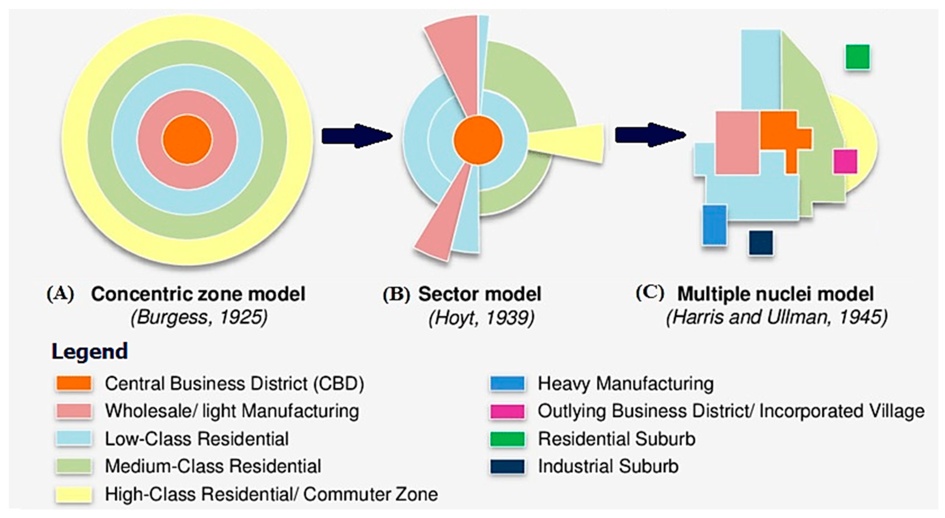
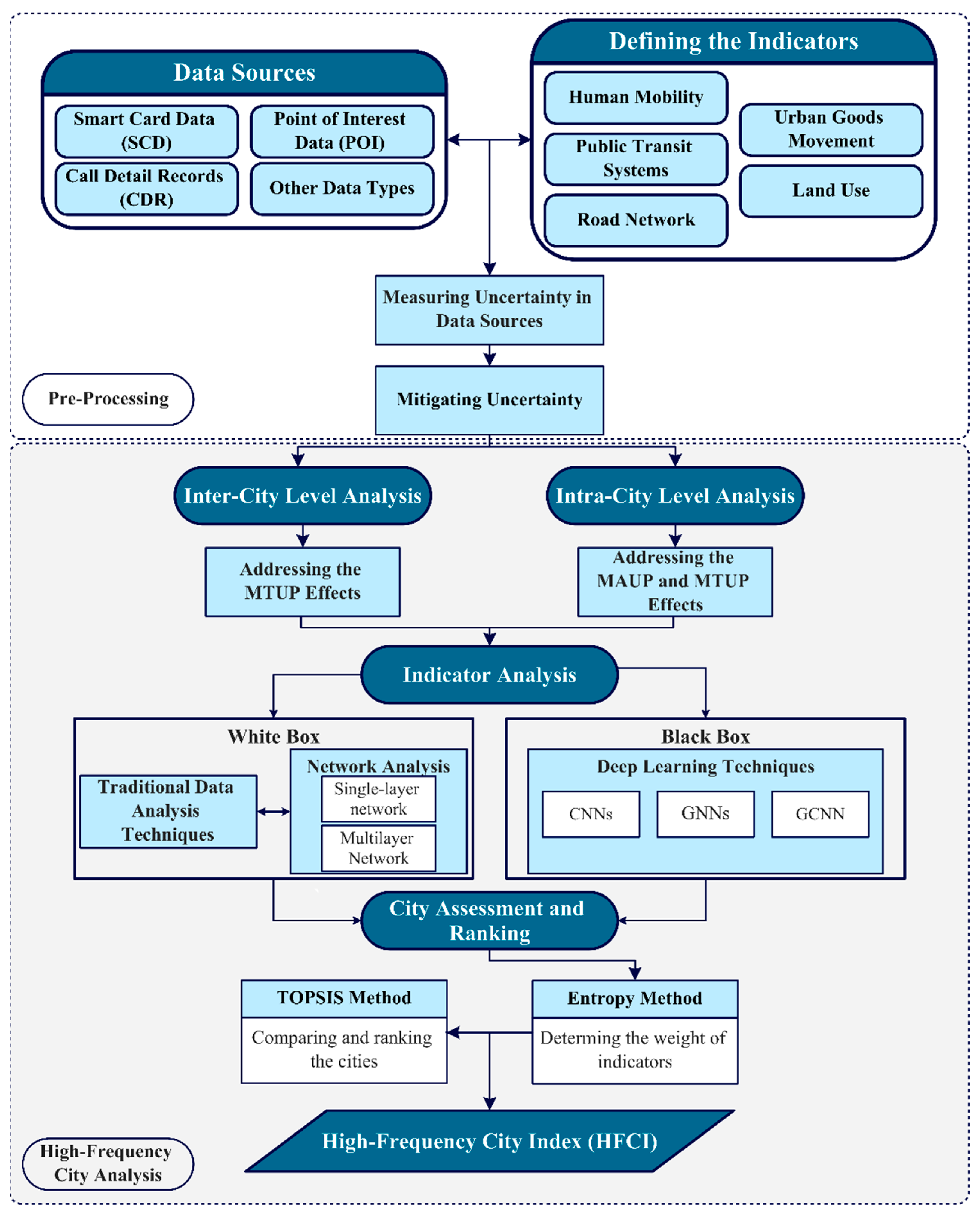
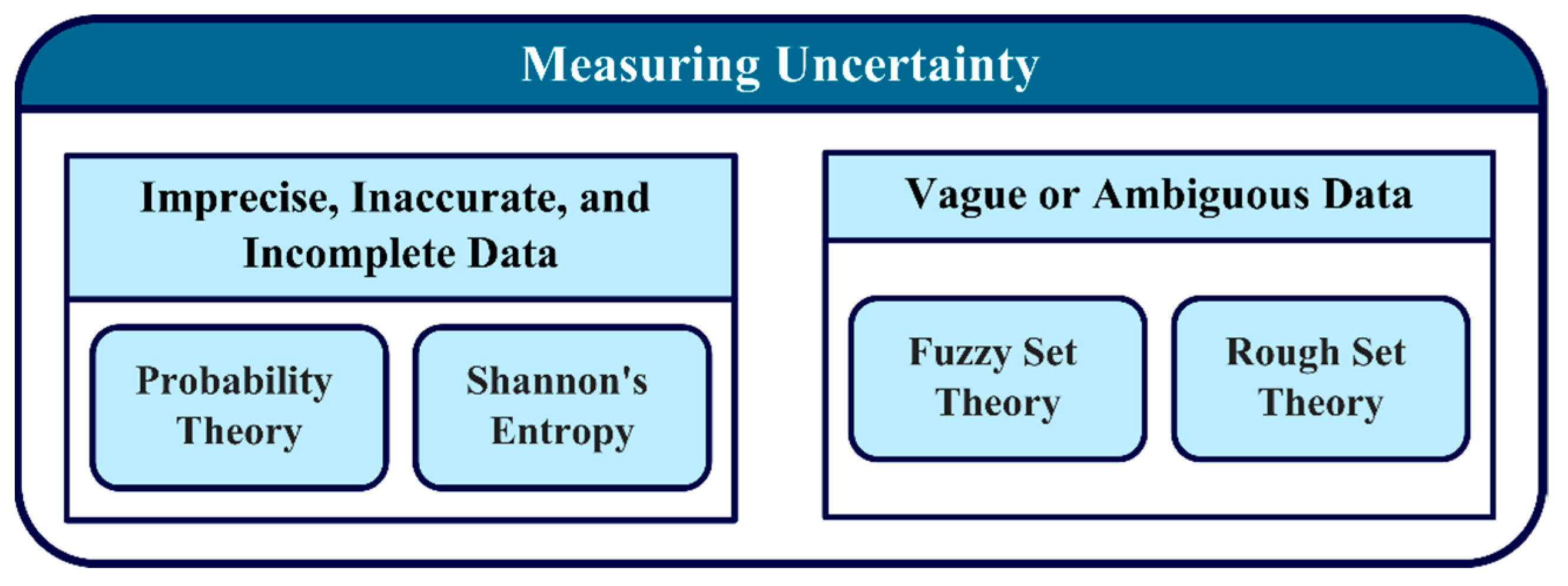
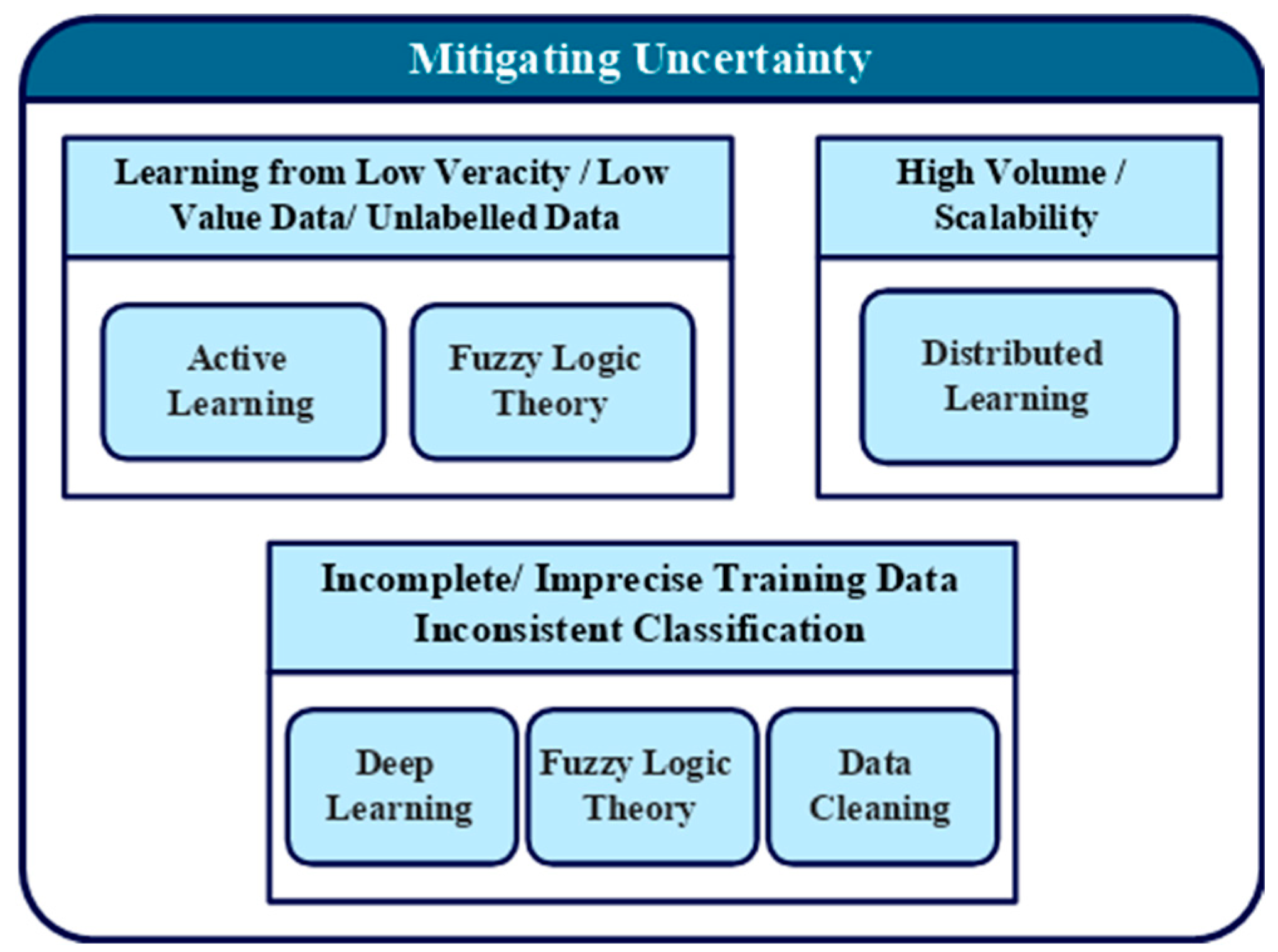
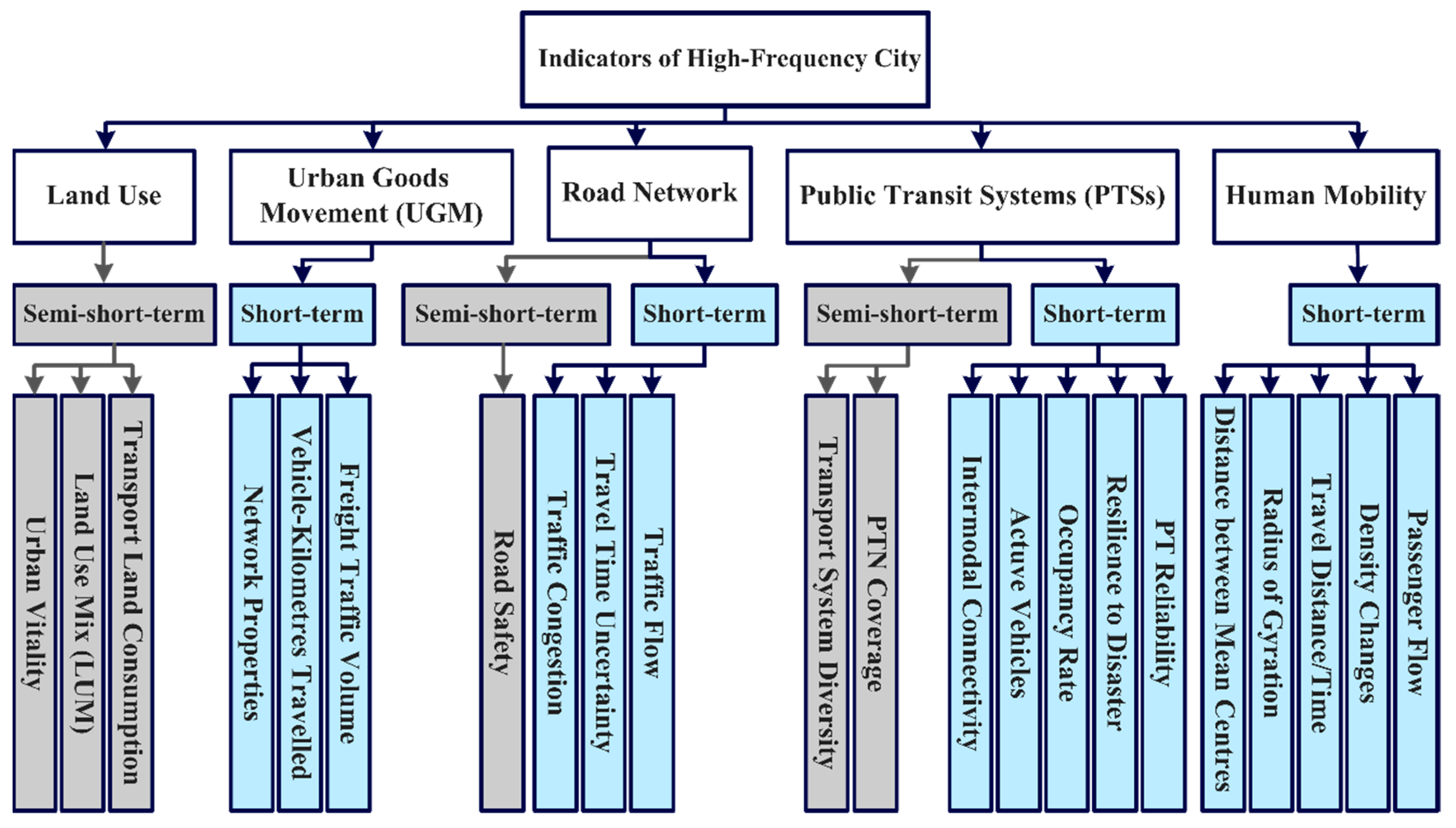
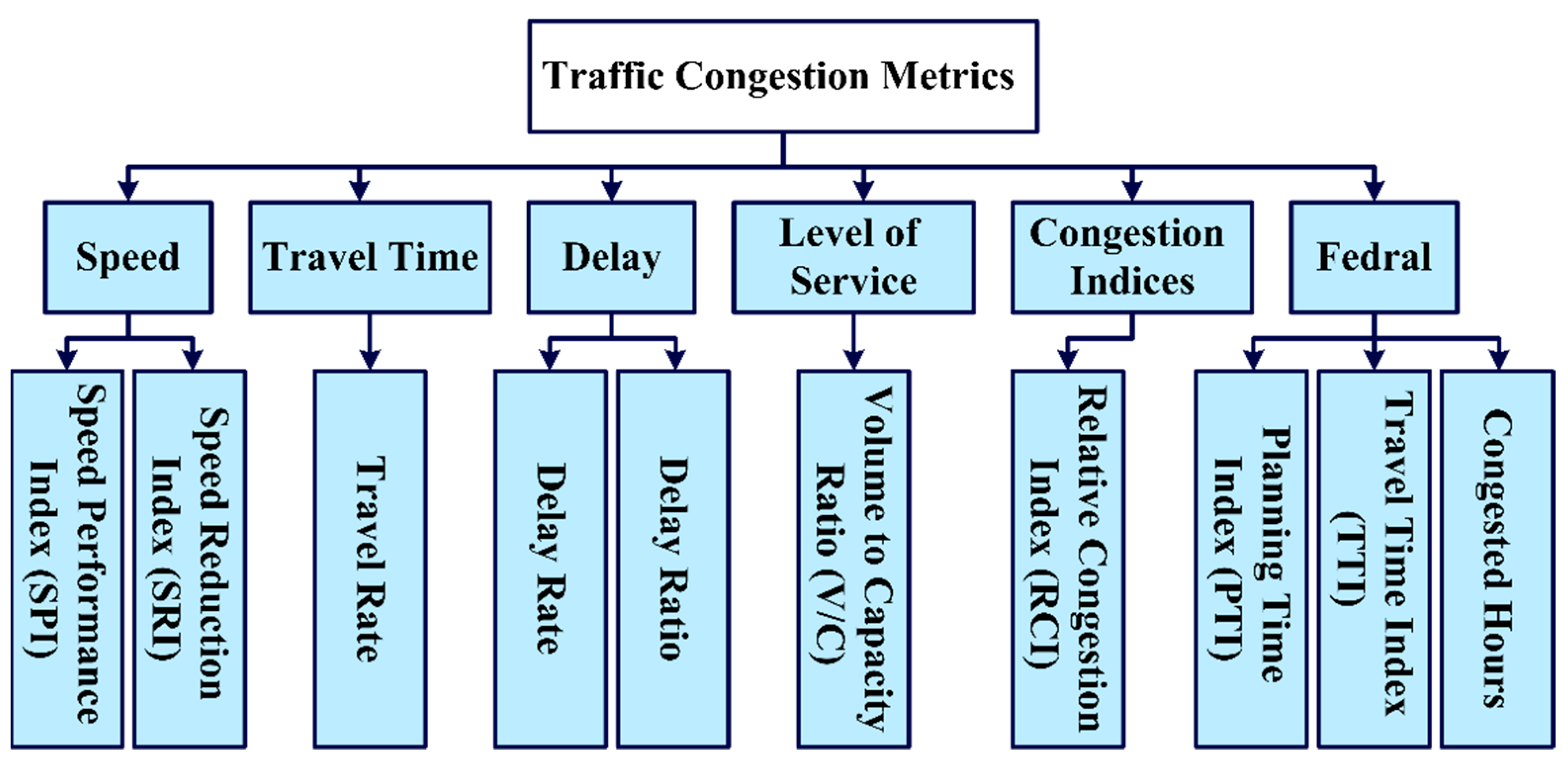
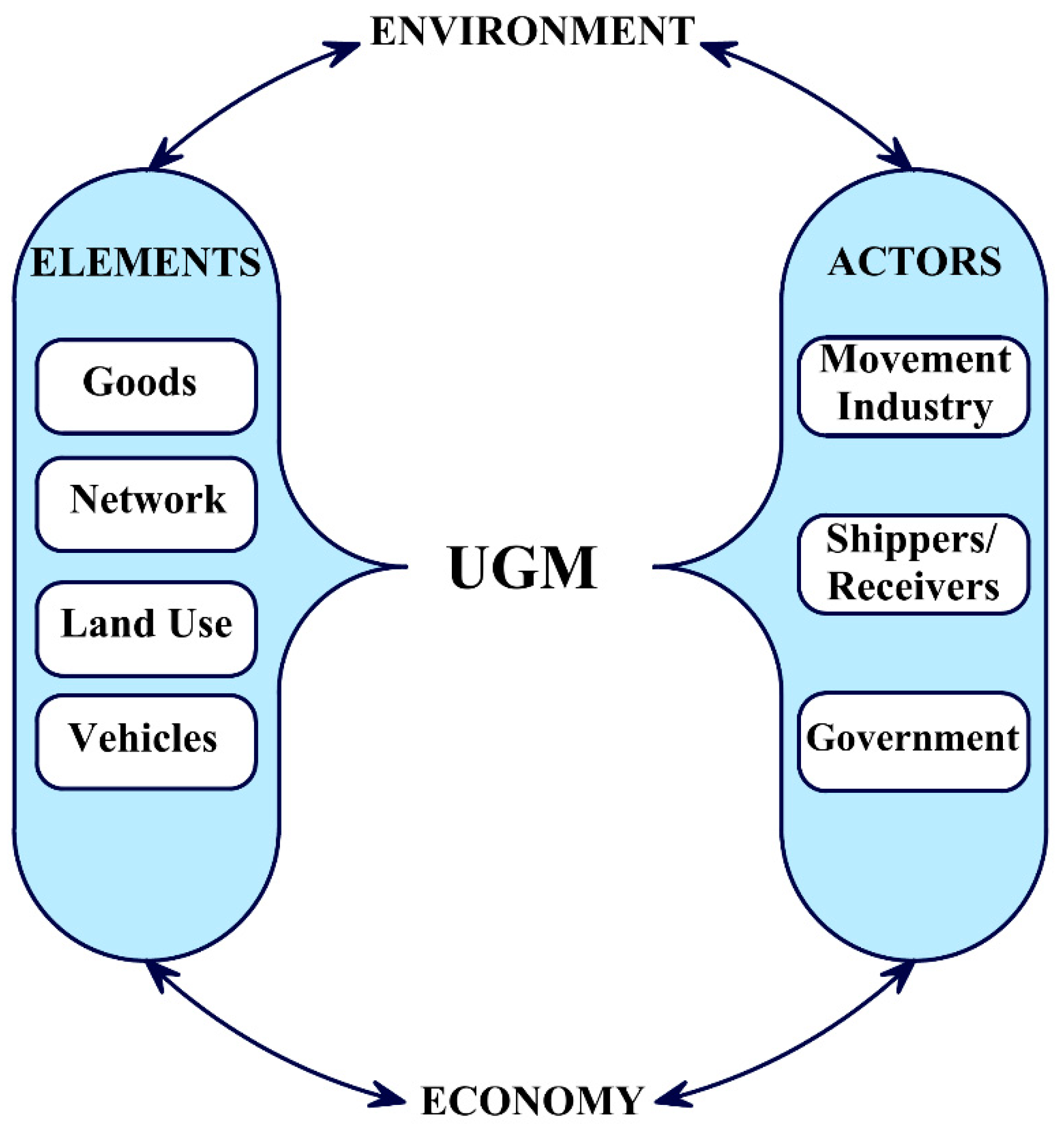
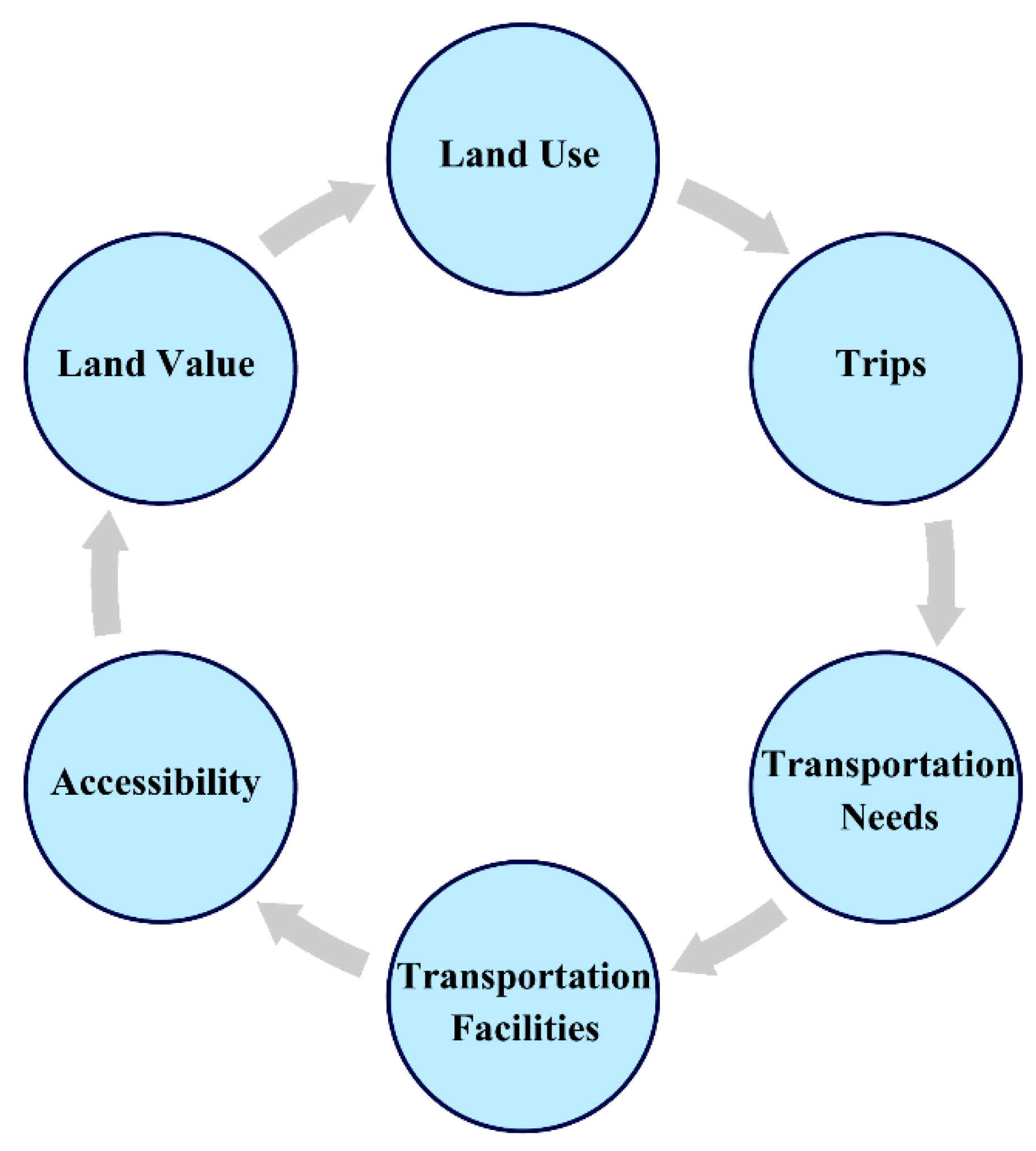
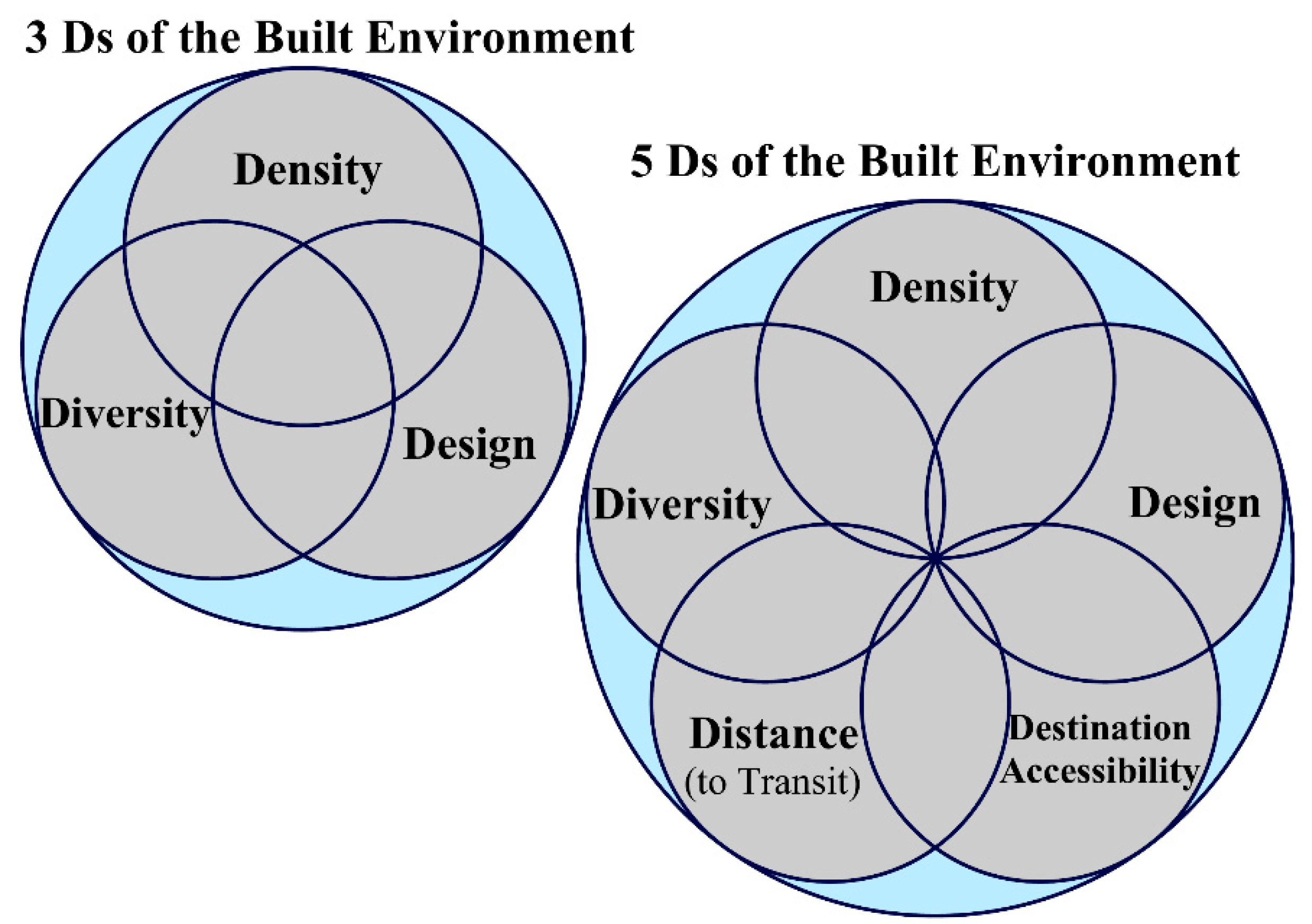
Table 1.
A list of some previous studies considered in the literature review for the selection of indicators within the period from 2010 to 2021, arranged in descending order for the year of publication, followed by ascending order for the number of indicators.
Table 1.
A list of some previous studies considered in the literature review for the selection of indicators within the period from 2010 to 2021, arranged in descending order for the year of publication, followed by ascending order for the number of indicators.
| Method, Publication Year and References | Objective of Study | Orientation of the City | Type | Categories | Extent of Application | # of Indicators/Metrics | # of Applied Cities |
|---|---|---|---|---|---|---|---|
| Sustainability Assessment of Shared Automated Electric Vehicles, 2021 ([16]) | Measuring the impacts of shared automated electric vehicles on mobility. | Sustainable City | Indicator Set | Social, Environmental, Economic and Governance | International | 20 | - |
| Mobility Performance Metrics (MPM), 2020 ([17]) | Measuring the extent to which the integrated public-private mobility system meets the needs of passengers, the performance of the system while meeting mobility on demand (MOD). | Sustainable City | Indicator Set | Connectivity, Financial Management, Planning, Environmental, Equity, Safety and Security, Customer Satisfaction, Organisational Excellence and State of Good Repair | International | 63 | 11 |
| The Deloitte City Mobility Index (DCMI), 2019 ([18]) | Evaluating the performance of a city’s mobility network and its readiness to embrace the future. | Sustainable City | Composite Index | Performance and Resilience, Vision and Leadership, Service and Inclusion | International | 15 | 57 |
| Smart Mobility Indicator (SMI), 2019 [19] | Developing an index to assess the level of "smart mobility" solutions implemented in cities. | Smart City | Composite Index | Technical infrastructure, Information infrastructure, Mobility methods and Legislation | International | 17 | - |
| Urban Mobility Indicators for Walking and Public Transport, 2019 ([13]) | Investment promotion in more accessible, safe, efficient, affordable and sustainable infrastructure for walking and public transport. | Sustainable and Liveable City | Indicator Set | Comfort and Safety, Service Demand, Connecting Destinations, Support and Encouragement | European | 34 | 8 |
| Urban Mobility Performance Indicators, 2019 ([20]) | Identifying the most used urban mobility metrics.1 | Sustainable and Smart City | Indicator Set | Accessibility, Environmental, Social, Economic, Infrastructure, Integrated Planning, Health and safety, Traffic Circulation, Urban Transportation System and Smart Mobility | International | 63 | - |
| Transportation Sustainability Indices for a Liveable City, 2018 ([21]) | Developing sustainable transport indicators for a liveable city to predict its future dynamics and formulate sustainable urban transport strategies that take into account the time dependency of the indicators. | Sustainable and Liveable City | Indicator Set | Environment, Economic and Social | National | 18 | 1 |
| Mobility Index Sustainable Urban (IMUS), 2017 ([22]) | Presenting an overview of different urban mobility indices and application of the Mobility Index Sustainable Urban (IMUS) for the public transport sector. 1 | Sustainable City | Composite Index | - | National | 22 | 1 |
| Sustainable Cities Mobility Index, 2017 ([23]) | Comparison of global mobility systems in terms of sustainable urban mobility, which includes measures for the social, environmental and economic health of the city. | Sustainable City | Composite Index | People, Planet and Profit | International | 23 | 100 |
| Indicators for Sustainable and liveable Transport Planning, 2017 ([24]) | Providing guidance on the use of indicators for sustainable and liveable transport planning. 1 | Sustainable and Liveable City | Indicator Set | Economic, Social, Environmental, Good Governance and Planning | International | 40 | - |
| Citykeys Indicators For Smart Cities, 2017 ([25]) | Monitoring the evolution of a city towards an even smarter city. | Smart City | Indicator Set | People, Planet, Prosperity and Governance | European | 76 | - |
| Sustainable Urban Mobility Indicators, 2017 ([26]) | Providing a literature review and selection of urban mobility indicators for Thessaloniki city. | Sustainable City | Indicator Set | Integration of Land Use, Accessibility, Mobility, Promotion of Non-Motorised Means, Encouragement Of PT, Environmental Concerns, Economic Welfare and Road Safety | National | 80 | 1 |
| Sustainability Measures of Urban Public Transport, 2016 ([27]) | Assessing the sustainability of public transport systems. | Sustainable City | Indicator Set | Environment, Social, Economic and System Effectiveness | Middle East/Asia | 15 | 26 |
| Sustainability Compound Index (SCI), 2012 ([28]) | Assessing and prioritising transportation sustainability strategies in Taipei city. | Sustainable City | Composite Index | Society, Economy, Environment, Energy and Finance | National | 10 | - |
| Indicators for Sustainable Urban Mobility, 2012 ([29]) | Developing a set of urban mobility indicators to show the driving forces behind the evolution of transport volumes and modal split and to assess the performance of transport and environmental policies. | Sustainable City | Indicator Set | Population, Economy, Urban structure, Transport, Environment and Policy | National | 43 | 21 |
| Transport Sustainability Index (TSI), 2011 ([30]) | Providing a hybrid approach based on the Analytical Hierarchy Process (AHP) and Dempster–Shafer theory to assess the impact of green transport measures on the sustainability of a city. | Sustainable City | Composite Index | Society, Transport, Environment, Energy and Economy | International | 19 | - |
| Index of Sustainable Urban Mobility (I_SUM), 2010 ([31,32,33]) | Evaluating and comparing the mobility condition of cities. | Sustainable City | Composite Index | Accessibility, Environmental, Social, Political, Transport Infrastructure, Non-Motorised Modes, Integrated Planning, Urban Circulation Traffic and Urban Transport Systems. | National | 87 | 6 |
1 The document presented examples of applied sustainability indicator set or various sustainability indices in various studies.
Table 2.
The distribution of included documents in the literature databases.
| Journal Articles | Conference Papers | Books/Book Chapters | Reports | Theses | Total | |
|---|---|---|---|---|---|---|
| Database for Smart/Sustainability Assessment | 34 | 4 | 1 | 18 | 0 | 57 |
| Database for Exploring Human Mobility Pattern | 56 | 8 | 0 | 0 | 0 | 64 |
| Database for Reviewing metrics of the Selected Indicators | 96 | 8 | 3 | 9 | 1 | 117 |
| Database for Understanding the Complexity of the City | 74 | 6 | 13 | 4 | 1 | 98 |
| Total | 260 | 26 | 17 | 31 | 2 | 336 |
Publisher’s Note: MDPI stays neutral with regard to jurisdictional claims in published maps and institutional affiliations. |
© 2021 by the authors. Licensee MDPI, Basel, Switzerland. This article is an open access article distributed under the terms and conditions of the Creative Commons Attribution (CC BY) license (https://creativecommons.org/licenses/by/4.0/).
Share and Cite
MDPI and ACS Style
Senousi, A.M.; Zhang, J.; Shi, W.; Liu, X. A Proposed Framework for Identification of Indicators to Model High-Frequency Cities. ISPRS Int. J. Geo-Inf. 2021, 10, 317. https://doi.org/10.3390/ijgi10050317
AMA Style
Senousi AM, Zhang J, Shi W, Liu X. A Proposed Framework for Identification of Indicators to Model High-Frequency Cities. ISPRS International Journal of Geo-Information. 2021; 10(5):317. https://doi.org/10.3390/ijgi10050317
Chicago/Turabian StyleSenousi, Ahmad M., Junwei Zhang, Wenzhong Shi, and Xintao Liu. 2021. "A Proposed Framework for Identification of Indicators to Model High-Frequency Cities" ISPRS International Journal of Geo-Information 10, no. 5: 317. https://doi.org/10.3390/ijgi10050317
Note that from the first issue of 2016, this journal uses article numbers instead of page numbers. See further details here.