
On the Relationship between Generalization and Robustness to Adversarial Examples


VISILAB, University of Castilla La Mancha, ETSII, 13071 Ciudad Real, Spain
*
Author to whom correspondence should be addressed.
Symmetry 2021, 13(5), 817; https://doi.org/10.3390/sym13050817
Submission received: 23 March 2021
/
Revised: 9 April 2021
/
Accepted: 30 April 2021
/
Published: 7 May 2021
Abstract
:One of the most intriguing phenomenons related to deep learning is the so-called adversarial examples. These samples are visually equivalent to normal inputs, undetectable for humans, yet they cause the networks to output wrong results. The phenomenon can be framed as a symmetry/asymmetry problem, whereby inputs to a neural network with a similar/symmetric appearance to regular images, produce an opposite/asymmetric output. Some researchers are focused on developing methods for generating adversarial examples, while others propose defense methods. In parallel, there is a growing interest in characterizing the phenomenon, which is also the focus of this paper. From some well known datasets of common images, like CIFAR-10 and STL-10, a neural network architecture is first trained in a normal regime, where training and validation performances increase, reaching generalization. Additionally, the same architectures and datasets are trained in an overfitting regime, where there is a growing disparity in training and validation performances. The behaviour of these two regimes against adversarial examples is then compared. From the results, we observe greater robustness to adversarial examples in the overfitting regime. We explain this simultaneous loss of generalization and gain in robustness to adversarial examples as another manifestation of the well-known fitting-generalization trade-off.
1. Introduction
Research in machine learning has experienced a great advance since the advent of deep learning. This methodology is able to learn meaningful features to classify, generate or detect objects in images, audio or any kind of signal. The results obtained with this framework are outstanding, although their behaviour remains like a black box. Also, striking errors appear in some specific cases, like in the case of the so-called adversarial examples.
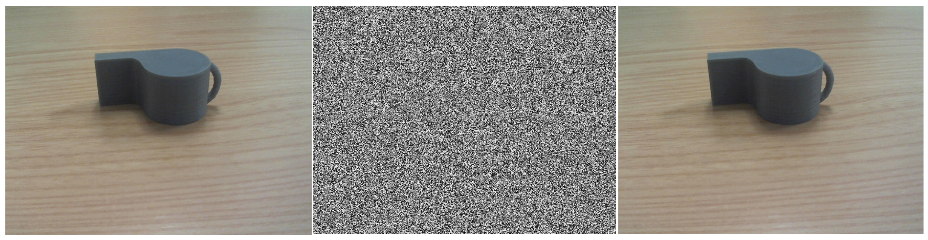
Adversarial examples are carefully perturbed inputs to a machine learning system that, even though they seem very similar to the original examples, produce a response in which the output is incorrect. For example, Figure 1 shows an image which, with a small perturbation, is classified as a screw rather than a whistle, which is obviously an error for us humans [1].
Note that the phenomenon can be interpreted as a symmetry/asymmetry problem, whereby inputs to a neural network with a similar/symmetric appearance to regular images, produce an opposite/asymmetric output.
Several attacks (algorithm to produce adversarial examples) and also defenses (methodologies to make networks more robust against adversarial examples) have been developed. On the one hand, the most successful attack methods are the ones proposed in [2,3,4]. Most of them compute variations on the input images to modify the gradient computed in the network, so that the output points to a different class. As for defense methods, their purpose is to modify the training methodology, or the network architecture, so that the produced models are more robust to these perturbations. Some of the most popular are: Adversarial Training [5], which proposes data augmentation with adversarial examples to train the network on their features; Pixel Defend [6] which modifies the image pixels to fit them to the training pixel distribution and “undo” the perturbations; and the so-called Defensive Distillation [7]. In the latter method, the encoded and predicted class probabilities of a neural network classifier are used to train a new network that increases its robustness with respect to the original.
Apart from research into defense and attack methods, there is a body of research focused on characterizing the phenomenon of adversarial examples. Some of the research in this line have suggested the well-known generalization versus memorization trade-off as a cause for this problem [8]. Training a model to achieve good generalization (high performance on unseen examples) decreases robustness to adversarial examples and vice versa.
Let us consider a thought experiment in which the test subset is composed by samples generated by crafting adversarial examples from the training set. Even though those adversarial examples are perceptually close to the training set, they are nonetheless valid test (i.e., unseen) samples. On the other hand, overfitting to the training samples is general bad for generalization. However, since the adversarial examples can be arbitrarily close to the original samples, overfitting should also have a positive effect on these adversarial examples. In fact, following the same reasoning, as the number of training samples tend to infinity *any* adversarial example should benefit from overfitting. Thus, there are indeed reasons that suggest that at least for certain cases robustness to adversarial examples can benefit from overfitting.
Some works, like in [9], argue that adversarial examples manifestation crafted on different architectures and disjoints datasets indicates that overfitting is not related to the cause of this phenomenon. However, Refs. [10,11] support that weigh decay and regularization can help to increase robustness to adversarial examples, supporting the implication of overfitting. Other works show that adversarial examples exploit the features that are learned by the model [12]. In the latter work, it is stated that neural networks learn their own features to classify the data. The features selected by neural networks are usually not the same as the human perception patterns. Moreover, they study the presence of robust and non-robust features, and propose a methodology to build datasets taking this into account. Forcing the models to learn the robust features increases adversarial robustness. Other findings to explain this phenomenon point in the direction of the non-linearity of the layers employed in the network architectures [1].
In [13], it is shown that overfitted models have stronger adversarial robustness, at the cost of lower generalization. However, their methodology presented some problems, since they did not study the evolution of adversarial robustness during all the epochs in the training process, only in the first and last epoch. Moreover, a comparison with a non overfitting regime is not considered. In this paper, we extend their experimentation, considering the progression of adversarial example robustness in two training regimes: normal (validation-error reduction) and overfitting, monitoring the whole training process to study the robustness trends.
Finally, Ref. [14] performs a comprehensive study of robustness for different models in the ImageNet dataset. This work considers robustness and accuracy in final models, that is, in the last epoch of a training process, where maximum accuracy is obtained for the validation dataset. As a result, a comparison is performed among different families of architectures. The main conclusion is that models in which validation accuracy is lower and architecture complexity is also limited (Alexnet, MobileNet) are more robust in comparison to more complex networks in which validation accuracy is higher (such as Inception or DenseNet).
In our work, we focus on the trade-off that is established between accuracy and robustness at different training epochs for the same model. Moreover, two different regimes are forced in the training process. One, in which a “normal” training is performed (as in [14], looking for the maximum validation accuracy) and another in which the model is trained in an overfitting regime (validation accuracy drops at certain point, while training accuracy keeps increasing). With the latter regime, the method is able to obtain a model that is more robust against adversarial examples, at the cost of decreased test performance.
The contributions of this paper are the following. Extensive experimentation has been performed to show the different behaviour of neural networks when they are trained in both a normal and overfitted regime. Different attack methods are considered, from the most popular and robust in recent research. To support the experimentation, some metrics are calculated to compute the adversarial robustness of the models, in order to show the relationship of these metrics to the hypothesis presented in [13], which is also supported in our work.
This paper is organized as follows: Section 2 presents the datasets employed in this work and an introduction is given to the different attack methods and robustness metrics. Section 3 explains in detail the different experiments that are carried out, analyzing the obtained results. Finally Section 4 outlines the main conclusions.
2. Material and Methods
In this section, the materials employed in this work are detailed. In this case, CIFAR-10 and STL-10, common reference datasets in computer vision, are selected to perform the study. The main attack methods developed in current research are studied and defined below. Also, relevant model robustness metrics and image distance metric are commented.
2.1. Datasets
In work with adversarial examples, it is common to use datasets like MNIST [15], which covers a collection of grayscale handwritten digits with 28 × 28 pixel size, suitable for automatic recognition system development. Other variants are proposed in [16], which was developed to build a similar result than the obtained originally, with a much more extensive test set. Finally, others like Fashion-MNIST (developed by the Zalando company in [17]), are being increasingly used. This one consists of thumbnails of grayscale cloth images, in a similar structure and size than the previous ones.
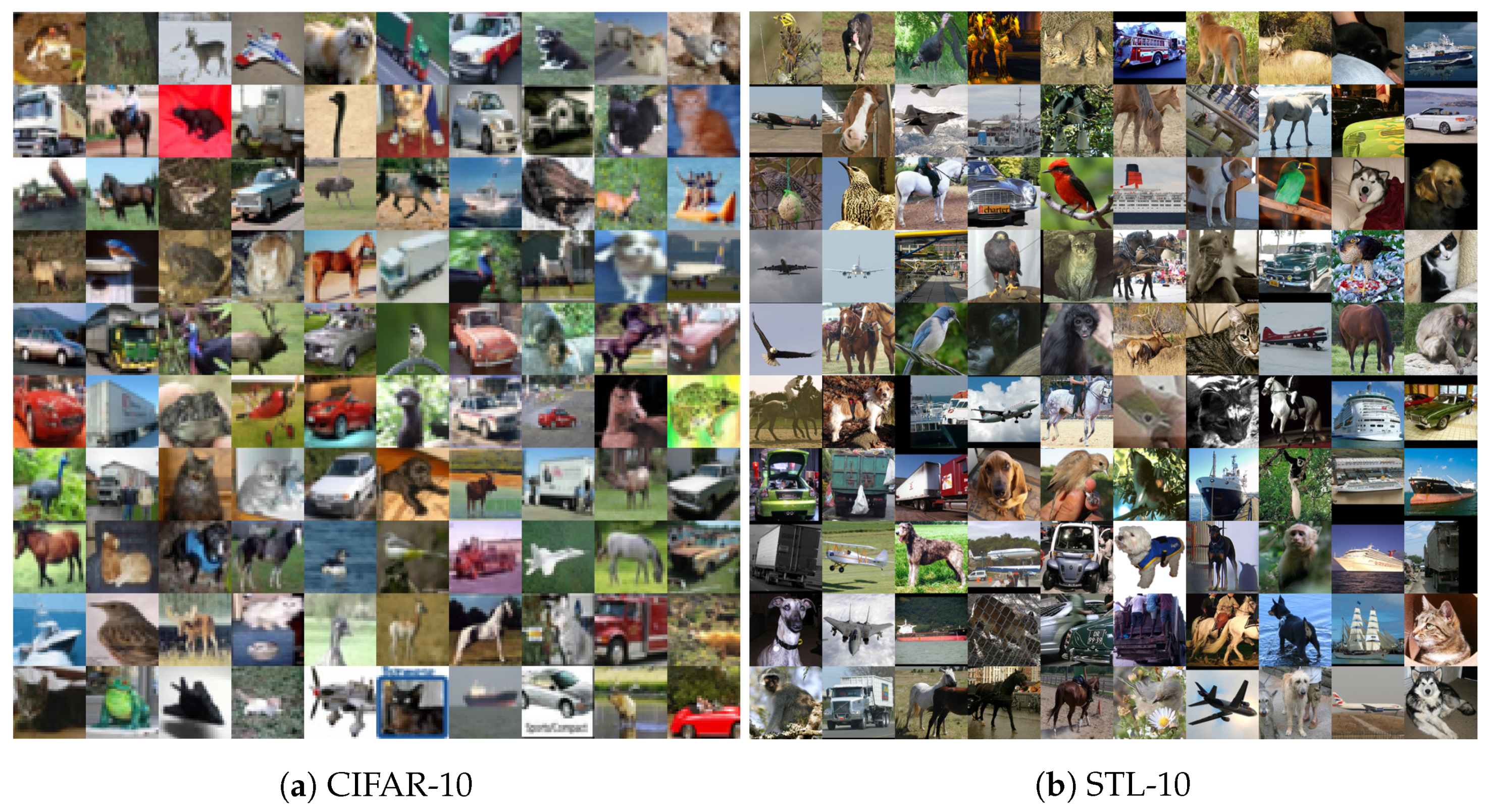
However, in this work, we start directly with more real-world like images, suitable for a wider range of applications. For this reason, the STL-10 dataset [18] has been chosen as the main dataset for this work. The images have a limited size of 96 × 96 × 3 pixels (RGB color), and were taken from labeled examples for the ImageNet by [19] dataset, with samples from 1000 different categories. An example is shown in Figure 2.
As a first step, initial experimentation is also performed with a smaller and similar dataset as CIFAR-10, from [20], to show if the hypothesis in this work is promising in an early step. Both datasets represent 10 different categories from common objects and animals from real-world images: airplane, bird, car, cat, deer, dog, horse, monkey, ship and truck. Note that images in CIFAR-10 are smaller (32 × 32 × 3) than the ones of STL-10, as shown in Figure 2. Finally, note that in CIFAR-10 there are 50,000 images for training and 10,000 for testing, while STL-10 dataset has 5000 images available for training and 8000 for testing, which makes it more challenging.
2.2. Methods
There are different methods to craft adversarial examples from a given input, so-called attacks. Most of them are based on the gradient variation response so that the model classifies the image with a different output. They can be targeted or untargeted. That is, whether they force the adversarial to be predicted as a specific class or not. In the latter case, the algorithms usually select the easiest to fool or a random class. A brief description of the adversarial attack methods used in the experiments for comparison can be found in [21]. The main methods that are considered in this work are: FGSM [9], Carlini & Wagner [2] and PGD [4] (derived from Basic Iterative Method [22]).
2.3. Metrics
Another important aspect of our work is the ability to measure the adversarial robustness of a model. These algorithms need a trained model and some test examples (the more examples, the better the precision, but more computational time is required). For this purpose, different metrics are proposed:
- Loss Sensitivity: proposed in [8] it computes the local loss sensitivity estimated through the gradients of the prediction. It measures the effect of the gradients for each example, which translates into a measure of how much an example is memorized. The larger the value, the greater the overfitting to this particular example.
- Empirical Robustness: as described by [23], it is equivalent to computing the minimal perturbation value that the attacker must introduce for a successful attack, as estimated with the FGSM method.
- CLEVER: elaborated in [24], this metric computes a lower bound on the distortion metric that is used to compute the adversarial. It is an attack-agnostic metric in which, the greater the value, the more robust a model is supposed to be.
Also, it is important to compare the difference between the crafted adversarial examples and the original examples. For this purpose, the main metrics that are used are based on the norm, calculated over the difference between the original and the adversarial example. The most common variants of this metric are shown in Table 1.
3. Experimental Results and Discussion
Two different experimental set-ups are proposed. The first one is performed in a no-overfitting regime and the second one in an overfitting regime. For each experiment, a cross-validation procedure is set up. The training dataset is distributed into 5 training/validation folds. The models are trained using 4/5th parts of the training set and validated with the remaining fifth. This procedure is repeated 5 times, rotating the part that is left out for validation. For each run, an optimal model is selected according to the accuracy on the validation dataset. Then, adversarial examples are crafted on the test set for each method against the selected snapshot. To evaluate the results, the Adversarial Successful Rate (ASR) is computed, which is defined as “1—accuracy” obtained by the model for each adversarial set. The accuracy for the original test samples is also provided. Also, the distance metrics and adversarial robustness metrics described above are computed to show the difference in the behaviour between both regimes. This process is performed for each fold of the cross-validation scenario.
In order to show the results for the different runs, each line in the plots represents the mean value obtained at each epoch. Additionally, vertical lines are included to represent one standard deviation of the means. Analogously, when results are provided numerically in tables, they also contain the mean and standard deviation.
3.1. No Overfitting
The first set of experiments is performed using appropriate parameters to reduce the validation error. This is usually the main goal when training a model for a specific task. In consequence, the generated model is expected to generalize, being able to perform accurately for samples that are not present in the training dataset, while they keep on the same distribution, known as the test set.
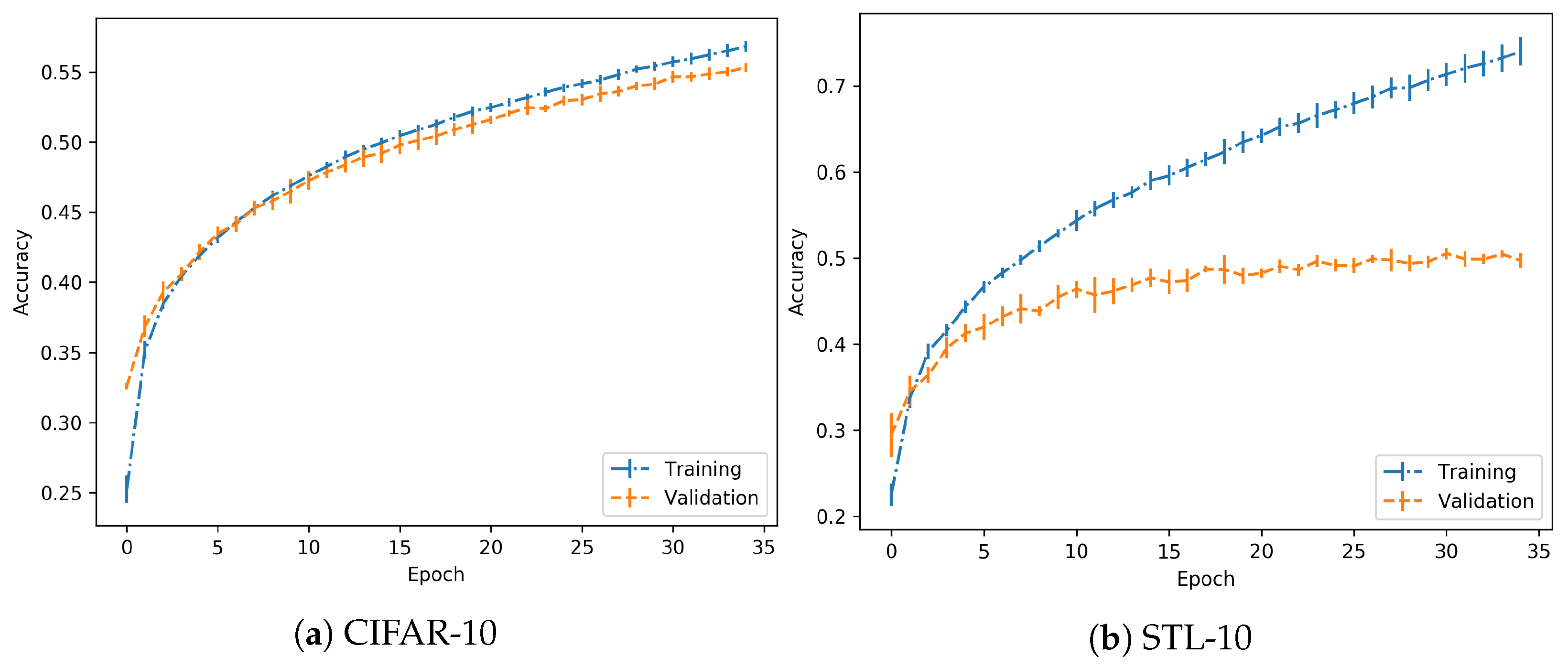
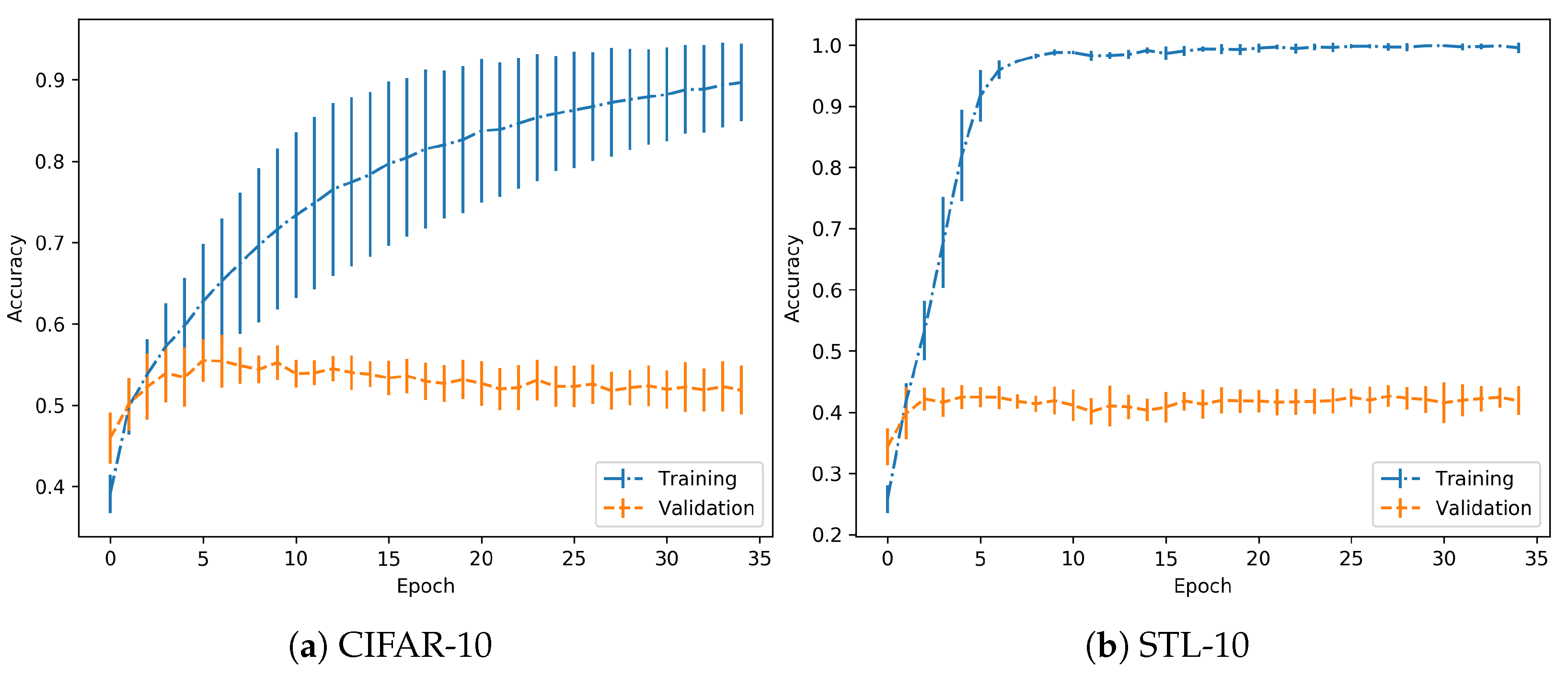
In the case of the CIFAR-10 dataset, training has been performed using a LeNet architecture as described in [25], implemented in a Keras-Tensorflow backend. Training was performed for 35 epochs and with a learning rate of . The performance is shown in Figure 3. The important key is to check that both training and validation accuracies grow with the same positive progression.
Considering the results for the previous dataset, in the case of the STL-10 dataset, the same set-up and parameters are employed. Performance is shown in Figure 3. As in the previous case, it is observed that the achieved models are trained with no overfitting. So, in both cases, they are suitable to continue with the experimentation.
Regarding the performance on the training process, it should be noted that the objective is to clearly differentiate between normal and overfitting regimes, independently of the absolute values in validation accuracy, for example. As suggested in the experimental proposal, when the model is trained on a normal regime, the validation accuracy increases progressively, which is achieved here. However, in the overfitting regime, this accuracy should reach a peak and then start dropping, as observed in further experimentation. In both cases, the images used for adversarial generation are correct predictions for the given model, so there is no drawback in discarding some of the images due to low relative nominal test performance. Specifically, the STL-10 dataset has a wider difference between training and validation accuracy, but the trends persist.
In this case, the models trained in this non-overfitting regime have been tested against the CW, FGSM and PGD attack methods for both datasets (CIFAR-10 and STL). In all cases, they have been set up to perform untargeted attacks (with no predefined destination class) using distance metric to generate the adversarial examples. Moreover, the minimum confidence value parameter is given to CW, and standard maximum perturbation of 0.3 are set-up for PGD and FGSM.
The epoch with the best validation accuracy is selected to craft the adversarial examples. Then the rest of models are applied over the same adversarials. Here we are leveraging a concept known as adversarial transferability [26]. The architecture remains the same but with increasing/decreasing levels of generalization through the training process. For this reason, the adversarials are considered to be highly transferable and, therefore, suitable to study their effects on different stages of the training and with different parameter conditions (overfitted vs regularized).
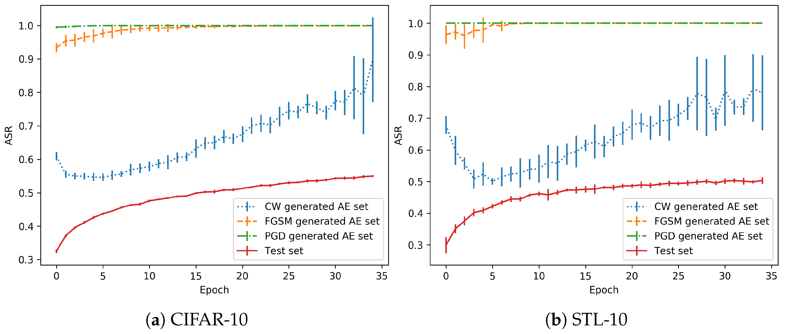
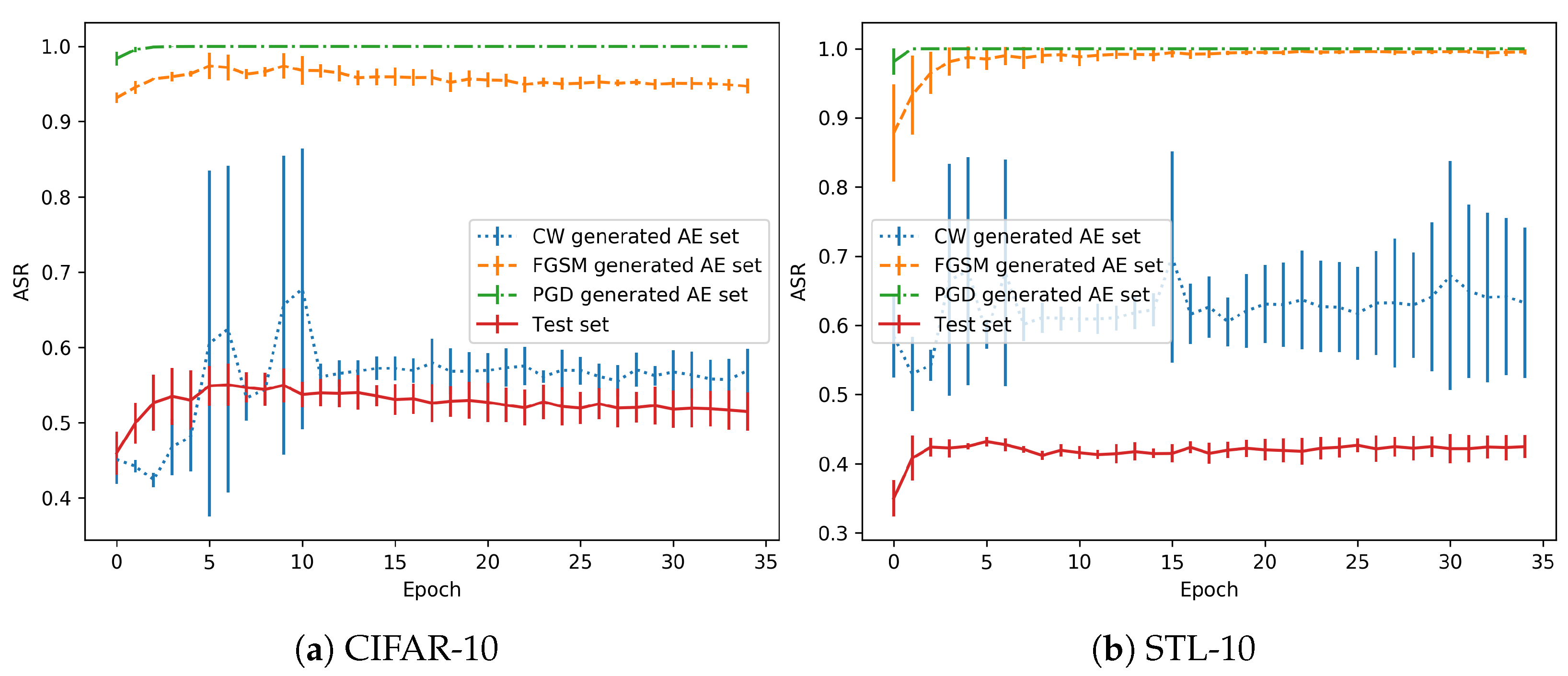
As the training is performed in a normal regime, the 35th and last epoch is usually the one with the best validation accuracy, see Figure 3. The adversarial examples generated with each method are classified with the snapshot models trained with all the epochs. Then, the accuracy in each AE (Adversarial Example) set is obtained. Figure 4 shows the test accuracy curve and the Attack Success Rate (ASR), for the attacks that have been performed. This metric represents the percentage of adversarials that are misclassified by the model.
As shown in the performance of the CW attack for these models, the adversarial success rate is lower in the first epochs (from the 5th epoch onwards, as the previous ones should not be considered as the models are not stable), when the model is still a bad classifier. However, when the test accuracy increases, the performance of the model in the AE set drops significantly. There is a remarkable trend that shows that, when the model is well trained for generalization, the effect of adversarial perturbations is stronger.
Regarding the differences between the CW attacks and FGSM/PGD, the former is the best in terms of the quality of the generated adversarials. That is, they are the most similar to the originals images (in terms of metrics). However, in terms of robustness, they can be discovered with small changes in the decision boundary, as will be shown with the overfitting models (and also happens here with the normal regime). Depending on the training state, a better generalization can also point to adversarials that fall in the same distribution if they are very close. However, the other two attacks obtain a greater success rate because the adversarials are crafted with a larger distance from the test distribution, as observed for both (Euclidean distance) and (maximum perturbation) metrics.
Table 2 shows the performance of the CW method with the CIFAR-10 models. First, the metric shows the total number of pixels modified by mean. The maximum value would be 1024 (32 × 32), so more than 98% of the pixels have some alteration from the original image. However, they are modified with very low values, as shown by (Euclidean) distance and especially by the very low maximum perturbation indicated by metric. This metric indicates the maximum perturbation added to the intensity of any pixel in the image, considering that they are represented in a range of 0–1.
Table 3 shows the AE distances with respect to the original test set for STL-10. The PGD and FGSM AE sets consistently fool the model during the whole training process, as seen in the previous curve. This is produced because, as this table points out, the adversarials generated by these methods are farther away (from the original test samples) in comparison with the examples generated by CW. With distances ranging from 23–26, against 0.97 on average by CW, this means that the adversarials are too far. Instead, CW examples achieve good ASR with potentially undetectable adversarials. Considering the size of the images in this dataset (98 × 98 = 9604), more than the 90% of the pixels are modified in comparison with the original test images (see distances in Table 3). The maximum perturbation, calculated in distance, is 0.30 for FGSM-PGD (which is expected as it is bounded by a parameter of the adversarial methods), while CW has a smaller value, with 0.06. These results also point in the same direction as the previous statements, supporting the notion that the improvement in generalization also leads to worsening results for AEs that are closer to the originals. In other words, as the models achieve better generalization, robustness to the best AEs (which are very close to the original) decreases.
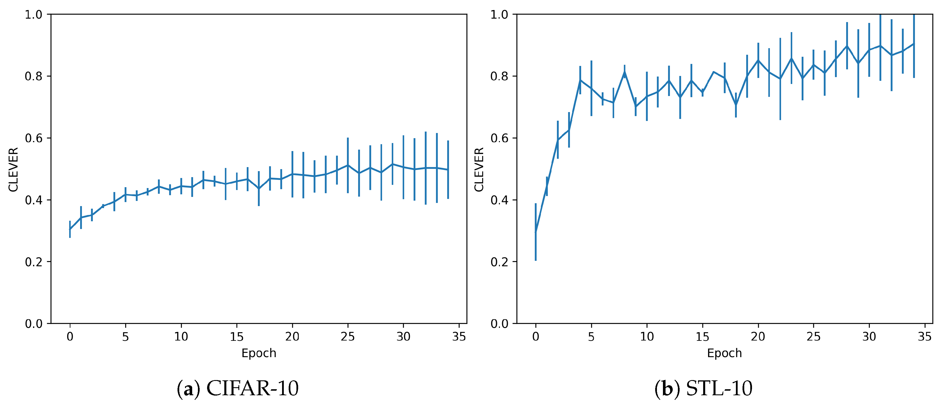
The dataset and trained models are also evaluated in terms of their adversarial robustness, using the metrics explained in Section 2.3. For the CLEVER metric, Figure 5 shows the evolution of the adversarial robustness score, depending on the epoch considered. It also shows how the robustness score increases in the sequence of epochs, but in a slight amount for the CIFAR dataset. In the case of STL, the models would be robust to higher perturbations, as the values are closer to 1. However, adversarials with further distance metrics would be sufficient to fool these models.
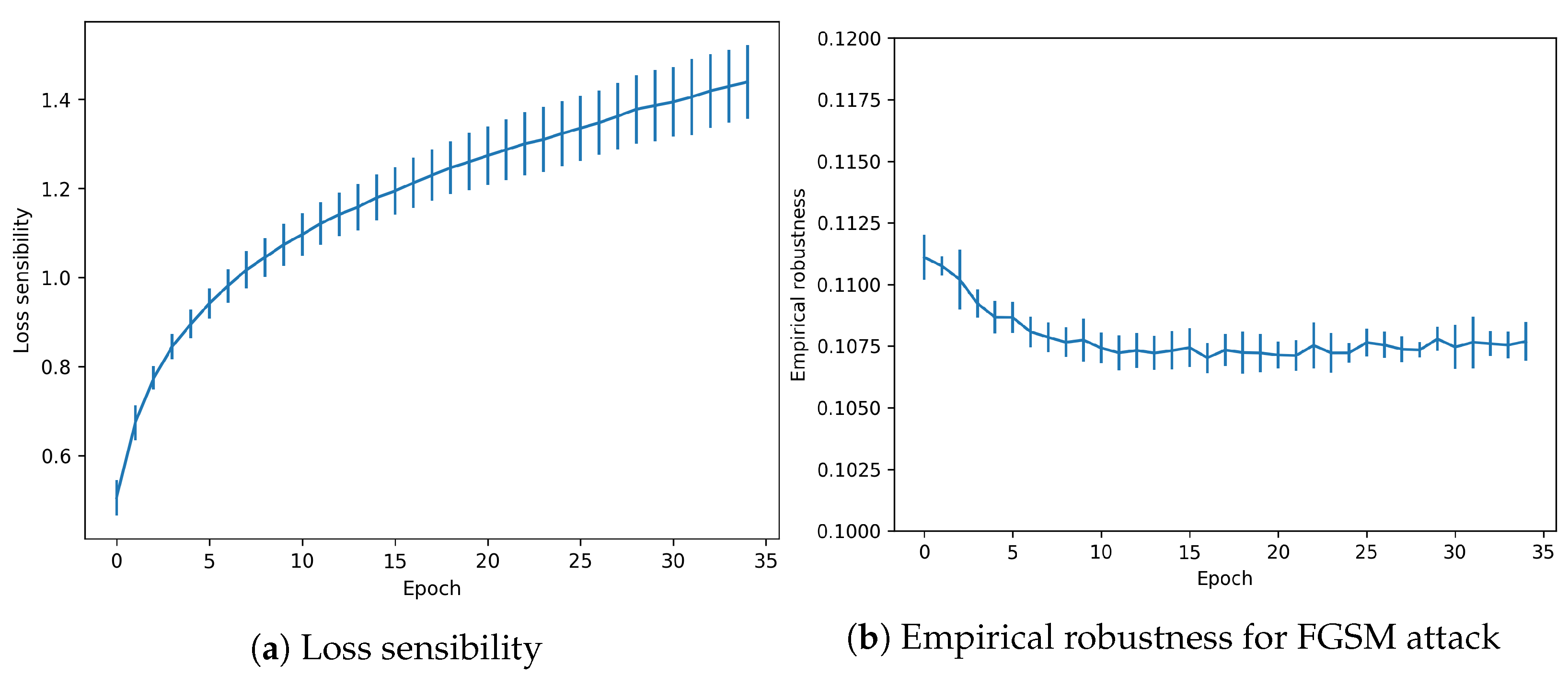
Another attack-agnostic metric is evaluated for the trained snapshots. Loss sensibility measures robustness against changes in the gradients. As shown in Figure 6, the effect is increased when the model is more accurate in the test data. However, it reaches a peak around 1.4, which is a relatively low value.
Finally, Empirical robustness shows the minimal theoretical perturbation needed to fool the model (in a FGSM attack). As shown in Figure 6, the value remains constant for the whole training process, with a low decreasing tendency.
3.2. Overfitting
This set of experiments is performed using parameters that force the model to overfit the input data. This is usually avoided when training a model for a specific task, and in fact, several techniques have been developed to prevent that (data augmentation, dropout layers, ...). With this regime, the generated model closely fits the training data, exhibiting poor performance for unseen images.
In this case, the network architecture remains the same, but the learning rate is set at 0.0024, which is found to be a suitable value to induce the models to overfit. In general, the overfitting susceptibility of a model depends on several factors (dataset, network architecture, level of regularization applied, learning rate, number of epochs...). In principle, letting training run for a large number of epochs should be a way to get to overfitting. However, the computational cost of this is very high. Therefore we decided to run our experiments with a fixed number of epochs and vary the learning rates. A high learning rate helped us reach, in a reasonable time, a behaviour similar to what would be obtained for a large number of epochs with a low learning rate. The performance for both datasets is shown in Figure 7.
In comparison to Figure 3, there is a supposed improvement in the performance for both CIFAR-10 and STL-10, since stabilized values of training accuracy around 0.9 and 1.0 are obtained. However, this is induced by overfitting. The models exhibit good performance in the training set, and bad performance on the validation set. The accuracy on the latter tends to decay from the fifth epoch, which is a clue that the models are in an overfitting state. In comparison with the no-overfitting regime, the performance curves do not follow the same tendency in training and validation.
The models trained in overfitting regime have been also tested against the CW, FGSM, PGD attack methods. As in the previous experiment, they have been set up to perform untargeted attacks using distance metric to generate the adversarial examples.
In the same way, the epoch with the best validation accuracy is selected to craft the adversarial examples over the test set. In this case, this is usually at the 5th to 10th epoch. Then, the architecture is tested in all the snapshots for the crafted adversarials. Figure 8 shows the test accuracy curve in comparison with the ASR of the adversarial attacks.
Again, PGD and FGSM adversarial examples consistently fool the model during the whole process. All the methods have greater ASR values for the epoch that was selected to generate the adversarial examples, as expected. This is observed as greater standard deviation in some specific initial epochs during the different runs. The CW method is discovered as the most informative method for the purpose of this work. For both datasets, the behaviour is similar. In contrast with the normal regime shown in Figure 4, the overfitting regime is able to stabilize the adversarial impact measured by the ASR around 50–60% and does not show an incremental rate on the adversarial performance, as the “normal” training did. This is a clear sight to support the benefit of an overfitting regime since the effect of adversarial examples was much more deep in the normal regime.
Table 4 shows the metrics extracted from the adversarial examples in the CIFAR-10 dataset. In this case, fewer pixels (as indicated by metric) and with less perturbation, are needed to produce the adversarials. However, they have a smaller impact on the accuracy of the models.
The behaviour is the same for the STL-10 dataset, whose distance metrics with respect to the original test set are shown in Table 5.
Considering the size of the images in STL-10 (98 × 98 = 9604), more than the 90% of the pixels are modified in comparison with the original test images. The maximum perturbation is 0.3 for FGSM-PGD, while CW has a smaller value, with 0.06. For this regime, the behaviour of the attack methods is similar to the non-overfitting setting. Perturbations are much less detectable for the CW method than the other methods, no matter how the model is trained.
For the CLEVER metric, Figure 9 shows the values for this robustness score. As it is observed, in the overfitting regime models are much stronger. In the case of CIFAR-10 dataset, values are similar than the ones shown in Figure 5, but a larger standard deviation points out that the values are greater in more cases. The greatest impact is observed in STL-10 dataset. In this case, CLEVER values are not in a range of 0.4–1.0 (as is the normal regime). They increase exponentially to from 1.0 to 5.0 in the last epochs. In consequence, the metric is supporting our proposal that this scenario is beneficial against adversarial examples.
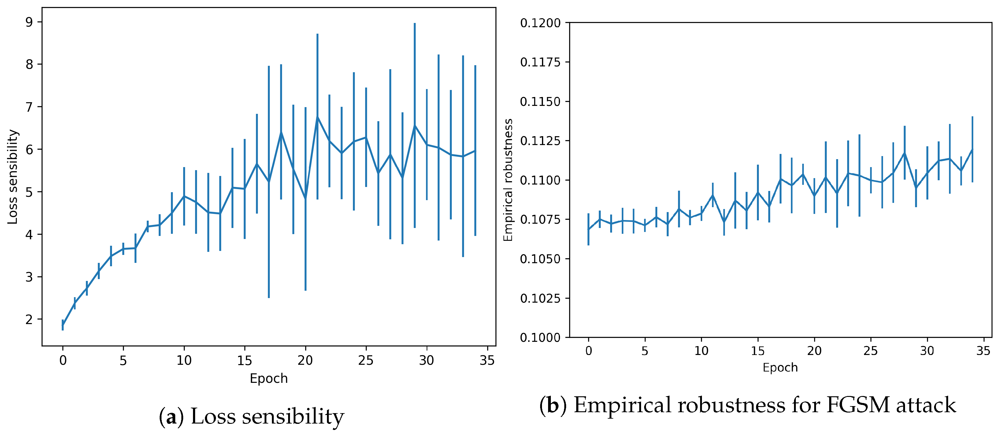
Regarding the other metrics (see Figure 10) Loss sensibility follows the same pattern with values that escalate from 0.6–1.4 to 2.0–9.0, measures that overfitting has been produced indeed.
Finally, Empirical robustness shows how the minimal perturbation needed to fool the model remains constant but with a tendency to increase its value throughout the epochs (in contrast to the no-overfitting regime).
4. Conclusions
In the first experiment, a training without overfitting is performed, so the model generalizes well on the validation set and, supposedly, on data from the test set and similar datasets. When a model is trained on this regime, we detect that adversarial robustness drops with the training epochs at the same time that test accuracy increases. However, the second experiment does not show this behaviour. With overfitting, the ASR remains stable at lower values and decreases when the training epochs make performance decrease on the test set.
With the experimentation performed in this work, opposite behaviours are observed for the overfitting and no overfitting regimes. The former remains stable to adversarial robustness, even reducing the possible radius of affecting perturbations. In consequence, robustness to adversarial examples is shown to increase (as opposed to test set accuracy). This is also evident from the metrics of adversarial robustness considered. In the latter case, test accuracy increases but adversarial robustness decreases, for which an exploding incidence of adversarials is confirmed, with a greater space of perturbations to be used for adversarial attack methods.
Our results support the notion that the phenomenon of adversarial examples seem to be linked to the well-known fitting-generalization trade-off.
Author Contributions
Funding acquisition, O.D. and G.B.; investigation, A.P.; methodology, A.P.; project administration, G.B.; supervision, O.D.; validation, G.B.; writing—original draft, A.P.; writing—review and editing, O.D. and G.B. All authors have read and agreed to the published version of the manuscript.
Funding
This work was partially funded by projects TIN2017-82113-C2-2-R by the Spanish Ministry of Economy and Business and SBPLY/17/180501/000543 by the Autonomous Government of Castilla-La Mancha; as well as the Postgraduate Grant FPU17/04758 from the Spanish Ministry of Science, Innovation, and Universities.
Conflicts of Interest
The authors declare no conflict of interest.
Abbreviations
The following abbreviations are used in this manuscript:
| AE | Adversarial Example |
| ASR | Adversarial Successful Rate |
| CIFAR | Canadian Institute For Advanced Research |
| CLEVER | Cross-Lipschitz Extreme Value for nEtwork Robustness |
| CW | Carlini & Wagner |
| FGSM | Fast Gradient Sign Method |
| MNIST | Modified National Institute of Standards and Technology |
| PGD | Projected Gradient Descent |
| STL | Self-Taught Learning |
References
- Szegedy, C.; Zaremba, W.; Sutskever, I.; Bruna, J.; Erhan, D.; Goodfellow, I.; Fergus, R. Intriguing properties of neural networks. arXiv 2013, arXiv:1312.6199. [Google Scholar]
- Carlini, N.; Wagner, D. Towards evaluating the robustness of neural networks. In Proceedings of the 2017 IEEE Symposium on Security and Privacy (SP), San Jose, CA, USA, 22–24 May 2017; pp. 39–57. [Google Scholar]
- Chen, P.Y.; Sharma, Y.; Zhang, H.; Yi, J.; Hsieh, C.J. EAD: Elastic-net attacks to deep neural networks via adversarial examples. In Proceedings of the Thirty-Second AAAI Conference on Artificial Intelligence, New Orleans, LA, USA, 2–7 February 2018. [Google Scholar]
- Madry, A.; Makelov, A.; Schmidt, L.; Tsipras, D.; Vladu, A. Towards deep learning models resistant to adversarial attacks. arXiv 2017, arXiv:1706.06083. [Google Scholar]
- Tramèr, F.; Kurakin, A.; Papernot, N.; Goodfellow, I.; Boneh, D.; McDaniel, P. Ensemble adversarial training: Attacks and defenses. arXiv 2017, arXiv:1705.07204. [Google Scholar]
- Song, Y.; Kim, T.; Nowozin, S.; Ermon, S.; Kushman, N. Pixeldefend: Leveraging generative models to understand and defend against adversarial examples. arXiv 2017, arXiv:1710.10766. [Google Scholar]
- Papernot, N.; McDaniel, P.; Wu, X.; Jha, S.; Swami, A. Distillation as a defense to adversarial perturbations against deep neural networks. In Proceedings of the 2016 IEEE Symposium on Security and Privacy (SP), San Jose, CA, USA, 23–25 May 2016; pp. 582–597. [Google Scholar]
- Arpit, D.; Jastrzebski, S.; Ballas, N.; Krueger, D.; Bengio, E.; Kanwal, M.S.; Maharaj, T.; Fischer, A.; Courville, A.; Bengio, Y.; et al. A closer look at memorization in deep networks. In Proceedings of the 34th International Conference on Machine Learning, Sydney, Australia, 6–11 August 2017; Volume 70, pp. 233–242. [Google Scholar]
- Goodfellow, I.J.; Shlens, J.; Szegedy, C. Explaining and harnessing adversarial examples. arXiv 2014, arXiv:1412.6572. [Google Scholar]
- Galloway, A.; Taylor, G.W.; Moussa, M. Predicting adversarial examples with high confidence. arXiv 2018, arXiv:1802.04457. [Google Scholar]
- Kubo, Y.; Trappenberg, T. Mitigating Overfitting Using Regularization to Defend Networks Against Adversarial Examples. In Proceedings of the Canadian Conference on Artificial Intelligence, Kingston, ON, Canada, 28–31 May 2019; Springer: Berlin/Heidelberg, Germany, 2019; pp. 400–405. [Google Scholar]
- Ilyas, A.; Santurkar, S.; Tsipras, D.; Engstrom, L.; Tran, B.; Madry, A. Adversarial examples are not bugs, they are features. arXiv 2019, arXiv:1905.02175. [Google Scholar]
- Deniz, O.; Vallez, N.; Bueno, G. Adversarial Examples are a Manifestation of the Fitting-Generalization Trade-off. In Proceedings of the International Work-Conference on Artificial Neural Networks, Gran Canaria, Spain, 12–14 June 2019; Springer: Berlin/Heidelberg, Germany, 2019; pp. 569–580. [Google Scholar]
- Su, D.; Zhang, H.; Chen, H.; Yi, J.; Chen, P.Y.; Gao, Y. Is Robustness the Cost of Accuracy?—A Comprehensive Study on the Robustness of 18 Deep Image Classification Models. In Proceedings of the European Conference on Computer Vision (ECCV), Munich, Germany, 8–14 September 2018; pp. 631–648. [Google Scholar]
- Bottou, L.; Cortes, C.; Denker, J.S.; Drucker, H.; Guyon, I.; Jackel, L.D.; Le Cun, Y.; Muller, U.A.; Säckinger, E.; Simard, P.; et al. Comparison of classifier methods: A case study in handwritten digit recognition. In Proceedings of the 12th IAPR International Conference on Pattern Recognition, Conference B: Computer Vision & Image Processing, Jerusalem, Israel, 9–13 October 1994; Volume 2, pp. 77–82. [Google Scholar]
- Yadav, C.; Bottou, L. Cold Case: The Lost MNIST Digits. In Advances in Neural Information Processing Systems (NIPS) 32; Curran Associates, Inc.: Red Hook, NY, USA, 2019. [Google Scholar]
- Xiao, H.; Rasul, K.; Vollgraf, R. Fashion-mnist: A novel image dataset for benchmarking machine learning algorithms. arXiv 2017, arXiv:1708.07747. [Google Scholar]
- Coates, A.; Ng, A.; Lee, H. An analysis of single-layer networks in unsupervised feature learning. In Proceedings of the Fourteenth International Conference on Artificial Intelligence and Statistics, Ft. Lauderdale, FL, USA, 11–13 April 2011; pp. 215–223. [Google Scholar]
- Deng, J.; Dong, W.; Socher, R.; Li, L.J.; Li, K.; Li, F.-F. Imagenet: A large-scale hierarchical image database. In Proceedings of the 2009 IEEE Conference on Computer Vision and Pattern Recognition, Miami Beach, FL, USA, 20–25 June 2009; pp. 248–255. [Google Scholar]
- Krizhevsky, A. Learning Multiple Layers of Features from Tiny Images; Technical Report; University of Toronto: Toronto, ON, Canada, 2009. [Google Scholar]
- Pedraza, A.; Deniz, O.; Bueno, G. Approaching Adversarial Example Classification with Chaos Theory. Entropy 2020, 22, 1201. [Google Scholar] [CrossRef] [PubMed]
- Kurakin, A.; Goodfellow, I.; Bengio, S. Adversarial examples in the physical world. arXiv 2016, arXiv:1607.02533. [Google Scholar]
- Moosavi-Dezfooli, S.M.; Fawzi, A.; Frossard, P. Deepfool: A simple and accurate method to fool deep neural networks. In Proceedings of the IEEE Conference on Computer Vision and Pattern Recognition, Las Vegas, NV, USA, 26 June–1 July 2016; pp. 2574–2582. [Google Scholar]
- Weng, T.W.; Zhang, H.; Chen, P.Y.; Yi, J.; Su, D.; Gao, Y.; Hsieh, C.J.; Daniel, L. Evaluating the robustness of neural networks: An extreme value theory approach. arXiv 2018, arXiv:1801.10578. [Google Scholar]
- LeCun, Y.; Bottou, L.; Bengio, Y.; Haffner, P. Gradient-based learning applied to document recognition. Proc. IEEE 1998, 86, 2278–2324. [Google Scholar] [CrossRef] [Green Version]
- Papernot, N.; McDaniel, P.; Goodfellow, I. Transferability in machine learning: From phenomena to black-box attacks using adversarial samples. arXiv 2016, arXiv:1605.07277. [Google Scholar]
Figure 1.
Adversarial example. From (left) to (right): original image (classified as “whistle”), adversarial noise added, resulting adversarial image (classified as “screw”).
Figure 1.
Adversarial example. From (left) to (right): original image (classified as “whistle”), adversarial noise added, resulting adversarial image (classified as “screw”).

Figure 2.
Samples from the datasets in this work.

Figure 3.
Training progress for normal training.

Figure 4.
Progression in the no-overfitting regime.

Figure 5.
CLEVER metrics without overfitting.

Figure 6.
Adversarial metrics in CIFAR-10 dataset without overfitting.

Figure 7.
Training curve for the overfitting regime. Notice that beyond epoch 6 the validation
accuracy tends to decrease while training accuracy keeps increasing.
Figure 7.
Training curve for the overfitting regime. Notice that beyond epoch 6 the validation
accuracy tends to decrease while training accuracy keeps increasing.

Figure 8.
Attack Success Rate vs Test Accuracy in overfitting regime.

Figure 9.
CLEVER metrics with overfitting.

Figure 10.
Adversarial metrics in CIFAR-10 dataset with overfitting.


Table 1.
Distance metrics derived from the norm.
| Norm | Calculation | Explanation |
|---|---|---|
| non-zero elements | number of perturbed pixels | |
| Euclidean distance | distance in the image space | |
| largest value | highest perturbation at any pixel |
Table 2.
Average distances for the adversarial sets without overfitting for CIFAR-10.
| Method | |||
|---|---|---|---|
| CW | 1024.00 ± 0.00 | 0.43 ± 0.48 | 0.07 ± 0.06 |
| FGSM | 1017.92 ± 25.30 | 8.93 ± 0.48 | 0.30 ± 0.00 |
| PGD | 1018.99 ± 20.87 | 8.10 ± 0.57 | 0.30 ± 0.00 |
Table 3.
Average distances for the adversarial sets without overfitting for STL-10.
| Method | |||
|---|---|---|---|
| CW | 9216.00 ± 0.00 | 0.97 ± 1.42 | 0.06 ± 0.06 |
| FGSM | 8969.59 ± 387.89 | 26.41 ± 1.39 | 0.30 ± 0.00 |
| PGD | 9049.55 ± 262.61 | 23.37 ± 1.17 | 0.30 ± 0.00 |
Table 4.
Average distances for the adversarial sets with overfitting for CIFAR-10.
| Method | |||
|---|---|---|---|
| CW | 1024.00 ± 0.00 | 0.49 ± 1.15 | 0.06 ± 0.08 |
| FGSM | 1017.19 ± 27.86 | 8.64 ± 0.52 | 0.30 ± 0.00 |
| PGD | 1019.08 ± 20.05 | 7.62 ± 0.45 | 0.30 ± 0.00 |
Table 5.
Average distance metric for the adversarial dataset with overfitting for STL-10.
| Method | |||
|---|---|---|---|
| CW | 9216.00 ± 0.00 | 0.82 ± 2.37 | 0.06 ± 0.07 |
| FGSM | 8951.35 ± 408.80 | 26.04 ± 1.47 | 0.30 ± 0.00 |
| PGD | 9021.16 ± 289.93 | 23.32 ± 1.29 | 0.30 ± 0.00 |
Publisher’s Note: MDPI stays neutral with regard to jurisdictional claims in published maps and institutional affiliations. |
© 2021 by the authors. Licensee MDPI, Basel, Switzerland. This article is an open access article distributed under the terms and conditions of the Creative Commons Attribution (CC BY) license (https://creativecommons.org/licenses/by/4.0/).
Share and Cite
MDPI and ACS Style
Pedraza, A.; Deniz, O.; Bueno, G. On the Relationship between Generalization and Robustness to Adversarial Examples. Symmetry 2021, 13, 817. https://doi.org/10.3390/sym13050817
AMA Style
Pedraza A, Deniz O, Bueno G. On the Relationship between Generalization and Robustness to Adversarial Examples. Symmetry. 2021; 13(5):817. https://doi.org/10.3390/sym13050817
Chicago/Turabian StylePedraza, Anibal, Oscar Deniz, and Gloria Bueno. 2021. "On the Relationship between Generalization and Robustness to Adversarial Examples" Symmetry 13, no. 5: 817. https://doi.org/10.3390/sym13050817
Note that from the first issue of 2016, this journal uses article numbers instead of page numbers. See further details here.