
Accessing Imbalance Learning Using Dynamic Selection Approach in Water Quality Anomaly Detection


1
Department of Electrical and Electronic Engineering Science, University of Johannesburg, Auckland Park, Johannesburg 2006, South Africa
2
Faculty of Engineering and the Built Environment, Durban University of Technology, Durban 4000, South Africa
3
Sustainable Human Settlement and Construction Research Centre, Faculty of Engineering and the Built Environment, University of Johannesburg, Auckland Park, Johannesburg 2006, South Africa
*
Author to whom correspondence should be addressed.
Symmetry 2021, 13(5), 818; https://doi.org/10.3390/sym13050818
Submission received: 17 February 2021
/
Revised: 26 March 2021
/
Accepted: 1 April 2021
/
Published: 7 May 2021
(This article belongs to the Section Computer)
Abstract
:Automatic anomaly detection monitoring plays a vital role in water utilities’ distribution systems to reduce the risk posed by unclean water to consumers. One of the major problems with anomaly detection is imbalanced datasets. Dynamic selection techniques combined with ensemble models have proven to be effective for imbalanced datasets classification tasks. In this paper, water quality anomaly detection is formulated as a classification problem in the presences of class imbalance. To tackle this problem, considering the asymmetry dataset distribution between the majority and minority classes, the performance of sixteen previously proposed single and static ensemble classification methods embedded with resampling strategies are first optimised and compared. After that, six dynamic selection techniques, namely, Modified Class Rank (Rank), Local Class Accuracy (LCA), Overall-Local Accuracy (OLA), K-Nearest Oracles Eliminate (KNORA-E), K-Nearest Oracles Union (KNORA-U) and Meta-Learning for Dynamic Ensemble Selection (META-DES) in combination with homogeneous and heterogeneous ensemble models and three SMOTE-based resampling algorithms (SMOTE, SMOTE+ENN and SMOTE+Tomek Links), and one missing data method (missForest) are proposed and evaluated. A binary real-world drinking-water quality anomaly detection dataset is utilised to evaluate the models. The experimental results obtained reveal all the models benefitting from the combined optimisation of both the classifiers and resampling methods. Considering the three performance measures (balanced accuracy, F-score and G-mean), the result also shows that the dynamic classifier selection (DCS) techniques, in particular, the missForest+SMOTE+RANK and missForest+SMOTE+OLA models based on homogeneous ensemble-bagging with decision tree as the base classifier, exhibited better performances in terms of balanced accuracy and G-mean, while the Bg+mF+SMENN+LCA model based on homogeneous ensemble-bagging with random forest has a better overall F1-measure in comparison to the other models.
1. Introduction
Access to clean and safe drinking water is vital to human life. It is therefore imperative that water is suitable for drinking and other uses. Most medical-related experts agree that most public health epidemics have their source in poor water quality. These are categorised into four: waterborne, water-based, water-related and water-scarce diseases [1]. Therefore, water of good quality and easy access must be provided to the public as it leads to a reduced burden on health care facilities, which directly impacts the economy and national security of nations [2].
Furthermore, in today’s volatile socio-political atmosphere, water quality anomaly event detection has become critical to national security and public health [2], hence there is a greater need to detect anomalies, deter and prevent both intentional and unintentional sabotage that may compromise the water quality distribution systems [3]. Owing to the massive amount of data currently generated by water utilities and the water industry’s impact on citizens’ lives, there is a need to implement better water quality monitoring and prediction methods based on new and advanced technologies, specifically for this study, new and effective machine learning, and data mining techniques [4]. Anomaly detection in drinking-water quality is a classification problem that seeks to predict a minority class of interest of an event in an imbalanced class distribution scenario with an overwhelming number of the majority class examples. The challenge of learning in the presence of imbalanced data is further complicated if the dataset has missing data or noise. The existence of missing data is a common occurrence in either wireless sensor-generated data caused by faulty measuring sensors or data corrupted in transit. In this study, our aim is the optimisation of learning algorithms for imbalanced class distribution in the water quality anomaly detection (WQAD) classification problem. Imbalance class distribution and missing values in data are prevalent and challenging problems in numerous domains, including in WQAD, resulting in performance degradation when using traditional machine learning algorithms. This is because these traditional learning algorithms assume completeness of data and balanced class distribution. In recent times, numerous machine learning methods have been proposed in literature ranging from single classifiers, such as support vector machine (SVM), Logistic Regression, and bagging or boosting ensemble approaches, combined with resampling and cost-sensitive preprocessing methods [5].
Dynamic selection systems have recently gained considerable research attention due to their better performance and advantage in learning imbalance data, especially for small-sized or ill-defined datasets classification tasks, compared to the traditional single machine learning and static ensemble selection systems [6]. The two dynamic selection approaches in Multiple Classifier Systems (MCS) research realms are the Dynamic Classifier Selection (DCS), which selects the most competent single classifier, and the Dynamic Ensemble Selection (DES), which selects the most optimal ensemble of classifiers to predict each test sample [7,8]. Dynamic selection (DS) refers to a process where the base classifier or estimator, usually a single classifier belonging to a pool of classifiers, is selected dynamically to predict the new specific test sample’s label to be classified [9]. The composition of DS changes each time new and different test examples are introduced to the system for prediction or classification. This is based on the intuition that in a pool of classifiers, each base classifier has its competence in classifying new unknown test samples for the different local region of competence according to certain selection criteria such as accuracy or ranking in the given feature space. A base classifier is a term that refers to a single classifier belonging to an ensemble or a pool of classifiers [10].
As reported in [8], the majority of DS systems are heavily dependent on the k-Nearest Neighbor (k-NN) algorithm that is necessary for defining the region of competence (RoC). This limits the performance of these DS methods on improving the k-NN algorithm during the RoC definition. Nevertheless, the DS approaches are reported in the research literature to improve the performance of traditional static boosting and bagging-based methods. This has informed the rise of researchers employing DS techniques combined with ensemble-based approaches [9,11]. For the imbalanced dataset problem, there is a consensus in several research papers that noise and the degree of class overlapping are the main culprits in performance degradation in learning classifiers, as against purely class imbalance. In nearly all DS strategies, k-NN is used in estimating the competence of base classifier in RoC using a set of labelled instances referred to as DSEL. Meanwhile, Wilson’s Edited Nearest Neighbor (ENN) technique [12] is reported in the literature to considerably improve the performance of the k-NN algorithm [8,13].
Furthermore, while most DS techniques use only one selection criterion for measuring the competence level (expertise) of base classifiers, this has a limiting performance effect on the DS schemes in estimating the level of competence of base classifiers and, by extension, affecting the overall performance of DS methods. This is because of the probability of not selecting the most competent base classifier for a test instance in a given classification problem using a single competency selection criterion. Contrary, as an exception, to the DS methods that use single competency selection criteria is the newly proposed Meta-learning for Dynamic Ensemble Selection (META-DES) technique that uses several different criteria to estimate the competence level of base classifiers, thus increasing the likelihood of improving the classification performance in DES. More so, META-DES and its variants are reported in the literature to outperform other DS techniques evaluated in numerous scenarios [10]. The idea fronted in this paper is that the hybrid SMOTE+Edited Nearest Neighbor (SMOTE+ENN) data resampling method at the pool generation stage could indirectly mitigate ambiguity to the learning classifier by removing noisy and class overlapping instances for a clear-cut decision boundary and passed onto the DSEL for an improved DS selection phase. At the same time, the multiple criteria provided by the META-DES algorithm for estimating the base classifier’s competence level would most likely improve classification performance. Hence, the advantages that the combined SMOTE+ENN with META-DES method bring give us a reason that it would lead to improved performance of DS schemes. The experimental outcome is observed in Section 4 compared to the SMOTE and SMOTE+Tomek’s Links (SMOTE+TL) resampling methods.
Symmetry is a concept embedded in many physical and biological objects in the environment. Hence, to improve the predictive performance of learning algorithms in the presence of imbalanced datasets with missing values, incorporating, adapting and building symmetry in machine learning and artificial intelligence in pattern recognition tasks is currently emerging as an important research niche because of the proven advantages it provides. Specifically, the concept of symmetry-adapted machine learning in water quality anomaly detection transforms data to extract and analyse hidden patterns to enable the detection of new anomalies. Which, in general, mitigates complexity in data processing, reduces the training and future detection times.
Our experimental investigation is, therefore, the combination of one missing data method, three SMOTE-based resampling methods (SMOTE, SMOTE+ENN and SMOTE+TL) combined with six DS techniques using bagging-based ensemble with either decision tree or random tree as the base classifiers, in addition to experimenting using the heterogeneous voting classifier approach. This allows us to comprehensively observe the behaviour of the combination of these methods on the WQAD dataset. This study extends the earlier work in [14] and largely inspired by the other promising results obtained in [6], [11] using DS techniques on several relatively smaller benchmark imbalanced datasets. The conclusion drawn from the research study in [9] suggested a link between DS techniques’ performance and the inherent aspects of the classification difficulty related to the data complexity. This finding motivates this study to empirically investigate the suitability of DS for the current WQAD dataset classification problem from the perspective of data complexity measure.
To this end, the following research questions are posed:
- What is the level of classification complexity of the imbalanced WQAD dataset in comparison to other imbalanced datasets?
- Are dynamic selection approaches suitable for imbalanced WQAD classification task?
- Do dynamic selection techniques improve the classification performance of the WQAD dataset problem in comparison to static classifiers or static ensemble methods, or both?
Consequently, this study’s hypothesis is formulated that it is possible to improve the performance of ensemble-based approaches on imbalanced WQAD classification problems using dynamic selection techniques combined with missing data and resampling methods. Hence, the following highlights the contributions of this study:
- To investigate several solutions for the classification of imbalanced real-world drinking-water quality anomaly detection task.
- To analyse the complexity of a large WQAD dataset and the suitability of applying dynamic selection approaches to this dataset.
- To improve and evaluate the performances of six dynamic selection techniques combined with ensemble learning models and one missing data, and three SMOTE-based resampling approaches to tackle the WQAD problem.
The rest of the paper is organised as follows: Section 2 provides an overview of this study’s main concepts and related works. Section 3 describes the experimental research approach and framework. The experimental results, discussions on key findings, and statistical test and comparison of models are presented in Section 4. Section 5 presents a conclusion on the study, while Section 6 highlights the limitations and future research directions of this study.
2. Literature Review
2.1. Overview of Background Concepts
This paper is comprised of five main concepts: (1) Data imputation, (2) Imbalance learning, (3) Generation of the pool of classifiers, (4) Dynamic selection of classifiers, and (5) Data complexity measures. This section presents an overview of these key concepts and related works in WQAD tasks.
2.1.1. Data Imputation Method
A missing data method is a form of data cleaning technique for handling incomplete values or records or observations, usually anticipated to be in a dataset with some estimated values, rather than leaving them empty. Various strategies for handling missing data have been proposed in the literature; they include using statistical, machine learning, model-based using maximum likelihood with expectation-maximisation, and ensemble approaches [15]. Missing data strategies are broadly categorised into four: (1) Case deletion (filling with a suitable value, or ignoring data with missing data, or deleting or dropping missing data); (2) imputation strategies (mean, median, multiple imputation and machine learning such as k-NN; (3) model-based imputation strategies (maximum-likelihood with EM algorithm); and (4) machine learning-based strategies (ensemble and tree-based approaches) [15]. The presence of missing data in an imbalanced dataset adds complexity to the classification problem; hence, the need to be addressed during the data preprocessing phase. The non-parametric random forest-based imputation method (missForest) is considered in this study for handling missing data. The consideration is based on results obtained in the recent work in [14].
2.1.2. Imbalance Learning
In this study, the WQAD task is formulated as an imbalanced class distribution problem. This is because of the occurrence of the minority class that is poorly represented in the data space compared to the majority class representing the class of interest. The resampling methods aim to transform the dataset distribution to address the class labels’ imbalanced nature and mitigate its effect during the learning process [16]. Methods for dealing with class imbalance problems are broadly categorised into four [5,17]:
- Data level method: This method addresses the class imbalance problem by modifying the class distribution during preprocessing. Techniques that performs these class modifications are collectively referred to as resampling algorithms. The resampling techniques are broadly categorised into four: (1) over-sampling the minority class, (2) under-sampling the majority class, (3) hybrid combination of under-sampling used in conjunction with over-sampling methods and (4) ensemble-based approach [16].
- Algorithm level method: This approach adapts learning algorithms to handle the class imbalance distribution. The approach is achieved by internally modifying the learning algorithms to handle such a problem.
- Cost-sensitive method: This approach considers the misclassification cost associated with the minority and majority class instances in an algorithm’s learning process. For instance, because the minority class is usually the class of interest, a high misclassification cost is assigned to the minority class during the learning process to underscore its importance, thereby weakening in the process the majority class.
- Ensemble-based methods: This approach combines data-level, cost-sensitive or algorithm-level approaches during preprocessing using an ensemble-based learning algorithm.
SMOTE [18] and two of its hybrid variants: SMOTE+TL and SMOTE+ENN [19] are the selected resampling methods investigated in this work. In the first, SMOTE oversamples the minority class by creating new synthetic minority class instances through interpolating between several of these instances laying together; Tomek link cleans the SMOTE over-sampled training set by removing both the majority and minority class instances that form Tomek links and that are considered as noise or borderline instances from the already balanced dataset. SMOTE+ENN is similar to SMOTE+TL, where SMOTE also balances the dataset by oversampling the minority class, then followed by the data cleaning process performed by Wilson’s Edited Nearest Neighbor Rule (ENN) [12]. The ENN removes any instances of either the majority or minority class that differs from at least two of its three nearest neighbors. In both approaches, the aim is to provide a better-defined decision boundary and class clusters by removing data instances deem to be noise or in the overlapping region, thereby minimising learning ambiguity for the classifier. Generally, as shown in literature, SMOTE+ENN does a deeper cleaning than SMOTE+Tomek, hence is normally expected to provide a better well-defined class cluster than SMOTE+TL [19] in most dataset problems. Therefore, the choice of the two resampling techniques is considered based on the assertion in several research papers that noise and the degree of class overlapping are the main culprits in performance degradation in learning classifiers, as against purely class imbalance. Moreover, all the DS techniques investigated in this study use k-NN for the competence of region definition, and the ENN technique is reported in the literature to improve the performance of the k-NN [13] considerably. SMOTE technique is included in the evaluation to serve as a baseline for the other two hybrid variants.
2.1.3. Pool Generation of Classifiers
A Multiple Classifier System (MCS) comprises three phases: pool generation, selection, and integration, as shown in Figure 1. The pool generation phase 1 involves generating a pool of diverse and accurate classifiers. The pool diversity is achieved through either a homogeneous ensemble pool using either bagging, boosting or hybrid schemes or a heterogeneous ensemble pool of different base classifiers [9]. In the selection phase (phase 2), a single or a set of multiple classifiers from the pool is selected. In the final phase 3, the selected classifier (DCS) or classifiers (DES) predictions are integrated for the final decision. In certain scenarios, such as when the whole classifier pool in phase 1 is used, the selection phase becomes unnecessary. When just a single classifier is selected, the integration phase, this time around, becomes unnecessary. A static ensemble approach is usually used to integrate the final decision of the generated pool of classifiers [9]. This paper focuses on phase 1 and 2, on homogeneous and heterogeneous pool generation schemes and the DS strategies.
2.1.4. Dynamic Selection
Dynamic selection (DS) is a technique given a test example that allows the selection of a single or more than one base classifiers from a pool using their competency levels (expert or best classifier) and a competence measure to form the ensemble [11]. This is based on the intuition that each base classifier is an expert for the different local region in the feature search space. DS’s goal is to determine a group of classifiers in a pool having the best classifiers for a classification problem when presented with different test instances. On the contrary, in a static ensemble, all the base classifiers are pooled together each time during the training phase for a given test example regardless of each base classifier’s competence. Theoretical and empirical research studies have shown dynamic selection improved performance over static selection strategies [20]. In DS, a three-step process helps in defining the specific ensemble of classifiers (EoC); they are (1) definition of region of competence, (2) competence of classifiers estimation and (3) the classifier(s) selection approach. This paper favours the ensemble-bagging pool generation approach due to its popularity and following on the recent work by [10]. This current study combines data imputation and resampling methods with a dynamic selection approach. Dynamic selection strategies are grouped into dynamic classifier selection (DCS) and dynamic ensemble selection (DES).
DCS selects a single classifier during the pool generation phase, while the DES approach selects an ensemble of classifiers based on their competence to classify a test instance. In this study, three DCS strategies, namely Modified Classifier Rank (Rank), which measure the competence of classifiers based on ranking, Local Class Accuracy (LCA) and Overall Local Accuracy (OLA), both measures the competence of classifier using on accuracy in the local region of the feature space, are considered [9]. For DES techniques, two k-nearest oracle information-based strategies, namely KNORA-Eliminate (KNORA-E) and KNORA-Union (KNORA-U) [21], and one meta-classifier strategy (META-DES) [10] are considered. Both KNORA-E and KNORA-U are Oracle-based methods, as the methods use the concept of linear random oracle [22], while META-DES uses meta-classifier as a competency estimator. The summary of the six dynamic selection strategies is listed in Table 1. The techniques are selected based on their reported improved performances from studies in [9,10,11,23].
The six strategies are briefly described as obtained from [9,24]. Figure 2 depicts the three steps in the DS approach. The dynamic selection dataset (DSEL) is either the training or validation set, while is the query examples that are used to defines the region of competence (RoC) of query example. C is the pool of classifiers with M size, δ is the vector that estimates competences of each base classifier in C. is the final EoC, depending on the DS strategy of either one base classifier in DCS or more than one base classifiers in DEC schemes. The vector δ is used to define EoC that will be used to label query examples .
- Modified Class Rank (Rank) [9,25] is a method that is based on the ranks of individual classifiers in the pool for any particle test instance. The classifier’s rank is an estimated measure of its local accuracy assigned to a class label by a classifier within a neighbourhood of each test instance, which has been correctly labelled. The classifier with the highest local accuracy is the highest-ranked and the most competent, and is thus selected for the classification problem.
- Local Class Accuracy (LCA) [9,25] is a strategy that estimates each classifier’s accuracy in a local region within a given test instance concerning some output class. The classifier that predicts the correct class label in the local region is adjourned most competent and is selected to classify the test instance.
- In Overall Local Accuracy (OLA) strategy [9,25], selects the most competent base classifier using the calculated accuracy in the entire RoC as the competence level criterion measure, with the classifier obtaining the highest accuracy selected as the most competent classifier for the given test instance. Rank works similarly to OLA. The only difference is that weight is assigned to each instance belonging to the region of competence with the Euclidean distance to the query instance.
The dynamic ensemble selection (DES) method selects from a pool of classifiers an ensemble of classifiers based on their competence to classify a test instance. The competence level of classifiers is estimated over each test instance’s nearest neighbors, based on certain criterion. The two DS techniques are briefly described as follows:
- KNORA-E [9,21] considers and selects a competent classifier based on the oracle concept if the classifier attains a perfect accuracy for all test instances over the whole region of competence. Only the classifiers that attain an excellent accuracy are finally selected and combined using a voting system. It is possible not to have a classifier that attains a perfect accuracy; in that case, the RoC is reduced, and the process of selection repeated by re-evaluating the classifiers.
- KNORA-U [9,21] method measures the level of competence of a base classifier based on the number of correctly classified instances in the defined region of competence. In KNORA-U, every classifier that classifies at least one instance correctly belonging to the query instance in the Roc has a voting right. The votes obtained by each selected base classifier, which is equal to the correctly predicted labels in the RoC, are combined to form the final ensemble.
- META-DES [10] is a framework that formulates the dynamic ensemble selection problem as a meta-problem, whereby a meta-classifier works as a classifier selector. The algorithm uses a set of multiple different criteria regarding the base classifier’s , behaviour (as against a single criterion) to determine whether is competent enough or not, to label the query test sample . The META-DES is defined in the following steps:
Step 1: The meta-classes are either competent–1 or incompetent 0 to classify .
Step 2: Each set of meta-features fi corresponds to multiple criteria for measuring a base classifier’s level of competence, which are measures of different characteristics behaviour about the base classifier.
Step 3: The meta-features are encoded into a meta-features vector
Step 4: A meta-classifier is trained based on the meta-features to estimate whether or not will achieve the correct prediction . In other words, it determines if the is competent enough to classify the test sample query . In the end, the competent classifiers are selected from the pool for performing the classification using a majority voting mechanism.
2.1.5. Data Complexity Measure
Dynamic selection methods’ choice and performance are attributable to the dataset classification problem’s complexity [9]. The complexity measures define three characteristics of the dataset, namely, geometric and topology, class overlapping of individual feature values and boundary distributions between classes [26]. Furthermore, the study in [9] concludes that more than just the dataset sample size, its number of features and classes; the inherent and unique characteristic of a dataset play a more crucial role in the performance of dynamic selection methods in relationship with the dataset complexity. Meanwhile, the authors in [27] argue that data complexity has a performance impact on optimising class-imbalanced classification problems when using combined resampling and learning classifier. Considering all these arguments, this paper is inspired to assess the complexity of the WQAD dataset used in this study and the appropriateness and suitability of applying the dynamic selection (DS) approach to this dataset. The dataset’s complexity is evaluated by analysing eight different complexity measures for the imbalance binary classification problem previously examined in these two studies [26,28]. As also pointed out in [26,28], combining these eight different measures would more likely provide insightful information regarding our dataset’s complexity. The nine complexity measures are six feature-based measures (Maximum Fisher’s Discriminant Ratio (F1), the Directional-vector Maximum Fisher’s Discriminant Ratio (F1v), Volume of Overlapping Region (F2), Maximum Individual Feature Efficiency (F3), Collective Feature Efficiency (F4) and Average number of features per dimension (T2)); one neighbourhood-based measure (the error rate of 1NN classifier (N3)); and two dimensionality-based measures, (Average number of PCA dimensions per points (T3) and Ratio of the PCA Dimension to the Original Dimension (T4)). These classification complexity measures are briefly described next as obtained in [26,28].
- Maximum Fisher’s Discriminant Ratio (F1) is a measure that computes the overlap between feature values and the different classes, and it is defined in Equation (1) as:where, are the means, and are the variances of class1 (True) and class2 (False) in that feature dimension. A high F1 value indicates a weak overlap between classes and represents a lower complexity and easier classification problem. F1 is in the range of [≈0 to 1].
- The Directional-vector Maximum Fisher’s Discriminant Ratio (F1v) is a measure that complements F1 by considering a directional Fisher criterion and is defined as given in Equation (2):where, directional Fisher criterion is given as , d is the directional vector that allows for maximum class separation, B is the scatter matrix between-class, and W is a scatter matrix within-class. A lower F1v score indicates a simpler classification problem.
- The volume of Overlapping Region (F2) computes the range of normalised minimum and maximum overlapping intervals of distribution of features values within classes. F2 is defined as in Equation (3):F2 may yield a negative value for non-overlapping feature ranges. The lower the F2 value, the lower the classes’ overlap, indicating a less complex classification problem.
- Maximum Individual Feature Efficiency (F3) estimates each feature’s individualised efficiency in separate classes. F3 is express as given in Equation (4) for features:where, computes the number of examples in the region of overlap for feature, while is indicator function (). The values are the maximum and minimum values of each feature in a class , respectively. A low value of F3 indicates a non-complex classification problem.
- Collective Feature Efficiency (F4) is a measure that gives insight into how the features interact together by considering and selecting features one after another, which shows a lesser overlap between classes via a process through the entire dataset. After that, F4 computes the ratio of examples that remained and overlapped between classes. F4 is expressed as in Equation (5):where, compute the number of points in the overlapping region of the feature for the dataset from the round . Lower values of F4 indicate a non-complex classification problem.
- The error rate of the 1NN classifier (N3) computes the estimated error rate of the k-nearest neighbour classifier based on the proximity of the opposite classes’ points using a Leave-One-Out (L-O-O) cross-validation estimation scheme. N3 is defined as in Equation (6):where, is the k-nearest neighbour classifier’s prediction for a test instance , using all the other instances as the training set and repeated n times with n different training set and n different test set, where n is the total number of instances in the dataset.However, because of our WQAD dataset’s size, its imbalanced class distribution, and the associated computational cost of using L-O-O scheme on a large dataset, an equivalent estimate of N3 using 10-fold stratified cross-validation (CV) is instead computed relying on the empirical evidence in [29]. Moreover, in stratified CV, each fold has approximately the same proportion of class labels leading to a relatively better bias and variance. A lower N3 value suggests an easier classification problem, based on the indication that many instances are far from instances of other classes. N3 is in the range of [0 to 1].
- The average number of features per dimension (T2) is a measure that divides the number of instances (n) in the dataset by the number of features (m) representing their dimensionality. T2 takes an inverse form and is expressed as in Equation (7):T2 can assume arbitrarily large or small values and sometimes even takes negative values when the number of instances is highly more than the number of features in a dataset. Higher T2 indicates an easier classification problem.
- The average number of PCA dimensions per points (T3) assess data sparsity and is the principal component analysis (PCA) of the dataset representing the number of PCA components covering 95% of the data variability . Smaller values of T3 indicates a simpler classification problem. T3 is defined in Equation (8) as:
- The ratio of the PCA Dimension to the Original Dimension (T4) indicates an approximate estimate of the proportion of relevant dimension of the dataset, measured based on PCA criterion. A smaller T4 value indicates a less complex problem. T4 is expressed in Equation (9) as:
2.2. Related Works
Several works on WQAD using machine learning and statistical analysis approaches have been published over the years, as captured in the review work in [4]. However, this paper will focus mostly on contributions of a few recently published works in an industrial competition for drinking-water quality anomaly detection [30], utilising the same real-world drinking-water quality anomaly detection dataset examined in this current study. This approach ensures a fair comparison.
A study using various tree-based ensemble approaches is investigated in [31]; the study observed that the gradient boosting methods are more particularly able to overcome imbalanced time series data and multicollinearity with satisfactory predictive performance. Several machine learning and deep learning models to deal with anomaly in water quality based on time series data are examined, namely, logistic regression (LR), linear discriminant analysis, SVMs, artificial neural network (ANN), deep neural network (DNN), recurrent neural network (RNN) and long short-term memory (LSTM). In comparison to the LR model, SVM exhibits better performance and SVM, ANN and LR are less susceptible to the imbalanced dataset when compared to the DNN, RNN and LSTM deep learning models [32]. Multi-objective machine learning optimisation is used for feature selection, and ensemble generation is proposed in [33] to solve online anomaly detection of drinking-water quality based on time series. When tested on the validation test set, the proposed model could generalise well on future test set predictions. Furthermore, two ensemble learning models for dealing with imbalanced dataset are proposed, namely SMOTEBoost and RUSBoost using oversampling and undersampling techniques [34]. Finally, multi-objective pruning on the base models for the ensembles applied to optimise the prediction and generalisation performance. In a recent related and relevant study, two models are proposed: adaptive learning rate backpropagation (BP) neural network (ALBP) and 2-step isolation and random forest (2sIRF), to predict water quality based on physical and biological indicators in an urban water supply scenario [35]. Their result shows that 2sIRF showed a higher prediction accuracy and considers the risk distribution within the supply system. In a latest similar work, the study proposed a RUSBoost-based dynamic multi-criteria ensemble selection mechanism, considering to better cope with the trade-off between false positives, which would lead to financial losses to water utilities, and false negatives, which would have critical and negative implications to public health, national security and the environment in drinking-water quality anomaly detection monitoring systems [23]. The study reports a 15% improvement of the proposed model over other ensemble learning and dynamic selection methods in terms of F1-scores.
It is noticed that most of these works focused on specific missing data and imbalanced class methods in dealing with the challenges in this domain. In most of these works, the models’ evaluation is mainly based on the balanced training or validation test, since as a rule, the preprocessing methods are only applied to the training set. However, the models’ performance results obtained on the imbalanced test set (unseen dataset) are usually different from those obtained based on the balanced training set.
In notable recent related works in imbalanced classification using DS, five variants of resampling methods, namely, SMOTE, Random Balance and Random Minority Oversampling (RAMO) techniques in combination with four DS methods (RANK, LCA, KNORA-U and KNORA-E) across several imbalanced dataset problems are considered [11], with dynamic ensemble reported to improving the F-measure and G-mean and higher ranks considering different levels of imbalance in comparison with the other static ensemble methods. Similarly, the effectiveness of DS strategies for imbalance classification task has also been investigated in [8,9,10] across several benchmark datasets. However, all these studies used relatively smaller dataset sizes (instances) than the WQAD dataset used in this paper.
The majority of recent works in WQAD apply modifications to non-ensemble and ensemble classifiers in combination with resampling methods as the widely adopted approach. Although it has been demonstrated that DS approaches are effective for imbalanced classification, the performance by coupling of missing data and class imbalance methods with dynamic selection techniques to the best of our knowledge has been rarely considered or explored in the WQAD domain problem with a relatively larger dataset, as inferred in the studies in [6]. Besides this, no study extensively investigates the suitability of DS approaches to real-world WQAD problem, except in [23], where the authors’ proposed a RUSBoost-based DES mechanism to address balancing multiple conflicting criteria to achieve a better trade-off between false positives and false negatives in two-class classification problems. The proposed model was then compared to other DS methods.
3. Materials and Methods
This section presents the experimental setup followed in this study. The different experiments conducted and the framework used is first outlined. Then a summary is given of the main dataset characteristics, the hyperparameter tuning of the methods investigated and the performance measures evaluated.
3.1. Experimental Setup
The experiments were performed in a Python environment using DESLib-Dynamic Ensemble Learning Library in Python [20] and other sci-kit-learn libraries. This paper aims to combine missing data and resampling methods with dynamic selection approaches to observe the effects this combination has on anomaly detection in the drinking-water quality classification problem. The MV and resampling methods considered in this paper were selected based on an earlier study in [14]. Firstly, sixteen most used state-of-art non-ensemble and static ensemble algorithms in the WQAD research domain are considered and optimised to investigate if their performances could be improved. This experiment is reported as experiment 1, and their results are reported in Section 4.
The three resampling methods were optimised based on the hyperparameters tuning using grid-search strategy.
Table 2 summarises all the ensemble-based models evaluated in this study. They comprise a combination of one missing data (missForest), three resampling methods (SMOTE, SMOTE+ENN and SMOTE+TL) and six dynamic selection, considering homogenous and heterogeneous ensemble schemes. For the homogeneous ensemble scheme, the bagging-based method is used, while for the heterogeneous ensemble scheme, the voting classifier is used. Two optimised base classifiers were investigated for the homogeneous ensemble experiments, namely decision tree and random forest reported in experiment 2. For experiment 2, two scenarios are considered. First, a combination of the optimised pool of base classifiers and the resampling methods using the default settings. In the second scenario, combining the optimised pool of base classifiers and the optimised resampling methods was considered. The parameter settings for the resampling and dynamic selection methods are adopted from the studies in [11,24]. Meanwhile for the heterogeneous ensemble, the scheme was composed of three different optimised pools of classifiers, namely k-NN, random forest and decision tree reported in experiment 3.
The pool size for all homogeneous ensemble schemes was set at 100. A further test by increasing the pool size to 200 for the two base estimators did not improve the learning performance. The three resampling methods were optimised based on the hyperparameters as listed in Section 3. Lastly, for all the DS methods, the k-nearest neighbours’ parameter was set to k = 7 (the default configuration). The k parameter value is used in defining the size of the region of competence, which influences the overall performance of DS strategies. Even though three other k-nearest neighbours’ values (k = 3, 5 and 9) were tested, it did not yield improved performance.
For the missing data method and each of the three resampling methods, 39 variations of models were produced, composed of six ensemble-based dynamic selection strategies. For example, Bg+mF+SMENN+META is the combined variant of miss Forest, SMOTE+ENN resampling and META-DES DS methods using bagging based ensemble, while Vg+mF+SMTL+META is the combined variant of missForest, SMOTE+TL resampling and META-DES DS methods in a heterogeneous based ensemble using voting classifier scheme. All the ensemble-based models used in this study are described in Table 2. Five performance measures were used to evaluate the models’ performances, namely, balanced accuracy, precision, recall, F-measure and G-mean. Figure 3 shows the experimental framework used in training and testing the DS models investigated in this paper, similar to the framework used in [11]. The approach in Figure 3 involves applying the preprocessing techniques: data normalisation to rescale each feature into a range of [0,1] on the training and tests to avoid dominance of one feature over another, and (missing data and resampling methods) on the training set only. The modified (resampled) dataset is used to train the ensemble (homogeneous and heterogeneous) and the DS approach, in addition to generating the DSEL. The preprocessed training set was split into two halves, one-half for training the base classifiers and the other half DSEL for DS. This decision was possible since there was enough training dataset size. The randomised characteristics introduced by the preprocessing methods into the DSEL ensured it was different from the training set, hence avoiding possible data leak that would lead to overfitting. During testing, the DS methods used the DSEL to derive the RoC for a given test instance, and then the set-aside test data is used to evaluate the selected DS strategy (DCS or DES).
3.2. Dataset
The dataset used in this study was obtained from GECCO 2018 challenge [30], sourced from Thüringer Fernwasserversorgung, a German public water utility company. The dataset is time-series and made up of ten independent variables and one dependent variable. The characteristic of the dataset is summarised in Table 3 and Table 4. All the features have missing null values except the “Time” and “EVENT” features. The assumption is that the dataset is missing completely at random (MCAR), which implies that the probability of the data missing is the same for all observations, that is, there is no relationship with other data present or missing that make an observation more likely to be missing. More so, it is observed that the missing data are all within a certain time range on inspection of the dataset. The goal of the dataset is a classification problem intended for drinking-water quality anomaly detection, to predict if there is an event or not. The “EVENT” is the dependent variable that is to be predicted as either False or True. The training and test dataset attributes are summarised in Table 3. The majority of the data belongs to False majority class-0, compared to the True minority class-1. The data was collected continuously for over 98 days between 03/08/2016 and 13/02/2017 at an interval of 60 s in between readings.
The dataset’s time series variable was not included in this current study for two reasons. Firstly, the water quality anomaly detection problem is formulated as a classification of an imbalanced class distribution task and explores the suitability of using dynamic selection techniques for this task. Secondly, the time series analysis on this dataset has been extensively addressed in previous studies such as in [23,31,32].
MissForest was the missing data method used in this study and applied on the training and test sets, which was selected based on the analysis conducted in a recent study in [14]. The imbalance ratio (IR) is computed as the ratio of the majority class examples to the minority class examples. The IR grouping and categorisation is adopted as suggested in [24]. A low imbalanced dataset is considered to have IR < 3, a medium imbalanced dataset has IR that lies between 3 and 9 (both inclusive), and a high imbalanced dataset has IR > 9. Hence, this dataset has a high IR value (train set = 79.86, test set = 58.93).
3.3. Hyperparameter Tuning and Optimisation
The grid-search strategy is used to find each selected classifier’s best hyperparameter values using F1-measure as the performance measure criteria using 5-fold cross-validation. The tuning is performed on the balanced training set using SMOTE-ENN. The hyperparameter values tuned for the different learning algorithms are summarised in Table 5.
3.4. Performance Metrics
In learning an imbalanced dataset, classification accuracy is usually inappropriate since traditional learning algorithms show bias toward the majority class against the minority class of interest (anomalous event) and gives an overestimated high accuracy score. Hence, it is critical to select the most appropriate evaluation measures that capture the distinctiveness of an imbalanced dataset to avoid biased results. In the paper, the False EVENT is considered the majority negative class-0 (non-anomalous EVENT), while the True EVENT is the minority positive class-1 (anomalous EVENT). Consequently, the most commonly used performance measures in an imbalanced learning research domain based on the confusion matrix elements are defined and derived, as shown in Table 6 for a two-class scenario classification problem [36].
The performance measures are defined as follows:
F1-measure compares the trade-off between precision (fewer FPs) and recall (fewer FNs), β is the hyperparameter value, when β = 1, give equal weights to precision and recall.
4. Results and Discussion
In this section, the empirical results achieved, and discussion on them are presented. For clarity, a list of acronyms adopted and used to present the results obtained in Table 7. Encouraged by numerous studies in the imbalance learning domain, this study has considered six performance measures, including the models’ training times, to provide a better insight into our experiments. However, only balanced accuracy, F1-measure and G-mean would be used in analysing the results and the statistical testing for the following reasons. Firstly, these three performance measures are all derived from the elements in the confusion matrix, and secondly, they capture how well the examined combination of algorithms with DS can deal with the imbalanced classification problem. Moreover, they are the most used benchmark performance metrics used in the imbalance learning domain.
4.1. Data Complexity Results
Following how the original dataset was provided, the calculated data complexity measures on the training and test dataset are reported in Table 8. It is observed that their complexity measures have a similar range of values since they are subsets of the same data and have similar characteristics. Hence, it is also assumed that the complexity measures would empirically have a similar range of values for the merged training and test sets.
The result obtained in Table 8 shows that a high F1 value means a weak overlap between classes and represents an easier classification problem. F1v complements F1; the very small F1v value confirms our dataset’s low classification complexity as indicated by the F1 values. In our case, F2 is a very small value and tending towards zero, which indicates that at least one feature is non-overlapping. Hence, it can be concluded that the classification complexity is low. Low values of F3 and N3 indicate an easier classification problem; however, based on the F3 value computed for our dataset (>0.8 for training set), it contradicts F1, F1v and F2 as simple complexity problem. A lower value of F4 indicates that it is possible to discriminate more examples and, therefore, that the problem is simpler. However, in our case, F4 is high (>0.8), which also contradicts F1, F1v and F2 but supports F3 and T2 to indicate a complex classification problem. As observed and pointed in reference [9], some measures considered our dataset problem easy but difficult by some other measure. This is because the different measures consider different aspects of the dataset classification problem. Next, the F1, T2 and N3 measures of the WQAD dataset and the datasets analysed in [9] are picked and compared. The top part of Figure 4 is the F1xT2 pairwise comparison, while the lower part is the F1 × N3 pairwise comparison. The datasets analysed in [9] are marked in blue circles; the ones marked in red diamond are the WQAD training sets. It is observed based on Figure 4 that only two datasets (on the lower end of the T2-axis and the upper end of N3) examined in [9] appear relatively harder than the dataset examined in this paper based on the F1 × T2 and F1 × N3 pairwise comparisons. Based on this empirical evidence and analysis, it can be concluded that our training set, and by extension, the dataset is relatively complex and hence appropriate for DS methods. Having established this empirical evidence, it is now appropriate to evaluate the DS strategies’ performance on the WQAD dataset.
4.2. Experiment 1—Analysis of Single and Static Ensemble Approaches
In the first experiment, optimising the 16 selected and the most used state-of-art single and static ensemble algorithms in the WQAD domain are considered to see if their performance could be improved, especially with the single classifiers. The results obtained are reported in Table 9. Easy Ensemble classifier achieved the best result among the other alternative in terms of balanced accuracy, F1-measure and G-mean. However, Easy Ensemble and the many other ensemble techniques examined use random undersampling (RUS) preprocessing to resample the dataset internally. The drawbacks associated with RUS method in DS systems have been clearly articulated in [11], especially for a highly imbalanced dataset like ours. Firstly, RUS is associated with discarding lots of potentially useful information about the majority class. Moreover, random oversampling (ROS) is reported in the literature to consistently outperform RUS in imbalanced data research. Besides this, RUS has difficulties in permitting diversity in ensemble learning since the minority class is always kept intact or unchanged during the resampling process. Hence, not much weight would be attached to the Easy Ensemble algorithm and other RUS-based resampling models’ results for these reasons. However, it is noticed that the optimised XGBoost model exhibited the most notable and promising performance in terms of balanced accuracy, F1-score and G-mean. In the future, it would be interesting to further investigate the performance of XGBT standalone and with ensemble-based bagging models coupled with DS strategies. The best results are highlighted bold in Table 9.
4.3. Performance Assessment of DS in Combination with Resampling Methods
Overall, it is observed that all the model combinations benefited from the experimental scenario using the combined optimisation of the base classifiers and resampling methods (OC+OR) compared with the coupling of optimised base classifiers with default settings on the resampling methods (OC+DR). This observation is in line with findings in the literature [27]. Hence, from now on, our results analysis will be based on the OC+OR scenario.
4.3.1. Experiment 2—Performance Assessment for Homogeneous Ensemble
The second experiment evaluated the homogeneous ensemble approach, firstly using the decision tree as a base classifier, and secondly using the random forest as base classifiers. The results and the training time for each model are present in Table 10 and Table 11.
- For the result in Table 10 using the Decision Tree as the base classifier and SMOTE resampling method, the models Bg+mF+SM+RANK and Bg+mF+SM+OLA were at par and produced the best results in terms of balanced accuracy and G-mean scores, and with a relatively lower training time when compared to the other SMOTE resampling-based models. However, they had slightly lower F1 than Bg+mF+SM model at the expense of higher recall. For SMOTE+ENN resampling, Bg+mF+SMENN+META was the better performer in terms of balanced accuracy, F1 and G-mean scores compared to all the other SMOTE-ENN resampling-based models, but at the expense of a higher training time. For SMOTE+TL resampling, Bg+mF+SMTL+META was yet again the better performer in terms of balanced accuracy and G-mean score, but it had lower F1-score and a higher training time compared to Bg+mg+SMTL, but still a better recall score. The models Bg+mF+SM+RANK and Bg+mF+SM+OLA models achieved the overall best results for the experiments in Table 10.
- For Table 11, using random Forest as the base classifier and SMOTE resampling, the models Bg+mF+SM+RANK and Bg+mF+SM+OLA were at par and once more produced better results in terms of balanced accuracy and G-mean scores and with a relatively lower training time when compared to the other SMOTE resampling-based models. However, the models had lower F1-scores compared to the DES-based techniques (META, KNE and KNU). For the SMOTE+ENN resampling-based models, Bg+mF+SMENN+META, Bg+mF+SMENN+KNE and Bg+mF+SMENN+KNU were at par and achieved the best results in terms of balanced accuracy and G-mean scores, but had a lower F1-score and a higher training time compared to the Bg+mF+SMENN+LCA model. For the SMOTE+TL resampling-based models, Bg+mF+SMTL+META, Bg+mF+SMTL+KNU and Bg+mF+SMTL+KNE were at par and yet again and produced better results in terms of balanced accuracy and G-mean, but had a lower F1-score and a higher training time compared to Bg+mF+SMTL+LCA. The models Bg+mF+SM+RANK and Bg+mF+SM+OLA had the overall best in terms of balanced accuracy and G-mean, while the Bg+mF+SM+RANK model had a better F1-score. The best results are highlighted bold in Table 10 and Table 11.
4.3.2. Experiment 3—Performance Assessment for Heterogeneous Ensemble
In this third experiment, the DS strategies’ performance using a heterogeneous ensemble approach (voting classifier) is considered, consisting of three optimised pool of classifiers that presented the best results in an earlier study in [14], namely, k-NN, Decision Tree and Random Forest classifiers. The results, together with the training time for each model, are present in Table 12. For the SMOTE resampling-based models, the model without the DS techniques (Vg+mF+SM) had a better result in terms of balanced accuracy, F1 and G-mean, but slightly better F1-score using OC+DR configuration and a high training when compared to the other models except for META models. For the SMOTE+ENN resampling-based models, Vg+mF+SMENN+META, Vg+mF+SMENN+KNU and Vg+mF+SMENN+KNE were at par and were better performers in terms of balanced accuracy and G-mean but had a lower F1-score compared to Vg+mF+SMENN+OLA. Their all had relatively shorter training time except for the META models. For the SMOTE+TL resampling-based models, Vg_mF+SMTL was the better performer in balanced accuracy, F1 and G-mean scores, but with relatively higher training time, except for the META models. More so, Vg+mF+SMTL was the overall better performer, but with a slightly lower G-mean score than the SMOTE+ENN based DES models (META, KNE and KNU).
Finally, based on all the experimental observations, the following main findings across all the conducted experiments are drawn:
- The experimental results demonstrate that all the models benefited from the combined optimisation of both the classifiers and resampling methods in terms of the performance metrics and the training time.
- Meta-DES technique’s performance appears similar to the Oracle-based techniques (KNE and KNU). This could be due to the similarity in criteria for identifying the base classifier’s level of competence for improving the precision of DES techniques. Similarly, the DCS techniques (RANK, LCA and OLA) that also use similar criteria to define the base classifiers’ level of competence produced closely similar performance results, which align with the findings in [8].
- It is observed that the SMOTE resampling method had better performance in combination with DCS strategies (RANK and OLA) for both decision tree and random forest as base classifiers. On the other hand, SMOTE+ENN and SMOTE+TL appeared to have better performance in combination with the META-DES strategy when using Decision Tree as the base classifier. However, using Random Forest as the base classifier, SMOTE+ENN, and SMOTE+TL had better performances combined with all the DES strategies (META, KNE and KNU).
- For the heterogeneous scenario using k-NN, decision tree and random forest as base classifiers, SMOTE and SMOTE+TL exhibited better performances with the models without the DS strategies (Vg+mF+SM and Vg+mF+SMTL). This could be attributed to the three strong base classifiers used. However, for SMOTE+ENN, Vg+mF+SMENN+META, Vg+mF+SMENN+KNU and Vg+mF+SMENN+KNE were the better performers across the three performance measures, especially the F1-measure.
- Overall, Bg+mF+SM+RANK and Bg+mF+SM+OLA models based on homogeneous ensemble-bagging with decision tree as the base classifier achieved the best results in terms of balance accuracy and G-mean, while the Bg+mF+SMENN+LCA model based on homogeneous ensemble-bagging with random forest had a better overall F1-measure. The DCS strategies all achieving better results than the DES strategies (META, KNE and KNU). The reason is most likely because the DES models are developed and suit smaller sized datasets.
- The experiments reveal difficulty for any single model achieving a perfect predictive solution; instead, different models present distinctive results based on the tradeoff between precision and recall. This finding is in line with the findings in [23].
- Overall, the META-DES models had the longest training time for all three experiments. This is because META-DES is a more complex algorithm that considers multiple classifier selection criteria and takes an indirect approach using a meta-classifier to evaluate the competency of a base classifier. On the other hand, the heterogeneous experiments had relatively longer training times across all the DS strategies. This is due to the additional complexity of using three distinct base classifiers.
- Since the experimental results show that META and the two Oracle-based DS methods (KNE and KNU) achieved closely similar performance results on the one hand, while on the other hand, Rank and OLA achieved similar performance results. The decision on which model to choose would have to be further based on other factors such as the models’ training time and computational complexities.
4.4. Statistical Test and Comparison of Ensemble Methods
From the results reported in Table 10, Table 11 and Table 12, the learning algorithms have been evaluated on a single dataset but using different resampling methods. However, [37] caution on the statistical process to be used when testing multiple classifiers on a single dataset to avoid the problem of biased estimation, which will give rise to Type I error (i.e., of rejecting the null hypothesis when it is true, usually controlled by choice of significance level ). This is because the computed mean performance and variance comes from repeated training and test random samples, which are related. It is for this reason that the DS methods with the three resampling methods are tested. This way, the dataset distribution is not entirely the same. The intuition here is that the multiple data set created from the different resampling methods is only used to evaluate the performance measures, while the differences in performance over the independent resampled dataset give us the sources of variance and a sample of independent measurements. This assumes the form of comparing multiple classifiers over multiple datasets. Comparing multiple classifiers with multiple datasets, [37] recommends the Friedman rank test because it is a non-parametric statistical and robust approach. Friedman’s test ranks the algorithms from best to worst on each dataset for their performances. Friedman’s null hypothesis (H0) states that all algorithms are equivalent, and their mean ranks are equal. In this study, balanced accuracy, F1-measure and G-mean are used to analyse the different ensemble methods. The null-hypothesis being tested is that all classifiers perform the same, and the observed differences are merely random. However, as cautioned in [38,39,40], the extrapolation of the results obtained based on the p-value = 0.05 threshold should not be taken in absolute terms due to inherent uncertainties since it is based on certain statistical assumptions. Hence, it can be concluded that the results’ interpretations are reasonably compatible with this dataset and with no important effect given our statistical assumptions.
4.4.1. Homogeneous Ensemble with Decision Tree as Base Estimator
Table 13 is the average rank of the compared DS and ensemble methods considering the three resampling methods (SMOTE, SMOTE+ENN and SMOTE+Tomek Links) based on each of the three evaluation scores (Balanced accuracy, F1 and G-mean), using the bagging-based ensemble method with the optimised decision tree as the base estimator. Subsequently following the same explanation as above:
For Balanced accuracy score, the df = 6, the significance level , p-value = 0.01119, Friedman’s statistical test (Ftest) = 8.857, critical difference for statistical significance (CD) = 5.200 are graphically represented in Figure 5. For F1-measure, df = 6, , p-value = 0.867, Ftest = 0.286, CD = 5.200 are graphically represented in Figure 6. For G-mean score, df = 6, the significance level , p-value = 0.00215, Ftest = 12.286, CD = 5.200 are graphically represented in Figure 7. For the balanced accuracy and G-mean scores, the Bg+META-based model is ranked highest. However, the Bg model is ranked highest on the F1-measure across all the resampling methods. All the p-values are for balanced accuracy, and G-mean is lower than 0.05, indicating strong evidence against the null hypothesis. Therefore, the null hypothesis for these two results is rejected. However, for the F1-measure, the p-value is above 0.05, falling short of statistical significance and indicating little evidence for the null hypothesis. Meaning, the overall result is only marginally statistically significant. Therefore, the alternative hypothesis is slightly rejected.
Table 14 presents the models’ overall average rank considering all three performance scores (balanced accuracy, F1-measure and G-mean) across the three resampling methods with decision tree as the base classifier: df = 9, α = 0.05, p-value = 4.540e-5, Ftest = 20.0, CD = 7.821. The result is graphically represented in Figure 8. The p-value is lower than 0.05, indicating strong evidence against the null hypothesis. Therefore, the null hypothesis is rejected for this overall result.
4.4.2. Homogeneous Ensemble with Random Forest as Base Estimator
Table 15 is the average rank of the compared models considering the three resampling methods based on each score (G-mean, F1 and Balanced accuracy scores), using a bagging-based ensemble with the optimised random forest as the base classifier. For balanced accuracy score, df = 6, , p-value = 0.1561, Ftest = 3.7143, CD = 5.200; the result is graphically represented in Figure 9. For F1-measure, df = 6, , p-value = 0.1561, Ftest = 3.7143, CD = 5.200; the result is graphically represented in Figure 10. For G-mean score, df = 6, , p-value = 0.05393, Ftest = 5.840, CD = 5.200; the result is graphically represented in Figure 11. These results present mixed statistical inferences, Bg+RANK is ranked highest for balanced accuracy, Bg+META, Bg+KNE and BG+KNU are at par and ranked the highest for F1-measure, while for G-mean score, Bg+KNE and Bg+KNU are at par this time and ranked the highest. Since the p-values for the balanced accuracy, F1-measure and G-mean are all above 0.05, falling short of statistical significance and indicating little evidence for the null hypothesis. Meaning the overall result is not statistically significant. The alternative hypothesis is, therefore, rejected.
Table 16 is the overall average rank of 10 best models considering all three scores (balanced accuracy, F1 and G-mean), df = 10, α = 0.05, p-value = 1.6701e-05, Ftest = 22.0, CD = 8.7161. Bg+SM+KNE and Bg+SM+KNU are tied and the top-ranked models. The result is graphically represented in Figure 12. Since the p-value is lower than 0.05, it indicates strong evidence against the null hypothesis. Therefore, the null hypothesis is rejected for this result.
4.4.3. Heterogeneous Ensemble Compose of k-NN, Decision Tree and Random Forest
Table 17 shows the models’ average rank considering the three resampling methods based on each performance score (balanced accuracy, F1-scores and G-mean), using a heterogeneous ensemble approach composed of three optimised classifiers (k-NN, Random Forest and Decision Tree). For Balanced accuracy score, df = 6, , p-value = 0.6303, Ftest = 0.9231, CD = 5.200; the result is graphically represented in Figure 13. For F1-score, df = 6, , p-value = 0.0662, Ftest = 5.4286, CD = 5.200; the result is graphically represented in Figure 14. For G-mean score df = 6, , p-value = 0.5647 Ftest = 1.1428, CD = 5.200; the result is graphically represented in Figure 15. All the individual p-values are higher than 0.05, indicating strong evidence for the null hypothesis, which means the results are not statistically significant. The alternative hypothesis is, therefore, rejected. Moreover, for F1-score and G-mean scores, Vg+META and Vg+KNU are the top best compared to the other models.
Table 18 is the overall average rank of selected top-10 best models considering all three scores (balanced accuracy, F1 and G-mean), df = 10, α = 0.05, p-value = 1.6702e-05, Ftest = 22.0, CD = 8.7161; the result is graphically represented in Figure 16. The baseline model Vg+SMTL is the top-ranked model; the result is graphically represented in Figure 16. Since the p-value is lower than 0.05, it indicates strong evidence against the null hypothesis. Therefore, the null hypothesis is rejected for this result. The result suggests that the model Vg+SMTL has a better performance than the DS techniques for this configuration.
5. Conclusions
This paper aimed to assess the suitability of dynamic selection techniques combined with missing data and resampling methods for dealing with the imbalanced WQAD problem. The study investigated based on homogeneous and heterogeneous-based ensemble approaches considering two scenarios. Firstly, with optimised base classifiers and default configuration settings of resampling methods, and secondly, with optimised base classifiers and optimised resampling methods. The two ensemble base classifiers examined were the decision tree and random forest. For the experiments, one missing value method (missForest), three resampling methods (SMOTE, SMOTE+EENN and SMOTE+Tomek), and six DS techniques comprising of three DCS methods (RANK, LCA, OLA) and three DES methods (KNORAE, KNORAU and META-DES) were considered.
The experimental results demonstrate that all the models benefited from the combined optimisation of both the classifiers and resampling methods. However, we conclude that, overall, considering the three resampling methods and three performance measures, dynamic classifier selection (DCS) methods exhibited better performance for the WQAD classification problems, especially with the SMOTE resampling method. Additionally, we also observed similar classification performance for the DS techniques using the same source of information criteria for defining base classifiers’ competencies in a pool. For example, the Oracle-based KNE and KNU had similar performance, just as the accuracy-based LCA and OLA also showed similar performance.
Based on the results of our experiments, dynamic selection techniques can enhance the performance of ensemble models in terms of the balanced accuracy, F1-measure and G-mean, which is an indication of the classifiers’ ability to effectively learn from imbalanced datasets.
6. Study Limitations and Future Research Directions
In this study, only one dataset problem has been investigated. An interesting direction to pursue (in our next journal paper) will be to conduct an empirical comparison of several DS methods on many different WQAD dataset problems in terms of structure and size. A critical consideration in DS is selecting a base classifier’s competence using the DSEL for an imbalanced dataset. A deeper investigation on ways of ensuring a balanced DSEL distribution before/during the pool generation and selection phases is an area for future research direction that could lead to a better RoC and arriving at the most competent base classifier for a given classification task. Utilising a deep neural network, XGBoost or SVM as base classifiers in bagging-based ensemble DS scheme is also an interesting research endeavour, especially on the imbalanced big data problem.
Finally, in this study, feature selection was not exploited. Firstly, this is because the study had exploited tree-based models as base classifiers (decision tree and random forest), which have proved robust in terms of generalisation ability on new data points (the curse of dimensionality) and mitigates data multicollinearity. Secondly, water quality anomaly detection is a complex problem, which means various contaminants could have a direct link with any of the sensor signal variables. Nevertheless, it could be possible to improve the predictive performance by applying feature selection techniques. This direction is left for future study.
Author Contributions
E.M.D., conceptualisation, methodology, investigation, validation, formal analysis, writing—original draft, writing—review and editing; N.I.N., supervision, validation, formal analysis, writing—review and editing; B.T., supervision, validation, formal analysis, writing—review and editing; C.A., supervision, validation, formal analysis, writing—review and editing. All authors have read and agreed to the published version of the manuscript.
Funding
This research received no external funding.
Institutional Review Board Statement
Not applicable.
Informed Consent Statement
Not applicable.
Data Availability Statement
Not applicable.
Acknowledgments
We want to thank the University of Johannesburg and Durban University of Technology South Africa for making the resources available to complete this work.
Conflicts of Interest
The authors declare no conflict of interest.
References
- Waterborne Diseases Factsheet. Available online: http://www.waterwise.co.za/site/water/diseases/waterborne.html (accessed on 12 February 2018).
- Yang, Z.; Liu, Y.; Hou, D.; Feng, T.; Wei, Y.; Zhang, J.; Huang, P.; Zhang, G. Water quality event detection based on Multivariate empirical mode decomposition. In Proceedings of the 2014 IEEE International Conference on Systems, Man, and Cybernetics (SMC), San Diego, CA, USA, 5–8 October 2014; pp. 2663–2668. [Google Scholar] [CrossRef]
- Pub Singapore. Managing the water distribution network with a smart water grid. Smart Water 2016, 1, 1–13. [Google Scholar] [CrossRef] [Green Version]
- Dogo, E.M.; Nwulu, N.I.; Twala, B.; Aigbavboa, C.O. Survey of machine learning methods applied to anomaly detection on drinking-water quality data. Urban. Water J. 2019, 16, 235–248. [Google Scholar] [CrossRef]
- Haixiang, G.; Yijing, L.; Shang, J.; Mingyun, G.; Yuanyue, H.; Bing, G. Learning from class-imbalanced data: Review of methods and applications. Expert Syst. Appl. 2017, 73, 220–239. [Google Scholar] [CrossRef]
- Cruz, R.M.O.; Sabourin, R.; Cavalcanti, G.D.C. Dynamic classifier selection: Recent advances and perspectives. Inf. Fusion 2018, 41, 195–216. [Google Scholar] [CrossRef]
- Xiao, J.; Xie, L.; He, C.; Jiang, X. Dynamic classifier ensemble model for customer classification with imbalanced class distribution. Expert Syst. Appl. 2012, 39, 3668–3675. [Google Scholar] [CrossRef]
- Cruz, R.M.; Zakane, H.H.; Sabourin, R.; Cavalcanti, G.D. Dynamic Ensemble Selection VS K-NN: Why and when Dynamic selection obtains higher classification performance? In Proceedings of the 2017 Seventh International Conference on Image Processing Theory, Tools and Applications (IPTA), Montreal, QC, Canada, 28 Novembr–1 December 2017; pp. 1–6. [Google Scholar]
- Britto Jr, A.S.; Sabourin, R.; Oliveira, L.E. Dynamic selection of classifiers—A comprehensive review. Pattern Recognit. 2014, 47, 3665–3680. [Google Scholar] [CrossRef]
- Cruz, R.M.; Sabourin, R.; Cavalcanti, G.D.; Ren, T.I. META-DES: A dynamic ensemble selection framework using meta-learning. Pattern Recognit. 2015, 48, 1925–1935. [Google Scholar] [CrossRef] [Green Version]
- Roy, A.; Cruz, R.M.O.; Sabourin, R.; Cavalcanti, G.D.C. A study on combining dynamic selection and data preprocessing for imbalance learning. Neurocomputing 2018, 286, 179–192. [Google Scholar] [CrossRef]
- Wilson, D.L. Asymptotic properties of nearest neighbor rules using edited data. IEEE Trans. Syst. Man Cybern. 1972, 3, 408–421. [Google Scholar] [CrossRef] [Green Version]
- Garcia, S.; Derrac, J.; Cano, J.; Herrera, F. Prototype selection for nearest neighbor classification: Taxonomy and empirical study. IEEE Trans. Pattern Anal. Mach. Intell. 2012, 34, 417–435. [Google Scholar] [CrossRef]
- Dogo, E.M.; Nwulu, N.I.; Twala, B.; Aigbavboa, C.O. Empirical Comparison of Approaches for Mitigating Effects of Class Imbalances in Water Quality Anomaly Detection. IEEE Access 2020, 8, 218015–218036. [Google Scholar] [CrossRef]
- García-Laencina, P.J.; Sancho-Gómez, J.L.; Figueiras-Vidal, A.R. Pattern classification with missing data: A review. Neural Comput. Appl. 2010, 19, 263–282. [Google Scholar] [CrossRef]
- Lemaître, G.; Nogueira, F.; Aridas, C.K. Imbalanced-learn: A python toolbox to tackle the curse of imbalanced datasets in machine learning. J. Mach. Learn. Res. 2017, 18, 559–563. [Google Scholar]
- Krawczyk, B. Learning from imbalanced data: Open challenges and future directions. Prog. Artif. Intell. 2016, 5, 221–232. [Google Scholar] [CrossRef] [Green Version]
- Chawla, N.V.; Bowyer, K.W.; Hall, L.O.; Kegelmeyer, W.P. SMOTE: Synthetic minority over-sampling technique. J. Artif. Intell. Res. 2002, 16, 321–357. [Google Scholar] [CrossRef]
- Batista, G.E.; Prati, R.C.; Monard, M.C. A study of the behavior of several methods for balancing machine learning training data. ACM SIGKDD Explor. Newsl. 2004, 6, 20–29. [Google Scholar] [CrossRef]
- Cruz, R.M.O.; Hafemann, L.G.; Sabourin, R.; Cavalcanti, G.D.C. Deslib: A dynamic ensemble selection library in python. J. Mach. Learn. Res. 2020, 21, 1–5. [Google Scholar]
- Ko, A.H.R.; Sabourin, R.; Britto, A.S., Jr. From dynamic classifier selection to dynamic ensemble selection. Pattern Recognit. 2008, 41, 1718–1731. [Google Scholar] [CrossRef] [Green Version]
- Kuncheva, L.I.; Rodriguez, J.J. Classifier ensembles with a random linear oracle. IEEE Trans. Knowl. Data Eng. 2007, 19, 500–508. [Google Scholar] [CrossRef]
- Alves Ribeiro, V.H.; Moritz, S.; Rehbach, F.; Reynoso-Meza, G. A novel dynamic multi-criteria ensemble selection mechanism applied to drinking-water quality anomaly detection. Sci. Total. Environ. 2020, 749, 142368. [Google Scholar] [CrossRef]
- Cruz, R.M.; Souza, M.A.; Sabourin, R.; Cavalcanti, G.D. On Dynamic ensemble selection and data preprocessing for multi-class imbalance learning. Int. J. Pattern Recognit. Artif. Intell. 2019, 33, 1940009. [Google Scholar] [CrossRef] [Green Version]
- Woods, K.; Kegelmeyer, W.P.; Bowyer, K. Combination of multiple classifiers using local accuracy estimates. IEEE Trans. Pattern Anal. Mach. Intell. 1997, 19, 405–410. [Google Scholar] [CrossRef]
- Ho, T.K.; & Basu, M. Complexity measures of supervised classification problems. IEEE Trans. Pattern Anal. Mach. Intell. 2002, 24, 289–300. [Google Scholar] [CrossRef]
- Kong, J.; Kowalczyk, W.; Nguyen, D.A.; Bäck, T.; Menzel, S. Hyperparameter optimisation for improving classification under class imbalance. In Proceedings of the 2019 IEEE Symposium Series on Computational Intelligence (SSCI), Xiamen, China, 6–9 December 2019; pp. 3072–3078. [Google Scholar] [CrossRef]
- Lorena, A.C.; Garcia, L.P.; Lehmann, J.; Souto, M.C.; Ho, T.K. How Complex is your classification problem? A survey on measuring classification complexity. ACM Comput. Surv. 2019, 52, 1–34. [Google Scholar] [CrossRef] [Green Version]
- Kohavi, R. A study of cross-validation and bootstrap for accuracy estimation and model selection. 1995, Volume 14, pp. 1137–1145. Available online: https://www.ijcai.org/Proceedings/95-2/Papers/016.pdf (accessed on 31 March 2021).
- SPOTSeven Lab. GECCO Challenge 2017—Monitoring of Drinking-Water Quality. Available online: http://www.spotseven.de/gecco/gecco-challenge/gecco-challenge-2017/ (accessed on 26 February 2019).
- Nguyen, M.; Logofătu, D. Applying tree ensemble to detect anomalies in real-world water composition dataset. In Proceedings of the Intelligent Data Engineering and Automated Learning-IDEAL 2018; Yin, H., Camacho, D., Novais, P., Tallón-Ballesteros, A., Eds.; Lecture Notes in Computer Science; Springer: Cham, Switzerland, 2018; Volume 11314. [Google Scholar] [CrossRef]
- Muharemi, F.; Logofătu, D.; Leon, F. Machine learning approaches for anomaly detection of water quality on a real-world data set. J. Inf. Telecommun. 2019, 3, 294–307. [Google Scholar] [CrossRef] [Green Version]
- Ribeiro, V.H.A.; Reynoso-Meza, G. Online anomaly detection for drinking water quality using a multi-objective machine learning approach. In Proceedings of the Genetic and Evolutionary Computation Conference Companion (GECCO ’18), New York, NY, USA, 1–2 July 2018. [Google Scholar] [CrossRef]
- Ribeiro, V.H.A.; Reynoso-Meza, G. Monitoring of drinking-water quality by means of a multi-objective ensemble learning approach. In Proceedings of the Genetic and Evolutionary Computation Conference Companion (GECCO ’19), New York, NY, USA, 1–2 July 2019; pp. 1–2. [Google Scholar] [CrossRef]
- Wu, D.; Wang, H.; Seidu, R. Smart data-driven quality prediction for urban water source management. Future Gener. Comput. Syst. 2020, 107, 418–432. [Google Scholar] [CrossRef]
- Galar, M.; Fernandez, A.; Barrenechea, E.; Bustince, H.; Herrera, F. A review on ensembles for the class imbalance problem: Bagging-, boosting- and hybrid-based approaches. IEEE Trans. Syst. Man Cybern. Part C 2012, 42, 463–484. [Google Scholar] [CrossRef]
- Demšar, J. Statistical comparisons of classifiers over multiple data sets. J. Mach. Learn. Res. 2006, 7, 1–30. [Google Scholar]
- Wasserstein, R.L.; Lazar, N.A. The ASA statement on p-values: Context, process and purpose. Am. Stat. 2016, 70, 129–133. [Google Scholar] [CrossRef] [Green Version]
- Nuzzo, R. Scientific method: Statistical errors. Nature 2014, 506, 150–152. [Google Scholar] [CrossRef] [PubMed] [Green Version]
- Amrhein, V.; Greenland, S.; McShane, B. Comment: Retire statistical significance. Nature 2019, 567, 305–307. [Google Scholar] [CrossRef] [PubMed] [Green Version]
Figure 1.
The three phases in multiple classifier ensemble systems [9]
Figure 1.
The three phases in multiple classifier ensemble systems [9]

Figure 2.
Dynamic selection workflow [24].
Figure 2.
Dynamic selection workflow [24].

Figure 3.
The experimental framework for training and testing the dynamic selection (DS) models.

Figure 4.
Analysis of complexity measures (F1 × T2 and F1 × N3).

Figure 5.
Average rank pairwise comparison of the models in terms of balanced accuracy with decision tree as the base classifier.
Figure 5.
Average rank pairwise comparison of the models in terms of balanced accuracy with decision tree as the base classifier.

Figure 6.
Average rank pairwise comparison of the models in terms of F1-score with decision tree as the base classifier.
Figure 6.
Average rank pairwise comparison of the models in terms of F1-score with decision tree as the base classifier.

Figure 7.
Average rank pairwise comparison of the models in terms of G-mean with decision tree as the base classifier.
Figure 7.
Average rank pairwise comparison of the models in terms of G-mean with decision tree as the base classifier.

Figure 8.
Average rank pairwise comparison of the overall 10 best models with decision tree as the base classifier.
Figure 8.
Average rank pairwise comparison of the overall 10 best models with decision tree as the base classifier.

Figure 9.
Average rank pairwise comparison of the models in terms of balanced accuracy with the random forest as the base classifier.
Figure 9.
Average rank pairwise comparison of the models in terms of balanced accuracy with the random forest as the base classifier.

Figure 10.
Average rank pairwise comparison of the models in terms of F1-measure with the random forest as the base classifier.
Figure 10.
Average rank pairwise comparison of the models in terms of F1-measure with the random forest as the base classifier.

Figure 11.
Average rank pairwise comparison of the models in terms of G-mean with the random forest as the base classifier.
Figure 11.
Average rank pairwise comparison of the models in terms of G-mean with the random forest as the base classifier.

Figure 12.
Average rank pairwise comparison of the overall best models with the random forest as the base classifier.
Figure 12.
Average rank pairwise comparison of the overall best models with the random forest as the base classifier.

Figure 13.
Average rank pairwise comparison of the models in terms of balanced accuracy with heterogeneous base classifiers.
Figure 13.
Average rank pairwise comparison of the models in terms of balanced accuracy with heterogeneous base classifiers.

Figure 14.
Average rank pairwise comparison of the models in terms of F1-measure with heterogeneous base classifiers.
Figure 14.
Average rank pairwise comparison of the models in terms of F1-measure with heterogeneous base classifiers.

Figure 15.
Average rank pairwise comparison of the models in terms of G-mean with heterogeneous base classifiers.
Figure 15.
Average rank pairwise comparison of the models in terms of G-mean with heterogeneous base classifiers.

Figure 16.
Average rank pairwise comparison of the overall best models with heterogeneous base classifier.
Figure 16.
Average rank pairwise comparison of the overall best models with heterogeneous base classifier.


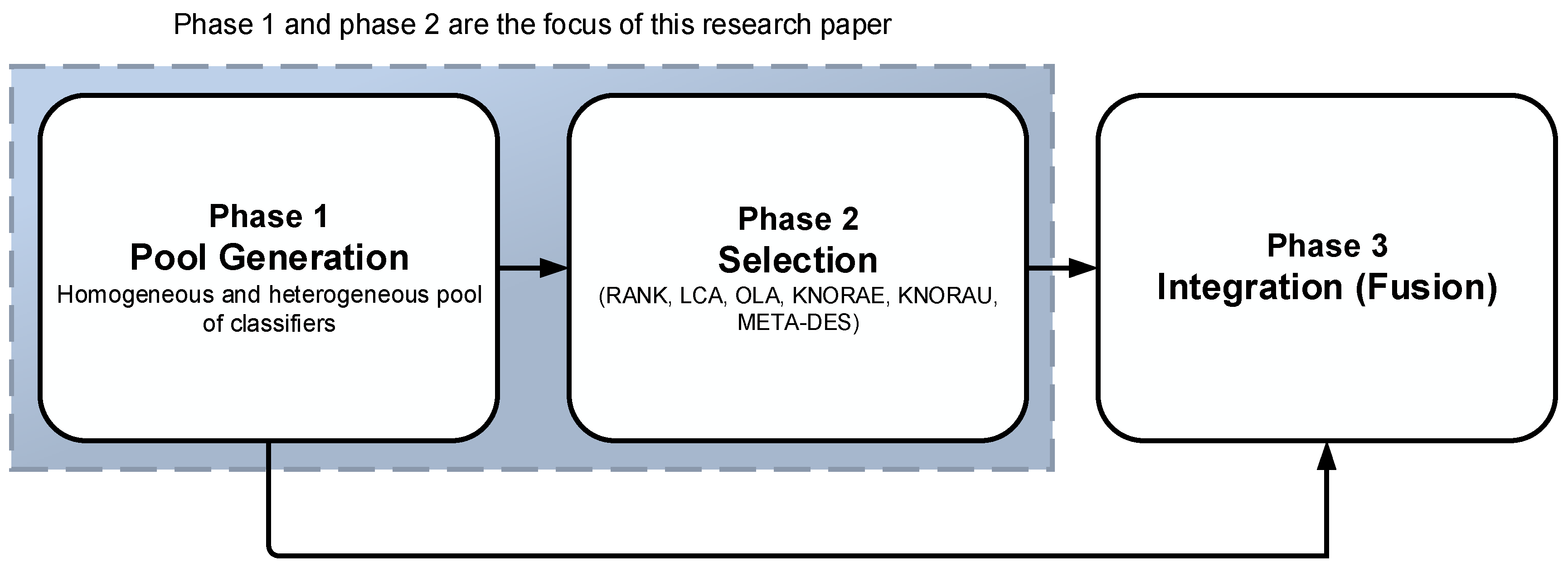
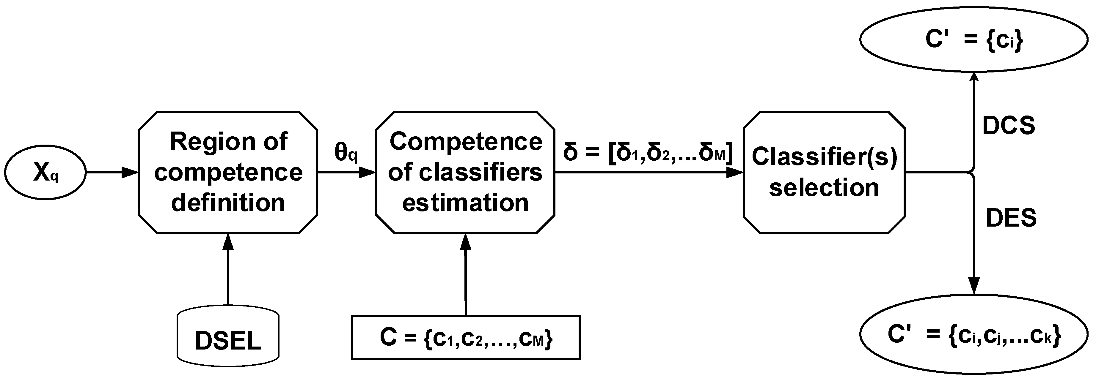
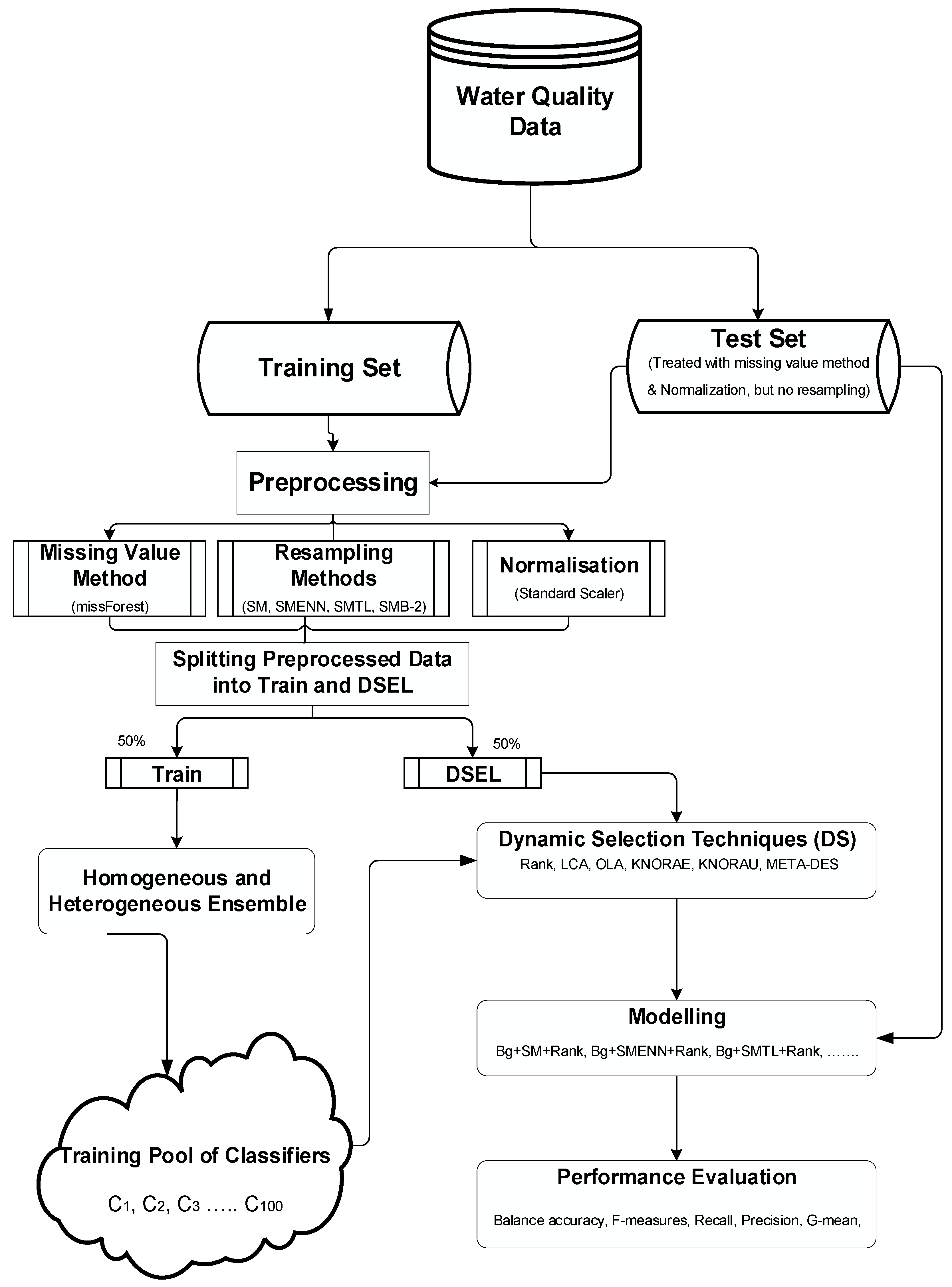
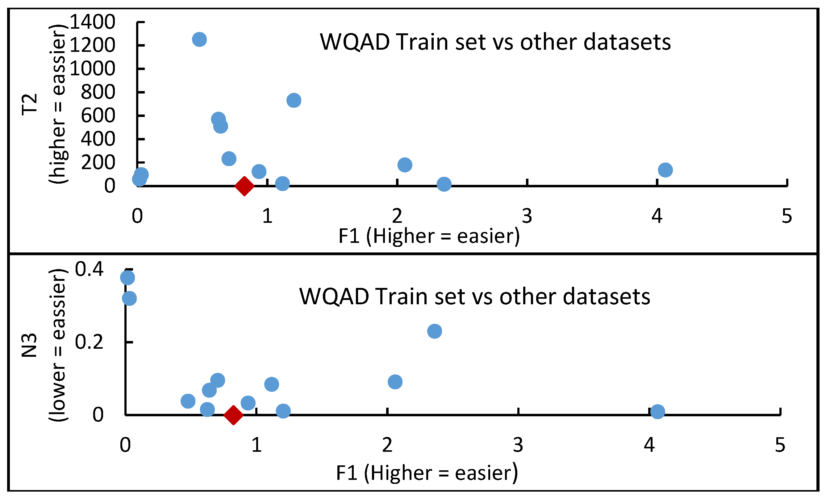
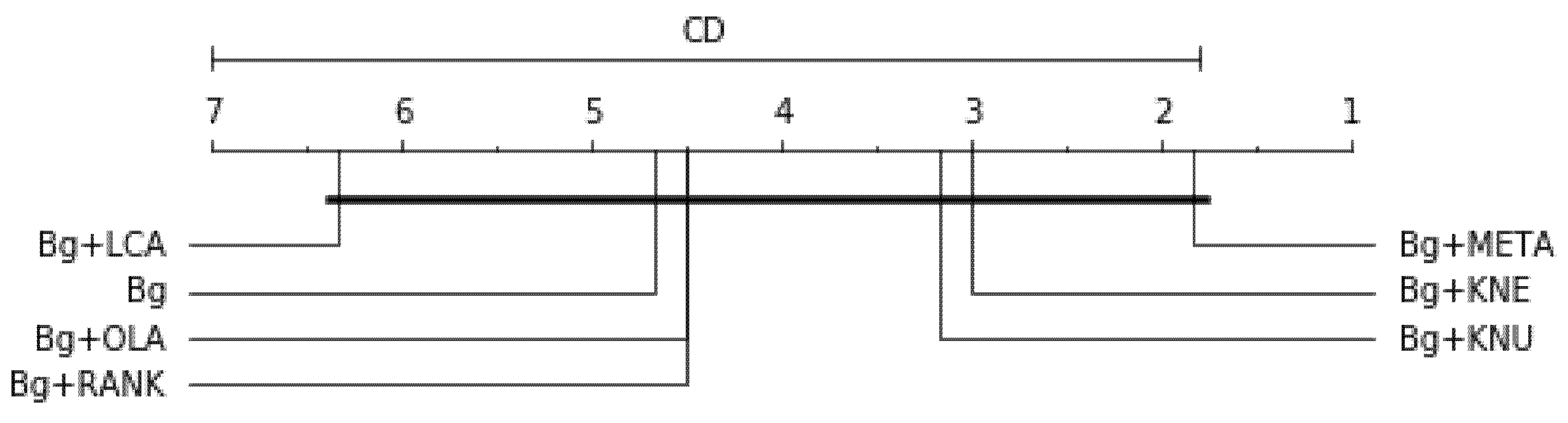
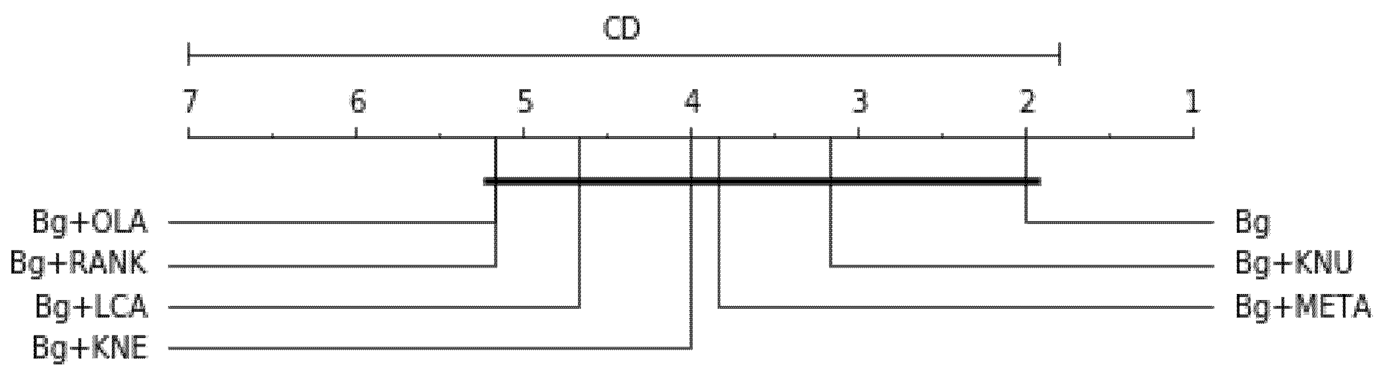
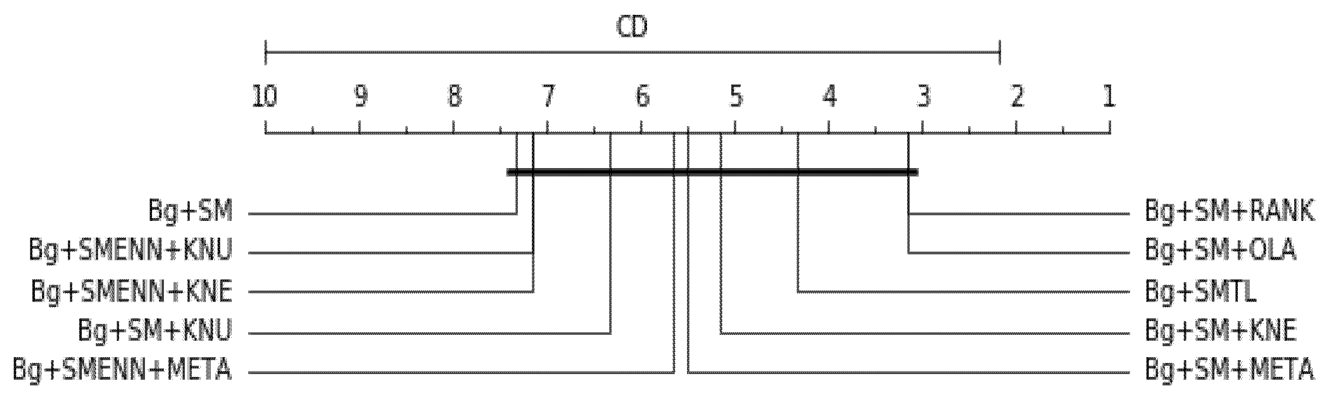
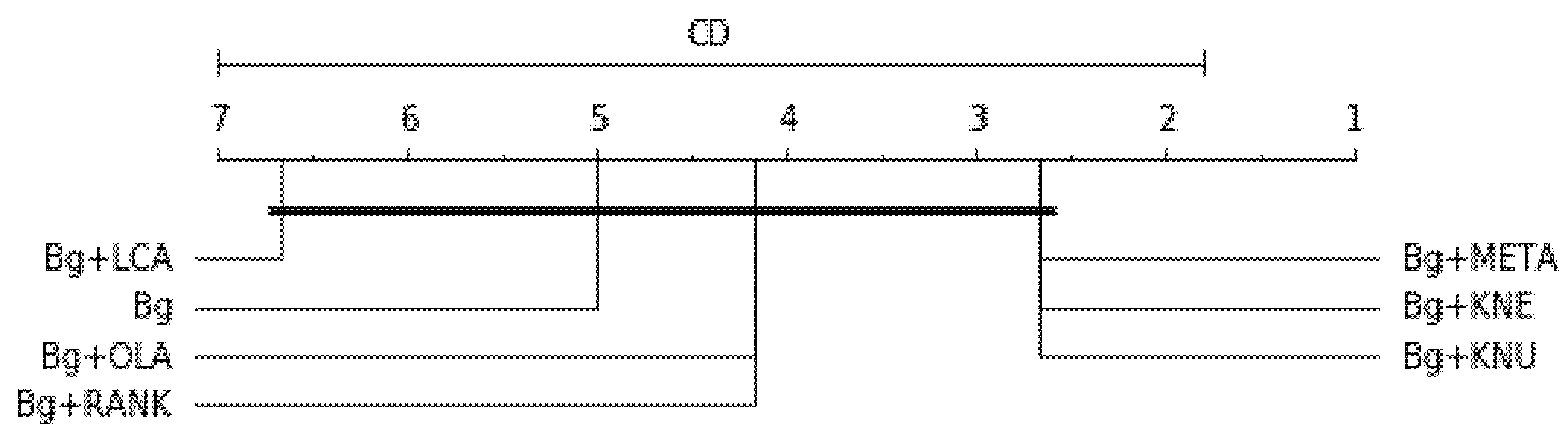
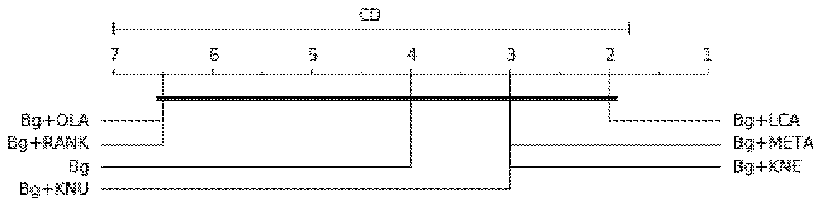
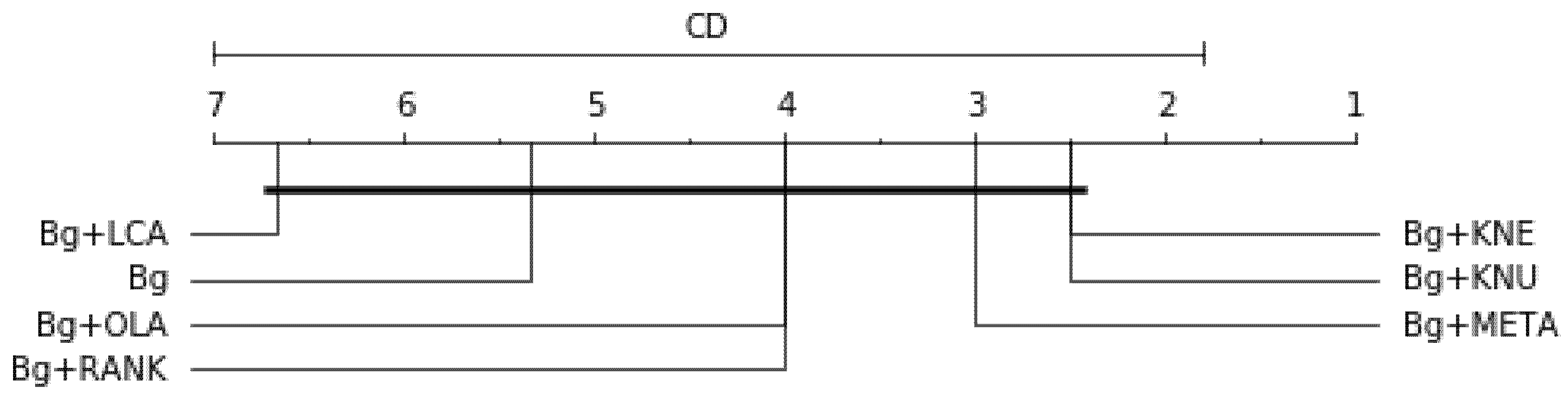
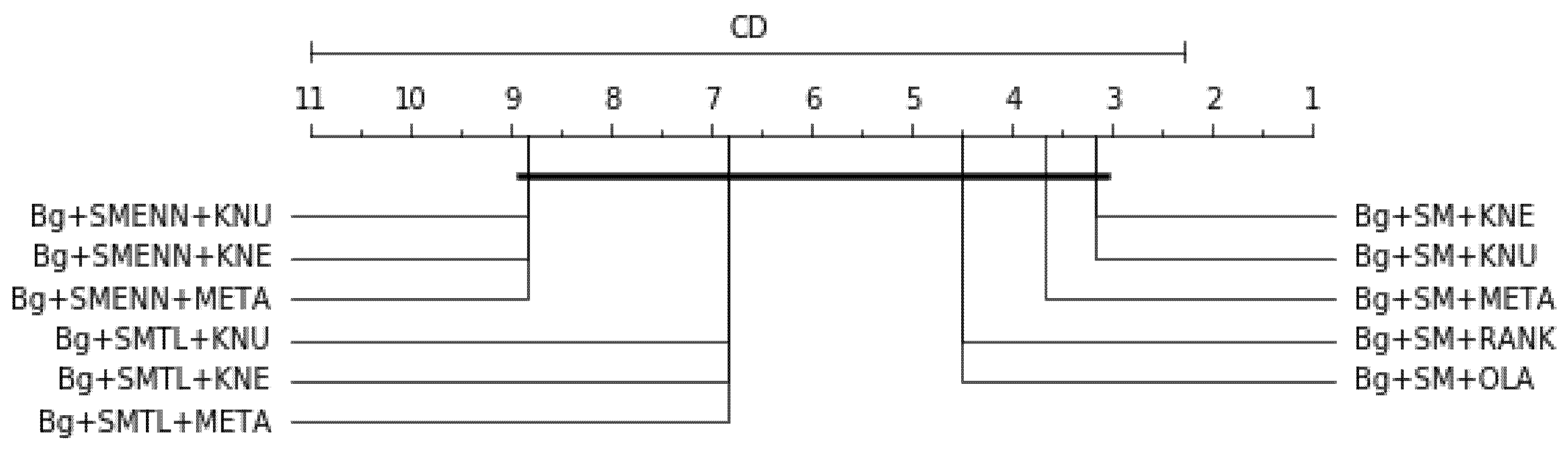
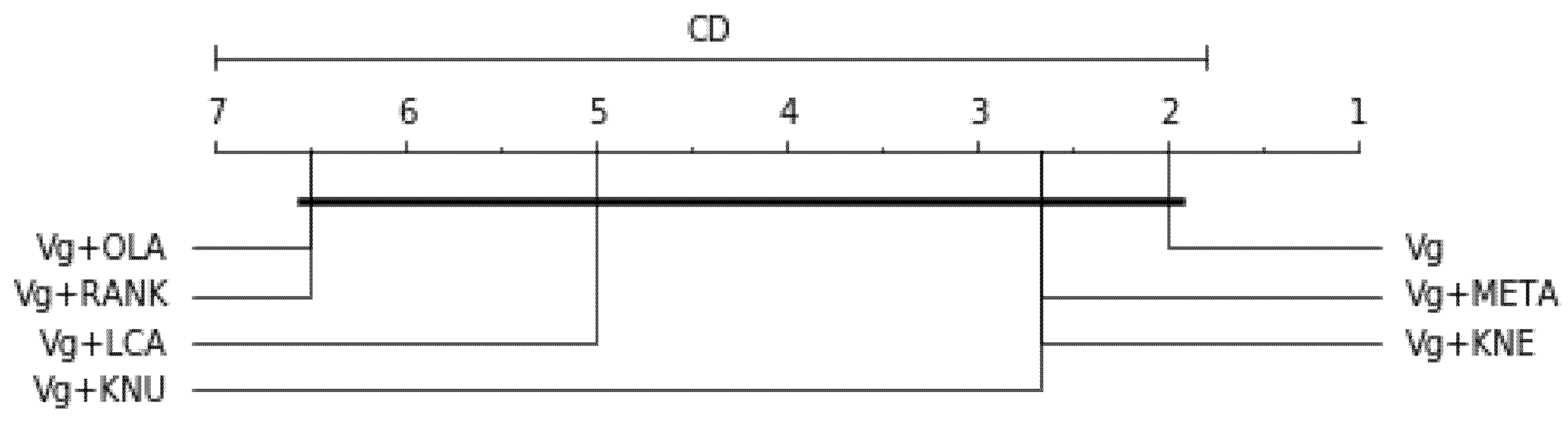
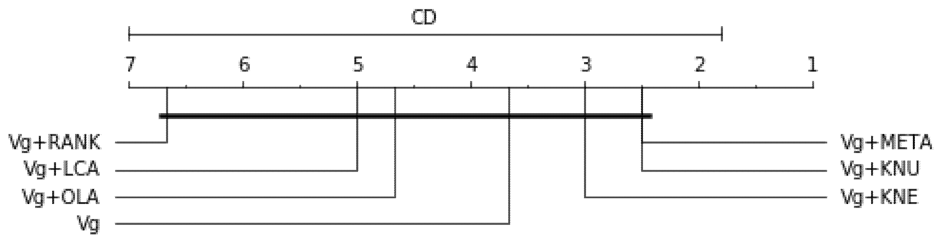
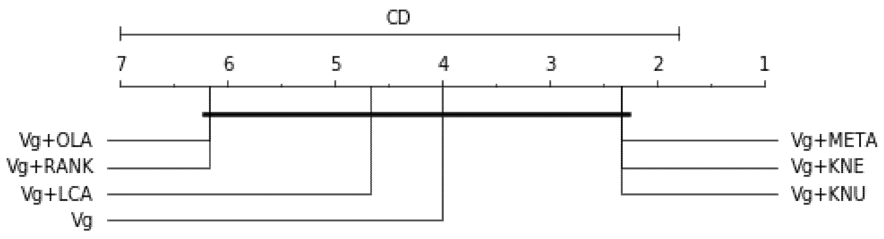
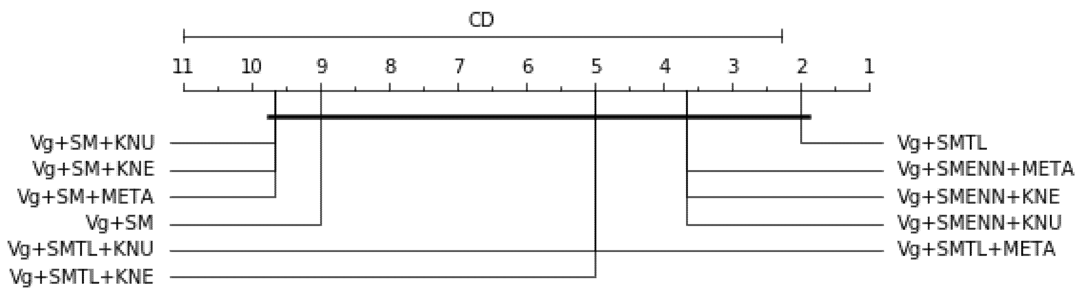
Table 1.
Summary of dynamic selection methods tested.
| # | DS Strategy | Competence Region Definition | Selection Criteria | Selection Strategy |
|---|---|---|---|---|
| 1. | Modified Class Rank (Rank) | K-NN | Ranking | DCS |
| 2. | Local Class Accuracy (LCA) | K-NN | Accuracy | DCS |
| 3 | Overall-Local Accuracy (OLA) | K-NN | Accuracy | DCS |
| 4. | K-Nearest Oracles Eliminate (KNORA-E) | K-NN | Oracle | DES |
| 5. | K-Nearest Oracles Union (KNORA-U) | K-NN | Oracle | DES |
| 6. | Meta-Learning for Dynamic Ensemble Selection (META-DES) | K-NN | Meta-learning | DES |
Table 2.
Summary of the models evaluated in the experiments.
| S/N | Ensemble Method | Description |
|---|---|---|
| Homogeneous (Base Classifier=dt and rf) and Heterogeneous (k-nn, rf, dt)–(voting classifier) | ||
| 1. | Bg+mF+SM | Bagging + missForest + SMOTE (Without DS method) |
| 2. | Bg+mF+SM+RANK | Bagging + missForest + SMOTE+ Modified Class Rank |
| 3. | Bg+mF+SM+LCA | Bagging + missForest + SMOTE + Local Classifier Accuracy |
| 4. | Bg+mF+SM+OLA | Bagging + missForest + SMOTE + Overall Local Accuracy |
| 5. | Bg+mF+SM+KNE | Bagging + missForest + SMOTE + K-Nearest Oracles Eliminate |
| 6. | Bg+mF+SM+KNU | Bagging + missForest + SMOTE + K-Nearest Oracles Union |
| 7. | Bg+mF+SM+META | Bagging + missForest + SMOTE + META-DES |
| 8. | Bg+mF+SMENN | Bagging + missForest + SMOTE-ENN (Without DS method) |
| 9. | Bg+mF+SMENN+RANK | Bagging + missForest + SMOTE-ENN + Modified Class Rank |
| 10. | Bg+mF+SMENN+LCA | Bagging + missForest + SMOTE-ENN + Local Classifier Accuracy |
| 11. | Bg+mF+SMENN+OLA | Bagging + missForest + SMOTE + ENN Overall Local Accuracy |
| 12. | Bg+mF+SMENN+KNE | Bagging + missForest + SMOTE-ENN + K-Nearest Oracles Eliminate |
| 13. | Bg+mF+SMENN+KNU | Bagging + missForest + SMOTE-ENN + K-Nearest Oracles Union |
| 14. | Bg+mF+SMENN+META | Bagging + missForest + SMOTE-ENN META-DES |
| 15. | Bg+mF+SMTL | Bagging + missForest + SMOTE-Tomek Links |
| 16. | Bg+mF+SMTL+RANK | Bagging + missForest + SMOTE-Tomek Links + Modified Rank |
| 17. | Bg+mF+SMTL+LCA | Bagging + missForest + SMOTE-Tomek Links + Local classifier accuracy |
| 18. | Bg+mF+SMTL+OLA | Bagging + missForest + SMOTE –Tomek Links + Overall Local Accuracy |
| 19. | Bg+mF+SMTL+KNE | Bagging + missForest + SMOTE-Tomek Links + K-Nearest Oracles Eliminate |
| 20. | Bg+mF+SMTL+KNU | Bagging + missForest + SMOTE-Tomek Links + K-Nearest Oracles Union |
| 21. | Bg+mF+SMTL+META | Bagging + missForest + SMOTE-Tomek Links + META-DES |
| 22. | Vg+mF+SM+RANK | VotingClassifier + missForest + SMOTE+ Modified Class Rank |
| 23. | Vg+mF+SM+LCA | VotingClassifier + missForest + SMOTE + Local Classifier Accuracy |
| 24. | Vg+mF+SM+OLA | VotingClassifier + missForest + SMOTE + Overall Local Accuracy |
| 25. | Vg+mF+SM+KNE | VotingClassifier + missForest + SMOTE + K-Nearest Oracles Eliminate |
| 26. | Vg+mF+SM+KNU | VotingClassifier + missForest + SMOTE + K-Nearest Oracles Union |
| 27. | Vg+mF+SM+META | VotingClassifier + missForest + SMOTE + META-DES |
| 28. | Vg+mF+SMENN+RANK | VotingClassifier + missForest + SMOTE-ENN + Modified Class Rank |
| 29. | Vg+mF+SMENN+LCA | VotingClassifier + missForest + SMOTE-ENN + Local Classifier Accuracy |
| 30. | Vg+mF+SMENN+OLA | VotingClassifier + missForest + SMOTE + ENN Overall Local Accuracy |
| 31. | Vg+mF+SMENN+KNE | VotingClassifier + missForest + SMOTE-ENN + K-Nearest Oracles Eliminate |
| 32. | Vg+mF+SMENN+KNU | VotingClassifier + missForest + SMOTE-ENN + K-Nearest Oracles Union |
| 33. | Vg+mF+SMENN+META | VotingClassifier + missForest + SMOTE-ENN META-DES |
| 34. | Vg+mF+SMTL+RANK | VotingClassifier + missForest + SMOTE-Tomek + Modified Rank |
| 35. | Vg+mF+SMTL+LCA | VotingClassifier + missForest + SMOTE-Tomek Link + Local classifier accuracy |
| 36. | Vg+mF+SMTL+OLA | VotingClassifier + missForest + SMOTE –Tomek Link + Overall Local Accuracy |
| 37. | Vg+mF+SMTL+KNE | VotingClassifier + missForest + SMOTE-Tomek Link + K-Nearest Oracles Eliminate |
| 38. | Vg+mF+SMTL+KNU | VotingClassifier + missForest + SMOTE-Tomek Link + K-Nearest Oracles Union |
| 39. | Vg+mF+SMTL+META | VotingClassifier + missForest + SMOTE-Tomek Link + META-DES |
Table 3.
Summary of dataset training and test sets characteristics.
| Dataset | Instances | Majority Class | Minority Class | Features | Class | Missing Values | Imbalance Ratio (Majority/Minority) |
|---|---|---|---|---|---|---|---|
| Training set | 139566 | 137840 | 1726 | 10 | 2 | 1044 | 79.86 |
| Test set | 139566 | 137237 | 2329 | 10 | 2 | 24480 | 58.93 |
Table 4.
Dataset features description.
| # | Features | Data Type | Unit | Description |
|---|---|---|---|---|
| 1. | Time | Categorical | dd/mm/yyyy HH:MM:SS | Date and Timestamp |
| 2. | Tp | Numerical | Degree Celsius (°C) | Water temperature |
| 3. | Cl_1 | Numerical | mg/L (MS1) | Amount of chlorine dioxide in the water of valve 1 |
| 4. | pH | Numerical | pH | pH value |
| 5. | Redox | Numerical | mV | Redox potential |
| 6. | Leit | Numerical | μS/cm | Electrical conductivity (EC) |
| 7. | Trueb | Numerical | NTU | Turbidity |
| 8. | Cl_2 | Numerical | mg/L (MS2) | Amount of chlorine dioxide in the water of valve 2 |
| 9. | Fm_1 | Numerical | m3/h | Flow Rate at valve 1 |
| 10. | Fm_2 | Numerical | m3/h | Flow Rate at valve 2 |
| 11. | EVENT | Boolean | Binary (Event) | Boolean anomaly label (0 or 1) |
Table 5.
Hyperparameter values tuning of methods evaluated using grid-search strategy.
| # | Method | Hyperparameter Values Tuned |
|---|---|---|
| 1. | k-nearest neighbor | n_neighbors = [3,5,10,15,20]; metric = [‘minkowski’, ‘manhattan’, weights = [‘uniform’, ‘distance’] |
| 2. | Support vector machine | kernel = [‘linear’ ‘poly’, ‘rbf’, ‘sigmoid’]; C = [1.0, 0.5, 0.1, 0.01]; gamma = [‘scale’] and class_weight = [‘balance’, ‘None’] |
| 3. | Random forest | n_estimators = [10,30,60,100] and max_features = [‘sqrt’, ‘log2’] |
| 4. | Easy Ensemble | |
| 5. | Decision tree | criterion = [‘gini’, ‘entropy’] and max_features = [‘sqrt’, ‘log2’] |
| 6. | AdaBoost | n_estimators = [10,30,60,100,200] and learning_rate = [0.1, 1.0] |
| 7. | RUSBoost | |
| 8. | Balanced Random Forest | n_estimators = [10,30,60,100], class_weight=[‘balanced’, ‘None’] and max_features = [] |
| 9. | Balanced Bagging Classifier | n_estimators = [10,30,60,100] and max_features = [] |
| 10. | HistGradientBoosting | learning_rate=[0.1, 1.0] and min_samples_leaf = [20,30,60] |
| 11. | Extra Trees | n_estimators = [10,30,60,100], max_features = [‘sqrt’, ‘log2’] and class_weight= [‘balanced’, ‘None’] |
| 12. | XGBoost | n_estimators = [10,30,60,100,200] and eta=learning_rate = [0.1, 0.3, 0.5, 1.0] |
| 13. | SMOTE | k_neighbors = [3,5,10,15,20]; sampling_strategy = [0.1, 0.3, 0.5, 1] |
| 14. | SMOTE+ENN | sampling_strategy = [0.1, 0.3, 0.5, 1] |
| 15. | SMOTE+Tomek Link | sampling_strategy = [0.1, 0.3, 0.5, 1] |
Table 6.
Confusion matrix for classification in a two-class problem.
| Predicted Positive (Class-1) | Predicted Negative (Class-0) | |
|---|---|---|
| Actual Positive (Class-1) | True Positive (TP) | False Negative (FN) |
| Actual Negative (Class-0) | False Positive (FP) | True Negative (TN) |
Table 7.
List of the acronym used in this paper.
| Acronym | Description | Acronym | Description |
|---|---|---|---|
| EASY | Easy Ensemble Classifier | DST | Decision Trees |
| RUSB | RUSBoost | SVM | Support Vector Machine |
| BRDF | Balanced Random Forest Classifier | STK 1 | Stacking Classifier 1 |
| BBAG | Balanced Bagging | STK 2 | Stacking Classifier 2 |
| HGDB | HistGradientBoosting | STK 3 | Stacking Classifier 3 |
| EXTR | Extra Trees | STK 4 | Stacking Classifier 4 |
| XGBT | XGBoost | DC | Default setting base classifier |
| k-NN | K-Nearest Neighbors | OC | Optimised base classifier |
| RDF | Random Forest | OR | Optimised resampling method |
| ADB | AdaBoost | DR | Default setting resampling method |
Table 8.
Complexity measures result in the training and test sets.
| Dataset | Complexity Measures | ||||||||
|---|---|---|---|---|---|---|---|---|---|
| F1 | F1v | F2 | F3 | F4 | N3 | T2 | T3 | T4 | |
| Training set | 0.824 | 3.322 × 10⁻⁸ | 4.79 × 10⁻⁴ | 0.979 | 0.886 | 4.33 × 10⁻⁴ | 6.497 × 10⁻⁵ | 5.775 × 10⁻⁵ | 0.889 |
| Test set | 0.857 | 5.964 × 10⁻⁸ | 1.187 × 10⁻⁵ | 0.993 | 0.978 | 2.17 × 10⁻³ | 7.820 × 10⁻⁵ | 6.951 × 10⁻⁵ | 0.889 |
Table 9.
Results with hyperparameter tuning of non-ensemble and static ensemble classifiers.
| Stk 4 | (k-nn, rf, dt, rbf kernel svm, adb) | Stk 3 | (k-nn, rf, dt, adb) | Stk 2 | (rf, k-nn, adb) | Stk 1 | (k-nn, adb) | SVM | DST | AdB | RDF | k-NN | XGBT | EXTr | HGDB | BBAG | BRDF | RUSB | EASY | MODEL | |
|---|---|---|---|---|---|---|---|---|---|---|---|---|---|---|---|---|---|---|---|---|---|
| 0.602 | 0.602 | 0.641 | 0.569 | 0.787 | 0.615 | 0.705 | 0.645 | 0.569 | 0.787 | 0.619 | 0.628 | 0.648 | 0.649 | 0.725 | 0.805 | B_acc | Metric | ||||
| 0.249 | 0.249 | 0.325 | 0.16 | 0.161 | 0.224 | 0.501 | 0.326 | 0.16 | 0.541 | 0.379 | 0.407 | 0.4 | 0.194 | 0.598 | 0.159 | F1 | |||||
| 0.212 | 0.212 | 0.289 | 0.151 | 0.691 | 0.246 | 0.413 | 0.299 | 0.151 | 0.584 | 0.237 | 0.256 | 0.3 | 0.335 | 0.451 | 0.738 | Recall | |||||
| 0.302 | 0.302 | 0.372 | 0.171 | 0.091 | 0.207 | 0.637 | 0.359 | 0.171 | 0.504 | 0.942 | 0.987 | 0.601 | 0.136 | 0.885 | 0.089 | Precision | |||||
| 0.459 | 0.459 | 0.536 | 0.386 | 0.781 | 0.492 | 0.641 | 0.544 | 0.386 | 0.76 | 0.487 | 0.506 | 0.547 | 0.568 | 0.671 | 0.802 | G-mean | |||||
Table 10.
Results for homogeneous bagging-based ensemble approach combined with DS methods using the optimised decision tree as a base estimator (pool of estimators = 100).
Table 10.
Results for homogeneous bagging-based ensemble approach combined with DS methods using the optimised decision tree as a base estimator (pool of estimators = 100).
| Resampling Method | Model | Performance Metric | ||||||
|---|---|---|---|---|---|---|---|---|
| B_acc | F1 | Recall | Precision | G-Mean | Training Time (s) | |||
| SMOTE | Bg+mF+SM | OC+DR | 0.629 | 0.307 | 0.266 | 0.365 | 0.514 | 24.772 |
| OC+OR | 0.633 | 0.314 | 0.274 | 0.369 | 0.521 | 15.040 | ||
| Bg+mF+SM+META | OC+DR | 0.686 | 0.133 | 0.465 | 0.078 | 0.650 | 2287.603 | |
| OC+OR | 0.734 | 0.212 | 0.527 | 0.133 | 0.704 | 663.323 | ||
| Bg+mF+SM+KNE | OC+DR | 0.684 | 0.133 | 0.462 | 0.078 | 0.647 | 28.574 | |
| OC+OR | 0.734 | 0.221 | 0.523 | 0.140 | 0.703 | 16.624 | ||
| Bg+mF+SM+KNU | OC+DR | 0.684 | 0.133 | 0.462 | 0.078 | 0.647 | 27.824 | |
| OC+OR | 0.733 | 0.220 | 0.520 | 0.140 | 0.701 | 16.992 | ||
| Bg+mF+SM+RANK | OC+DR | 0.642 | 0.072 | 0.486 | 0.039 | 0.623 | 28.252 | |
| OC+OR | 0.786 | 0.294 | 0.616 | 0.193 | 0.768 | 17.079 | ||
| Bg+mF+SM+LCA | OC+DR | 0.580 | 0.148 | 0.180 | 0.125 | 0.420 | 28.679 | |
| OC+OR | 0.618 | 0.277 | 0.245 | 0.320 | 0.495 | 16.575 | ||
| Bg+mF+SM+OLA | OC+DR | 0.642 | 0.072 | 0.486 | 0.039 | 0.623 | 28.373 | |
| OC+OR | 0.786 | 0.294 | 0.616 | 0.193 | 0.768 | 16.933 | ||
| SMOTE+ENN | Bg+mF+SMENN | OC+DR | 0.629 | 0.291 | 0.268 | 0.319 | 0.515 | 32.597 |
| OC+OR | 0.630 | 0.293 | 0.270 | 0.321 | 0.517 | 25.175 | ||
| Bg+mF+SMENN+META | OC+DR | 0.642 | 0.300 | 0.300 | 0.300 | 0.540 | 2506.205 | |
| OC+OR | 0.646 | 0.302 | 0.303 | 0.301 | 0.547 | 677.189 | ||
| Bg+mF+SMENN+KNE | OC+DR | 0.641 | 0.300 | 0.300 | 0.295 | 0.542 | 36.079 | |
| OC+OR | 0.645 | 0.300 | 0.301 | 0.299 | 0.545 | 27.321 | ||
| Bg+mF+SMENN+KNU | OC+DR | 0.643 | 0.298 | 0.300 | 0.299 | 0.542 | 35.634 | |
| OC+OR | 0.645 | 0.300 | 0.301 | 0.300 | 0.545 | 27.512 | ||
| Bg+mF+SMENN+RANK | OC+DR | 0.571 | 0.057 | 0.292 | 0.032 | 0.498 | 36.565 | |
| OC+OR | 0.571 | 0.057 | 0.292 | 0.032 | 0.498 | 27.659 | ||
| Bg+mF+SMENN+LCA | OC+DR | 0.566 | 0.115 | 0.159 | 0.091 | 0.393 | 37.094 | |
| OC+OR | 0.566 | 0.115 | 0.159 | 0.091 | 0.393 | 27.915 | ||
| Bg+mF+SMENN+OLA | OC+DR | 0.571 | 0.057 | 0.292 | 0.032 | 0.498 | 35.918 | |
| OC+OR | 0.571 | 0.057 | 0.292 | 0.032 | 0.498 | 28.222 | ||
| SMOTE+TL | Bg+mF+SMTL | OC+DR | 0.638 | 0.277 | 0.291 | 0.264 | 0.535 | 33.064 |
| OC+OR | 0.696 | 0.331 | 0.410 | 0.277 | 0.635 | 25.937 | ||
| Bg+mF+SMTL+META | OC+DR | 0.635 | 0.304 | 0.280 | 0.334 | 0.526 | 2535.888 | |
| OC+OR | 0.717 | 0.233 | 0.479 | 0.154 | 0.676 | 655.614 | ||
| Bg+mF+SMTL+KNE | OC+DR | 0.635 | 0.307 | 0.278 | 0.343 | 0.525 | 36.771 | |
| OC+OR | 0.715 | 0.252 | 0.468 | 0.172 | 0.671 | 28.317 | ||
| Bg+mF+SMTL+KNU | OC+DR | 0.634 | 0.306 | 0.278 | 0.342 | 0.525 | 36.486 | |
| OC+OR | 0.716 | 0.253 | 0.471 | 0.173 | 0.673 | 28.516 | ||
| Bg+mF+SMTL+RANK | OC+DR | 0.609 | 0.167 | 0.248 | 0.126 | 0.490 | 36.659 | |
| OC+OR | 0.561 | 0.046 | 0.369 | 0.025 | 0.527 | 28.356 | ||
| Bg+mF+SMTL+LCA | OC+DR | 0.573 | 0.156 | 0.161 | 0.150 | 0.399 | 37.098 | |
| OC+OR | 0.592 | 0.200 | 0.196 | 0.205 | 0.440 | 27.730 | ||
| Bg+mF+SMTL+OLA | OC+DR | 0.609 | 0.167 | 0.248 | 0.126 | 0.490 | 36.834 | |
| OC+OR | 0.561 | 0.046 | 0.369 | 0.025 | 0.527 | 27.877 | ||
Table 11.
Results for homogeneous bagging-based ensemble approach combined with DS methods using the optimised Random Forest as a base estimator (pool of estimators = 100).
Table 11.
Results for homogeneous bagging-based ensemble approach combined with DS methods using the optimised Random Forest as a base estimator (pool of estimators = 100).
| Resampling Method | Model | Performance Metric | ||||||
|---|---|---|---|---|---|---|---|---|
| B_acc | F1 | Recall | Precision | G-Mean | Training Time (s) | |||
| SMOTE | Bg+mF+SM | OC+DR | 0.636 | 0.313 | 0.281 | 0.354 | 0.528 | 137.030 |
| OC+OR | 0.643 | 0.321 | 0.295 | 0.351 | 0.541 | 83.127 | ||
| Bg+mF+SM+META | OC+DR | 0.636 | 0.281 | 0.284 | 0.279 | 0.530 | 424.557 | |
| OC+OR | 0.739 | 0.355 | 0.499 | 0.275 | 0.690 | 80.660 | ||
| Bg+mF+SM+KNE | OC+DR | 0.636 | 0.281 | 0.284 | 0.278 | 0.530 | 152.451 | |
| OC+OR | 0.739 | 0.355 | 0.499 | 0.275 | 0.699 | 90.355 | ||
| Bg+mF+SM+KNU | OC+DR | 0.636 | 0.281 | 0.284 | 0.279 | 0.530 | 150.710 | |
| OC+OR | 0.739 | 0.355 | 0.499 | 0.275 | 0.699 | 92.046 | ||
| Bg+mF+SM+RANK | OC+DR | 0.625 | 0.242 | 0.267 | 0.221 | 0.512 | 150.640 | |
| OC+OR | 0.742 | 0.259 | 0.528 | 0.171 | 0.711 | 91.948 | ||
| Bg+mF+SM+LCA | OC+DR | 0.617 | 0.307 | 0.240 | 0.425 | 0.489 | 151.089 | |
| OC_OR | 0.650 | 0.354 | 0.307 | 0.418 | 0.552 | 91.639 | ||
| Bg+mF+SM+OLA | OC+DR | 0.625 | 0.242 | 0.267 | 0.221 | 0.512 | 151.464 | |
| OC+OR | 0.742 | 0.259 | 0.528 | 0.171 | 0.711 | 91.352 | ||
| SMOTE+ENN | Bg+mF+SMENN | OC+DR | 0.636 | 0.311 | 0.280 | 0.306 | 0.527 | 143.380 |
| OC+OR | 0.702 | 0.354 | 0.421 | 0.350 | 0.643 | 93.799 | ||
| Bg+mF+SMENN+META | OC+DR | 0.639 | 0.326 | 0.286 | 0.381 | 0.532 | 429.103 | |
| OC+OR | 0.709 | 0.264 | 0.451 | 0.187 | 0.660 | 235.195 | ||
| Bg+mF+SMENN+KNE | OC+DR | 0.639 | 0.326 | 0.286 | 0.381 | 0.532 | 158.018 | |
| OC+OR | 0.709 | 0.264 | 0.451 | 0.187 | 0.660 | 102.839 | ||
| Bg+mF+SMENN+KNU | OC+DR | 0.639 | 0.326 | 0.286 | 0.381 | 0.532 | 158.615 | |
| OC+OR | 0.709 | 0.264 | 0.451 | 0.187 | 0.660 | 101.156 | ||
| Bg+mF+SMENN+RANK | OC+DR | 0.635 | 0.260 | 0.286 | 0.239 | 0.531 | 159.636 | |
| OC+OR | 0.694 | 0.248 | 0.421 | 0.175 | 0.638 | 101.914 | ||
| Bg+mF+SMENN+LCA | OC+DR | 0.625 | 0.351 | 0.254 | 0.567 | 0.503 | 157.479 | |
| OC+OR | 0.658 | 0.410 | 0.319 | 0.574 | 0.564 | 102.472 | ||
| Bg+mF+SMENN+OLA | OC+DR | 0.635 | 0.260 | 0.286 | 0.239 | 0.531 | 156.804 | |
| OC+OR | 0.694 | 0.248 | 0.421 | 0.175 | 0.638 | 102.266 | ||
| SMOTE+TL | Bg+mF+SMTL | OC+DR | 0.641 | 0.325 | 0.290 | 0.369 | 0.536 | 145.654 |
| OC+OR | 0.695 | 0.276 | 0.416 | 0.206 | 0.637 | 93.837 | ||
| Bg+mF+SMTL+META | OC+DR | 0.638 | 0.299 | 0.286 | 0.313 | 0.532 | 494.437 | |
| OC+OR | 0.712 | 0.334 | 0.445 | 0.267 | 0.660 | 267.526 | ||
| Bg+mF+SMTL+KNE | OC+DR | 0.638 | 0.299 | 0.286 | 0.313 | 0.532 | 159.036 | |
| OC+OR | 0.712 | 0.334 | 0.445 | 0.267 | 0.660 | 102.752 | ||
| Bg+mF+SMTL+KNU | OC+DR | 0.638 | 0.299 | 0.286 | 0.313 | 0.532 | 159.767 | |
| OC+OR | 0.712 | 0.334 | 0.445 | 0.267 | 0.660 | 102.799 | ||
| Bg+mF+SMTL+RANK | OC+DR | 0.652 | 0.330 | 0.315 | 0.347 | 0.558 | 158.567 | |
| OC+OR | 0.689 | 0.201 | 0.426 | 0.131 | 0.637 | 103.741 | ||
| Bg+mF+SMTL+LCA | OC+DR | 0.615 | 0.319 | 0.234 | 0.503 | 0.482 | 157.489 | |
| OC+OR | 0.636 | 0.364 | 0.277 | 0.531 | 0.525 | 104.609 | ||
| Bg+mF+SMTL+OLA | OC+DR | 0.652 | 0.330 | 0.315 | 0.347 | 0.558 | 158.993 | |
| OC+OR | 0.689 | 0.201 | 0.426 | 0.131 | 0.637 | 103.562 | ||
Table 12.
Results for heterogeneous ensemble (voting classifier) approach comprising three optimised k-NN, decision tree and random forest as the pool of classifiers in combination with DS methods.
Table 12.
Results for heterogeneous ensemble (voting classifier) approach comprising three optimised k-NN, decision tree and random forest as the pool of classifiers in combination with DS methods.
| Resampling Method | Model | Performance Metric | ||||||
|---|---|---|---|---|---|---|---|---|
| B_acc | F1 | Recall | Precision | G-Mean | Training Time (s) | |||
| SMOTE | Vg+mF+SM | OC+DR | 0.622 | 0.283 | 0.254 | 0.319 | 0.502 | 77.408 |
| OC+OR | 0.641 | 0.230 | 0.306 | 0.184 | 0.547 | 70.205 | ||
| Vg+mF+SM+META | OC+DR | 0.623 | 0.241 | 0.260 | 0.225 | 0.506 | 272.770 | |
| OC+OR | 0.634 | 0.236 | 0.288 | 0.200 | 0.531 | 99.401 | ||
| Vg+mF+SM+KNE | OC+DR | 0.623 | 0.241 | 0.260 | 0.225 | 0.506 | 37.473 | |
| OC+OR | 0.634 | 0.236 | 0.288 | 0.200 | 0.531 | 24.490 | ||
| Vg+mF+SM+KNU | OC+DR | 0.623 | 0.241 | 0.260 | 0.225 | 0.506 | 38.549 | |
| OC+OR | 0.634 | 0.236 | 0.288 | 0.200 | 0.531 | 24.801 | ||
| Vg+mF+SM+RANK | OC+DR | 0.568 | 0.151 | 0.149 | 0.153 | 0.384 | 37.975 | |
| OC+OR | 0.587 | 0.209 | 0.185 | 0.241 | 0.428 | 24.330 | ||
| Vg+mF+SM+LCA | OC+DR | 0.578 | 0.160 | 0.172 | 0.149 | 0.411 | 37.721 | |
| OC+OR | 0.594 | 0.226 | 0.198 | 0.263 | 0.442 | 24.542 | ||
| Vg+mF+SM+OLA | OC+DR | 0.568 | 0.151 | 0.149 | 0.153 | 0.384 | 38.072 | |
| OC+OR | 0.587 | 0.209 | 0.185 | 0.241 | 0.428 | 24.137 | ||
| SMOTE+ENN | Vg+mF+SMENN | OC+DR | 0.602 | 0.249 | 0.212 | 0.302 | 0.459 | 83.422 |
| OC+OR | 0.620 | 0.226 | 0.258 | 0.201 | 0.504 | 66.978 | ||
| Vg+mF+SMENN+META | OC+DR | 0.607 | 0.256 | 0.224 | 0.299 | 0.471 | 277.634 | |
| OC+OR | 0.699 | 0.280 | 0.426 | 0.208 | 0.644 | 148.286 | ||
| Vg+mF+SMENN+KNE | OC+DR | 0.607 | 0.256 | 0.224 | 0.299 | 0.471 | 47.621 | |
| OC+OR | 0.699 | 0.280 | 0.426 | 0.208 | 0.644 | 34.371 | ||
| Vg+mF+SMENN+KNU | OC+DR | 0.607 | 0.256 | 0.224 | 0.299 | 0.471 | 51.190 | |
| OC+OR | 0.699 | 0.280 | 0.426 | 0.208 | 0.644 | 34.654 | ||
| Vg+mF+SMENN+RANK | OC+DR | 0.568 | 0.152 | 0.150 | 0.153 | 0.385 | 49.381 | |
| OC+OR | 0.586 | 0.216 | 0.180 | 0.271 | 0.422 | 34.809 | ||
| Vg+mF+SMENN+LCA | OC+DR | 0.575 | 0.163 | 0.164 | 0.163 | 0.402 | 48.140 | |
| OC+OR | 0.605 | 0.261 | 0.217 | 0.327 | 0.464 | 34.387 | ||
| Vg+mF+SMENN+OLA | OC+DR | 0.568 | 0.152 | 0.150 | 0.153 | 0.385 | 48.981 | |
| OC+OR | 0.586 | 0.316 | 0.180 | 0.271 | 0.422 | 36.321 | ||
| SMOTE+TL | Vg+mF+SMTL | OC+DR | 0.615 | 0.261 | 0.240 | 0.284 | 0.488 | 76.781 |
| OC+OR | 0.700 | 0.375 | 0.413 | 0.343 | 0.639 | 82.793 | ||
| Vg+mF+SMTL+META | OC+DR | 0.614 | 0.243 | 0.240 | 0.247 | 0.487 | 277.722 | |
| OC+OR | 0.695 | 0.283 | 0.416 | 0.214 | 0.637 | 151.745 | ||
| Vg+mF+SMTL+KNE | OC+DR | 0.614 | 0.243 | 0.240 | 0.247 | 0.487 | 48.019 | |
| OC+OR | 0.695 | 0.283 | 0.416 | 0.214 | 0.637 | 34.916 | ||
| Vg+mF+SMTL+KNU | OC+DR | 0.614 | 0.243 | 0.240 | 0.247 | 0.487 | 47.457 | |
| OC+OR | 0.695 | 0.283 | 0.416 | 0.214 | 0.637 | 35.739 | ||
| Vg+mF+SMTL+RANK | OC+DR | 0.568 | 0.154 | 0.150 | 0.157 | 0.385 | 48.760 | |
| OC+OR | 0.587 | 0.210 | 0.183 | 0.245 | 0.426 | 34.777 | ||
| Vg+mF+SMTL+LCA | OC+DR | 0.575 | 0.164 | 0.165 | 0.163 | 0.404 | 47.630 | |
| OC+OR | 0.589 | 0.215 | 0.188 | 0.252 | 0.431 | 35.019 | ||
| Vg+mF+SMTL+OLA | OC+DR | 0.568 | 0.154 | 0.150 | 0.157 | 0.385 | 46.687 | |
| OC+OR | 0.587 | 0.210 | 0.183 | 0.245 | 0.426 | 34.821 | ||
Table 13.
Results for the average rank of the models based on each of the performance metric (Balanced accuracy, F1-measure and G-mean) considering the three resampling methods with decision tree as base the classifier.
Table 13.
Results for the average rank of the models based on each of the performance metric (Balanced accuracy, F1-measure and G-mean) considering the three resampling methods with decision tree as base the classifier.
| Balanced Accuracy | F1-Measure | G-Mean | |||
|---|---|---|---|---|---|
| Ensemble | Rank | Ensemble | Rank | Ensemble | Rank |
| Bg | 4.667 | Bg | 2.0 | Bg | 4.667 |
| Bg+META | 1.833 | Bg+META | 3.833 | Bg+META | 1.667 |
| Bg+KNE | 3.0 | Bg+KNE | 4.0 | Bg+KNE | 3.167 |
| Bg+KNU | 3.167 | Bg+KNU | 3.167 | Bg+KNU | 3.167 |
| Bg+RANK | 4.5 | Bg+RANK | 5.167 | Bg+RANK | 4.167 |
| Bg+LCA | 6.333 | Bg+LCA | 4.667 | Bg+LCA | 7.0 |
| Bg+OLA | 4.5 | Bg+OLA | 5.167 | Bg+OLA | 4.167 |
Table 14.
Overall results of the average rank of the 10 best models considering all the three performance metrics (Balanced accuracy, F1-measure and G-mean scores) across the three resampling methods with decision tree as the base classifier.
Table 14.
Overall results of the average rank of the 10 best models considering all the three performance metrics (Balanced accuracy, F1-measure and G-mean scores) across the three resampling methods with decision tree as the base classifier.
| Ensemble. | Rank | Ensemble | Rank |
|---|---|---|---|
| Bg+SM | 7.333 | Bg+SMTL+OLA | 3.167 |
| Bg+SM+META | 5.5 | Bg+SMENN+META | 5.667 |
| Bg+SM+KNE | 5.167 | Bg+SMENN+KNE | 7.167 |
| Bg+SM+KNU | 6.333 | Bg+SMENN+KNU | 7.167 |
| Bg+SM+RANK | 3.167 | Bg+SMTL | 4.333 |
Table 15.
Results of the average rank of the models based on each of the performance scores (Balanced accuracy, F1-measure and G-mean) considering the three resampling methods with the random forest as the base classifier.
Table 15.
Results of the average rank of the models based on each of the performance scores (Balanced accuracy, F1-measure and G-mean) considering the three resampling methods with the random forest as the base classifier.
| Balanced Accuracy | F1-Measure | G-Mean | |||
|---|---|---|---|---|---|
| Ensemble | Rank | Ensemble | Rank | Ensemble | Rank |
| Bg | 5.5 | Bg | 4.0 | Bg | 5.333 |
| Bg+META | 2.667 | Bg+META | 3.0 | Bg+META | 3.0 |
| Bg+KNE | 2.667 | Bg+KNE | 3.0 | Bg+KNE | 2.5 |
| Bg+KNU | 2.667 | Bg+KNU | 3.0 | Bg+KNU | 2.5 |
| Bg+RANK | 1.167 | Bg+RANK | 6.5 | Bg+RANK | 4.0 |
| Bg+LCA | 6.667 | Bg+LCA | 2.0 | Bg+LCA | 6.667 |
| Bg+OLA | 4.167 | Bg+OLA | 6.5 | Bg+OLA | 4.0 |
Table 16.
Overall results of the average rank of 10 best methods considering all the three performance scores (Balanced accuracy, F1 and G-mean scores) across the three resampling methods with the random forest as the base classifier.
Table 16.
Overall results of the average rank of 10 best methods considering all the three performance scores (Balanced accuracy, F1 and G-mean scores) across the three resampling methods with the random forest as the base classifier.
| Model | Rank |
|---|---|
| Bg+SM+META | 3.667 |
| Bg+SM+KNE | 3.167 |
| Bg+SM+KNU | 3.167 |
| Bg+SM+RANK | 4.5 |
| Bg+SM+OLA | 4.5 |
| Bg+SMENN+META | 8.833 |
| Bg+SMENN+KNE | 8.833 |
| Bg+SMENN+KNU | 8.833 |
| Bg+SMTL+META | 6.833 |
| Bg+SMTL+KNE | 6.833 |
| Bg+SMTL+KNU | 6.833 |
Table 17.
The average rank for best DS method based on balanced accuracy, F1-measure and G-mean with heterogeneous base classifiers.
Table 17.
The average rank for best DS method based on balanced accuracy, F1-measure and G-mean with heterogeneous base classifiers.
| Balanced Accuracy | F1-Measure | G-Mean | |||
|---|---|---|---|---|---|
| Model | Rank | Model | Rank | Model | Rank |
| Vg | 2.0 | Vg | 3.667 | Vg | 4.0 |
| Vg+META | 2.667 | Vg+META | 2.5 | Vg+META | 2.333 |
| Vg+KNE | 2.667 | Vg+KNE | 3.0 | Vg+KNE | 2.333 |
| Vg+KNU | 2.667 | Vg+KNU | 2.5 | Vg+KNU | 2.333 |
| Vg+RANK | 6.5 | Vg+RANK | 6.667 | Vg+RANK | 6.167 |
| Vg+LCA | 5.0 | Vg+LCA | 5.0 | Vg+LCA | 4.667 |
| Vg+OLA | 6.5 | Vg+OLA | 4.667 | Vg+OLA | 6.167 |
Table 18.
The average rank of 10 best methods considering all the three performance scores (Balanced accuracy, F1 and G-mean scores) across the three resampling methods.
Table 18.
The average rank of 10 best methods considering all the three performance scores (Balanced accuracy, F1 and G-mean scores) across the three resampling methods.
| Ensemble | Rank |
|---|---|
| Vg+SM | 9.0 |
| Vg+SM+META | 9.667 |
| Vg+SM+KNE | 9.667 |
| Vg+SM+KNU | 9.667 |
| Vg+SMENN+META | 3.667 |
| Vg+SMENN+KNE | 3.667 |
| Vg+SMENN+KNU | 3.667 |
| Vg+SMTL | 2.0 |
| Vg+SMTL+META | 5.0 |
| Vg+SMTL+KNE | 5.0 |
| Vg+SMTL+KNU | 5.0 |
Publisher’s Note: MDPI stays neutral with regard to jurisdictional claims in published maps and institutional affiliations. |
© 2021 by the authors. Licensee MDPI, Basel, Switzerland. This article is an open access article distributed under the terms and conditions of the Creative Commons Attribution (CC BY) license (https://creativecommons.org/licenses/by/4.0/).
Share and Cite
MDPI and ACS Style
Dogo, E.M.; Nwulu, N.I.; Twala, B.; Aigbavboa, C. Accessing Imbalance Learning Using Dynamic Selection Approach in Water Quality Anomaly Detection. Symmetry 2021, 13, 818. https://doi.org/10.3390/sym13050818
AMA Style
Dogo EM, Nwulu NI, Twala B, Aigbavboa C. Accessing Imbalance Learning Using Dynamic Selection Approach in Water Quality Anomaly Detection. Symmetry. 2021; 13(5):818. https://doi.org/10.3390/sym13050818
Chicago/Turabian StyleDogo, Eustace M., Nnamdi I. Nwulu, Bhekisipho Twala, and Clinton Aigbavboa. 2021. "Accessing Imbalance Learning Using Dynamic Selection Approach in Water Quality Anomaly Detection" Symmetry 13, no. 5: 818. https://doi.org/10.3390/sym13050818
Note that from the first issue of 2016, this journal uses article numbers instead of page numbers. See further details here.