
Validation of NOAA CyGNSS Wind Speed Product with the CCMP Data
by
 , , , and
Xiaohui Li
1,2 ,
,
Dongkai Yang
1,
Jingsong Yang
2,3,*,
Guoqi Han
4,
Gang Zheng
2,3 and
Weiqiang Li
5,6 1
School of Electronic and Information Engineering, Beihang University, Beijing 100191, China
2
State Key Laboratory of Satellite Ocean Environment Dynamics, Second Institute of Oceanography, Ministry of Natural Resources, Hangzhou 310012, China
3
Southern Marine Science and Engineering Guangdong Laboratory (Zhuhai), Zhuhai 519082, China
4
Fisheries and Oceans Canada, Institute of Ocean Sciences, Sidney, BC V8L 4B2, Canada
5
Institute of Space Sciences (ICE, CSIC), 08193 Barcelona, Spain
6
Institut d’Estudis Espacials de Catalunya (IEEC), 08034 Barcelona, Spain
*
Author to whom correspondence should be addressed.
Remote Sens. 2021, 13(9), 1832; https://doi.org/10.3390/rs13091832
Submission received: 28 February 2021
/
Revised: 21 April 2021
/
Accepted: 28 April 2021
/
Published: 7 May 2021
(This article belongs to the Special Issue Recent Advances in GNSS Reflectometry)
Abstract
:The National Aeronautics and Space Administration (NASA) Cyclone Global Navigation Satellite System (CyGNSS) mission was launched in December 2016, which can remotely sense sea surface wind with a relatively high spatio-temporal resolution for tracking tropical cyclones. In recent years, with the gradual development of the geophysical model function (GMF) for CyGNSS wind retrieval, different versions of CyGNSS Level 2 products have been released and their performance has gradually improved. This paper presents a comprehensive evaluation of CyGNSS wind product v1.1 produced by the National Oceanic and Atmospheric Administration (NOAA). The Cross-Calibrated Multi-Platform (CCMP) analysis wind (v02.0 and v02.1 near real time) products produced by Remote Sensing Systems (RSS) were used as the reference. Data pairs between the NOAA CyGNSS and RSS CCMP products were processed and evaluated by the bias and standard deviation SD. The CyGNSS dataset covers the period between May 2017 and December 2020. The statistical comparisons show that the bias and SD of CyGNSS relative to CCMP-nonzero collocations when the flag of CCMP winds is nonzero are –0.05 m/s and 1.19 m/s, respectively. The probability density function (PDF) of the CyGNSS winds coincides with that of CCMP-nonzero. Furthermore, the average monthly bias and SD show that CyGNSS wind is consistent and reliable generally. We found that negative deviation mainly appears at high latitudes in both hemispheres. Positive deviation appears in the China Sea, the Arabian Sea, and the west of Africa and South America. Spatial–temporal analysis demonstrates the geographical anomalies in the bias and SD of the CyGNSS winds, confirming that the wind speed bias shows a temporal dependency. The verification and comparison show that the remotely sensed wind speed measurements from NOAA CyGNSS wind product v1.1 are in good agreement with CCMP winds.
1. Introduction
Sea surface wind is an important physical parameter in oceanography, as it regulates the spatial distribution of air–sea fluxes of heat, moisture, gases, momentum, and other physical parameters, thus determining and maintaining the air–sea interactions and atmospheric dynamics [1,2,3,4]. In the process of ocean dynamics, sea surface wind is the most influential factor in the generation of ocean hydroynamic phenomena such as wind waves. It not only plays a role in global and regional ocean circulation, but also in weather forecasting and other atmospheric and oceanographic science studies [5,6,7,8]. Consequently, the adequate and accurate description of sea surface wind fields is important for related research [9].
In terms of accuracy, the conventional in situ measurements from meteorological stations, buoys, and ships are the most reliable among the available ocean wind data [1]. These types of data also have some limitations. The effective observation range of these measurements is limited due to technical means. Although the accuracy of buoy data is high, it is limited by the number of buoys. Buoys are mainly distributed in the coastal areas of the northern hemisphere. Measurements from ships may be contaminated by ship motion; many survey reports are geographically biased [1]. Satellite remote sensing is capable of systematically providing large-area synchronous measurements over the entire globe [4,10,11,12,13], which complement existing techniques. High-spatial-resolution sea surface wind fields can be provided by synthetic aperture radar (SAR). SAR has obvious advantages in monitoring inshore wind and numerical applications [14,15,16,17,18,19,20,21]. Due to the high cost of imaging, it is impossible to continuously observe a specific area. Scatterometry and radiometry have been efficiently used for monitoring sea surface winds from space during the last several decades [22,23]. However, they are insufficient for current science studies due to the satellite’s long revisit cycle and irregular spatial coverage. Currently, gridded wind data can be effectively simulated by numerical models. Moreover, numerical models can assimilate satellite remote sensing data to generate reanalysis data. Several kinds of gridded wind field sources have been adopted, e.g., European Centre for Medium-Range Weather Forecasts (ECMWF) reanalysis data [24], National Centers for Environmental Prediction’s Climate Forecast System Reanalysis (NCEP-CFSR) data [25], and the Cross-Calibrated Multi-Platform (CCMP) analysis data produced by Remote Sensing Systems (RSS) [26]. However, the reanalysis products always underestimate high wind speeds, especially in tropical cyclones [27,28].
The emergence of Global Satellite Navigation System (GNSS) has provided a new possibility for sensing sea surface wind speed. The concept of GNSS reflectometry (GNSS-R) was introduced for altimetry in 1993 [29]. Compared with active microwave instruments (scatterometers and altimeters), it is possible to observe ocean winds at a lower cost by using the freely available sea-surface-reflected GNSS signals. Theoretical work over the last decades has shown that the reflected GNSS signals can be used to retrieve the geophysical parameters such as ocean wind speed [30,31], significant wave height [32,33], sea ice [34,35], sea level [36,37,38], and surface soil moisture [39,40]. GNSS-R technology has been verified by a number of ground-based, airborne experiments [41,42,43,44,45,46,47,48]. Since the GPS reflection signal was detected from spaceborne sensors, the spaceborne GNSS-R missions were proposed [49]. The UK-Disaster Monitoring Constellation (UK-DMC) mission demonstrated the feasibility and validity of GNSS-R technology in 2004 [50]. Since then, the follow-on UK TechDemoSat-1 (TDS-1) was launched after UK-DMC successfully verified that the reflected GNSS signals can be used to retrieve geophysical parameters [51]. Furthermore, it was shown that GNSS-R has the ability to retrieve wind speed under rainfall conditions [52]. The retrieval performance of TDS-1 has been estimated during the TDS-1 mission period in previous studies [52,53,54,55]. Spatial and temporal variabilities of TDS-1 were also discussed, showing that it has large variability during the TDS-1 mission [55].
The CyGNSS mission was launched on 15 December 2016 by the National Aeronautics and Space Administration (NASA). This mission consists of eight micro-satellites, which enhance the spatial and temporal resolution of ocean wind data for monitoring tropical cyclones, typhoons, and hurricanes. This mission is intended to observe and understand tropical cyclones genesis and intensification, so as to improve prediction ability [56]. It has become one of the key constellations demonstrating the benefit of GNSS-R for monitoring ocean winds. BuFeng-1 A/B, as the first Chinese GNSS-R mission, was launched on 5 June 2019 [57]. The mission is constantly acquiring global sea surface wind data. In recent years, with the continuous improvements in the CyGNSS retrieval algorithm, its official wind speed products have been released. Evaluating the performance of sea surface wind products from CyGNSS has become an urgent issue for various applications. With the enhancement in the spaceborne GNSS-R sea wind retrieval algorithms, the performance of CyGNSS product has been improved [30,31,58,59,60]. Ref. [61] stated that the accuracy of the NASA CyGNSS Level 2 baseline surface ocean winds product by buoys is less than 2 m/s over the tropical and subtropical oceans [61]. Some evaluations of CyGNSS v1.0 wind produced by the NOAA have been compared against HWRF and ECMWF model winds, and remote sensing sea surface wind of scatterometers and radiometers, which demonstrated that the NOAA CyGNSS wind product has achieved its goals of consistency, reliability, and repeatability [62].
The validation of the NOAA CyGNSS wind product is important for its further applications in different areas. This paper reports a probe into the performance of the NOAA CyGNSS wind product against the CCMP one. A quantitative temporal and spatial comparison was implemented for the period between May 2017 and December 2020. The structure of this paper is as follows: The next Section provides a detailed description of the dataset and the processing method. In Section 2, the statistical comparison and validation results between the CyGNSS and CCMP wind on global scale are presented. A preliminary discussion is presented in Section 4. Section 5 draws the conclusions.
2. Data Set Description and Data Processing
In this study, the data sets of the RSS CCMP analysis wind product and NOAA CyGNSS v1.1 wind products were used. Brief descriptions of the data and method are provided below.
2.1. RSS CCMP Wind Product
The CCMP wind product was used to evaluate the performance of NOAA CyGNSS wind product. As an analysis product, the ECMWF ERA-Interim reanalysis winds are taken as the first-guess wind field. CCMP simultaneously integrates multisatellite sea surface winds of scatterometers from QuikSCAT and METOP-A/ASCAT; radiometers from SSM/I, SSMIS, AMSR, TMI, WindSat, and GMI; and in situ observations from NDBC, TAO, TRITON, RAMA, PIRATA, and Canadian [26,63]; and has its own unique characteristics. The spatial and temporal resolutions of CCMP are 0.25 and 6 h (00:00, 06:00, 12:00, and 18:00 UTC), respectively. Considering the continuity of wind field in space, multiple wind speed observations are usually sufficient to determine an accurate wind vector [64]. For each cell of CCMP, if there is no measured data (the nobs flag is zero), the background wind field is adopted. Such data from CCMP are named CCMP-zero. Otherwise, they are named CCMP-nonzero in this paper (Equation (1)). CCMP wind analyses data including U- and V-components were downloaded from Remote Sensing Systems (Available online: www.remss.com (accessed on 31 January 2021)), covering the period 2017–2020. Note that the CCMP v02.0 product during 2017–2018 and the near real-time Version-02.1 (v02.1.NRT) product during 2019–2020 were acquired for this study. Previous studies showed that the CCMP wind speed is closer to conventional in situ measurements from ships than ECMWF and NCEP-CFSR products [65]. CCMP winds and Tropical Atmosphere Ocean (TAO) mooring observations were compared, which showed good agreement with an root mean square error (RMSE) of 1 m/s and a correlation coefficient of 0.95 [66]. The CCMP wind product is a newly released global ocean wind dataset and suitable for scientific study at various temporal and spatial resolutions. We used the CCMP sea surface wind speeds to assess the performance of the NOAA CyGNSS product on the global scale.
2.2. NOAA CyGNSS Wind Product
The Cyclone GNSS (CyGNSS) mission was designed to observe ocean winds by a constellation of eight microsatellites with high spatial and temporal resolutions for quickly tracking tropical cyclones [56,67]. In this study, the quality of CyGNSS sea surface wind speed operational product reproduced by NOAA was assessed. The NOAA’s dataset is available at (https://manati.star.nesdis.noaa.gov/, (accessed on 31 January 2021)). The NOAA CyGNSS wind v1.1 product was used for comparison with the CCMP gridded surface wind analysis data product. Early studies of CyGNSS v1.0 and v1.1 retrievals and validation against ECMWF and ASCAT scatterometry observations were accomplished [62,68]. The standard deviation (SD) of overall CyGNSS v1.1 decreased from 1.33 to 1.19 m/s against ECMWF. Table 1 lists the wind speed requirements for the CyGNSS mission. The designed accuracy of CyGNSS mission is <2 m/s or <10% in RMSE for wind retrievals. Prior to launch, the mission design of the satellites and science payloads referred to these requirements. Once in orbit, they can be used to evaluate whether the mission is successful [69].
2.3. Along Track Retrieval Algorithm for NOAA CyGNSS
Considering the sensitivity of CyGNSS observation to the information of waves that are not generated by local winds, NOAA’s scientific team improved the performance of CyGNSS wind speed retrieval using a priori knowledge of the wave height as the input parameter [70,71]. In addition, NOAA’s Along Track Retrieval Algorithm (ATRA) is based on wind speed (), angle of incidence (), the significant wave height (), and CyGNSS , as shown in Equation (2). ATRA also uses track-wise processing to reduce the systematic errors due to the uncertainties of the transmitted power and receiver instrumental effects. A wind–wave GMF is presented for retrieving the sea surface wind speed along the track of CyGNSS. A detailed description of this algorithm is provided in [70].
2.4. Spatial and Temporal Collocation
Both CyGNSS and CCMP winds are provided at the height of 10 m above the sea surface in neutral conditions. Before matching, quality control was applied to remove poor-quality samples of NOAA CyGNSS according to quality flags (Equation (3) [72]). If = 0, then the wind speed samples were considered of good quality.
where is the variable in the NOAA Level 2 CyGNSS NetCDF file, is the function that returns the modulus after the division of by 2, and is the final quality of the flags used in this paper.
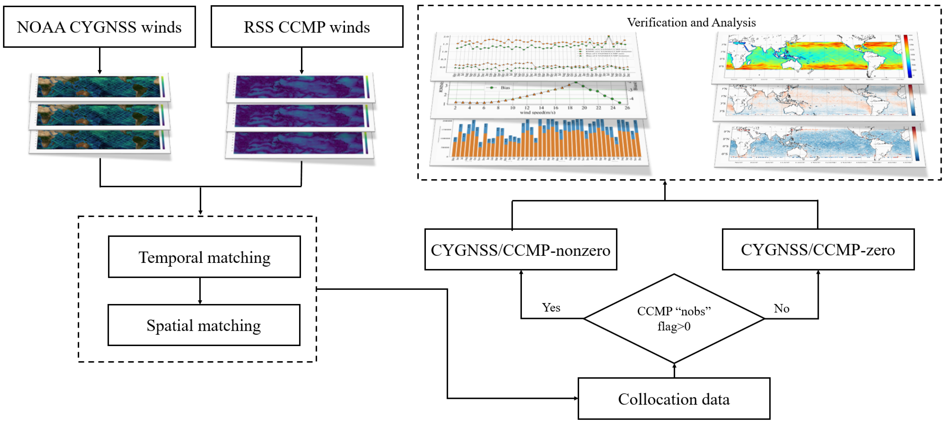
As sea surface states differ over time [5], it is necessary to ensure that the acquisition time of the CyGNSS measurement is close to that of CCMP wind speed. The spatial and temporal windows are the collocation criteria for ensuring the consistency of ocean winds observed by different sources. The CCMP winds were collocated with CyGNSS specular point using the closest cell in space and time. The following describes the detailed procedure of collocating CyGNSS and CCMP. First, considering the consistency of wind in time, the CyGNSS specular points were selected by a temporal window within ±5 min relative to the time of CCMP. Then, the nearest grid was located according to the center of a CyGNSS specular point’s longitude and latitude. Finally, the CyGNSS/CCMP collocations were obtained from the CCMP product. To compare and analyze the CyGNSS wind product, we extracted the sea surface wind speed that had the flag with nonzero observation numbers (nobs > 0) from CCMP. To compare the spatial distribution, CyGNSS winds were divided on a regular geographical grid of 1 by 1, and the metrics (bias and SD) were calculated against by the CCMP wind speed in every grid cell (Figure 1).
In this study, the deviation (Bias) and SD were the metrics used to quantitatively describe and evaluate the CyGNSS/CCMP collocations. Their definitions are as follows:
where x is NOAA CyGNSS v1.1 wind speed, y is CCMP wind speed, z is the difference between CyGNSS and CCMP, is the mean z, and n is the number of CyGNSS/CCMP collocations.
3. Results
3.1. Comparisons between CyGNSS and CCMP Winds
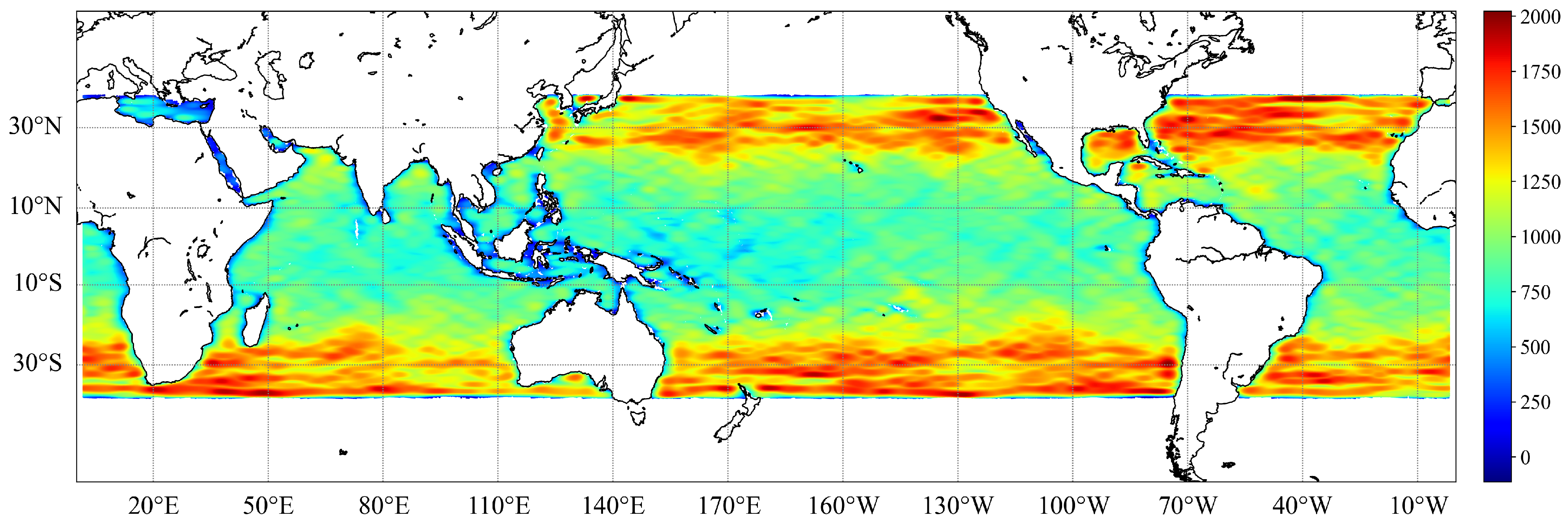
In this study, we used CCMP v02.0 (2017–2018) and v02.1.NRT (2019–2020) winds to assess the accuracy of the NOAA CyGNSS v1.1 product in global oceans. Here, we present the comparison of the CyGNSS/CCMP collocations during the period between May 2017 and December 2020. For illustrative purposes, Figure 2 shows the distribution of CyGNSS/CCMP collocations in global oceans. It can be seen that the area from 38 S to 38 N can be observed by CyGNSS due to the limitation of orbit [73]. The detectable area depends on the specular point of the associated global positioning system (GPS) transmitting satellite and CyGNSS receiving satellite [74]. The CCMP wind was regarded as the ground-truth observation, and was used to evaluate the performance of the NOAA CyGNSS wind product. CCMP wind was collocated with each CyGNSS specular point on the basis of the spatial and temporal collocation criteria. After the CyGNSS/CCMP collocating procedure, the total number of matchups was ∼7.45 million for May 2017–December 2020.
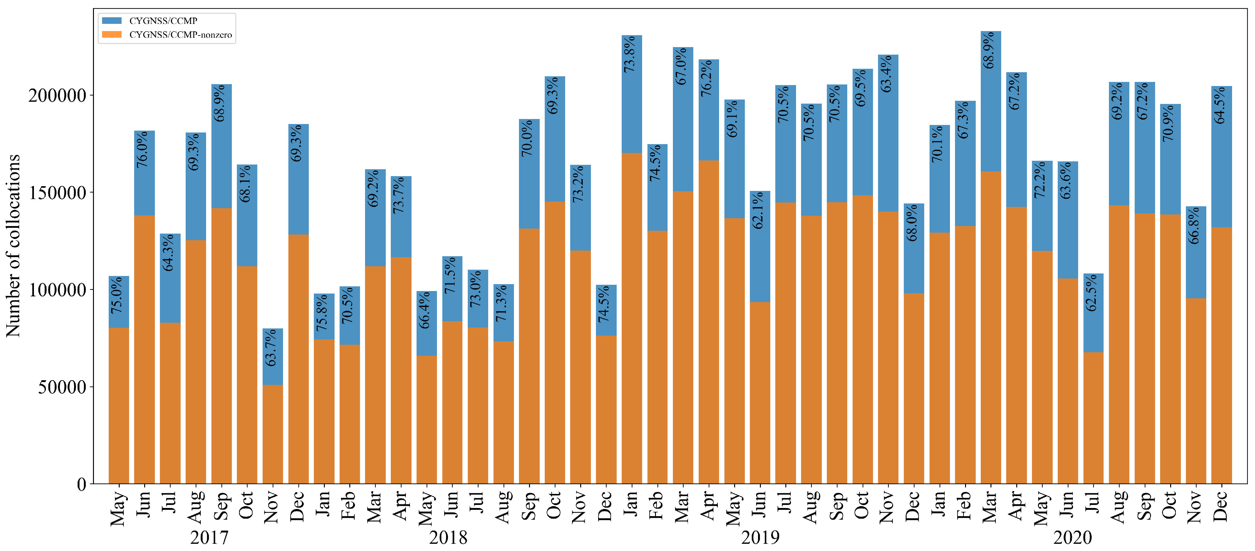
According to the flag named nobs from CCMP as mentioned above, CyGNSS/CCMP collocations were divided into CCMP-zero and CCMP-nonzero as shown in Figure 1. Figure 3 shows the volume of collocation data over the global oceans during the period between May 2017 and December 2020. The percentages per calendar month are displayed in each bar; the number of collocations is relatively lower in 2018 overall. The average percentage was 70.2% from 2017 to 2020. We found that the percentage of CCMP collocations with observation data flags was more than 60% in each month. This provide valuable collocations for us to assess the accuracy of the NOAA CyGNSS v1.1 product.
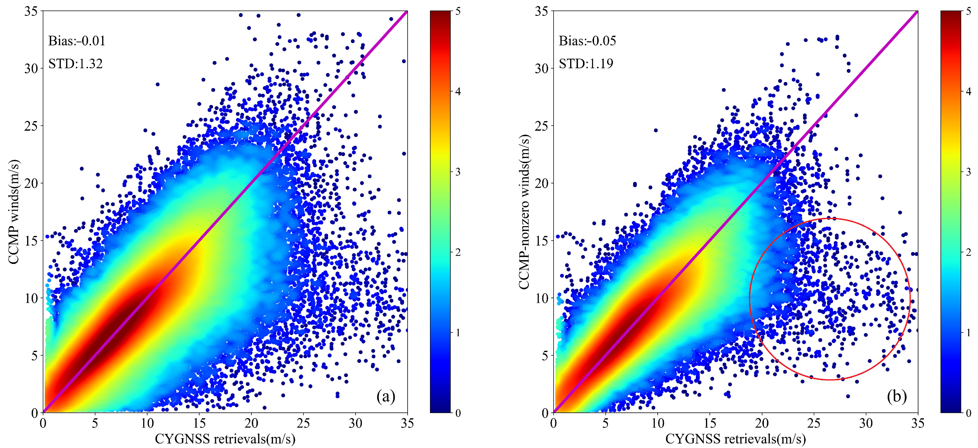
The overall performance of NOAA CyGNSS v1.1 compared with CCMP was evaluated in this study. Scatterplots of the wind speeds between CyGNSS and CCMP are presented in Figure 4, which show the global statistics for CyGNSS winds against the reference CCMP winds in the form of bias and SD. The average SDs of CyGNSS/CCMP and CyGNSS/CCMP-nonzero were 1.32 m/s and 1.19 m/s during the period between May 2017 and December 2020, respectively. This result is consistent with the analyses in [62], which reported that NOAA CyGNSS v1.1 against ECMWF achieved an SD of 1.19 m/s for wind speed.
Figure 4b shows that the highest density in the wind speed scatterplot (2–10 m/s) is very close to (magenta line), which is in agreement with the CCMP-nonzero wind speed. However, compared with CCMP winds, as shown in Figure 4a, the outliers still remained in the red circle, as shown in Figure 4b. The first reason may be the stability of the NOAA retrieval model, although a large amount of data was used for fitting. It could be possible that the outliers highlighted in Figure 4b are associated to low signal-to-noise ratio (SNR) levels (e.g., below 3 dB). The quality control may not be so strict, leading to some poor-quality data being used for inversion.
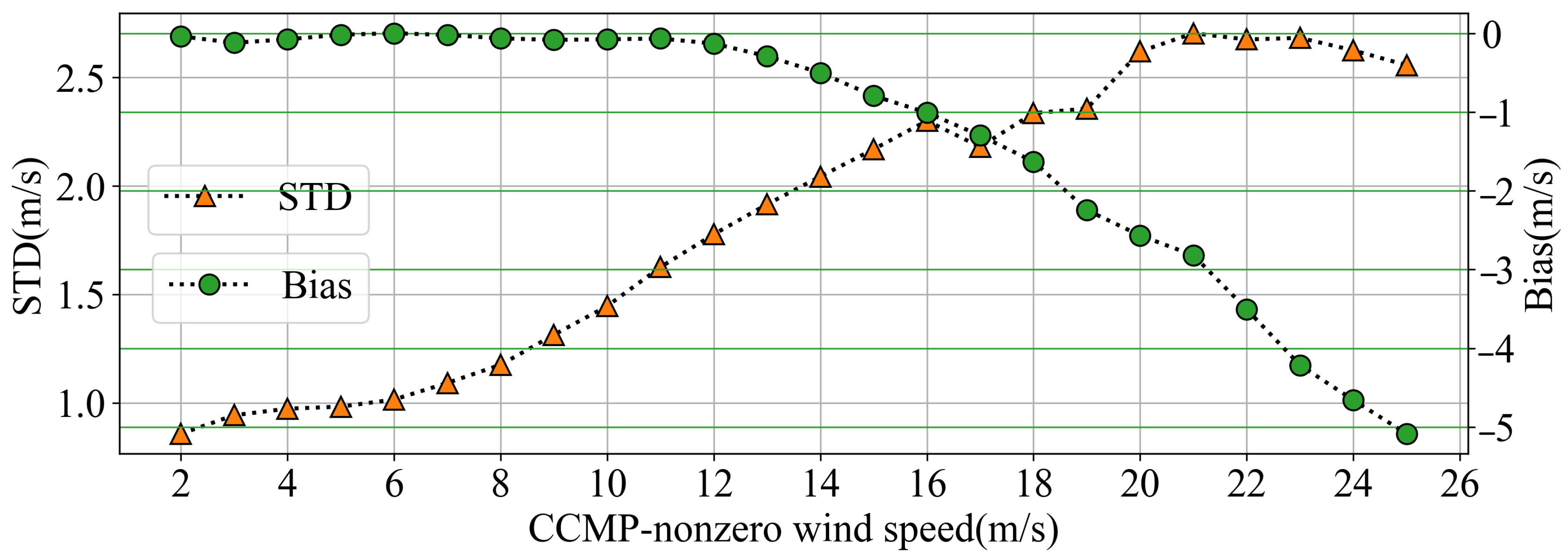
Figure 5 illustrates that the averaged metrics for wind speed ranging from 2 to 25 m/s were calculated according to the CCMP-nonzero wind speeds. The biases are close to zero, associated with small oscillations, and SDs are within 2 m/s in the range of 2 to 12 m/s, which shows that CyGNSS wind is very consistent with the CCMP-nonzero wind. However, average bias decreases with the increase in the CCMP-nonzero wind speed ranging from 12 to 25 m/s. We noted that the CyGNSS retrievals showed a large error for high wind speeds, which may be GNSS-R observations become relatively insensitive to high wind. Moreover, high wind is a very small proportion of the total, which produces instability when modeling the empirical model.
To analyze the features of the error distribution, the whole collocated set was divided into three subsets according to the magnitude of CCMP-nonzero wind speed. In the low wind speed regime, the wind speed is lower than 4 m/s; in the medium wind speed regime, the wind speed is between 4 and 20 m/s; wind speed greater than 20 m/s was classified as high wind speed. A total of ∼15.4% of the whole collocated set was classified as low wind speeds. The average bias was calculated by collocations between 0 and 4 m/s according to the magnitude of the CCMP-nonzero wind speed, which was m/s. Correspondingly, the average SD was 0.92 m/s. In the high speed regime (which included only 0.03% of the whole collocated set), Figure 5 shows a large negative mean deviation when the CCMP-nonzero wind speed is greater than 20 m/s. We clearly see that it decreases linearly from 0 to m/s with the increase in CCMP-nonzero wind speed. Lastly, in the medium wind speed range, the bias and SD on average were −0.06 m/s and 1.23 m/s, respectively, showing agreement with CCMP-nonzero and good performance. According to the overall accuracy (bias = −0.05 m/s and SD = 1.19 m/s), the sea surface wind speeds can be effectively provided by the NOAA CyGNSS product.
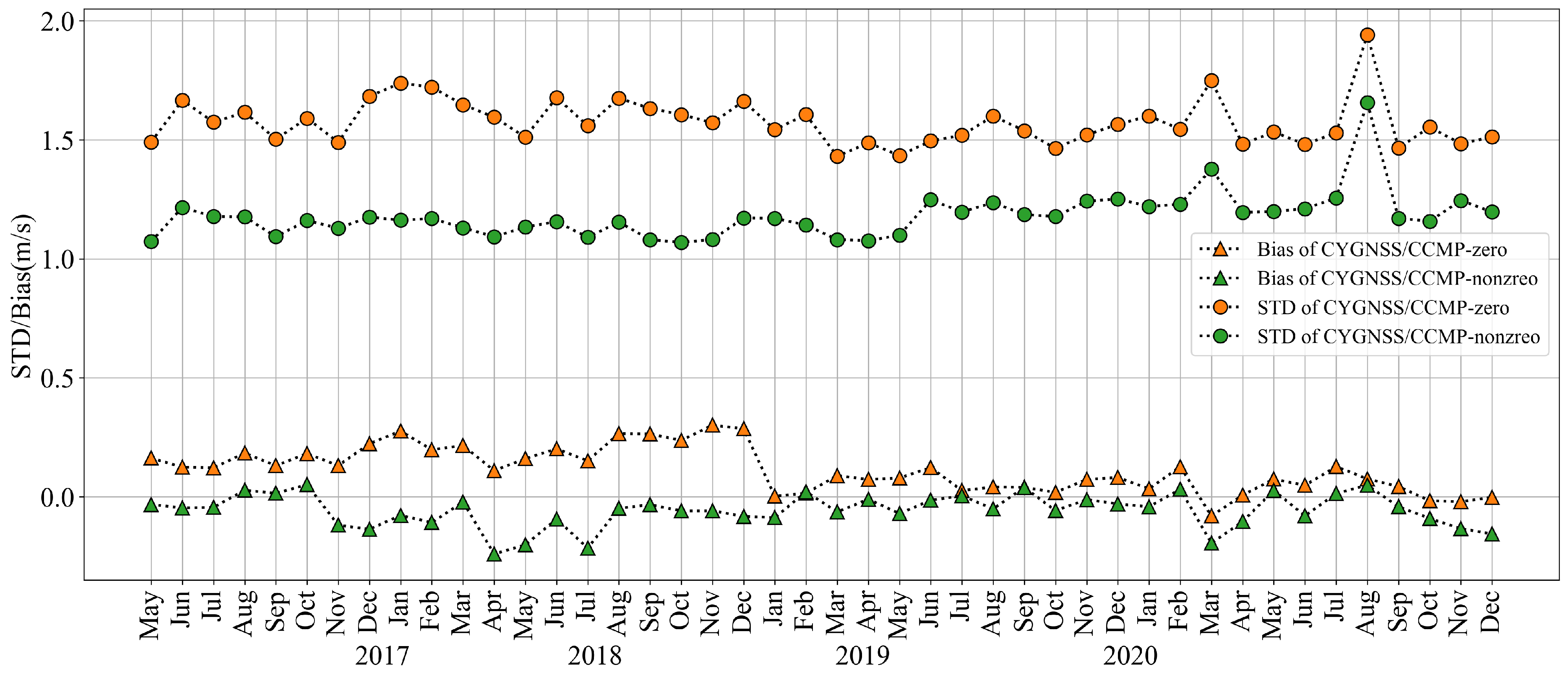
The performance of the NOAA CyGNSS product was also analyzed over the period between May 2017 and December 2020. Figure 6 provides the metrics of CyGNSS/CCMP collocations for each individual month. Compared with CCMP-zero winds, the CyGNSS winds had a persistent positive deviation of 0.10 m/s. The overall bias of CyGNSS/CCMP-nonzero was −0.05 m/s. However, the SD of CyGNSS/CCMP-zero was large at 1.57 m/s. The comparison shows that NOAA CyGNSS winds are in good agreement with CCMP-nonzero winds. In addition, from Figure 6, the monthly SDs of CyGNSS/CCMP-zero were all bigger than those of CyGNSS/CCMP-nonzero from 2017 to 2020. The monthly bias of CyGNSS/CCMP-zero in 2018 was higher than in other years. On the contrary, the monthly bias of CyGNSS/CCMP-nonzero was lower. Subsequently, both monthly biases appear to have stabilized in 2019 and 2020. The time series of bias shows a discrepancy in the earlier period. There may be two reasons for this finding: One is that the block IIR-M and most IIF GPS experienced power flex events in 2018. As a result, the CyGNSS observations estimated from these are questionable. So, the performance was degraded. Another reason is that both CCMP v02.0 (2017–2018) and CCMP v02.1.NRT (2019–2020) products were used to evaluate the accuracy of the CyGNSS sea surface wind speed in global oceans. There will be a difference between the two products.
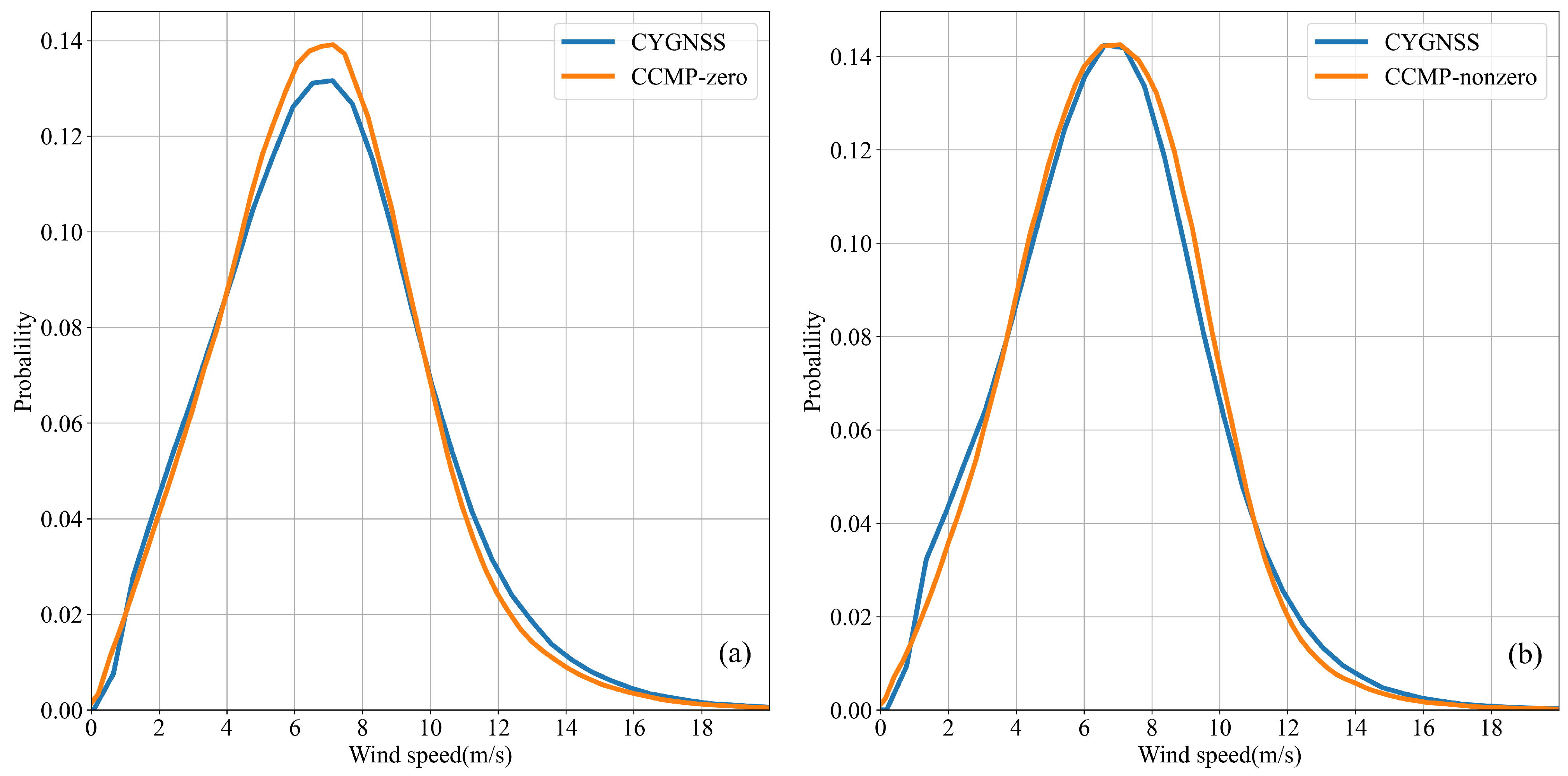
Figure 7 presents the probability density function (PDF) of the CyGNSS winds with respect to CCMP-zero and CCMP-nonzero in the range of 0 to 20 m/s during the period between May 2017 and December 2020. By comparing the two subfigures in Figure 7, the CCMP-zero winds are shown to be slightly higher than NOAA CyGNSS winds at moderate wind speeds. Figure 7b indicates the PDF of CyGNSS winds coincides with that of CCMP-nonzero winds. The performance of CyGNSS winds relative to CCMP-nonzero ones is significantly better, with a SD of 1.19 m/s on average. In general, the CyGNSS winds are in agreement with CCMP-nonzero winds. The NOAA CyGNSS v1.1 product has approximately the same wind speeds with CCMP-nonzero wind: the PDF curves almost coincide, consistent with the result in Figure 7b.
3.2. Global Statistics of CyGNSS/CCMP-Nonzero
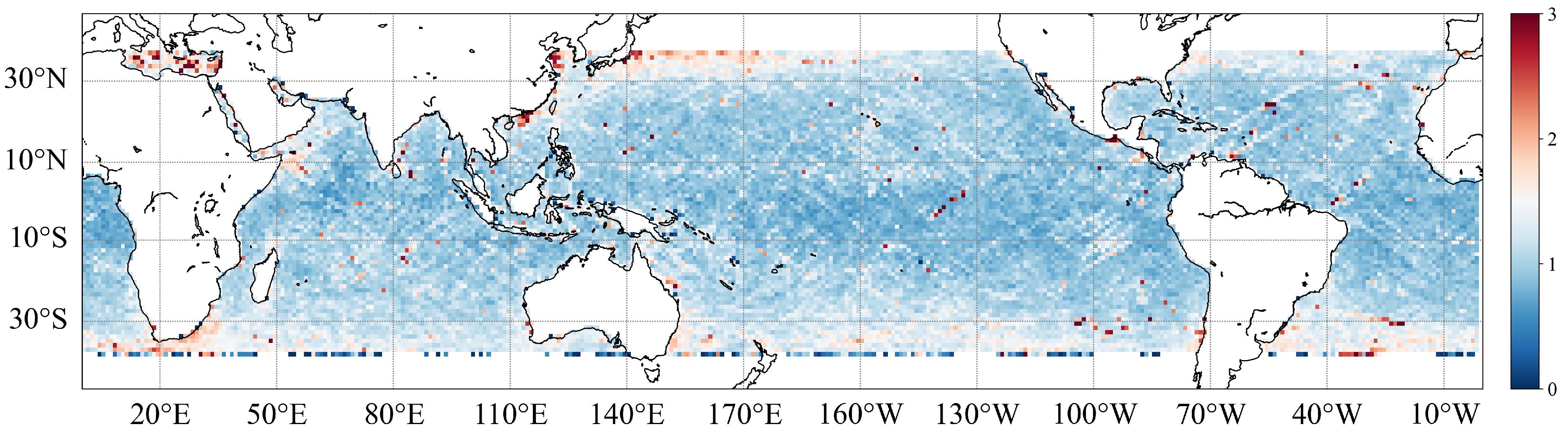
The geographical distribution characteristics of CyGNSS in terms of bias and SD were investigated. CyGNSS/CCMP-nonzero collocations were divided on a regular geographical grid of 1 by 1. The relevant information of the re-gridded map method is described in Section 2.4. A global map with spatial resolution of 1 gridded SD was constructed as shown in Figure 8, which illustrates the SD of NOAA CyGNSS values compared with CCMP-nonzero values in the global oceans. A large part of the global 1 gridded map in SD is blue, which indicates that NOAA CyGNSS winds well-agree with CCMP-nonzero ones. Islands have little influence on retrieval accuracy, e.g., near Malaysia and the Philippines. However, we found that large SDs occur in the Mediterranean Sea, the southern coast of Africa, and the east coast of China. These errors should be further investigated.
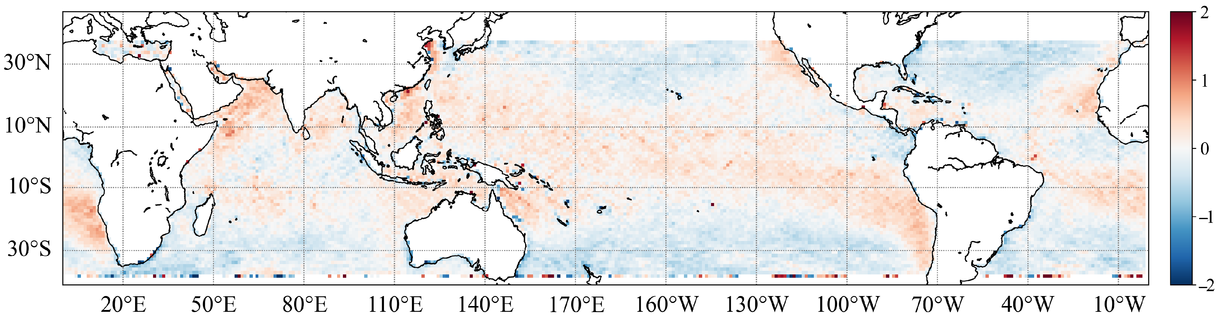
Figure 9 shows the distribution of the wind speed bias between CyGNSS and CCMP-nonzero. We found that negative deviation mainly appears at high latitudes in both hemispheres, and especially in the southern hemisphere. The bias is obvious when the latitude exceeds 30 S. The negative deviation of the northern hemisphere mainly occurs in the Northern Pacific and the north center of the Atlantic Ocean, especially along the east coast of the United States and Australia. However, positive deviations appear in the China Sea, Arabian Sea, and the west of Africa and South America. The red density points reveal where CyGNSS winds overestimate CCMP-nonzero winds for every ocean between 20 S and 20 N, as shown in Figure 9. In particular, the quality of CyGNSS winds in the China Sea is not ideal, with a large SD and a positive bias. In addition, as shown in Figure 8, the map of the wind speed SD between CyGNSS and CCMP-nonzero shows the high accuracy, and the wind speed bias has a small deviation in the adjacent sea region to Malaysia and the Philippines.
Sampling points with poor inversion accuracy were mostly distributed along the coast, as shown in Figure 8 and Figure 9. The wind speed retrieval performance of NOAA CyGNSS in coastal regions was also analyzed. Coastal winds (within 50 km from the coastline) of CyGNSS/CCMP-nonzero were determined using the global coastline dataset (http://www.soest.hawaii.edu/pwessel/gshhg/, (accessed on 31 January 2021)) [75]. The accuracy of CyGNSS winds in coastal regions was evaluated: a bias of −0.19 m/s and an SD of 1.45 m/s were obtained. This performance is not as good as the overall performance. The main reason for this degradation is that GMFs are established by global winds, so these are inapplicable of retrieving coastal winds. The wind field from the coastal regions is strongly affected by shoreline and shallow water, which increase the difficulty of retrieval of winds by GMFs.
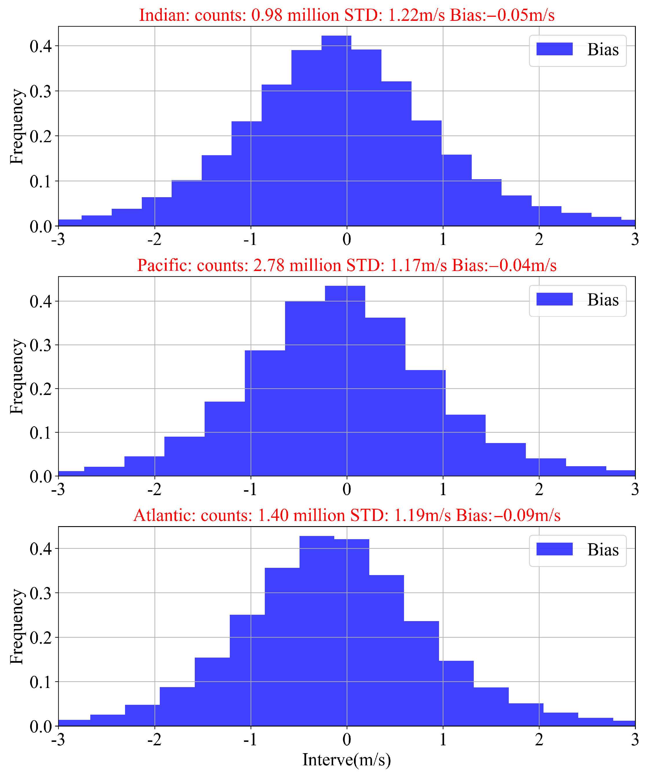
The counts, SD, and bias of NOAA CyGNSS values with respect to CCMP-nonzero ones over the tropical Pacific, Atlantic, and Indian Oceans were investigated and analyzed. The number of collocations in each ocean depends on its size. The accuracy evaluation of the Pacific, Atlantic, and Indian Oceans is shown in Figure 10. The results showed that the difference in the Pacific, Atlantic, and Indian Oceans was non-significant in bias. The mean deviation of the Indian Ocean was m/s with an SD of 1.22 m/s; the mean deviation of the Pacific Ocean was −0.04 m/s with an SD of 1.17 m/s; the mean deviation of the Atlantic Ocean was −0.09 m/s with an SD of 1.19 m/s. Figure 10 also shows the histogram of NOAA CyGNSS winds relative to CCMP-nonzero ones over the tropical Pacific, Atlantic, and Indian Oceans. We see this clearly in Figure 10, where the biases of the Pacific, Atlantic, and Indian Oceans are concentrated between −3 and 3 m/s. The mean deviations for each ocean are negative, which demonstrates the overall underestimation in CyGNSS wind speed over the tropical Pacific, Atlantic ,and Indian Oceans. The performance in the Atlantic Ocean is the worst. The number of collocations can also affect the accuracy. Figure 10 provides the counts of the tropical Pacific, Atlantic, and Indian Oceans. The more likely reason for this finding is that this difference in the three oceans may be determined by their own wind field characteristics, such as the occurrence and geographical distribution of high wind events. Certainly, these differences could also be due to the performance of the CCMP product in different ocean basins. The geographical dependence of the wind speed retrieval error should be further investigated.
4. Discussion
The performance verification of wind speed retrieval is a key criterion for operational products. At present, according to our comparison result, the NOAA CyGNSS v1.1 product meets the design performance requirements for wind speed accuracy across the wind speed range from 2 to 20 m/s at a 25 km resolution. The results described in this paper are consistent with those described in [68], whereas the performance in the high wind regime troubles. CyGNSS always underestimates high wind speeds. Maybe GNSS-R observations are relatively insensitive to high wind. Moreover, high wind represents a very small proportion of the total, which poses difficulties for modeling empirical models. So, the retrieval performance at high wind speeds should be further investigated.
As a result of the aforementioned comparison and analysis, the overall performance consistency and reliability were determined. However, abnormal geographical anomalies were found. From Figure 9, we found that negative deviation mainly appears in high latitude areas in both hemispheres. Positive deviations appear in the China Sea, Arabian Sea, and the west of Africa and South America. In particular, a large error (both SD and bias) was found in the coastal areas of China. The aforementioned phenomenon occurred in the previous version as well. Both NASA v2.1 and NOAA v1.0 wind products show large errors relative to ECMWF reanalysis data in the coastal areas of China, which was presented in a technical report [76]. A recent study showed that the overall performance of CyGNSS v1.1 against ECMWF also displays this phenomenon. Said et al. discussed and explained this phenomenon, which may be caused by radio frequency interference [68].
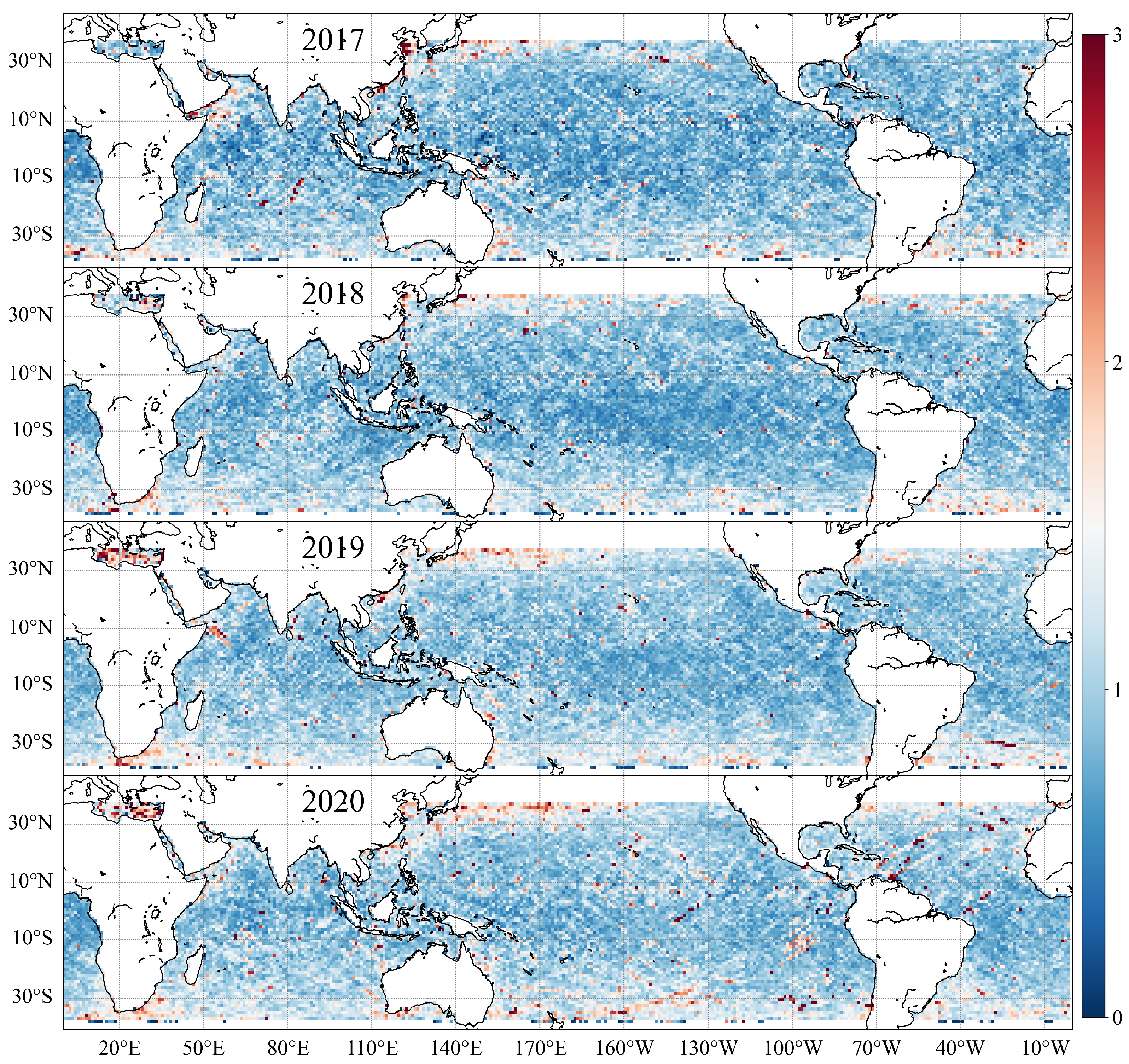
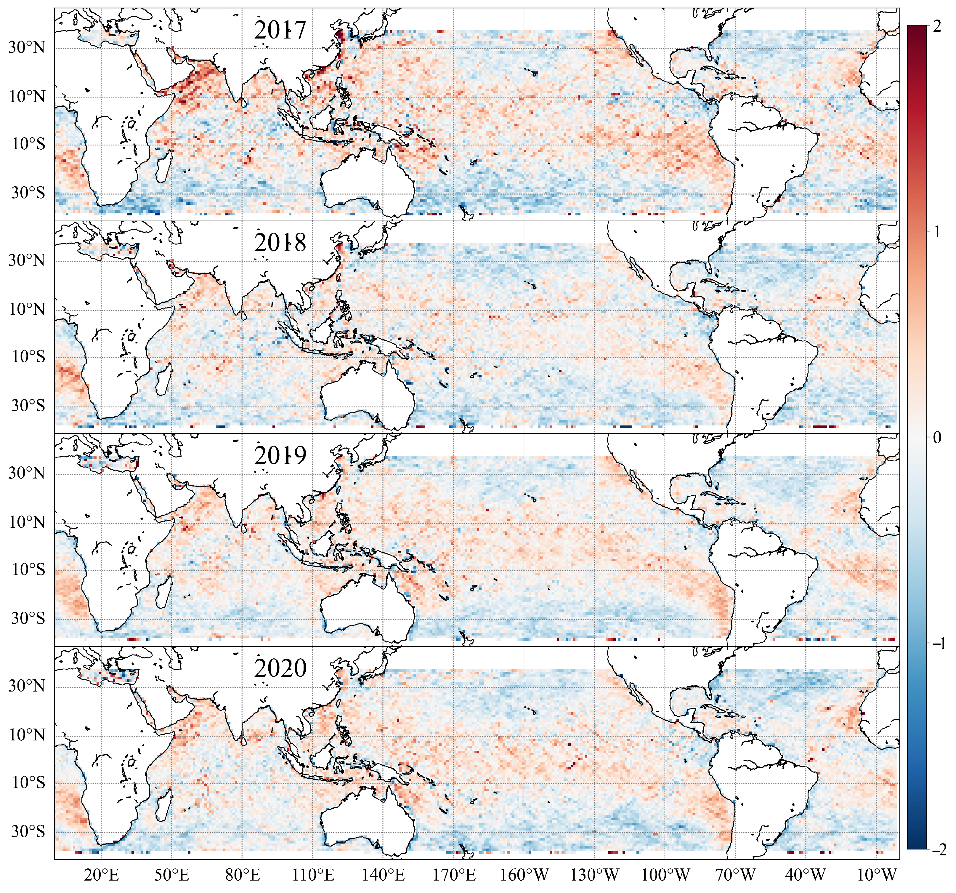
To further determine whether the geographical anomalies are temporally temporary, the interannual variations in the SD and wind speed bias between CyGNSS and CCMP-nonzero were investigated, as shown in Figure 11 and Figure 12. The SD of CyGNSS along the China coast has been improved over time, with the SD (red color) gradually becoming small (white color). Unfortunately, the accuracy remains poor (red color) in the Mediterranean region and the middle-upper region of the Pacific Ocean. The distribution of SD between CyGNSS and CCMP-nonzero in other regions is similar to the average SD in 2018–2020. Figure 12 shows that there was no significant difference in the spatial distribution of the wind speed bias from 2018 to 2020. Note that the global distribution of the wind speed bias in 2017 showed larger errors occurred in the China Sea and Arabian Sea. This is consistent with the result shown in Figure 9. The improvement in the wind speed bias is not as obvious as that in SD over time. Negative deviations mainly appeared in high latitudes in 2017–2020, as shown in Figure 12, especially in the southern hemisphere. This basically confirms that the geographical anomaly is not temporary. The specific reasons may be related to the distribution of wind speed and the retrieval method, which will not be discussed in detail here.
5. Conclusions
This paper presented a preliminary assessment of the quality of remotely sensed wind speed measurements produced by NOAA CyGNSS. The performance of CyGNSS v1.1 winds between 38 S and 38 N was investigated. Compared with CCMP-zero and nonzero collocations, we found that NOAA CyGNSS winds agree well with CCMP-nonzero winds that combine in situ sea surface wind speed observations. A bias of nearly −0.05 m/s and an SD of 1.19 m/s were obtained against CCMP-nonzero winds during the period from May 2017 to December 2020. Further analysis indicated that the wind retrievals substantially degrade for wind speeds greater than 20 m/s and are most accurate in the 2–12 m/s wind speed regime. Furthermore, we systematically compared the NOAA CyGNSS and CCMP-nonzero winds on spatial and temporal scales. The results of time series analysis illustrated that the CyGNSS wind is consistent and reliable generally. Additionally, the geographical distribution characteristics of the CyGNSS winds were investigated using the interannual variations in the SD and wind speed bias. We found that the geographical anomaly in bias was not temporary. Moreover, evaluation of coastal CyGNSS winds (within 50 km from the coastline) showed that its performance was not as good as the overall performance.
The metrics of CyGNSS/CCMP-nonzero were calculated in the Pacific, Atlantic, and Indian Oceans. We found the NOAA CyGNSS wind in the Pacific Ocean performed better than in the Atlantic and Indian Oceans. It can be seen from the metrics of three oceans that the difference in the three oceans may be determined by their own wind field characteristics. Overall, the quantitative comparison in this study indicates that the CyGNSS wind v1.1 product provides good and stable performance over time. The sea surface wind product acquired from the CyGNSS mission in 2017–2020 is valuable for practical use.
Author Contributions
X.L. carried out the evaluations and analysis, and wrote the original draft; D.Y. and J.Y. designed the schemes and led the main work in this study; W.L. and G.Z. analyzed the data and offered many valuable comments and considerations; G.H. provided several opinions and constructive suggestions and discussions. All authors have read and agreed to the published version of the manuscript.
Funding
This research was funded by the National Key Research and Development Plan under grant Nos. 2016YFC1401003 and 2017YFB050802; the National Natural Science Foundation of China under grant Nos. 41774028 and 41676167; the Zhejiang Provincial Natural Science Foundation of China, under grant No. LR21D060002; the Key R&D Project of Shandong Province under grant No. 2019JZZY010102; the Project of State Key Laboratory of Satellite Ocean Environment Dynamics, Second Institute of Oceanography, under grant No. SOEDZZ2003; and the Strategic Priority Research Program of the Chinese Academy of Sciences under grant Nos. XDA19090103 and XDB42000000. This work of W.L. was supported in part by the Spanish Ministry of Economy and Competitiveness and EU/FEDER (ESP2015-70014-C2-2-R) and the Ramón y Cajal Program (RYC2019-027000-I). This work was also supported by ESA-MOST Dragon-4 project (id. 32249) and Dragon-5 project (id. 58009).
Acknowledgments
The authors are grateful to the NOAA ocean surface winds team for making the CYGNSS L2 data publicly available through the Center for Satellite Application and Research (STAR), NESDIS/NOAA.
Conflicts of Interest
The authors declare no conflict of interest.
References
- Bentamy, A.; Queffeulou, P.; Quilfen, Y.; Katsaros, K. Ocean surface wind fields estimated from satellite active and passive microwave instruments. IEEE Trans. Geosci. Remote Sens. 1999, 37, 2469–2486. [Google Scholar] [CrossRef]
- D’Asaro, E.A. The Energy Flux from the Wind to Near-Inertial Motions in the Surface Mixed Layer. J. Phys.Oceanogr. 1985, 15, 1043–1059. [Google Scholar] [CrossRef] [Green Version]
- Christiansen, M.B.; Koch, W.; Horstmann, J.; Hasager, C.B.; Nielsen, M. Wind resource assessment from C-band SAR. Remote. Sens. Environ. 2006, 105, 68–81. [Google Scholar] [CrossRef] [Green Version]
- Tang, R.; Liu, D.; Han, G.; Ma, Z.; De Young, B. Reconstructed Wind Fields from Multi-Satellite Observations. Remote. Sens. 2014, 6, 2898–2911. [Google Scholar] [CrossRef] [Green Version]
- Hu, T.; Li, Y.; Li, Y.; Wu, Y.; Zhang, D. Retrieval of Sea Surface Wind Fields Using Multi-Source Remote Sensing Data. Remote. Sens. 2020, 12, 1482. [Google Scholar] [CrossRef]
- Atlas, R.; Hoffman, R.N.; Leidner, S.M.; Sienkiewicz, J.; Yu, T.W.; Bloom, S.C.; Brin, E.; Ardizzone, J.; Terry, J.; Bungato, D.A. The Effects of Marine Winds from Scatterometer Data on Weather Analysis and Forecasting. Bull. Am. Meteorol. Soc. 2010, 82, 1965–1990. [Google Scholar] [CrossRef] [Green Version]
- Xing, J.; Shi, J.; Lei, Y.; Huang, X.Y.; Liu, Z. Evaluation of HY-2A scatterometer wind vectors using data from buoys, ERA-interim and ASCAT during 2012–2014. Remote. Sens. 2016, 8, 390. [Google Scholar] [CrossRef] [Green Version]
- Zhou, L.; Zheng, G.; Li, X.; Yang, J.; Lou, X. An Improved Local Gradient Method for Sea Surface Wind Direction Retrieval from SAR Imagery. Remote Sens. 2017, 9, 671. [Google Scholar] [CrossRef] [Green Version]
- Varvayanni, M.; Bartzis, J.; Catsaros, N.; Graziani, G.; Deligiannis, P. Numerical simulation of daytime mesoscale flow over highly complex terrain: Alps case. Atmos. Environ. 1998, 32, 1301–1316. [Google Scholar] [CrossRef]
- Woiceshyn, P.M.; Wurtele, M.G.; Boggs, D.H.; Mcgoldrick, L.F.; Peteherych, S. The necessity for a new parametrisation of an empirical model for wind/ocean scatterometry. J. Geophys. Res. Atmos. 1986, 91, 2273–2288. [Google Scholar] [CrossRef]
- Chelton, D.B.; Wentz, F.J. Further Development of an Improved Altimeter Wind Speed Algorithm. J. Geophys. Res. Atmos. 1987, 91, 14250–14260. [Google Scholar] [CrossRef]
- Goodberlet, M.A.; Swift, C.T.; Wilkerson, J.C. Remote sensing of ocean surface winds with the special sensor microwave/imager. J. Geophys. Res. Oceans 1989, 94, 14547–14555. [Google Scholar] [CrossRef]
- Quilfen, Y.; Cavanie, A. A High Precision Wind Algorithm For The Ers1 Scatterometer Furthermore, Its Validation. In Proceedings of the 11th Annual International Geoscience and Remote Sensing Symposium, Espoo, Finland, 3–6 June 1991; IEEE: Espoo, Finland, 1991. [Google Scholar]
- Flett, D.G.; Wilson, K.J.; Vachon, P.W.; Hopper, J.F. Wind information for marine weather forecasting from RADARSAT-1 synthetic aperture radar data: Initial results from the “Marine winds from SAR” demonstration project. Can. J. Remote Sens. 2002, 28, 490–497. [Google Scholar] [CrossRef]
- Jochen, H.; Wolfgang, K.; Susanne, L.; Rasmus, T. Ocean winds from RADARSAT-1 ScanSAR. Can. J. Remote Sens. 2002, 28, 524–533. [Google Scholar]
- Du, Y.; Vachon, P.W.; Wolfe, J. Wind direction estimation from SAR images of the ocean using wavelet analysis. Can. J. Remote Sens. 2002, 28, 498–509. [Google Scholar] [CrossRef]
- Vachon, P.W.; Wolfe, J.; Hawkins, R.K. Comparison of C-band wind retrieval model functions with airborne multipolarization SAR data. Can. J. Remote Sens. 2004, 30, 462–469. [Google Scholar] [CrossRef]
- Montuori, A.; Ricchi, A.; Benassai, G.; Migliaccio, M. Sea Wave Numerical Simulations and Verification in Tyrrhenian Coastal Area with X-Band Cosmo-Skymed SAR Data. In Proceedings of the ESA, SOLAS & EGU Joint Conference Earth Observation for Ocean-Atmosphere Interactions Science, Frascati, Italy, 29 November–2 December 2011. [Google Scholar]
- Benassai, G.; Migliaccio, M.; Montuori, A.; Ricchi, A. SWAN wave simulations in the Southern Thyrrenian Sea with COSMO SKY-MED SAR data. In Proceedings of the EGU General Assembly, Vienna, Austria, 22–27 April 2012. [Google Scholar]
- Bourassa, M.A.; Meissner, T.; Cerovecki, I.; Chang, P.S.; Dong, X.; De Chiara, G.; Donlon, C.; Dukhovskoy, D.S.; Elya, J.; Fore, A.; et al. Remotely Sensed Winds and Wind Stresses for Marine Forecasting and Ocean Modeling. Front. Mar. Sci. 2019, 6, 443. [Google Scholar] [CrossRef] [Green Version]
- Hasager, C.; Sjöholm, M. (Eds.) Remote Sensing of Atmospheric Conditions for Wind Energy Applications; Remote Sensing, MDPI Books; MDPI: Basel, Switzerland, 2019. [Google Scholar] [CrossRef] [Green Version]
- McCollum, J.R. Next generation of NOAA/NESDIS TMI, SSM/I, and AMSR-E microwave land rainfall algorithms. J. Geophys. Res. Atmos. 2003, 108, 8382. [Google Scholar] [CrossRef]
- Surussavadee, C.; Staelin, D.H.; Chadarong, V.; Mclaughlin, D.; Entekhabi, D. Comparison of NOWRAD, AMSU, AMSR-E, TMI, and SSM/I surface precipitation rate Retrievals over the united states great plains. In Proceedings of the 2007 IEEE International Geoscience and Remote Sensing Symposium, Barcelona, Spain, 23–27 July 2007; IEEE: New York, NY, USA, 2008. [Google Scholar]
- Dee, D.P.; Uppala, S.M.; Simmons, A.J.; Berrisford, P.; Poli, P.; Kobayashi, S.; Vitart, F. The ERA-Interim reanalysis: Configuration and performance of the data assimilation system. Q. J. R. Meteorol. Soc. 2011, 137, 553–597. [Google Scholar] [CrossRef]
- Saha, S.E.A. The NCEP Climate Forecast System Version 2. J. Clim. 2012, 27, 2185–2208. [Google Scholar] [CrossRef]
- Atlas, R.; Hoffman, R.N.; Ardizzone, J.; Leidner, S.M.; Jusem, J.C.; Smith, D.K.; Gombos, D. A Cross-calibrated, Multiplatform Ocean Surface Wind Velocity Product for Meteorological and Oceanographic Applications. Bull. Am. Meteorol. Soc. 2011, 92, 157–174. [Google Scholar] [CrossRef]
- Chen, J.; Weisberg, R.H.; Liu, Y.; Zheng, L. The Tampa Bay Coastal Ocean Model Performance for Hurricane Irma. Mar. Technol. Soc. J. 2018, 52, 33–42. [Google Scholar] [CrossRef]
- Mayer, D.A.; Weisberg, R.H.; Zheng, L.; Liu, Y. Winds on the West Florida Shelf: Regional comparisons between observations and model estimates. J. Geophys. Res. Oceans 2017, 122, 834–846. [Google Scholar] [CrossRef] [Green Version]
- Martín-Neira, M. A Passive Reflectometry and Interferometry System (PARIS): Application to ocean altimetry. ESA J. 1993, 17, 331–355. [Google Scholar]
- Clarizia, M.P.; Ruf, C.S. Wind Speed Retrieval Algorithm for the Cyclone Global Navigation Satellite System (CYGNSS) Mission. IEEE Trans. Geosci. Remote Sens. 2016, 54, 4419–4432. [Google Scholar] [CrossRef]
- Ruf, C.S.; Balasubramaniam, R. Development of the CYGNSS Geophysical Model Function for Wind Speed. IEEE J. Sel. Top. Appl. Earth Observ. Remote Sens. 2019, 12, 66–77. [Google Scholar] [CrossRef]
- Soulat, F. Sea state monitoring using coastal GNSS-R. Geophys. Res. Lett. 2004, 31, 133–147. [Google Scholar] [CrossRef] [Green Version]
- Roggenbuck, O.; Reinking, J.; Lambertus, T. Determination of Significant Wave Heights Using Damping Coefficients of Attenuated GNSS SNR Data from Static and Kinematic Observations. Remote Sens. 2019, 11, 409. [Google Scholar] [CrossRef] [Green Version]
- Alonso-Arroyo, A.; Zavorotny, V.U.; Camps, A. Sea Ice Detection Using U.K. TDS-1 GNSS-R Data. IEEE Trans. Geosci. Remote Sens. 2017, 55, 4989–5001. [Google Scholar] [CrossRef] [Green Version]
- Yan, Q.; Huang, W. Sea Ice Sensing From GNSS-R Data Using Convolutional Neural Networks. IEEE Geosci. Remote Sens. Lett. 2018, 15, 1510–1514. [Google Scholar] [CrossRef]
- Li, W.; Cardellach, E.; Fabra, F.; Rius, A.; Ribó, S.; Martín-Neira, M. First spaceborne phase altimetry over sea ice using TechDemoSat-1 GNSS-R signals. Geophys. Res. Lett. 2017, 44, 8369–8376. [Google Scholar] [CrossRef]
- Hu, C.; Benson, C.R.; Qiao, L.; Rizos, C. The Validation of the Weight Function in the Leading-Edge-Derivative Path Delay Estimator for Space-Based GNSS-R Altimetry. IEEE Trans. Geosci. Remote Sens. 2020, 58, 6243–6254. [Google Scholar] [CrossRef]
- Tabibi, S.; Geremia-Nievinski, F.; Francis, O.; van Dam, T. Tidal analysis of GNSS reflectometry applied for coastal sea level sensing in Antarctica and Greenland. Remote Sens. Environ. 2020, 248, 111959. [Google Scholar] [CrossRef]
- Schmugge, T.; Jackson, T.J. Mapping surface soil moisture with microwave radiometers. Meteorol. Atmos. Phys. 1994, 54, 213–223. [Google Scholar] [CrossRef]
- Rodriguez-Alvarez, N.; Bosch-Lluis, X.; Camps, A.; Vall-Llossera, M.; Valencia, E.; Marchan-Hernandez, J.F.; Ramos-Perez, I. Soil Moisture Retrieval Using GNSS-R Techniques: Experimental Results Over a Bare Soil Field. IEEE Trans. Geosci. Remote Sens. 2009, 47, 3616–3624. [Google Scholar] [CrossRef]
- Martín-Neira, M.; Caparrini, M.; Font-Rossello, J.; Lannelongue, S.; Vallmitjana, C.S. The PARIS Concept: An Experimental Demonstration of Sea Surface Altimetry Using GPS Reflected Signals. IEEE Trans. Geosci. Remote Sens. 2001, 39, 142–150. [Google Scholar] [CrossRef] [Green Version]
- Martín-Neira, F.; Camps, A.; Martin-Neira, M.; D’Addio, S.; Park, H. Significant wave height retrieval based on the effective number of incoherent averages. In Proceedings of the 2015 IEEE International Geoscience and Remote Sensing Symposium (IGARSS), Milan, Italy, 26–31 July 2015; IEEE: New York, NY, USA, 2015; pp. 3634–3637. [Google Scholar]
- Zavorotny, V.U.; Voronovich, A.G. Scattering of GPS signals from the ocean with wind remote sensing application. IEEE Trans. Geosci. Remote Sens. 2000, 38, 951–964. [Google Scholar] [CrossRef] [Green Version]
- Komjathy, A.; Zavorotny, V.U.; Axelrad, P.; Born, G.H.; Garrison, J.L. GPS Signal Scattering from Sea Surface: Wind Speed Retrieval Using Experimental Data and Theoretical Model. Remote Sens. Environ. 2000, 73, 162–174. [Google Scholar] [CrossRef]
- Cardellach, E.; Fabra, F.; Nogués-Correig, O.; Oliveras, S.; Ribó, S.; Rius, A. GNSS-R ground-based and airborne campaigns for ocean, land, ice, and snow techniques: Application to the GOLD-RTR data sets. Radio Sci. 2011, 46. [Google Scholar] [CrossRef] [Green Version]
- Lowe, S.T.; Zuffada, C.; Chao, Y.; Kroger, P.; Young, L.E.; Labrecque, J.L. 5-cm-Precision aircraft ocean altimetry using GPS reflections. Geophys. Res. Lett. 2002, 29, 1375. [Google Scholar] [CrossRef] [Green Version]
- Cardellach, E.; Rius, A.; Martin-Neira, M.; Fabra, F.; Nogues-Correig, O.; Ribo, S.; Kainulainen, J.; Camps, A.; D’Addio, S. Consolidating the Precision of Interferometric GNSS-R Ocean Altimetry Using Airborne Experimental Data. IEEE Trans. Geosci. Remote Sens. 2014, 52, 4992–5004. [Google Scholar] [CrossRef]
- Egido, A.; Paloscia, S.; Motte, E.; Guerriero, L.; Pierdicca, N.; Caparrini, M.; Santi, E.; Fontanelli, G.; Floury, N. Airborne GNSS-R Polarimetric Measurements for Soil Moisture and Above-Ground Biomass Estimation. IEEE J. Sel. Top. Appl. Earth Observ. Remote Sens. 2017, 7, 1522–1532. [Google Scholar] [CrossRef]
- Lowe, S.T.; Labrecque, J.L.; Zuffada, C.; Romans, L.J.; Young, L.E.; Hajj, G.A. First spaceborne observation of an Earth-reflected GPS signal. Radio Sci. 2016, 37. [Google Scholar] [CrossRef]
- Gleason, S.; Hodgart, S.; Sun, Y.; Gommenginger, C.; Mackin, S.; Adjrad, M.; Unwin, M. Detection and Processing of bistatically reflected GPS signals from low Earth orbit for the purpose of ocean remote sensing. IEEE Trans. Geosci. Remote Sens. 2005, 43, 1229–1241. [Google Scholar] [CrossRef] [Green Version]
- Foti, G.; Gommenginger, C.; Jales, P.; Unwin, M.; Rosello, J. Spaceborne GNSS reflectometry for ocean winds: First results from the UK TechDemoSat-1 mission. Geophys. Res. Lett. 2015, 42, 5435–5441. [Google Scholar] [CrossRef] [Green Version]
- Asgarimehr, M.; Wickert, J.; Reich, S. TDS-1 GNSS Reflectometry: Development and Validation of Forward Scattering Winds. IEEE J. Sel. Top. Appl. Earth Observ. Remote Sens. 2018, 11, 4534–4541. [Google Scholar] [CrossRef]
- Soisuvarn, S.; Jelenak, Z.; Said, F.; Chang, P.S.; Egido, A. The GNSS Reflectometry Response to the Ocean Surface Winds and Waves. IEEE J. Sel. Top. Appl. Earth Observ. Remote Sens. 2017, 9, 4678–4699. [Google Scholar] [CrossRef]
- Foti, G.; Gommenginger, C.; Unwin, M.; Jales, P.; Tye, J.; Roselló, J. An Assessment of Non-geophysical Effects in Spaceborne GNSS Reflectometry Data From the UK TechDemoSat-1 Mission. IEEE J. Sel. Top. Appl. Earth Observ. Remote Sens. 2019, 10, 3418–3429. [Google Scholar] [CrossRef] [Green Version]
- Hammond, M.L.; Foti, G.; Gommenginger, C.; Srokosz, M. Temporal variability of GNSS-Reflectometry ocean wind speed retrieval performance during the UK TechDemoSat-1 mission. Remote Sens. Environ. 2020, 242, 111744. [Google Scholar] [CrossRef]
- Ruf, C.; Twigg, D. Level 1 and 2 Trackwise Corrected Climate Data Record Algorithm Theoretical Basis Document. 2020. Available online: https://clasp-research.engin.umich.edu/missions/cygnss/reference/148-0389 (accessed on 2 February 2021).
- Jing, C.; Niu, X.; Duan, C.; Lu, F.; Yang, X. Sea Surface Wind Speed Retrieval from the First Chinese GNSS-R Mission: Technique and Preliminary Results. Remote Sens. 2019, 11, 3013. [Google Scholar] [CrossRef] [Green Version]
- Clarizia, M.P.; Ruf, C.S.; Jales, P.; Gommenginger, C. Spaceborne GNSS-R Minimum Variance Wind Speed Estimator. IEEE Trans. Geosci. Remote Sens. 2014, 52, 6829–6843. [Google Scholar] [CrossRef]
- Clarizia, M.P.; Ruf, C.S.; Gleason, S.; Balasubramaniam, R.; Mckague, D. Generation of CYGNSS level 2 wind speed data products. In Proceedings of the 2017 IEEE International Geoscience and Remote Sensing Symposium (IGARSS), FortWorth, TX, USA, 23–28 July 2017; IEEE: New York, NY, USA, 2017. [Google Scholar] [CrossRef]
- Ruf, C.S.; Gleason, S.; Mckague, D.S. Assessment of CYGNSS Wind Speed Retrieval Uncertainty. IEEE J. Sel. Top. Appl. Earth Observ. Remote Sens. 2018, 12, 87–97. [Google Scholar] [CrossRef]
- Asharaf, S.; Waliser, D.E.; Posselt, D.J.; Ruf, C.S.; Agie, W.P. CYGNSS Ocean Surface Wind Validation in the Tropics. J. Atmos. Ocean. Technol. 2020, 38, 711–724. [Google Scholar] [CrossRef]
- Said, F.; Jelenak, Z.; Park, J.; Chang, P.S.; Soisuvarn, S. NOAA CyGNSSWind Product-Ver 1.0; Presentations. In Proceedings of the CyGNSS Science TeamWebex Telecon, online, 6 November 2019. [Google Scholar]
- Mears, C.A.; Scott, J.; Wentz, F.J.; Ricciardulli, L.; Leidner, S.M.; Hoffman, R.; Atlas, R. A Near-Real-Time Version of the Cross-Calibrated Multiplatform (CCMP) Ocean Surface Wind Velocity Data Set. J. Geophys. Res. Oceans 2019, 124, 6997–7010. [Google Scholar] [CrossRef]
- Monaldo, F.M. Evaluation of WindSat wind vector performance with respect to QuikSCAT estimates. IEEE Trans. Geosci. Remote Sens. 2006, 44, 638–644. [Google Scholar] [CrossRef]
- Li, M.; Liu, J.; Wang, Z.; Wang, H.; Zhang, Z.; Zhang, L.; Yang, Q. Assessment of Sea Surface Wind from NWP Reanalyses and Satellites in the Southern Ocean. J. Atmos. Ocean. Technol. 2013, 30, 1842–1853. [Google Scholar] [CrossRef]
- Wang, X.; Shum, C.K.; Johnson, J. Analysis of Surface Wind Diurnal Cycles in Tropical Regions using Mooring Observations and the CCMP Product. In Proceedings of the Conference on Hurricanes and Tropical Meteorology American Meteorological Society, Washington, DC, USA, 1–4 April 2014; p. 7A.7. [Google Scholar]
- Ruf, C.S.; Atlas, R.; Chang, P.S.; Clarizia, M.P.; Zavorotny, V.U. New Ocean Winds Satellite Mission to Probe Hurricanes and Tropical Convection. Bull. Am. Meteorol. Soc. 2015, 97, 150626133330005. [Google Scholar] [CrossRef]
- Said, F.; Jelenak, Z.; Park, J.; Chang, P.S. An Introduction to v1.1 NOAA CyGNSS Wind Product and a Look at v3.0 Level 1 Data. Technical Report. In Proceedings of the CyGNSS Science Team Webex Telecon, online, 6 June 2020. [Google Scholar]
- Ruf, C.; Asharaf, S.; Balasubramaniam, R.; Gleason, S.; Waliser, D. In-Orbit Performance of the Constellation of CYGNSS Hurricane Satellites. Bull. Amer. Meteorol. Soc. 2019, 100, 2009–2023. [Google Scholar] [CrossRef]
- Said, F.; Jelenak, Z.; Park, J.; Soisuvarn, S.; Chang, P.S. A ‘Track-Wise’ Wind Retrieval Algorithm for the CYGNSS Mission. In Proceedings of the IGARSS 2019—2019 IEEE International Geoscience and Remote Sensing Symposium, Yokohama, Japan, 28 July–2 August 2019; IEEE: New York, NY, USA, 2019; pp. 8711–8714. [Google Scholar]
- Chang, P.S.; Jelenak, Z.; Said, F.; Soisuvarn, S. CYGNSS Observations of Ocean Winds and Waves. In Proceedings of the IGARSS 2018-2018 IEEE International Geoscience and Remote Sensing Symposium, Valencia, Spain, 22–27 July 2018; IEEE: New York, NY, USA, 2018. [Google Scholar]
- Said, F.; Jelenak, Z.; Chang, P.S. V1.1 NOAA Level 2 CyGNSS Winds Basic User Guide; Compiled by the OSWT at NOAA-NESDIS-STAR. September 2020; U.S. Department of Commerce, National Oceanic and Atmospheric Administration: Washington, DC, USA, 2020.
- Ruf, C.; Atlas, R.; Majumdar, S.; Ettammal, S.; Waliser, D. NASA CYGNSS Tropical Cyclone Mission. In Proceedings of the EGU, General Assembly Conference, Vienna, Austria, 23–28 April 2017. [Google Scholar]
- Yi, Y.; Johnson, J.T.; Wang, X. On the Estimation of Wind Speed Diurnal Cycles Using Simulated Measurements of CYGNSS and ASCAT. IEEE Geosci. Remote Sens. Lett. 2019, 16, 168–172. [Google Scholar] [CrossRef]
- Wessel, P.; Smith, W.H.F. A global, self-consistent, hierarchical, high-resolution shoreline database. J. Geophys. Res. 1996, 101, 8741–8743. [Google Scholar] [CrossRef] [Green Version]
- Said, F.; Jelenak, Z.; Park, J.; Soisuvarn, S.; Chang, P.S. Latest Cal/Val Assessment of v2.1 L1/L2 Data. Presentations. In Proceedings of the CyGNSS Science Team Meeting on JPL, Pasadena, CA, USA, 14 January 2019. [Google Scholar]
Figure 1.
Flowchart of the technical process.

Figure 2.
Distribution of CyGNSS/CCMP collocations during the period between May 2017 and December 2020. The color density represents the number of sample points.
Figure 2.
Distribution of CyGNSS/CCMP collocations during the period between May 2017 and December 2020. The color density represents the number of sample points.

Figure 3.
Counts of CyGNSS/CCMP and CyGNSS/CCMP-nonzero collocations over the calendar month during the period between May 2017 and December 2020. The labels in each column represent the percentage of CyGNSS/CCMP-nonzero in CyGNSS/CCMP. Note that CyGNSS/CCMP represents the total matchups and CyGNSS/CCMP-nonzero represents that nobs flag of CCMP collocations being nonzero.

Figure 4.
Scatterplot of CyGNSS/CCMP collocations in global oceans during the period between May 2017 and December 2020. (a) Scatterplot of CyGNSS/CCMP collocations. (b) Scatterplot of CyGNSS/CCMP-nonzero collocations. The color density represents the log of the number density of matchups. The red circle represents the part of inversion anomaly.

Figure 5.
Average bias and SD of CyGNSS/CCMP-nonzero in batches of 1 m/s wind speeds.

Figure 6.
Average monthly bias (triangular dotted lines) and SD (circular dotted lines) of CyGNSS against CCMP winds during the period between May 2017 and December 2020. Note that the CCMP v02.0 product during 2017–2018 and the v02.1.NRT product during 2019–2020 were adopted for this study.
Figure 6.
Average monthly bias (triangular dotted lines) and SD (circular dotted lines) of CyGNSS against CCMP winds during the period between May 2017 and December 2020. Note that the CCMP v02.0 product during 2017–2018 and the v02.1.NRT product during 2019–2020 were adopted for this study.

Figure 7.
Probability distribution functions (PDFs) of (a) CyGNSS/CCMP-zero and (b) CyGNSS/CCMP-nonzero collocations. Note that CyGNSS/CCMP-zero indicates that the nobs flag of CCMP collocations is zero, and CyGNSS/CCMP-nonzero represents the nobs flag of CCMP collocations being nonzero.
Figure 7.
Probability distribution functions (PDFs) of (a) CyGNSS/CCMP-zero and (b) CyGNSS/CCMP-nonzero collocations. Note that CyGNSS/CCMP-zero indicates that the nobs flag of CCMP collocations is zero, and CyGNSS/CCMP-nonzero represents the nobs flag of CCMP collocations being nonzero.

Figure 8.
Global 1 gridded map of the wind speed SD between CyGNSS and CCMP-nonzero winds during the period between May 2017 and December 2020.
Figure 8.
Global 1 gridded map of the wind speed SD between CyGNSS and CCMP-nonzero winds during the period between May 2017 and December 2020.

Figure 9.
Global 1 gridded map of the wind speed bias between CyGNSS and CCMP-nonzero during the period between May 2017 and December 2020.
Figure 9.
Global 1 gridded map of the wind speed bias between CyGNSS and CCMP-nonzero during the period between May 2017 and December 2020.

Figure 10.
The histogram of NOAA CyGNSS winds relative to CCMP-nonzero winds over the tropical Pacific, Atlantic, and Indian Oceans.
Figure 10.
The histogram of NOAA CyGNSS winds relative to CCMP-nonzero winds over the tropical Pacific, Atlantic, and Indian Oceans.

Figure 11.
The interannual variations in the SD between CyGNSS and CCMP-nonzero 2017–2020.

Figure 12.
The interannual variations in the wind speed bias between CyGNSS and CCMP-nonzero in 2017–2020.
Figure 12.
The interannual variations in the wind speed bias between CyGNSS and CCMP-nonzero in 2017–2020.


Table 1.
The scientific performance requirements of the CyGNSS mission.
| Requirement | Performance |
|---|---|
| Retrieval uncertainty for winds < 20 m/s | 2 m/s |
| Retrieval uncertainty for winds > 20 m/s | 10% |
Publisher’s Note: MDPI stays neutral with regard to jurisdictional claims in published maps and institutional affiliations. |
© 2021 by the authors. Licensee MDPI, Basel, Switzerland. This article is an open access article distributed under the terms and conditions of the Creative Commons Attribution (CC BY) license (https://creativecommons.org/licenses/by/4.0/).
Share and Cite
MDPI and ACS Style
Li, X.; Yang, D.; Yang, J.; Han, G.; Zheng, G.; Li, W. Validation of NOAA CyGNSS Wind Speed Product with the CCMP Data. Remote Sens. 2021, 13, 1832. https://doi.org/10.3390/rs13091832
AMA Style
Li X, Yang D, Yang J, Han G, Zheng G, Li W. Validation of NOAA CyGNSS Wind Speed Product with the CCMP Data. Remote Sensing. 2021; 13(9):1832. https://doi.org/10.3390/rs13091832
Chicago/Turabian StyleLi, Xiaohui, Dongkai Yang, Jingsong Yang, Guoqi Han, Gang Zheng, and Weiqiang Li. 2021. "Validation of NOAA CyGNSS Wind Speed Product with the CCMP Data" Remote Sensing 13, no. 9: 1832. https://doi.org/10.3390/rs13091832
Note that from the first issue of 2016, this journal uses article numbers instead of page numbers. See further details here.