
An Adaptive Spatial Resolution Method Based on the ST-ResNet Model for Hourly Property Crime Prediction


1
Key Laboratory of Virtual Geographic Environment, Ministry of Education, Nanjing Normal University, Nanjing 210046, China
2
Jiangsu Center for Collaborative Innovation in Geographical Information Resource Development and Application, Nanjing 210046, China
3
School of Earth Sciences and Engineering, Hohai University, Nanjing 211100, China
*
Author to whom correspondence should be addressed.
ISPRS Int. J. Geo-Inf. 2021, 10(5), 314; https://doi.org/10.3390/ijgi10050314
Submission received: 9 March 2021
/
Revised: 1 May 2021
/
Accepted: 2 May 2021
/
Published: 7 May 2021
Abstract
:Effective predictive policing can guide police patrols and deter crime. Hourly crime prediction is expected to save police time. The selection of spatial resolution is important due to its strong relationship with the accuracy of crime prediction. In this paper, we propose an adaptive spatial resolution method to select the best spatial resolution for hourly crime prediction. The ST-ResNet model is applied to predict crime risk, with historical crime data and weather data as predictive variables. A prediction accuracy index (PAI) is used to evaluate the accuracy of the results. Data on property crimes committed in Suzhou, a big city in China, were selected as the research data. The experiment results indicate that a 2.4 km spatial resolution leads to the best performance for crime prediction. The adaptive spatial resolution method can be used to guide police deployment.
1. Introduction
One of the main goals of crime prediction is to efficiently guide police deployment such that predicted crimes can be dealt with effectively [1]. In this context, researchers and police practitioners worldwide are increasingly looking into efficient methods for predictive policing [2]. Many types of data have been used to improve the efficiency and accuracy of crime prediction results, including historical crime records and socioenvironmental data [1,3,4,5].
Retrospective studies using historical crime records are commonly related to hotspot analysis. Using recent crime data, hotspots are detected and mapped to identify emerging crimes [6,7]. In this context, crime hotspots are assumed to be stable over time [8,9]. This assumption may work well for long-term high-crime areas due to the concentrated disadvantages [10]. In order to improve the accuracy of short-term predictions, recent crimes are used to predict high-crime areas, for example via self-exciting point process models and near-repeat approaches [11,12,13]. Moreover, criminology theories are proposed to interpret why crimes tend to happen at a specific place and time [10,14,15,16], and some methods such as geographically weighted regression and geographical and temporal weighted regression have been used to explore the environmental factors of crime distribution [17,18]. However, the dynamic nature of crime calls for more proactive methods [19,20].
In practice, the predicted crime risk may exist for a short time but dissipate rapidly due to unexpected activities (e.g., the disappearance of criminogenic opportunities) [21]. In addition, a small time window may reduce the significance of historic data and lead to greater noise in crime prediction [9,22]. This makes it difficult to effectively predict emerging crimes, limiting the success of traditional methods for short-term prediction. Hence, short-term prediction is urgently needed in policing practice.
Fortunately, the development of deep learning has made it possible to perform effective short-term crime prediction, facilitated by socioeconomic factors as well as historical crime data [23,24,25]. For example, Alexander et al. used a deep neural network model for crime prediction using historical crime data, demographic data, weather records, and transportation sites [26]. When the time window is small, the neural network model does not perform well, with even further calculations being performed. To address this shortcoming, He et al. presented a deep residual network (ResNet) model to improve the model performance when the time window is small [27]. Zhang et al. applied this model to hourly crowd prediction by adapting it to the time dimension [28]. Using an ST-ResNet model that can capture spatial structures with convolutional neural networks (CNNs) and learn temporal dependencies with recurrent neural networks (RNNs), Wang et al. provided an hourly crime prediction method based on weather record and historical crime data from Los Angeles [29].
It is well known that crime is not evenly distributed in space [30,31]. Most crimes are more likely to be committed at specific times of day [30]. The clustering nature of crime is often interpreted by repeat and near-repeat phenomena, which have been identified for many crime types, including vehicle thefts, street robberies, residential burglaries, etc. [32,33,34]. Repeat and near-repeat phenomena confirm the strong relationship between crimes’ proximity in space and time [23]. The Knox method is often used to quantify the influence of this phenomenon [35]. Many studies have proven that repeat and near-repeat patterns vary in different regions. For example, there was a significant near-repeat pattern for 2 months within 400 m in Merseyside, UK, but in Nanjing, China, this pattern occurred within 14 days and 300 m [19,36]. The analysis of repeat and near-repeat phenomena is crucial for practical crime prediction [37,38].
Grid cell size is an important parameter in crime prediction, and crime forecasts are sensitive to the spatial discretization scheme used [7,31,39,40,41]. Scale problems of the modifiable areal unit problem can impact the proportion of difference related to surrounding areas [42]. It varies between crime types and study regions [39]. To find an optimal unit for mapping crime, some different approaches have been explored. Oberwittler and Wikström analyzed robustness and internal uniformity in order to choose the optimal area for regressions [39]. Gerell et al. computed intraclass correlations (ICCs) as a criterion by hierarchical linear modeling to select an optimal surrounding environment size for an understanding of the geography of arson incidents [43]. Malleson et al. estimated the similarity between spatial point patterns at each resolution to determine an adequate unit when aggregating point data to areas [44]. Ramos et al. balanced robustness to error and internal uniformity to determine an optimal granularity to produce more reliable crime maps [45]. The criteria of the optimal unit in crime mapping vary depending on the purpose of crime analysis. In this paper, we focus on the accuracy of hourly crime prediction when selecting the optimal unit, and choose the prediction accuracy index (PAI), which can measure the accuracy level of model results, as a criterion to meet the needs of the actual patrol [6]. The deep learning model ST-ResNet is constructed to extract the feature of a sparse matrix of hourly crime data. The influence of different spatial resolutions on prediction results is analyzed iteratively, and the highest PAI is calculated in the optimal resolution for the model. The time cost of deep learning models for short-term prediction is higher than that of traditional models for long-time prediction. To reduce the computational cost, we adopt a hierarchical pyramid structure to provide different resolutions by an automated process.
In order to select the best spatial resolution in crime prediction at hourly temporal scales, we propose an adaptive spatial resolution method. A data pyramid is built to obtain information at different resolutions. The ST-ResNet models are constructed to predict crimes at different scales by analyzing the heterogeneity of crime and weather data. Then, the accuracy of prediction results at each resolution is compared based on the PAI. The validation and accuracy assessments indicate that our method can achieve ideal hourly forecasting results to satisfy the specific requirements of public security prevention and control.
The rest of this paper is organized as follows. Section 2 describes the study area and data. Section 3 defines the methodology used to achieve the best prediction effectiveness. Section 4 presents and discusses the prediction results. Finally, Section 5 summarizes the conclusions and directions of future work.
2. Study Area and Data
2.1. Study Area and Property Crime Data
Statistically, property infringement cases account for over 70% of the crimes in China [46]. The wide range of patrols required and insufficient police force lead to a low rate of solving such cases [47]. We can improve the efficiency of resource allocation and plan effective proactive interventions by assigning patrols properly, which can be achieved through effective crime prediction [48].
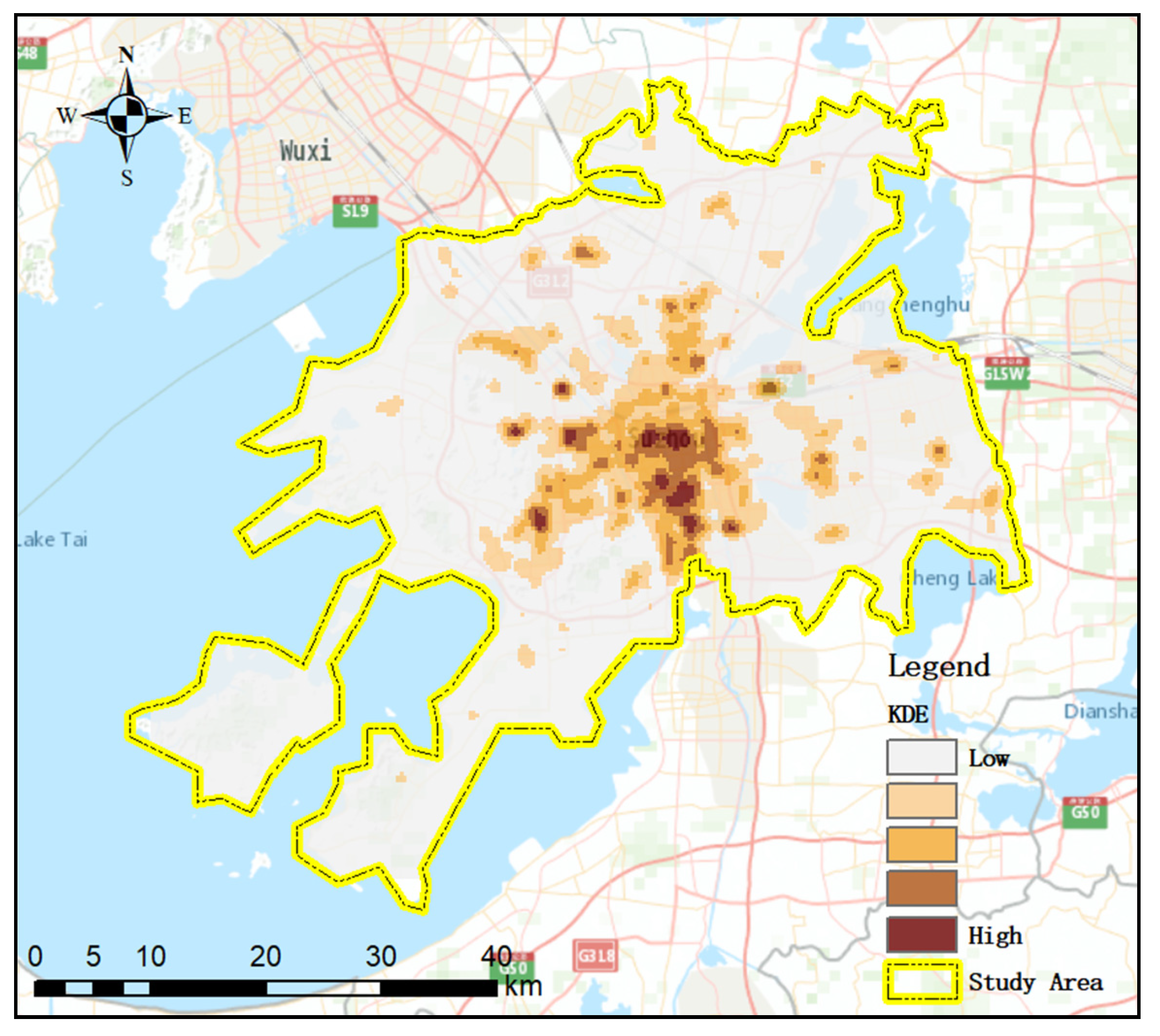
Suzhou City, with a population of approximately 10,616,000 people, is located in southeastern Jiangsu Province, China. It is the city with the sixth-highest GDP in China. The Yangtze River is to the north of Suzhou and Taihu Lake (the third-largest freshwater lake in China) is to the west of Suzhou. Suzhou is an important city of the Yangtze River Delta urban agglomeration in the Taihu Lake Basin, where the economy is active and transportation is widely available. A solution for effective crime prediction that can be applied to each area is necessary to help the police arrange their force and reduce the crime rate. Among the five municipal districts of Suzhou, we selected the four that account for more than 80% of the city’s criminal cases from 2012 to 2013, namely, Huqiu District, Gusu District, Wuzhong District, and Xiangcheng District, and eliminated their water areas to create our study area.
Figure 1 shows the kernel density estimation of all property crimes (over 130,000 cases) in the study area from January 2012 to October 2013. The crime data were acquired from the local police department, and the dataset contains the case number, crime type, occurring time, geographical coordinates, etc. In this paper, our target crime types were burglary, theft, and robbery, which are classified by the police as common types of property crime in Suzhou [3,49,50].
2.2. Weather Data
Weather can influence crime rates and criminal behavior, and each variable has a diverse effect on different crime types [51,52,53]. In short-term crime prediction, weather variables are common predictors, and temperature is a significant one for property crime prediction [29,54]. In this study, we chose temperature as the external influence of the model. Data on daily average temperature, highest temperature, and lowest temperature data for the 671 days from January 2012 to October 2013 were collected from the China Ministry of Agriculture Planning and Design Institute [55].
3. Methodology
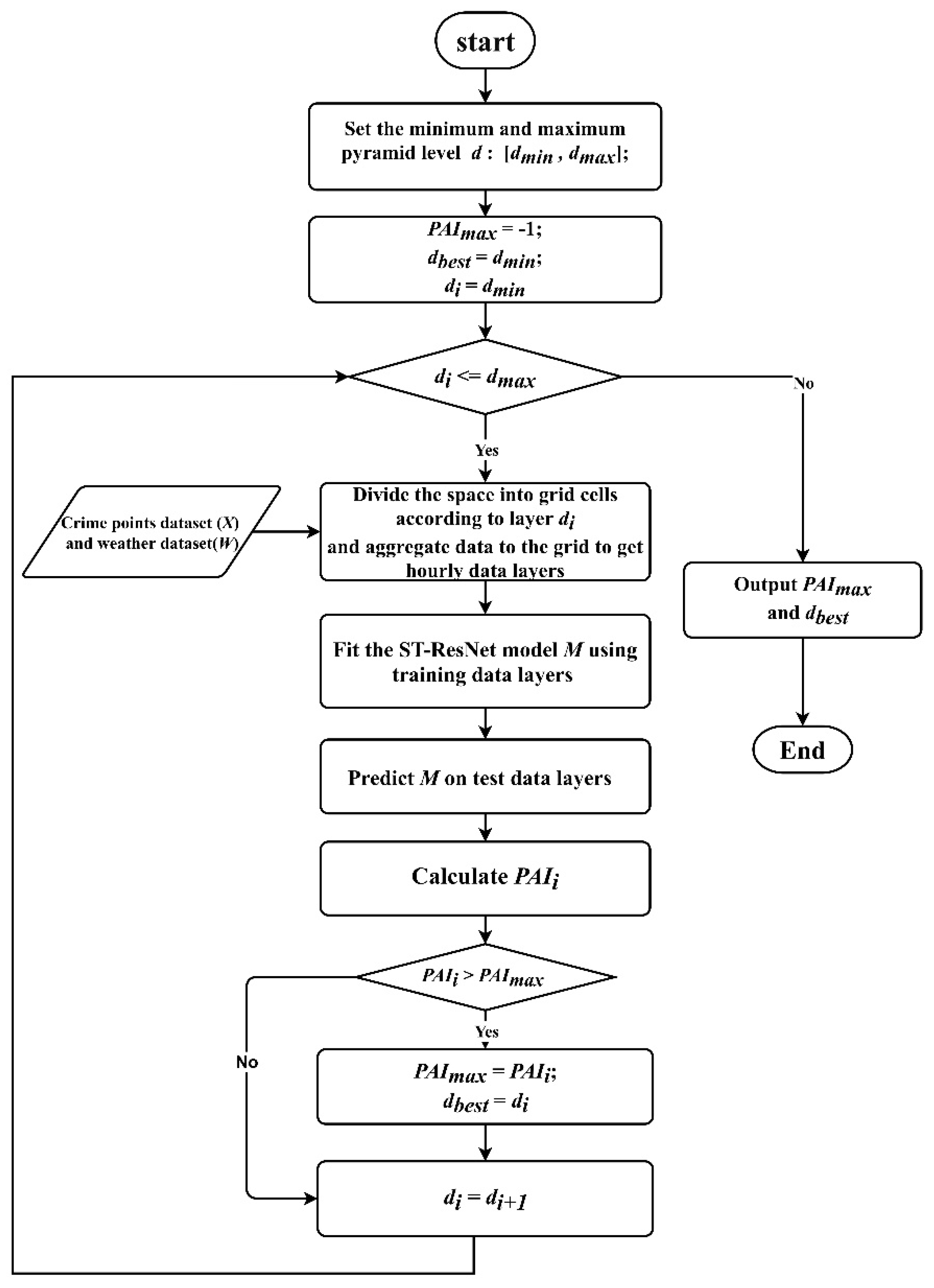
To improve the effectiveness of hourly crime prediction, we proposed an adaptive spatial resolution method to select the optimal unit for crime prediction models. The ST-ResNet model was used to predict the crime risk. The PAI was used to measure the accuracy of the results at different spatial resolutions [29]. Figure 2 indicates the procedure of the method.
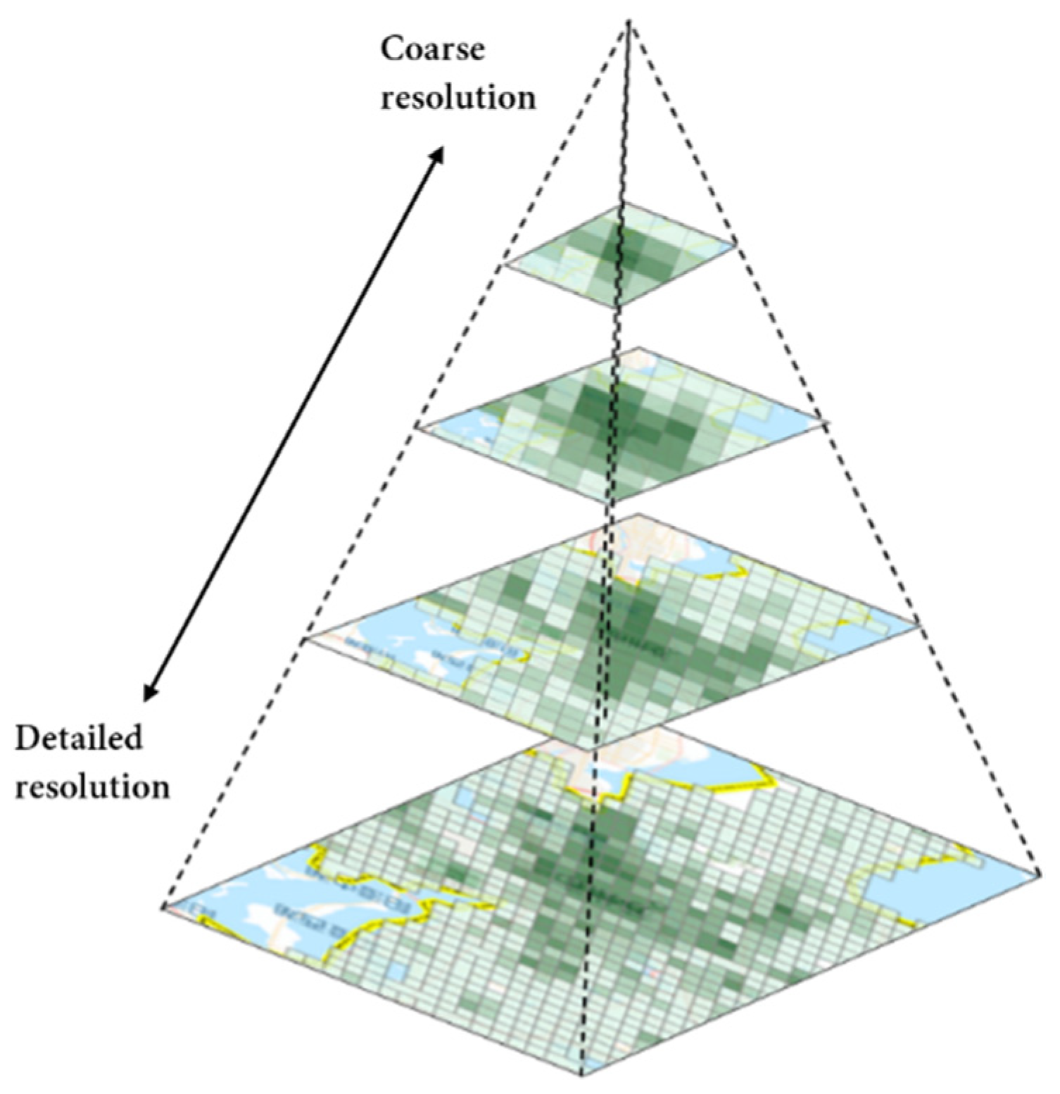
A data pyramid [56] was produced to aggregated points to the grid at multiple scales, as shown in Figure 3. Most web mapping services like Google Maps and Microsoft Bing Maps adopt the pyramid technique to provide on-demand map content to users [57,58]. The discretization method we used is the same as in these web mapping services. The procedure starts with a coarse resolution and then recursively generates the other resolutions. The points are aggregated to the layers in each calculation of the ST-ResNet model. The base resolution is set to 9.6 km, which corresponds to the 12th level of the pyramid according to the local maximum patrol area.
The research area was overlaid by grid cells of various resolutions. The high-resolution layer has small grids that cover a small area and the low-resolution layer has large grids that cover a large area. The crimes were aggregated to the space time grids based on their geocoordinates and time. The number of crimes was counted by grid and assigned to the corresponding cells of a layer.
For the weather data, the grid cells of a time layer share the same value because the weather is homogeneous over the research area. The established layers were divided into training data and test data. Training data were used to train the ST-ResNet model M (as discussed in Section 3.1) and identify the optimal parameters in a certain spatial resolution. Then, the crime risk was calculated with test data evaluated by the PAI.
By increasing the level of layer d in the pyramid, the resolution of the grid is increased. The crimes were re-aggregated to the grids of another layer. To minimize the influence of time variation of crime, crimes committed over 12 months were selected as training data and the crimes committed in the following month were selected to verify the accuracy of the model. This process was carried out recursively for certain times until the highest-resolution layer was obtained. PAI was included in the model to evaluate the accuracy of the calculations.
3.1. ST-ResNet Model
The ST-ResNet model predicts crime risk based on weather records as well as crime patterns including trend, period, and closeness (Figure 4). The trend indicates the tendency of the number of crimes to increase or decrease. The period refers to the periodic pattern of crime at a certain time scale. Compared with distant ones, crimes committed closer together in time are more likely to be related. Therefore, “closeness” refers to the time distance between crime pairs. Following the research of Wang (2019), the experiment adopted hourly, daily, and weekly levels as the time spacings of the 3 crime periodic characteristics [29].
Figure 4 shows the process of the ST-ResNet model. In the convolution step, multilayer convolution is selected to measure the relationship between nonadjacent regions. The 3 periodic components and the external component (weather) are fused via a parametric-matrix-based fusion method.
The model utilizes the historical crime spatial distributions and weather records to predict crime spatial distribution at time , where , ,…, are the layers representing crime spatial distributions at times , ,…, and , ,…, are the weather layers.
We minimized the root-mean-square error (RMSE) between the predicted crime matrix and the true crime matrix to train the model:
where is the true value, is the predicted value, and Z is the number of training data points [59].
The modeling process was conducted as follows: A training dataset (from January 2012 to December 2012) was used to train the model with cross-validation (20% validation ratio), and a test set (from January 2013 to October 2013) was used to test the final model. The model was trained over multiple iterations to select the final model, with the optimal tuning parameters based on minimizing the cross-validation error. Then, we made predictions about the test set using the final model and evaluated the prediction effect. Accounting for the fact that seasonal differences potentially influence results, for each month of the test set we repeatedly predicted crime events for each variation of the methodological parameters. That is, for each variation, predictions were made using a rolling window (e.g., when predicting for January 2013 using 1 year of historical data, the data from January 2012 to December 2012 were used for training; when predicting for February 2013, data from February 2012 to January 2013 were used; and so on): the prediction accuracy was calculated for each month and then averaged for each variation for the test set.
3.2. Accuracy Evaluation
The RMSE, which evaluates the difference between the predicted and the values observed, and the F1 score [60], which evaluates the precision and recall, are scale-dependent. A commonly used crime prediction evaluation index is the prediction accuracy index (PAI) [6]. This can be used to compare the accuracy of hotspots calculated by different methods via extremely simple calculations and can compare the prediction results at different resolutions and magnitudes. The general form of this variable is as follows:
where is the number of crime events in areas where crimes are predicted to occur. is the number of actual crime events in the whole study area. is the area of regions where crimes are predicted to occur. is the area of the study area. The PAI can be considered as the hit rate in areas where crimes are predicted to occur with respect to the size of the study area. The higher the hit rate and the better the prediction effect, the higher the PAI will be.
4. Results
4.1. Data Analysis
Crime risk measured by a repeat and near-repeat calculator varies among different crime types [52]. We calculated the proximity, periodicity, and heterogeneity of crimes in space and time. Finally, the correlation between temperature variation and crime level was tested.
Figure 5 shows the daily statistics, 7-day moving average data, 14-day moving average data, and 30-day moving average data for property crime events from January 2012 to October 2013.
The near-repeat calculator uses the Knox test to analyze the coordinates within a given time span by Monte Carlo simulations to detect the near-repeat phenomenon [61]. We set a spatial bandwidth of 300 m because the block length of our study area is about 300 m. We set the temporal bandwidth at 7 days. The Manhattan distance was used because it is close to an approximation of the actual route for urban environments. Table 1 shows the crime risk level in a near-repeat matrix; in the case of our study area, there was a significant near-repeat pattern for the first week within 300 m, and the near-repeat phenomenon weakened with time and distance.
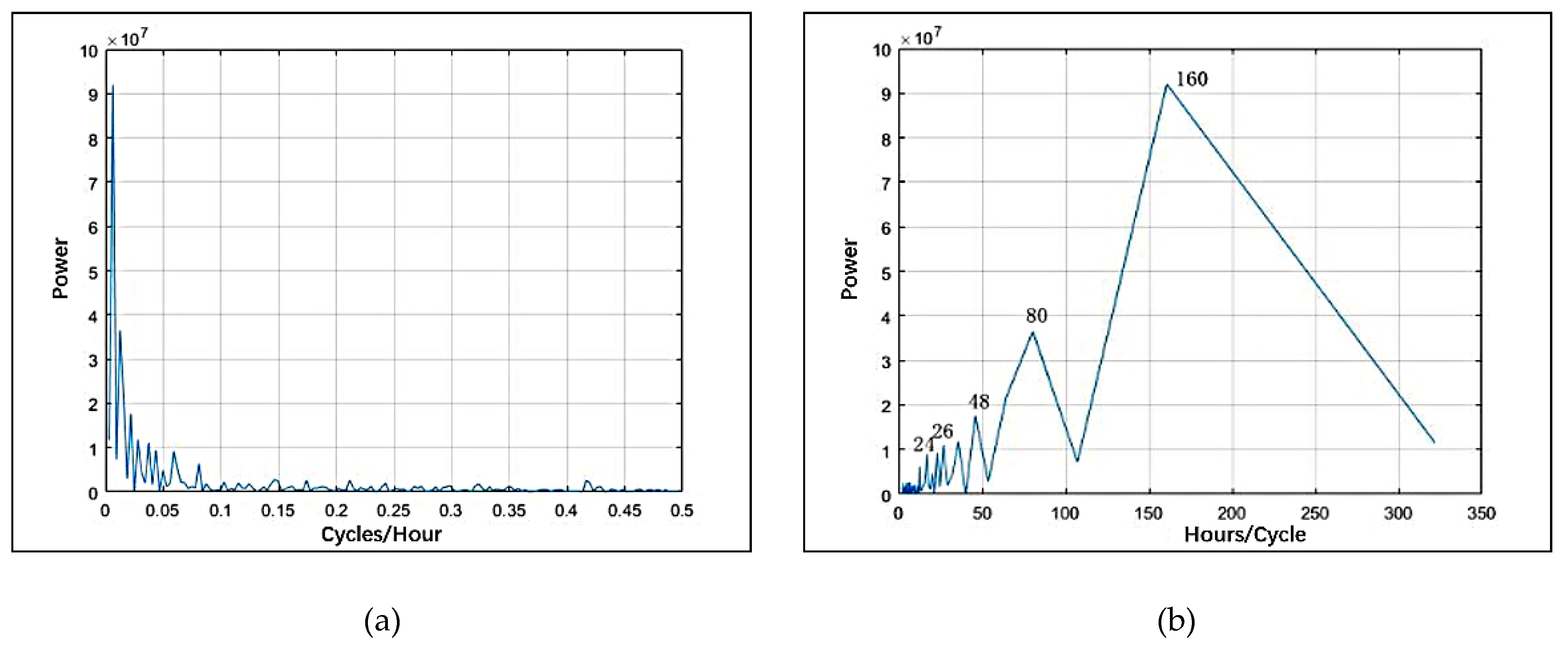
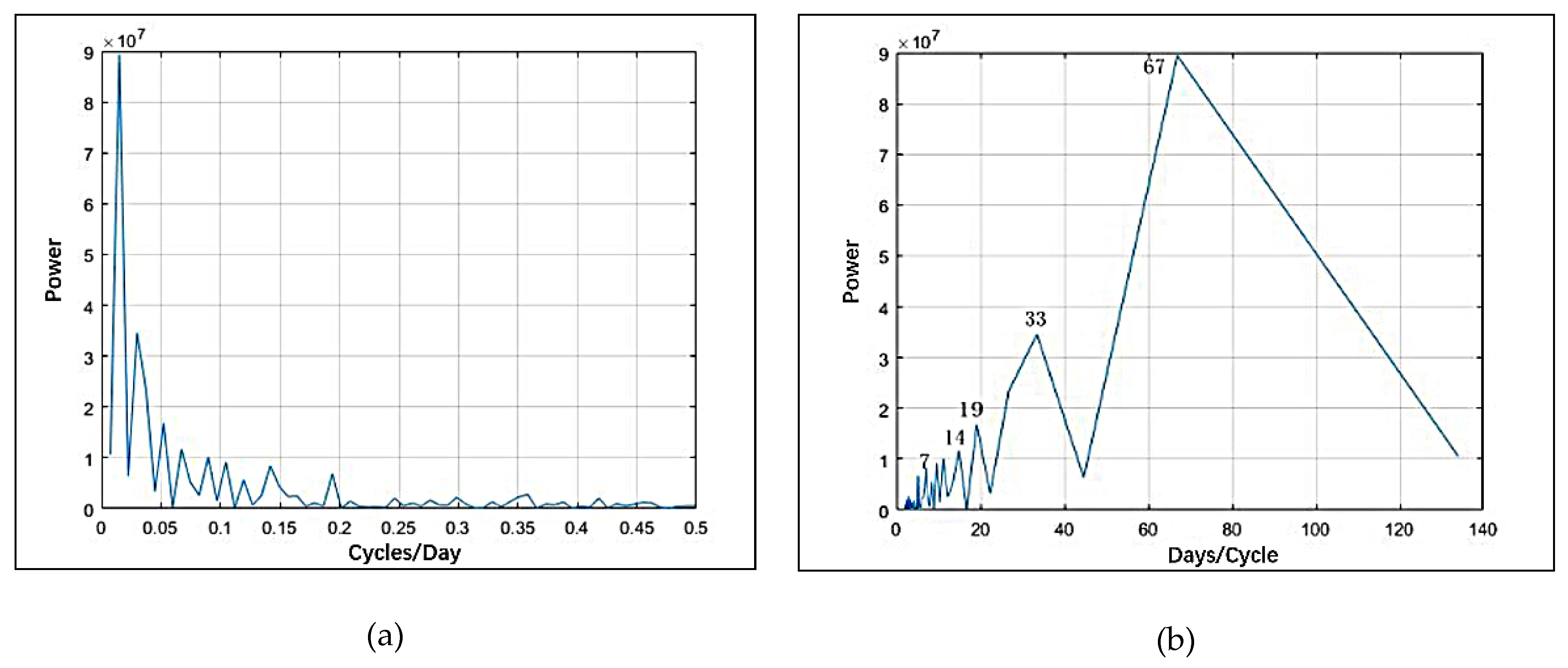
The power spectrum method [62] is used to calculate the periods of crime data. The magnitude squared of Fourier coefficients is a measure of power. The power is computed on one-half of the coefficients since half of them are repeated in magnitude. We plotted the power spectra as a function of frequency, measured in cycles per hour and per day. To interpret the view of the cyclical activity more easily, we also plotted power as a function of period, measured in hours and days per cycle. Figure 6 shows the power spectrum (a) and the period of the hourly data (b). The average periods passing the significance test are 24 h, 48 h, 80 h, and 160 h. The repeating short-term cycle can be seen in daily periodicity. Figure 7 shows the power spectrum (a) and the period of the daily data (b). The average periods passing the significance test are 7 days, 14 days, 19 days, 33 days, and 67 days. This shows the weekly trend of the crime data.
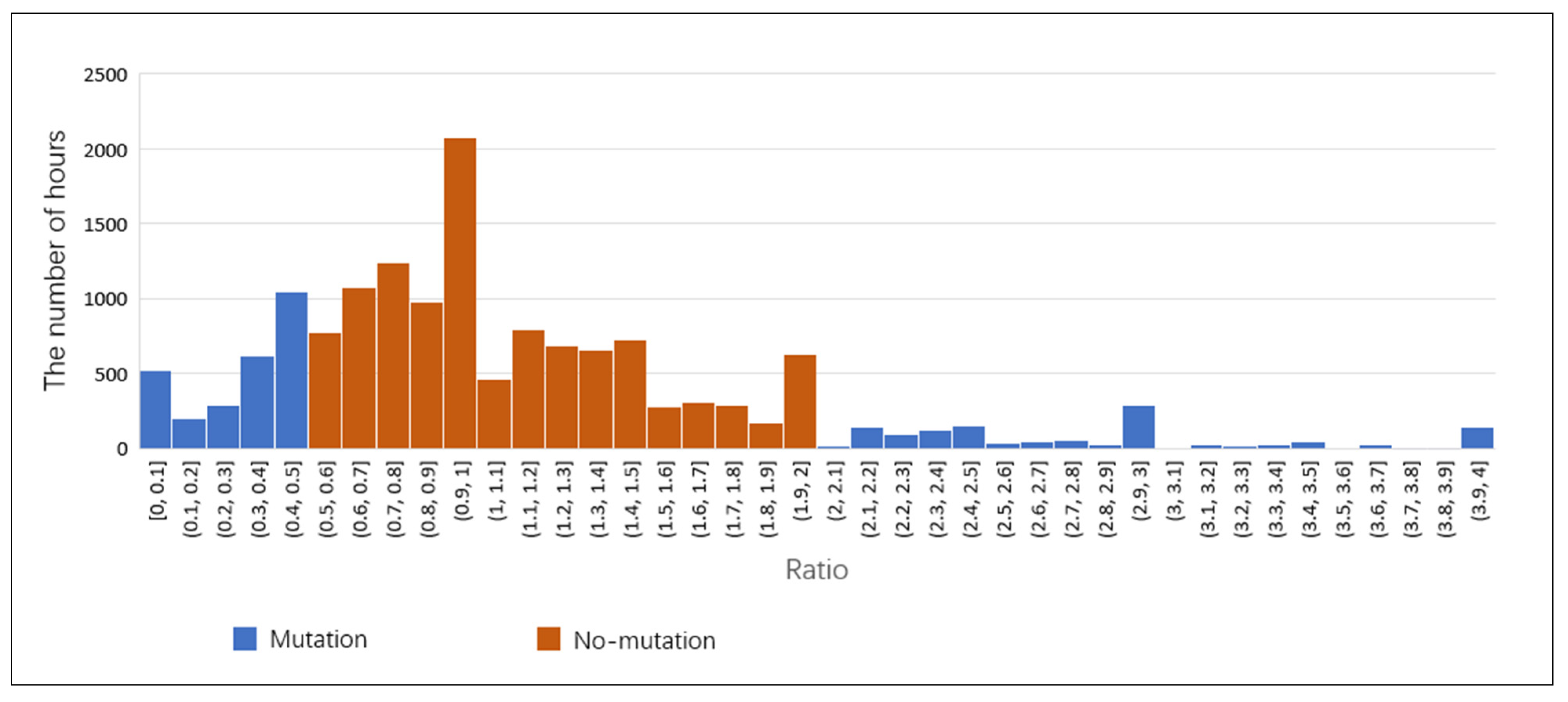
We calculated the ratio of the number of cases in adjacent hours, excluding some moments with abnormally high or no cases; then, we counted the number of hours corresponding to each ratio value from January 2012 to October 2013. Figure 8 shows the ratio statistics. Ninety-five percent of adjacent hours have a ratio of cases between 0 and 4. Considering that the number of cases per hour is small, we defined the times when the ratio value was between 0.5 and 2 (which means the change rate is no more than 100%) as no-mutation hours and the times when the ratio value was less than 0.5 or greater than 2 as mutation hours. We also calculated the ratio of the number of cases between periods of two-hour intervals and three-hour intervals. Table 2 shows the percentages of no-mutation hours in the three situations. Although the percentage of no-mutation hours decreased as the time interval increased, it was still high for all three intervals. Therefore, it can be concluded that there are interactions between the cases at adjacent moments (1–3 h).
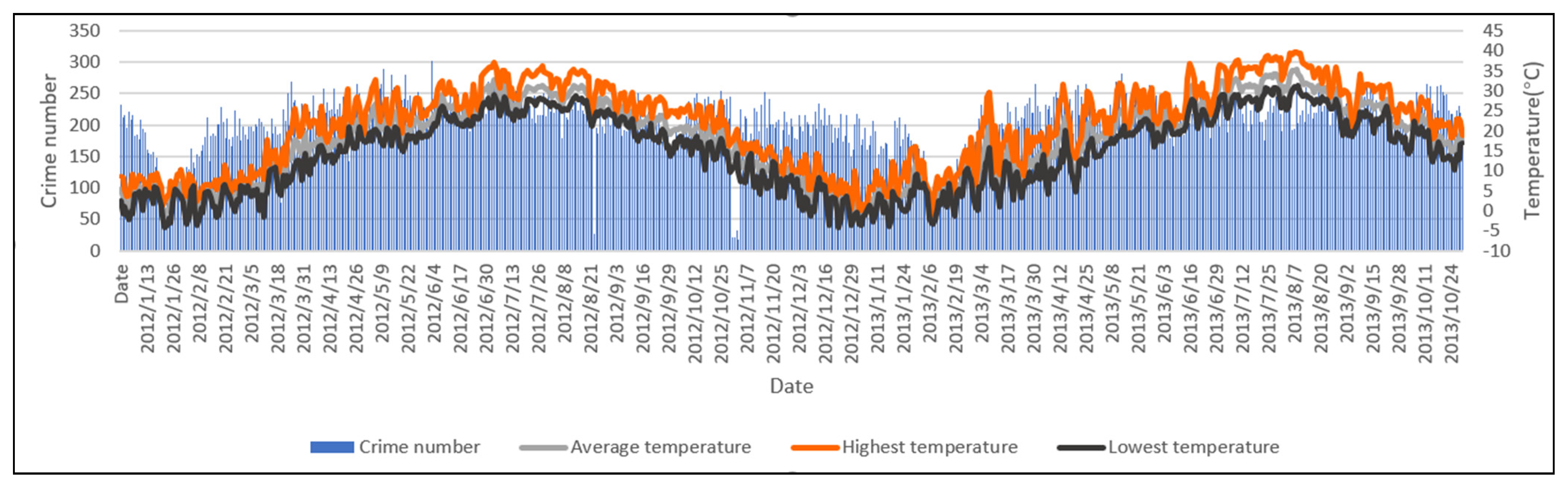
Figure 9 shows the changes in daily temperature variables and crime number, and their trends possess a certain relevance. Considering that the study area is a part of a city, there is no significant spatial variation of temperature in this area. Thus, we only analyzed the impact of temperature on crime data over time. A Pearson correlation analysis [63] was used to examine the relationships between the daily temperature variables and crime number. Table 3 shows the results. The daily temperature variables (average temperature, highest temperature, and lowest temperature) are significantly highly correlative. We chose the daily highest temperature, which is most relevant to the crime number, to use in the crime number regression analysis [52]. The result (R2 = 30.9%) indicated that the highest temperature can explain 30.9% of the variance in property crime.
4.2. Data Aggregation
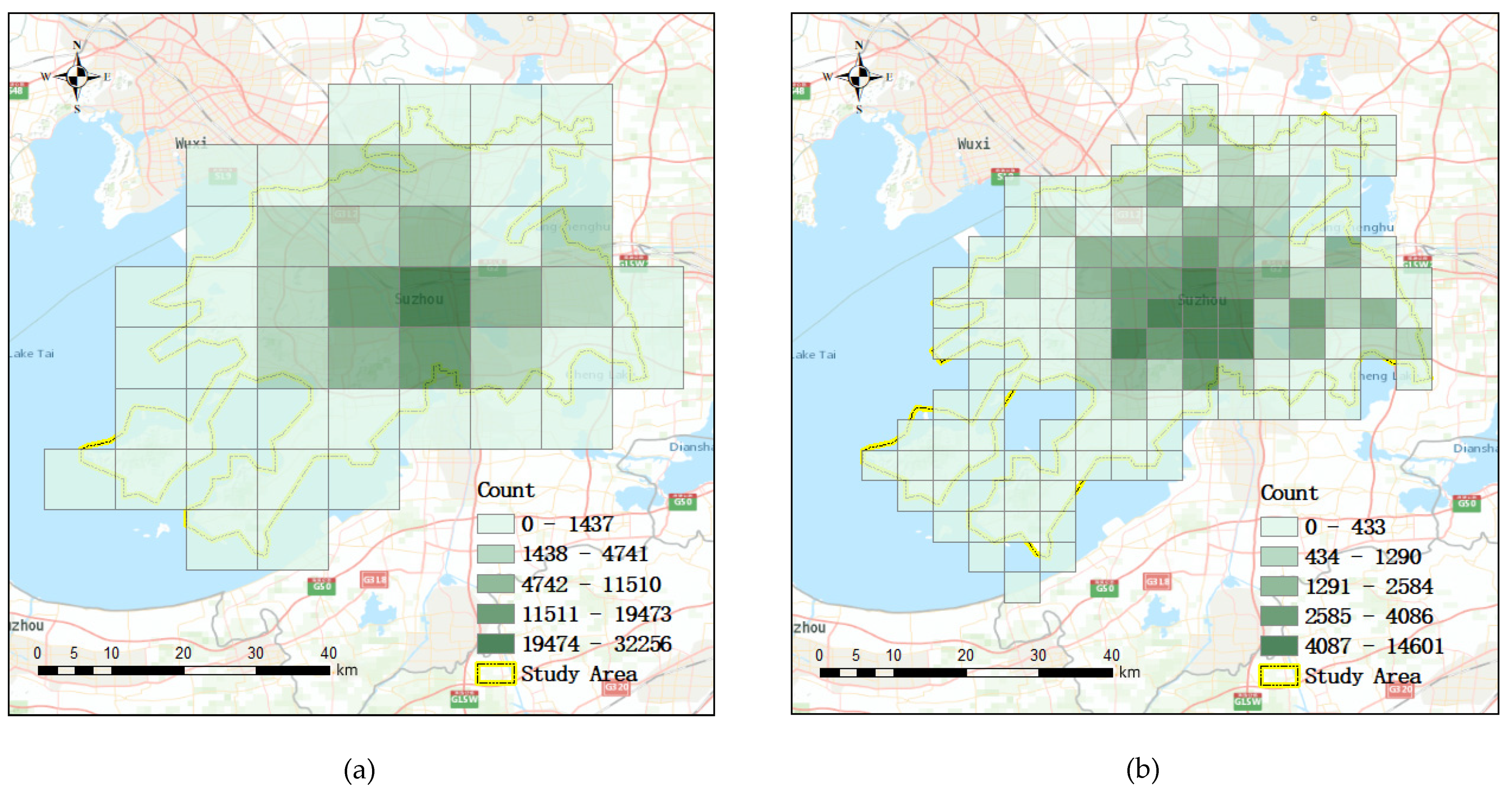
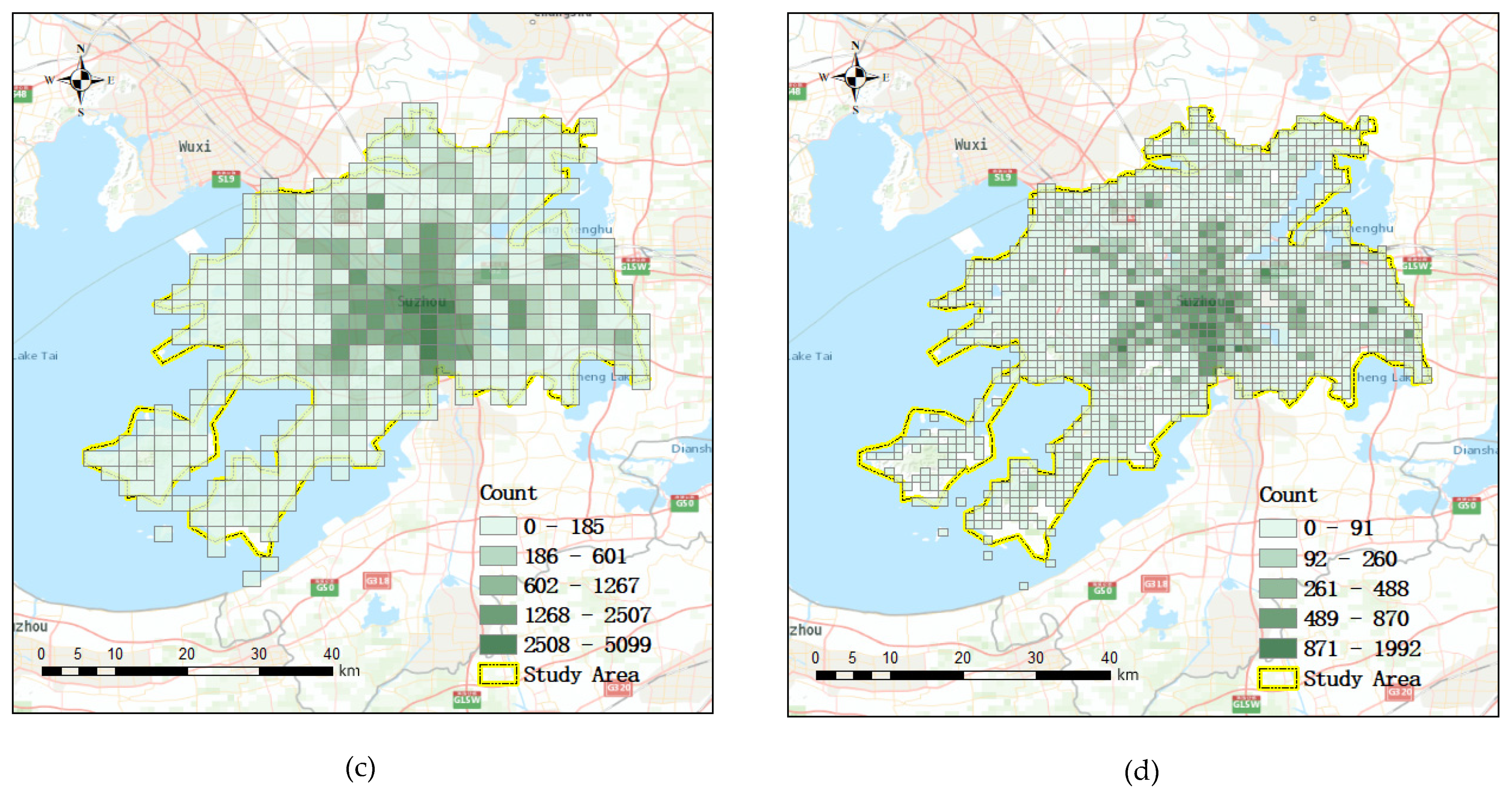
Figure 10 shows the property crime distribution at different spatial resolutions from January 2012 to October 2013. The information of different spatial resolutions of the study area is shown in Table 4. There is a strong clustering characteristic for the crime distribution. The cases are mainly concentrated in the center of the study area.
4.3. ST-ResNet Model for Crime Prediction in Suzhou
We divided the training data from 2012 between a training set and a validation set at a proportion of 9:1. RMSE was employed as the evaluation metric to tune the main hyperparameters to identify the optimal parameters for ST-ResNet models at each resolution, including convolution kernel size, number of convolution kernels, network depth, and length of closeness, period, and trend. The early stopping strategy was adopted to prevent overfitting [64,65]. The training procedure stopped when the RMSE of the validation set was not attenuated for 5 iterations.
We compared the RMSEs between predictions and validation data with different parameters at each resolution. The optimal ST-ResNet model should be constructed with a 3 × 3 convolution kernel size (Appendix A Table A1), 64 convolution kernels (Appendix A Table A2), 8 residual network units (Appendix A Figure A1), and the 3 temporal components (1 h, 1 day, and 1 week) (Appendix A Figure A2, Appendix A Figure A3, Appendix A Figure A4, respectively). According to the previous analysis, the highest daily temperature is proven to be a significant external factor affecting property crimes. In this model, we selected highest daily temperature as the external component.
4.4. Selection of the Optimal Spatial Resolution
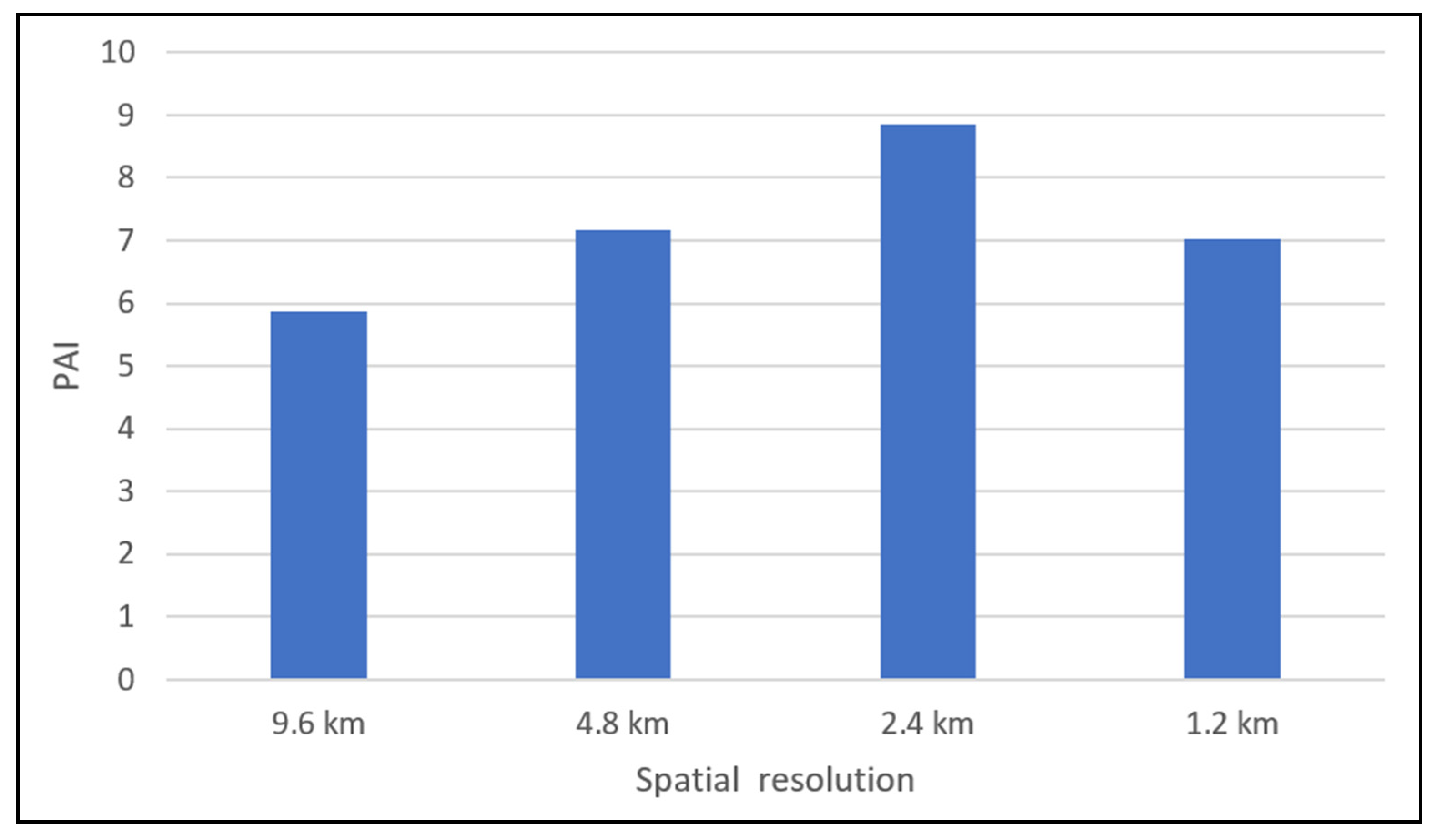
We ran models with optimal hyperparameters at different spatial resolutions (from 1.2 km to 9.6 km) and calculated the PAI of the prediction results (shown in Figure 11). The highest PAI was achieved with a 2.4 km spatial resolution in our study area with RMSE = 7.81.
4.5. Evaluation of the Prediction Results
Based on the previous results, the optimal ST-ResNet model is conducted with a 2.4 km spatial resolution. With the test dataset, we calculated its average evaluation indicator values for its prediction results for PAI = 8.8.
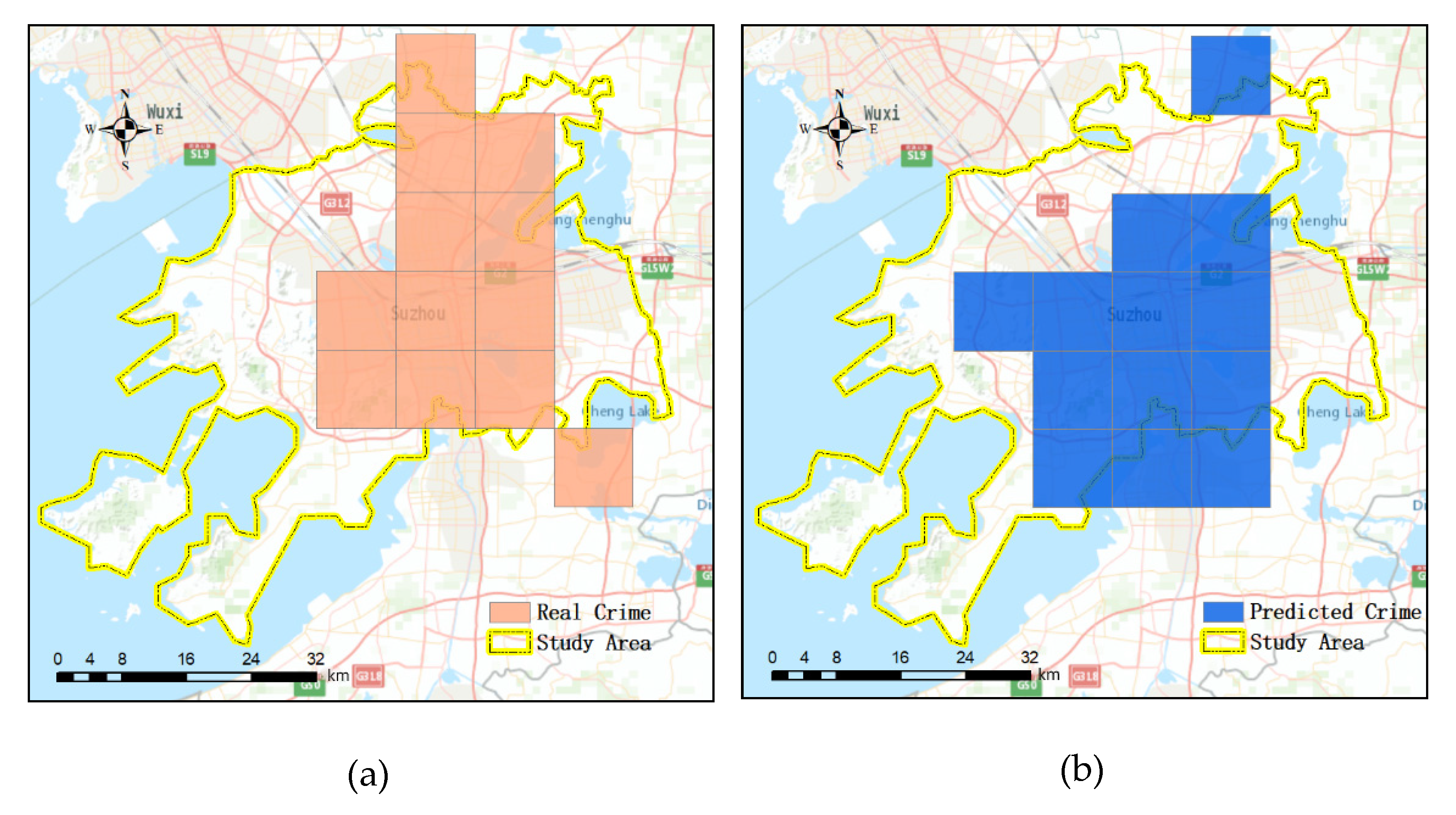
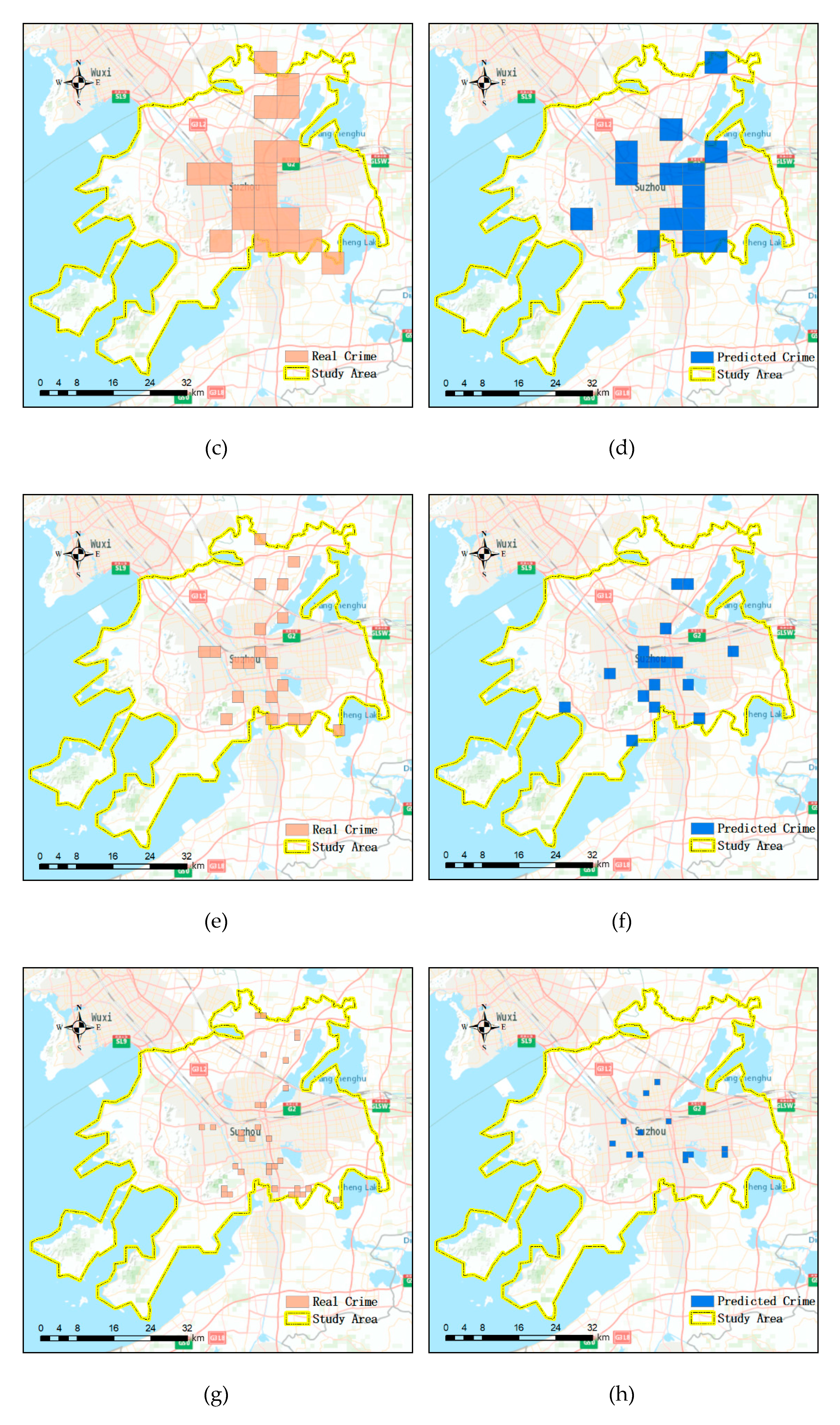
Figure 12 shows the prediction results and the actual distributions at the different four resolutions at 12 a.m. on 1 January 2013. Binary maps were adapted because the crime prediction evaluation index PAI deals with a place being a crime hotspot or not (binary). Colored grids represent the occurrence of crimes. In general, true prediction results are concentrated in city centers, which are areas with high crime densities; in edge areas, predictions are poor. Although the similarity between the prediction results and the actual distributions decreases with increasing resolution, there is a trade-off between the grid size and practical police force arrangement. PAI values of prediction results at a 1.2 km resolution (Figure 12b), 2.4 km resolution (Figure 12d), 4.8 km resolution (Figure 12f), and 9.6 km resolution (Figure 12h) resolution are 2.7, 5.9, 9.8, and 3.3, respectively. Larger grid cells can capture more criminal activities but lead to difficulties for police arrangements. Finding crime hotspots with an appropriate grid cell size is crucial to arranging police forces effectively.
5. Conclusions and Future Work
We proposed an adaptive spatial resolution method to select the best spatial resolution for crime prediction at hourly temporal scales based on the ST-ResNet model. In this paper, we discussed the property crime distribution characteristics and the corresponding weather impact factors. Interactive relationships between crimes close in time were confirmed. The periodic characteristic of crime in days and weeks was tested. Spatially, crimes are often clustered, and the degrees of regional crime event clustering at different spatial resolutions are distinct. A pyramid layering model was built to perform the information of different resolutions. The method we proposed can improve the accuracy of the hourly crime prediction model adopted in the research of Wang (2019) by selecting an optimal resolution for it [29]. We believe the current results can be used to allocate police resources more efficiently.
In this study, the results showed that the optimal unit of analysis was neither the finest nor the broadest considered, but an intermediate unit. This is consistent with the research of Ramos et al. (2020) and Malleson et al. (2019) [44,45]. Ramos et al. (2020) recommended crime maps with intermediate granularity as being the most reliable, because coarse granularities may mask crime hotspots and too-fine granularities may make crime counts unstable and unrepresentative [45]. Similarly, Malleson et al. (2019) recommended medium-granularity maps for point data aggregation because they can balance the benefits of smaller units (important heterogeneity which will probably be hidden in larger units is apparent when using smaller units) and the drawbacks of larger ones (including unstable and unrepresentative crime counts) [44].
By contrast, some researchers concluded that “smaller is better” in granularity choice for crime analysis [39,43]. These studies focus on the impact of the social environment on crime level from a micro view. A micro-view analysis may provide the relationship between crime level and its impact factors in small areas. However, these results cannot be used for police deployment. Our method is used to find the most appropriate unit for improving the hit rate of the predicted crime hotspots. The result is expected to improve the local police deployment and deter crime.
Many factors can affect criminal behaviors, and their impact varies in different situations. The occurrence of crime is usually the result of multiple factors. This paper only discusses the temperature factor, and the auxiliary explanation is insufficient. More factors will be considered in future work. Their impact on crime will be analyzed and combined to improve the interpretation of crime to improve the prediction accuracy.
Author Contributions
Conceptualization, Hong Zhang and Zengli Wang; Data curation, Hao Yin; Formal analysis, Hao Yin; Funding acquisition, Hong Zhang; Investigation, Jie Zhang and Hao Yin; Methodology, Hong Zhang, Jie Zhang, and Hao Yin; Project administration, Hong Zhang; Resources, Hong Zhang; Supervision, Hong Zhang; Validation, Jie Zhang; Visualization, Jie Zhang; Writing—original draft, Jie Zhang; Writing—review and editing, Zengli Wang. All authors have read and agreed to the published version of the manuscript.
Funding
This research was funded by the National Key Research and Development Program (grant numbers: 2018YFB0505500, 2018YFB0505504) and the National Natural Science Foundation of China, (grant number: 41471372).
Institutional Review Board Statement
Not applicable.
Informed Consent Statement
Not applicable.
Data Availability Statement
Data available on request due to privacy restrictions.
Acknowledgments
We thank the anonymous reviewers and academic editor for the constructive suggestions and insightful comments which substantially improved the quality of this research.
Conflicts of Interest
The authors declare no conflict of interest.
Appendix A
Table A1 lists the RMSEs between predictions and validation data at different spatial resolutions with different convolution kernel sizes. The same hyperparameters were used: number of convolution kernels = 16, network depth = 4, length of closeness = 1 h, length of period = 1 day, length of trend = 1 week. The results showed that 3 × 3 is the optimal convolution kernel size for the model. A larger kernel will cover a larger spatial region, but for the same receptive field, the stacking of small multilayer kernels is beneficial to detect more complex nonlinear features than a single-layer larger kernel [66].
Table A2 lists the RMSEs between predictions and validation data at different spatial resolutions with different numbers of convolution kernels. The other parameters remain the same. The number of convolution kernels varies between 16, 32, 64, and 128. The RMSEs initially decrease with the increase in numbers of convolution kernels and reach their minimum values when the number is 64. Although a large number of convolution kernels can be used to accurately extract the distribution of features, too many convolution kernels can lead to overfitting problems. The optimal number of convolution kernels for the model is 64.
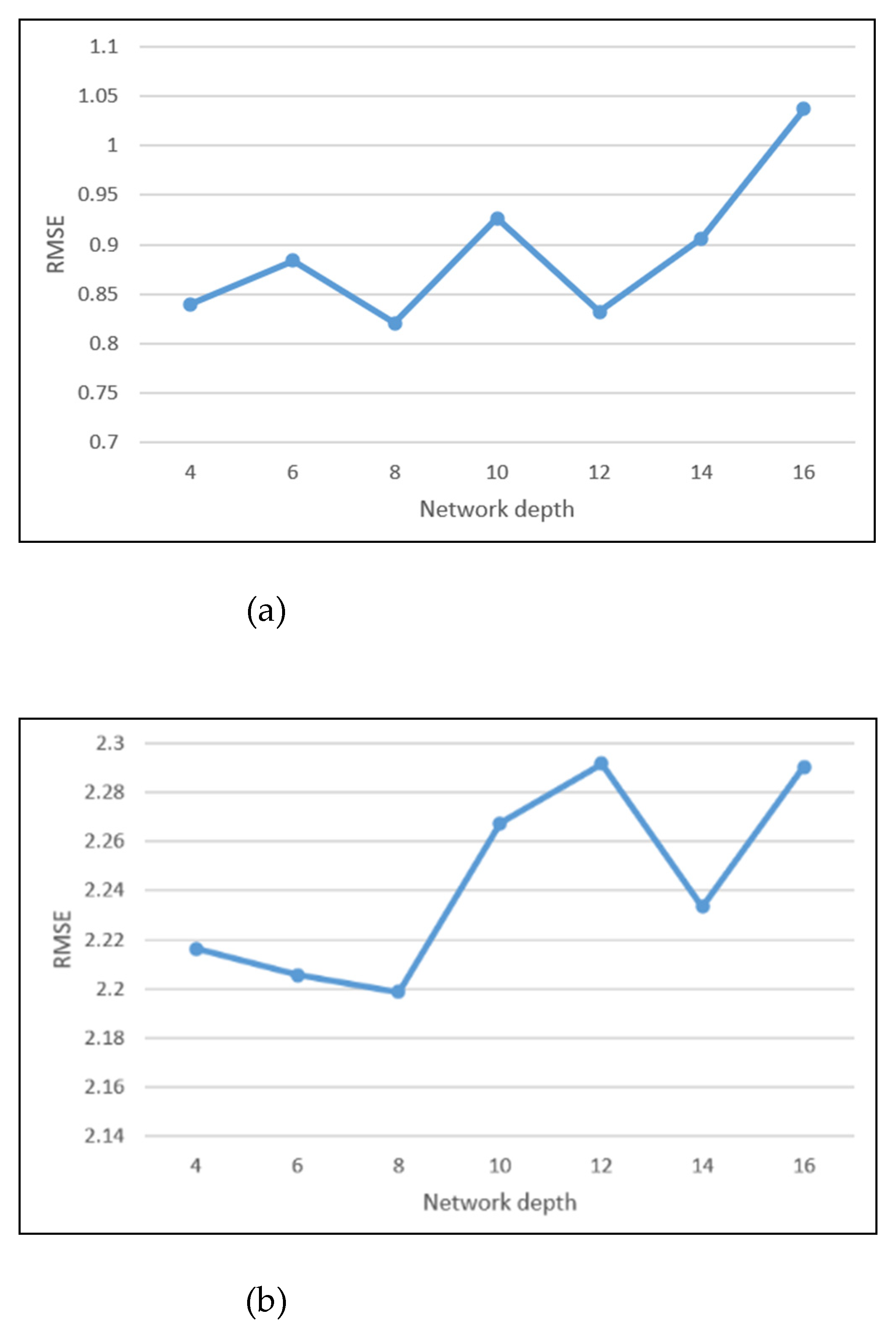
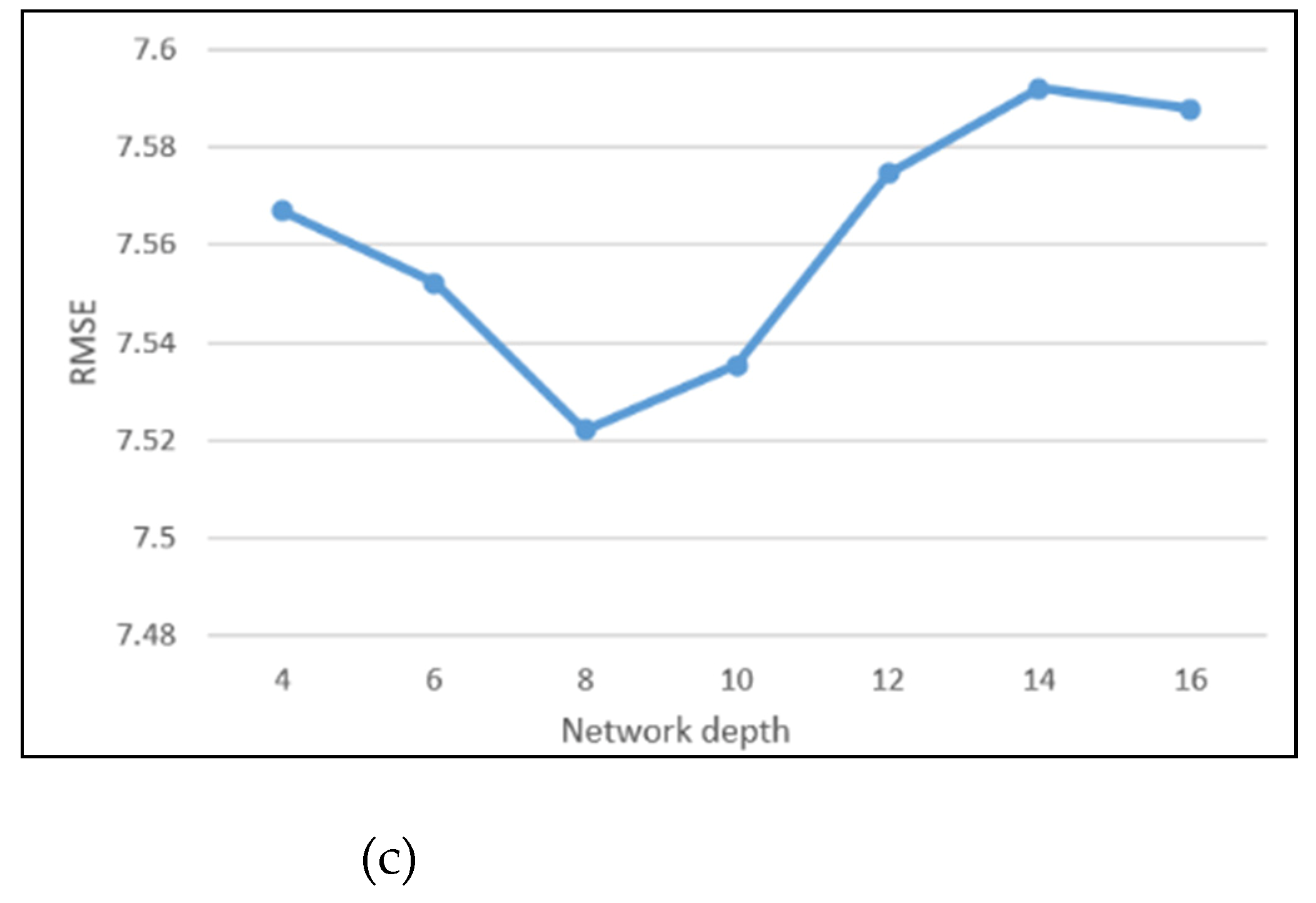
Figure A1 shows the influence of the network depth on the training results at different spatial resolutions. The residual network unit represents the network depth. The depths vary from 4 to 16 in step two. As the network goes deeper, the RMSEs initially decrease and reach their minimum values when the depth is eight. Subsequently, the RMSEs increase. Training difficulty and noise at the city fringe will be introduced with the addition of layers. Thus, the optimal network depth for the model is 8 ResNet units.
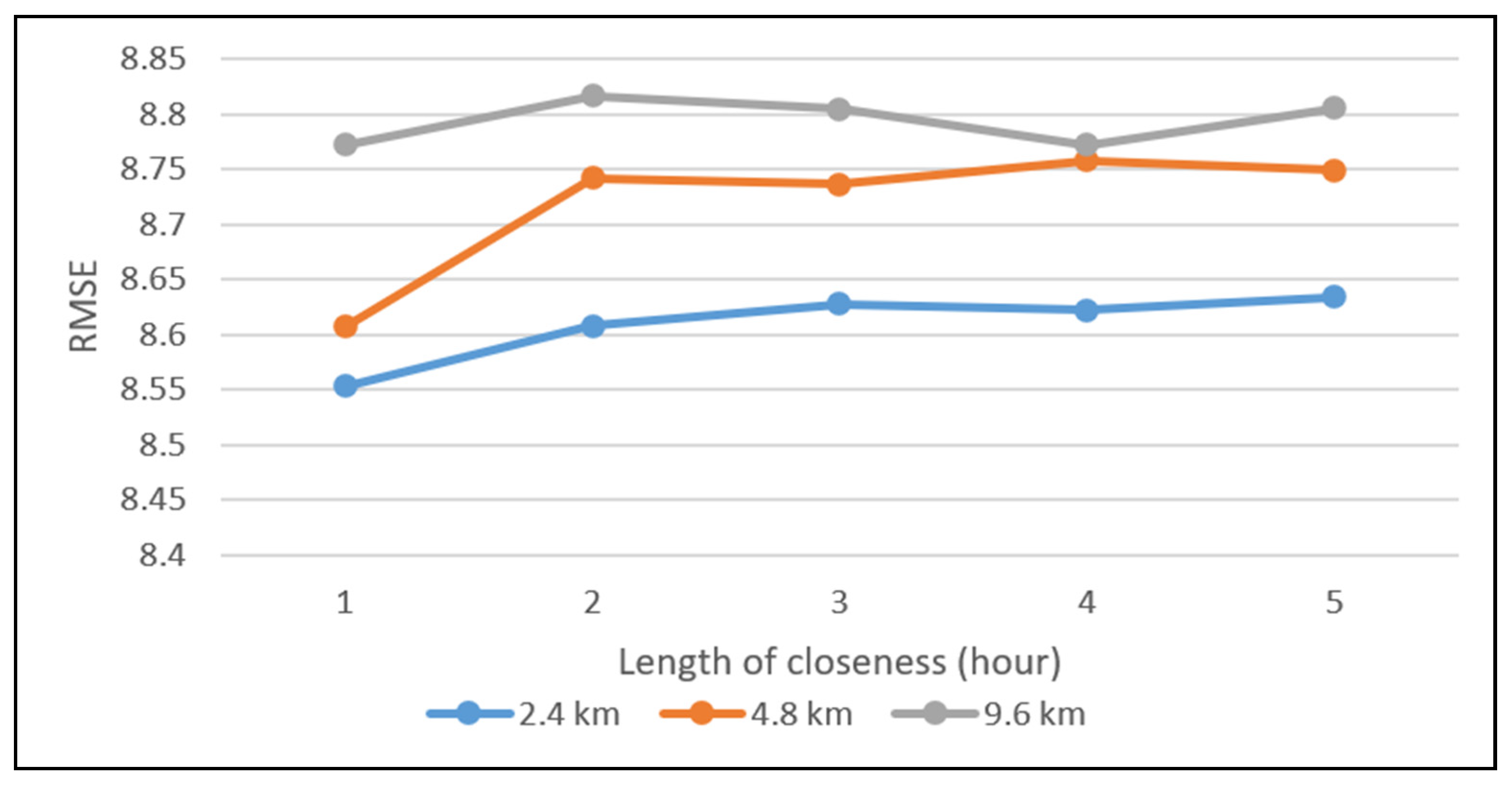
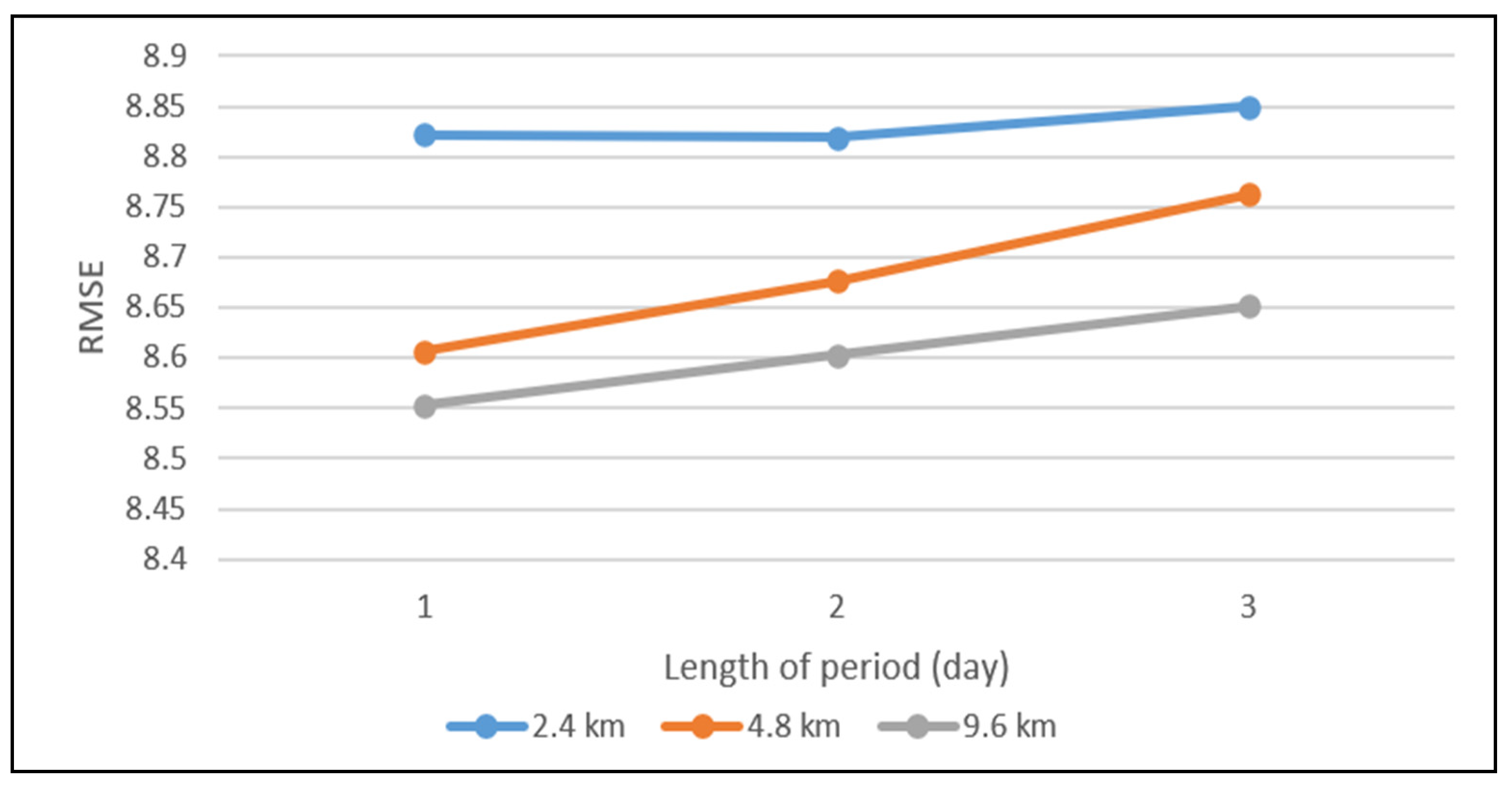
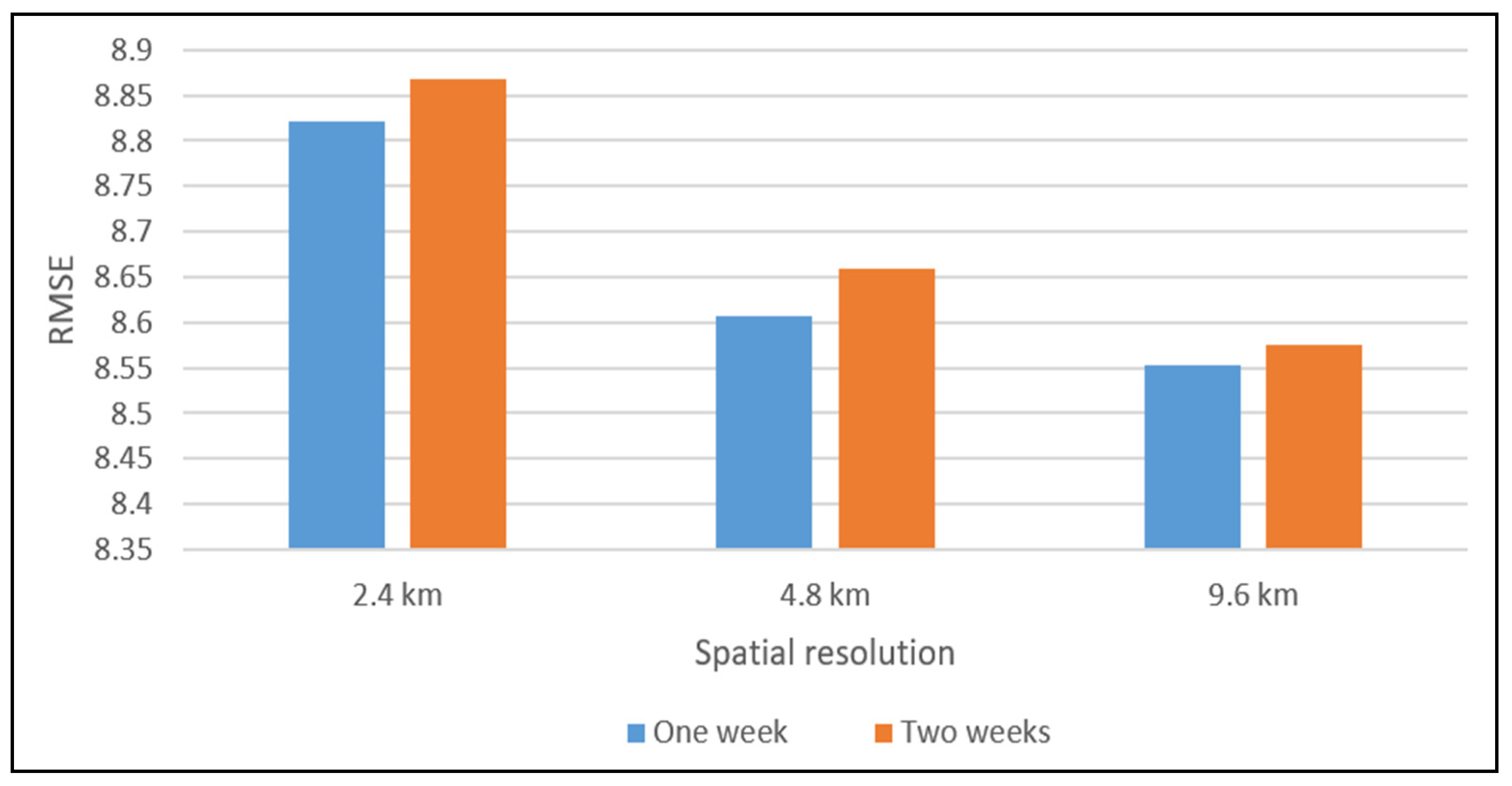
The impacts of temporal components, including closeness, period, and trend at different spatial resolutions, are also verified. Figure A2 shows the variations in RMSEs at different spatial resolutions with different lengths of closeness, where we fix the length of period to 1 day and the length of the trend to 1 week. The RMSEs are minimal when the length of closeness is 1 h. Compared with distant hours, crimes between two adjacent hours are more relevant. Figure A3 shows the variations in RMSEs at different spatial resolutions with different lengths of period where we fix the length of closeness to 1 h and the length of the trend to 1 week. We can observe that RMSEs decrease as the length of the period increases. A period length of 1 day leads to the best RMSEs, indicating that short-range periods tend to be beneficial, while long-range periods may be difficult to model. Figure A4 shows the variations in RMSEs at different spatial resolutions with different lengths of trend, where we fix the length of closeness to 1 h and the length of period to 1 day. We can see that a trend length of 1 week leads to the best performance. Similar to periods, long-range trends may be more difficult to capture.

Table A1.
RMSEs at different spatial resolutions with different convolution kernel sizes.
| 3 × 3 | 5 × 5 | 7 × 7 | |
|---|---|---|---|
| 2.4 km | 8.553 | 8.590 | 9.047 |
| 4.8 km | 8.607 | 10.807 | 10.819 |
| 9.6 km | 11.422 | 11.504 | 78.614 |
Table A2.
RMSEs at different spatial resolutions with different numbers of convolution kernels.
| 16 | 32 | 64 | 128 | |
|---|---|---|---|---|
| 2.4 km | 8.670 | 8.639 | 8.553 | 8.604 |
| 4.8 km | 8.883 | 8.760 | 8.607 | 8.659 |
| 9.6 km | 11.386 | 11.258 | 11.222 | 11.331 |
Figure A1.
RMSEs for different spatial resolutions and network depths: (a) RMSEs for different network depths at a 9.6 km spatial resolution; (b) RMSEs for different network depths at a 4.8 km spatial resolution; (c) RMSEs for different network depths at a 2.4 km spatial resolution.
Figure A1.
RMSEs for different spatial resolutions and network depths: (a) RMSEs for different network depths at a 9.6 km spatial resolution; (b) RMSEs for different network depths at a 4.8 km spatial resolution; (c) RMSEs for different network depths at a 2.4 km spatial resolution.


Figure A2.
RMSEs at different spatial resolutions with different lengths of closeness.

Figure A3.
RMSEs at different spatial resolutions with different lengths of time.

Figure A4.
RMSEs at different spatial resolutions with different lengths of trend.

References
- Rummens, A.; Hardyns, W. The effect of spatiotemporal resolution on predictive policing model performance. Int. J. Forecast. 2021, 37, 125–133. [Google Scholar] [CrossRef]
- Hardyns, W.; Rummens, A. Predictive Policing as a New Tool for Law Enforcement? Recent Developments and Challenges. Eur. J. Crim. Policy Res. 2018, 24, 201–218. [Google Scholar] [CrossRef]
- Liu, L.; Ji, J.; Song, G.; Song, G.; Liao, W.; Yu, H.; Liu, W. Hotspot Prediction of Public Property Crime based on Spatial Differentiation of Crime and Built Environment. J. Geo-Inf. Sci. 2019, 21, 1655–1668. [Google Scholar] [CrossRef]
- Chen, X.; Cho, Y.; Jang, S.Y. Crime prediction using Twitter sentiment and weather. In Proceedings of the 2015 Systems and Information Engineering Design Symposium, Charlottesville, VA, USA, 24 April 2015. [Google Scholar] [CrossRef]
- Aghababaei, S.; Makrehchi, M. Mining social media content for crime prediction. In Proceedings of the 2016 IEEE/WIC/ACM International Conference on Web Intelligence (WI), Omaha, NE, USA, 13–16 October 2016. [Google Scholar] [CrossRef]
- Chainey, S.; Tompson, L.; Uhlig, S. The Utility of Hotspot Mapping for Predicting Spatial Patterns of Crime. Secur. J. 2008, 21, 4–28. [Google Scholar] [CrossRef]
- Mohler, G.; Porter, M.D. Rotational grid, PAI-maximizing crime forecasts. Stat. Anal. Data Min. 2018, 11, 227–236. [Google Scholar] [CrossRef]
- Jefferis, E. A multi-method exploration of crime hot spots. In Proceedings of the Annual Meeting of the Academy of Criminal Justice Sciences, Albuquerque, NM, USA, 10–14 March 1998; pp. 10–14. [Google Scholar]
- Adams-Fuller, T. Historical homicide hot spots: The case of three cities. Ph.D. Thesis, Howard University, Washington, DC, USA, 2001. Available online: https://bit.ly/2Rw7NKc (accessed on 5 May 2021).
- Sampson, R.J.; Groves, W.B. Community structure and crime: Testing social-disorganization theory. Am. J. Sociol. 1989, 94, 774–802. Available online: https://www.journals.uchicago.edu/doi/abs/10.1086/229068 (accessed on 5 May 2021). [CrossRef] [Green Version]
- Mohler, G.O.; Short, M.B.; Brantingham, P.J.; Schoenberg, F.P.; Tita, G.E. Self-exciting point process modeling of crime. J. Am. Stat. Assoc. 2011, 106, 100–108. [Google Scholar] [CrossRef]
- Mohler, G. Marked point process hotspot maps for homicide and gun crime prediction in Chicago. Int. J. Forecast. 2014, 30, 491–497. [Google Scholar] [CrossRef]
- Gorr, W.; Olligschlaeger, A. Crime Hot Spot Forecasting: Modeling and Comparative Evaluation Summary; National Criminal Justice Reference Service(NCJRS): Rockville, MD, USA, 2002. Available online: https://www.ojp.gov/pdffiles1/nij/grants/195168.pdf (accessed on 5 May 2021).
- Cornish, D.B.; Clarke, R.V. Understanding crime displacement: An application of rational choice theory. Criminology 1987, 25, 933–948. [Google Scholar] [CrossRef]
- Brantingham, P.J.; Brantingham, P.L. Environmental Criminology; Sage Publications: Beverly Hills, CA, USA, 1981; Available online: http://books.google.com/books?id=ITDTAAAAIAAJ (accessed on 5 May 2021).
- Cohen, L.E.; Felson, M. Social change and crime rate trends: A routine activity approach. Am. Sociol. Rev. 1979, 44, 588–608. [Google Scholar] [CrossRef]
- Putra, I.G.B.; Kuo, P.F.; Chen, H.H. Spatial analysis of the air pollution effect on domestic violence and robbery in New South Wales. In Proceedings of the 40th Asian Conference on Remote Sensing: Progress of Remote Sensing Technology for Smart Future, ACRS 2019, Daejeon, Korea, 14–18 October 2019; Available online: http://www.scopus.com/inward/record.url?scp=85085666037&partnerID=8YFLogxK (accessed on 5 May 2021).
- Ristea, A.; Kounadi, O.; Leitner, M. Geosocial Media Data as Predictors in a GWR Application to Forecast Crime Hotspots (Short Paper). In Proceedings of the 10th International Conference on Geographic Information Science (GIScience 2018), Melbourne, Australia, 28–31 August 2018. [Google Scholar] [CrossRef]
- Johnson, S.D.; Bowers, K.J. The burglary as clue to the future: The beginnings of prospective hot-spotting. Eur. J. Criminol. 2004, 1, 237–255. [Google Scholar] [CrossRef]
- Johnson, S.D.; Bowers, K.J. The stability of space-time clusters of burglary. Br. J. Criminol. 2004, 44, 55–65. [Google Scholar] [CrossRef]
- Hunt, J.M.; Acton, S.T. Do crime HOT Spots Move? Exploring the Effects of the Modifiable Areal Unit Problem and Modifiable Temporal Unit Problem on Crime Hot Spot Stability. Ph.D. Thesis, American University, Washington, DC, USA, 2016. [Google Scholar]
- Piza, E.L.; Carter, J.G. Predicting initiator and near repeat events in spatiotemporal crime patterns: An analysis of residential burglary and motor vehicle theft. Justice Q. 2018, 35, 842–870. [Google Scholar] [CrossRef]
- Wang, B.; Zhang, D.; Zhang, D.; Brantingham, P.J.; Bertozzi, A.L. Deep Learning for Real Time Crime Forecasting. arXiv 2017, arXiv:1707.03340. [Google Scholar]
- Kang, H.; Kang, H. Prediction of crime occurrence from multi-modal data using deep learning. PLoS ONE 2017, 12, e176244. [Google Scholar] [CrossRef] [PubMed]
- Esquivel, N.; Nicolis, O.; Peralta, B.; Mateu, J. Spatio-temporal prediction of Baltimore crime events using CLSTM neural networks. IEEE Access 2020, 8, 209101–209112. [Google Scholar] [CrossRef]
- Stec, A.; Klabjan, D. Forecasting Crime with Deep Learning. arXiv 2018, arXiv:1806.01486. [Google Scholar]
- He, K.; Zhang, X.; Ren, S.; Sun, J. Deep residual learning for image recognition. In Proceedings of the IEEE Conference on Computer vision and Pattern Recognition (CVPR), Las Vegas, NV, USA, 27–30 June 2016. [Google Scholar] [CrossRef] [Green Version]
- Zhang, J.; Zheng, Y.; Qi, D. Deep spatio-temporal residual networks for citywide crowd flows prediction. In Proceedings of the AAAI Conference on Artificial Intelligence, San Francisco, CA, USA, 4–9 February 2017; Available online: https://ojs.aaai.org/index.php/AAAI/article/view/10735 (accessed on 5 May 2021).
- Wang, B.; Yin, P.; Bertozzi, A.L.; Brantingham, P.J.; Osher, S.J.; Xin, J. Deep learning for real-time crime forecasting and its ternarization. Chin. Ann. Math. Ser. B 2019, 40, 949–966. [Google Scholar] [CrossRef] [Green Version]
- Uittenbogaard, A.; Ceccato, V. Space-time Clusters of Crime in Stockholm, Sweden. Rev. Eur. Stud. 2012, 4. [Google Scholar] [CrossRef]
- Brantingham, P.J.; Dyreson, D.A.; Brantingham, P.L. Crime Seen Through a Cone of Resolution. Am. Behav. Sci. 2016, 20, 261–273. [Google Scholar] [CrossRef]
- Haberman, C.P.; Ratcliffe, J.H. The predictive policing challenges of near repeat armed street robberies. Polic. A J. Policy Pract. 2012, 6, 151–166. [Google Scholar] [CrossRef]
- Bowers, K.J.; Johnson, S.D. Domestic Burglary Repeats and Space-Time Clusters: The Dimensions of Risk. Eur. J. Criminol. 2005, 2, 67–92. [Google Scholar] [CrossRef]
- Block, S.; Fujita, S. Patterns of near repeat temporary and permanent motor vehicle thefts. Crime Prev. Community Saf. 2013, 15, 151–167. [Google Scholar] [CrossRef]
- Knox, E.G.; Bartlett, M.S. The detection of space-time interactions. J. R. Stat. Soc. Ser. C (Appl. Stat.) 1964, 13, 25–30. [Google Scholar] [CrossRef]
- Wang, Z.; Liu, X. Analysis of burglary hot spots and near-repeat victimization in a large Chinese city. ISPRS Int. J. Geo-Inf. 2017, 6, 148. [Google Scholar] [CrossRef] [Green Version]
- Bowers, K.J.; Johnson, S.D.; Pease, K. Prospective hot-spotting: The future of crime mapping? Br. J. Criminol. 2004, 44, 641–658. [Google Scholar] [CrossRef]
- Johnson, S.D.; Birks, D.J.; McLaughlin, L.; Bowers, K.J.; Pease, K. Prospective Crime Mapping in Operational Context: Final Report; Home Office: London, UK, 2007; Available online: https://bit.ly/3tkAmHV (accessed on 5 May 2021).
- Oberwittler, D.; Wikström, P.O.H. Why small is better: Advancing the study of the role of behavioral contexts in crime causation. In Putting Crime in Its Place: Units of Analysis in Geographic Criminology; Weisburd, D., Bernasco, W., Bruinsma, G., Eds.; Springer: New York, NY, USA, 2009; pp. 33–60. [Google Scholar] [CrossRef]
- Weisburd, D.; Groff, E.R.; Yang, S. The Criminology of Place: Street Segments and Our Understanding of the CRIME problem; Oxford University Press: Oxford, UK, 2012. [Google Scholar] [CrossRef]
- Sherman, L.W.; Gartin, P.R.; Buerger, M.E. Hot Spots of Predatory Crime: Routine Activities and the Criminology of Place. Criminology (Beverly Hills) 1989, 27, 27–56. [Google Scholar] [CrossRef]
- Openshaw, S.; Taylor, P.J. A million or so correlation coefficients: Three experiments on the modifiable areal unit problem. In Statistical Applicaions in the Spatial Sciences; Wrigley, N., Ed.; Pion: London, UK, 1979; pp. 127–144. [Google Scholar]
- Gerell, M. Smallest is Better? The Spatial Distribution of Arson and the Modifiable Areal Unit Problem. J. Quant. Criminol. 2017, 33, 293–318. [Google Scholar] [CrossRef]
- Malleson, N.; Steenbeek, W.; Andresen, M.A. Identifying the appropriate spatial resolution for the analysis of crime patterns. PLoS ONE 2019, 14, e218324. [Google Scholar] [CrossRef]
- Ramos, R.G.; Silva, B.F.A.; Clarke, K.C.; Prates, M. Too Fine to be Good? Issues of Granularity, Uniformity and Error in Spatial Crime Analysis. J. Quant. Criminol. 2020. [Google Scholar] [CrossRef]
- Rui, L.I. The Historical Evolution of Trespass to Property Crime with frequently-0ccurring and the Countermeasures of Investigation and Prevention in 1995–2010. J. Chin. People’s Public Secur. Univ. (Soc. Sci. Ed.) 2012, 28, 117–124. [Google Scholar]
- Meijer, A.; Wessels, M. Predictive Policing: Review of Benefits and Drawbacks. Int. J. Public Adm. 2019, 42, 1031–1039. [Google Scholar] [CrossRef] [Green Version]
- Yang, B.; Liu, L.; Lan, M.; Wang, Z.; Zhou, H.; Yu, H. A spatio-temporal method for crime prediction using historical crime data and transitional zones identified from nightlight imagery. Int. J. Geogr. Inf. Sci. IJGIS 2020, 34, 1740–1764. [Google Scholar] [CrossRef]
- Benson, B.L.; Kim, I.; Rasmussen, D.W.; Zhehlke, T.W. Is property crime caused by drug use or by drug enforcement policy? Appl. Econ. 1992, 24, 679–692. [Google Scholar] [CrossRef]
- Sjoquist, D.L. Property crime and economic behavior: Some empirical results. Am. Econ. Rev. 1973, 63, 439–446. [Google Scholar]
- Trujillo, J.C.; Howley, P. The Effect of Weather on Crime in a Torrid Urban Zone. Environ. Behav. 2021, 53, 69–90. [Google Scholar] [CrossRef]
- Perry, J.D.; Simpson, M.E. Violent Crimes in a City:Environmental Determinants. Environ. Behav. 1987, 19, 77–90. [Google Scholar] [CrossRef]
- Cohn, E.G. Weather and Violent Crime. Environ. Behav. 2016, 22, 280–294. [Google Scholar] [CrossRef]
- Cohn, E.G.; Rotton, J. Weather, seasonal trends and property crimes in Minneapolis, 1987–1988. A moderator-variable time-series analysis of routine activities. J. Environ. Psychol. 2000, 20, 257–272. [Google Scholar] [CrossRef]
- Greenhouse Data. Available online: http://data.sheshiyuanyi.com/ (accessed on 8 March 2021).
- De Cola, L.; Montagne, N. The pyramid system for multiscale raster analysis. Comput. Geosci-Uk 1993, 19, 1393–1404. [Google Scholar] [CrossRef]
- Phil Yang, C.; Wong, D.W.; Yang, R.; Kafatos, M.; Li, Q. Performance-improving techniques in web-based GIS. Int. J. Geogr. Inf. Sci. 2005, 19, 319–342. [Google Scholar] [CrossRef]
- Quinn, S.; Gahegan, M. A Predictive Model for Frequently Viewed Tiles in a Web Map. T Gis. 2010, 14, 193–216. [Google Scholar] [CrossRef]
- Cort, J.; Willmott, K.M. Advantages of the mean absolute error (MAE) over the root mean square error (RMSE) in assessing average model performance. Clim. Res. 2005, 30, 79–82. [Google Scholar] [CrossRef]
- Goutte, C.; Gaussier, E. A Probabilistic Interpretation of Precision, Recall and F-Score, with Implication for Evaluation. In Advances in Information Retrieval. ECIR. Lecture Notes in Computer Science; Losada, D.E., Fernández-Luna, J.M., Eds.; Springer: Berlin/Heidelberg, Germany, 2005; Volume 3408. [Google Scholar] [CrossRef]
- Ratcliffe, J.H.; Rengert, G.F. Near-repeat patterns in Philadelphia shootings. Secur. J. 2008, 21, 58–76. [Google Scholar] [CrossRef]
- Analyzing Cyclical Data with FFT. Available online: https://ww2.mathworks.cn/help/matlab/math/using-fft.html?lang=en (accessed on 8 March 2021).
- Spearman, C. Demonstration of formulae for true measurement of correlation. Am. J. Psychol. 1907, 18, 161–169. [Google Scholar] [CrossRef]
- Piotrowski, A.P.; Napiorkowski, J.J. A comparison of methods to avoid overfitting in neural networks training in the case of catchment runoff modelling. J. Hydrol. 2013, 476, 97–111. [Google Scholar] [CrossRef]
- Liao, R.; Wen, H.; Wu, J.; Song, H.; Pan, F.; Dong, L. The Rayleigh fading channel prediction via deep learning. Wirel. Commun. Mob. Comput. 2018. [Google Scholar] [CrossRef]
- Ren, Y.; Chen, H.; Han, Y.; Cheng, T.; Zhang, Y.; Chen, G. A hybrid integrated deep learning model for the prediction of citywide spatio-temporal flow volumes. Int. J. Geogr. Inf. Sci. 2020, 34, 802–823. [Google Scholar] [CrossRef]
Figure 1.
Kernel density map for property crime applying a 1 km bandwidth and an output grid size of 300 m in the study area from January 2012 to October 2013.
Figure 1.
Kernel density map for property crime applying a 1 km bandwidth and an output grid size of 300 m in the study area from January 2012 to October 2013.

Figure 2.
Flowchart of the method.

Figure 3.
A pyramid of aggregated lattices.

Figure 4.
Crime prediction based on the ST-ResNet model.

Figure 5.
Chart of daily statistics and moving averages for property crime events.

Figure 6.
Period analysis of hourly crime data: (a) power spectrum chart; (b) period chart.

Figure 7.
Period analysis of daily crime data: (a) power spectrum chart; (b) period chart.

Figure 8.
Hourly statistics corresponding to the ratio of the number of cases in adjacent hourly intervals.
Figure 8.
Hourly statistics corresponding to the ratio of the number of cases in adjacent hourly intervals.

Figure 9.
Daily temperature variables and property crime distribution from January 2012 to October 2013.
Figure 9.
Daily temperature variables and property crime distribution from January 2012 to October 2013.

Figure 10.
Property crime distribution at different spatial resolutions from January 2012 to October 2013: (a) crime distribution at a 9.6 km spatial resolution; (b) crime distribution at a 4.8 km spatial resolution; (c) crime distribution at a 2.4 km spatial resolution; (d) crime distribution at a 1.2 km spatial resolution.


Figure 11.
PAI values of the crime prediction results at different spatial resolutions.

Figure 12.
Comparison of model predictions and the actual distributions: (a) actual distribution of property crime events at a 9.6 km spatial resolution; (b) visualization of the prediction results at a 9.6 km spatial resolution; (c) actual distribution of property crime events at a 4.8 km spatial resolution; (d) visualization of the prediction results at a 4.8 km spatial resolution; (e) actual distribution of property crime events at a 2.4 km spatial resolution; (f) visualization of the prediction results at a 2.4 km spatial resolution; (g) actual distribution of property crime events at a 1.2 km spatial resolution; (h) visualization of the prediction results at a 1.2 km spatial resolution.


Table 1.
Observed-to-expected mean frequencies for property crime events.
| 0–7 Days | 8–14 Days | 15–21 Days | 22–28 Days | 29–35 Days | More Than 35 Days | |
|---|---|---|---|---|---|---|
| Same | 2.235 ** | 1.000 | 1.000 | 1.000 | 1.000 | 0.998 |
| 1–300 m | 1.047 * | 0.951 | 0.933 | 1.144 | 1.000 | 0.988 |
| 301–600 m | 1.002 | 0.996 | 1.002 | 1.002 | 1.000 | 1.000 |
| 601–900 m | 0.981 | 1.017 | 1.013 * | 1.019 | 1.000 | 1.001 |
| 901–1200 m | 1.005 | 0.988 | 1.006 | 1.007 | 0.998 | 1.002 * |
| 1201–1500 m | 1.003 | 1.021 | 0.970 | 0.932 | 0.997 | 1.000 |
| 1501–1800 m | 1.013 * | 0.996 | 0.980 | 0.967 | 0.956 | 0.999 |
| More than 1800 m | 1.011 * | 1.001 | 1.034 | 1.021 | 0.987 | 0.994 |
* p < 0.05; ** p < 0.01.
Table 2.
The percentage of no-mutation hours.
| Time Interval | No Mutation | Mutation | No-Mutation Percentage |
|---|---|---|---|
| 1 h | 11204 | 4876 | 70.02% |
| 2 h | 9738 | 6702 | 58.32% |
| 3 h | 8709 | 7371 | 54.17% |
Table 3.
Correlation matrix for daily temperature and crime number.
| Average Temperature | Highest Temperature | Lowest Temperature | Crime Number | |
|---|---|---|---|---|
| Average temperature | - | 0.987 ** | 0.988 ** | 0.539 ** |
| Highest temperature | - | 0.957 ** | 0.556 ** | |
| Lowest temperature | - | 0.512 ** | ||
| Crime number | - |
** p < 0.01.
Table 4.
Different spatial resolutions of the study area.
| Level of Layer | Spatial Resolution | Rows | Columns |
|---|---|---|---|
| 12th | 9.6 km | 8 | 9 |
| 13th | 4.8 km | 15 | 16 |
| 14th | 2.4 km | 28 | 32 |
| 15th | 1.2 km | 55 | 63 |
Publisher’s Note: MDPI stays neutral with regard to jurisdictional claims in published maps and institutional affiliations. |
© 2021 by the authors. Licensee MDPI, Basel, Switzerland. This article is an open access article distributed under the terms and conditions of the Creative Commons Attribution (CC BY) license (https://creativecommons.org/licenses/by/4.0/).
Share and Cite
MDPI and ACS Style
Zhang, H.; Zhang, J.; Wang, Z.; Yin, H. An Adaptive Spatial Resolution Method Based on the ST-ResNet Model for Hourly Property Crime Prediction. ISPRS Int. J. Geo-Inf. 2021, 10, 314. https://doi.org/10.3390/ijgi10050314
AMA Style
Zhang H, Zhang J, Wang Z, Yin H. An Adaptive Spatial Resolution Method Based on the ST-ResNet Model for Hourly Property Crime Prediction. ISPRS International Journal of Geo-Information. 2021; 10(5):314. https://doi.org/10.3390/ijgi10050314
Chicago/Turabian StyleZhang, Hong, Jie Zhang, Zengli Wang, and Hao Yin. 2021. "An Adaptive Spatial Resolution Method Based on the ST-ResNet Model for Hourly Property Crime Prediction" ISPRS International Journal of Geo-Information 10, no. 5: 314. https://doi.org/10.3390/ijgi10050314
Note that from the first issue of 2016, this journal uses article numbers instead of page numbers. See further details here.