
Measurement of Aerodynamic Characteristics Using Cinder Models through Free Fall Experiment
by
Meizhi Liu
1,*, 
Takashi Maruyama
2,
Kansuke Sasaki
3,
Minoru Inoue
3,
Masato Iguchi
4 and
Eisuke Fujita
5 1
Graduate School of Engineering, Kyoto University, Kyoto 611-0011, Japan
2
Disaster Prevention Research Institute, Kyoto University, Kyoto 611-0011, Japan
3
Japan Weather Association, Tokyo 170-6055, Japan
4
Sakurajima Volcano Research Center, Disaster Prevention Research Institute, Kyoto University, Kagoshima 841-1419, Japan
5
National Research Institute for Earth Science and Disaster Resilience, Ibaraki 305-0006, Japan
*
Author to whom correspondence should be addressed.
Atmosphere 2021, 12(5), 608; https://doi.org/10.3390/atmos12050608
Submission received: 29 March 2021
/
Revised: 19 April 2021
/
Accepted: 28 April 2021
/
Published: 7 May 2021
(This article belongs to the Special Issue Disaster Prevention Research Institute, Kyoto University—Monitoring and Modelling Volcanic Ash Transport and Deposition)
Abstract
:Rocks ejected from a volcanic eruption often cause loss of lives and structures. Aerodynamic characteristics are needed for evaluating motions of volcanic rocks for the reduction of damage. Falling motions of volcanic rock were measured by using models imitated the configuration of cinders collected at the site of the experiment, Sakurajima volcano. Two types, one with sharp edges and one without sharp edges, were selected as representative of cinder and a sphere was selected as reference model. The falling motions of the models dropped down from a drone were recorded by video camera and a stand-alone measuring system that included a pressure sensor, acceleration and angular velocity sensors in the models. The motion, posture, velocity and acceleration of the model were obtained in order to measure the three-dimensional falling trajectory. The drag and the deviation angle between relative wind direction and wind force direction were examined. The variation of the drag coefficient and the deviation angle with Reynolds number was clarified.
1. Introduction
The eruption of Mt. Ontake in September 2014 caused 63 deaths and missing persons [1]. Most victims died by flying rocks: lapilli and volcanic blocks. The flying rocks not only cause loss of lives but also loss of structures. Shelters have been constructed near volcanic crater to avoid impact damage caused by fall of the rocks. We have to know the magnitude of impact force to design the shelter but there is little information on aerodynamic characteristics of flying rocks to estimate the flying range and the impact force of the rocks. Rocks ejected from a volcanic eruption have various shapes. However, several studies [2,3,4] assume simple shape for the flying rocks and constant drag coefficient for calculating the flying trajectory.
Alatorre-Ibargüengoitia and Delgado-Granados [5] selected real cinders and measured drag force in a subsonic wind tunnel and obtained the variation of drag coefficient with Reynolds number. On the other hand, many wind tunnel studies on simple shaped objects such as spheres, cubes, cylinders and so on have been carried out and aerodynamic characteristics have been clarified. For example, Tachikawa [6] found two-dimensional aerodynamic characteristics for flat plates. Okazaki and Maruyama [7] used a six-component force balance to obtain the three-dimensional static aerodynamic characteristics of square flat plates and rood tiles. Richards et al. [8] used a six-component force balance to obtain the three-dimensional aerodynamic characteristics of rectangular plates and long rods. Many of these measurements were done by fixing the flying body in the wind tunnel under a uniform flow. However, the objects usually change posture in the fluctuating wind flow with the change of wind direction in case of real volcanic eruption. Matsui et al. [9] measure the unsteady aerodynamic characteristics of falling bodies by 50 m free fall experiment under calm wind condition inside a dome. They used a stand-alone measuring system that assembled acceleration and angular velocity sensors in flying models such as a cube, a rod and a plate.
We arranged a free fall experiment using the advanced stand-alone measuring system that is robust against impact force. This measuring system similar to that used in Matsui’s experiment [9] and we added a pressure sensor. We measured the free fall trajectories and the motion of falling bodies in the natural wind. The unsteady aerodynamic characteristics were analyzed and the variation of the drag coefficient and the deviation angle with Reynolds number was clarified. These aerodynamic parameters are essential for the accurate prediction of trajectory and impact velocity of flying body, which is expected to contribute to the design of volcanic shelters, evacuation action plans and so on.
2. Outline of Experiment
2.1. Free Fall Experiment
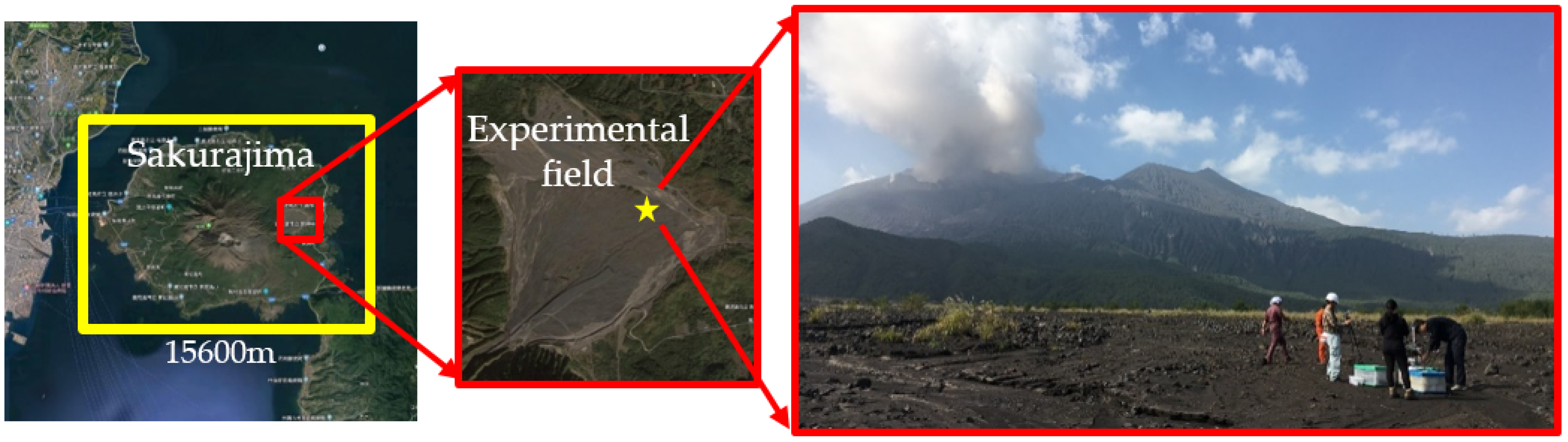
A free fall experiment was carried out in Kurokamijigokugawara, Sakurajima, Kagoshima Prefecture, Japan (Figure 1). There was nothing blocking the view because there were no plants or buildings around. The trajectory of the cinder model falling could be easily obtained and safety was guaranteed.
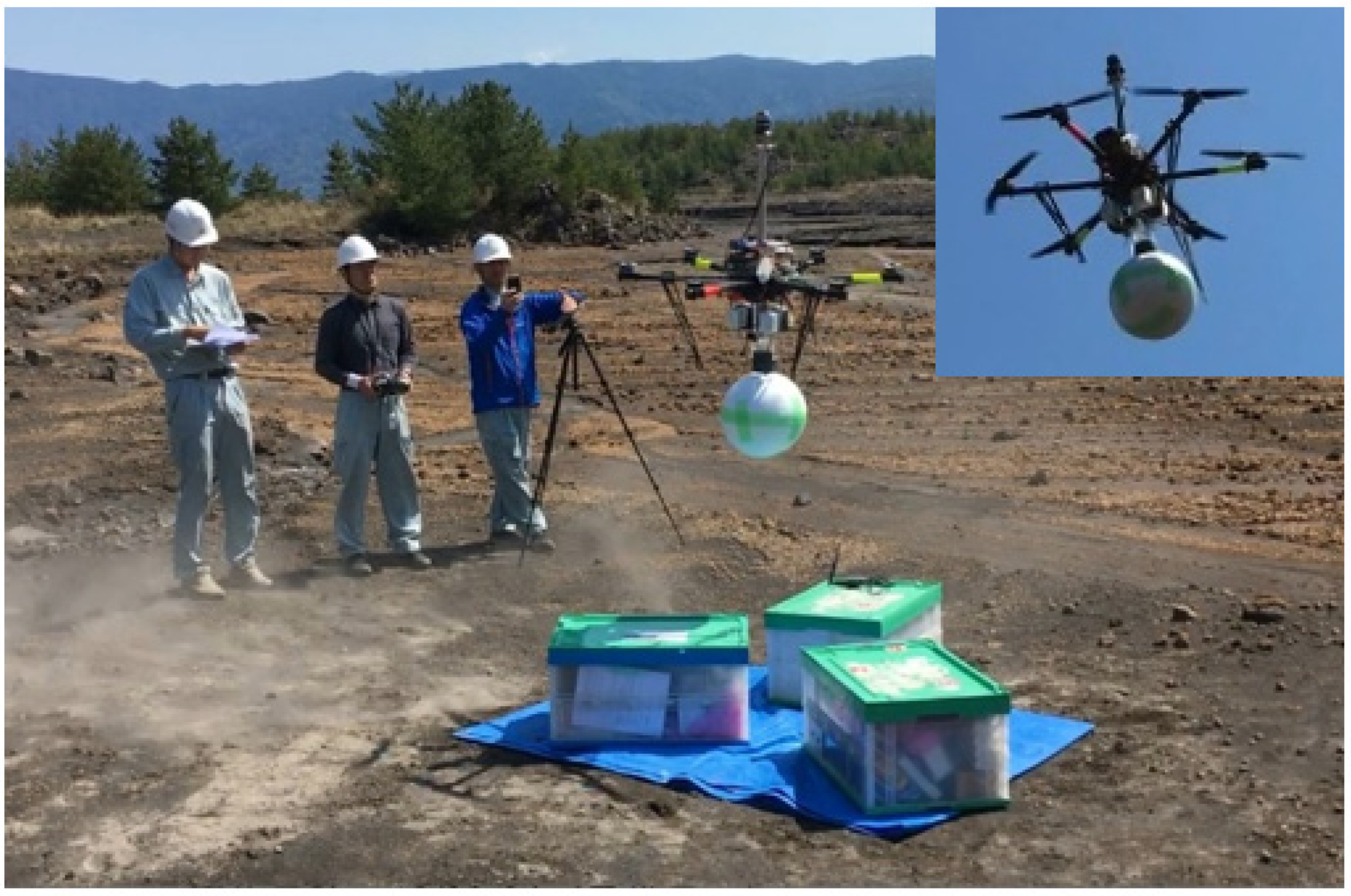
The falling motion of volcanic rocks were measured by using models which imitated the configuration of cinders collected at the site of the experiment. The cinder models were lifted up to an altitude of about 150 m by a drone and dropped as shown in Figure 2. Falling trajectories of the cinder models were recorded by video cameras. Falling motions: acceleration, angular velocity and pressure, were measured by the stand-alone measuring system.
2.2. Cinder Models
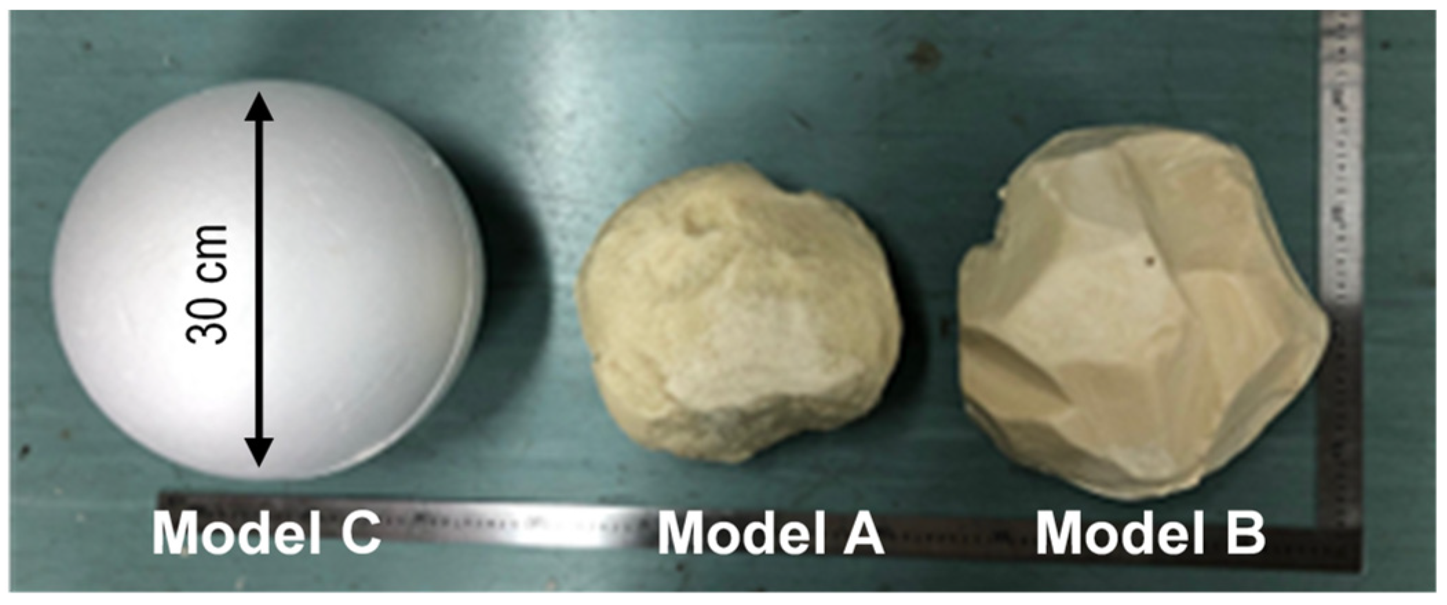
Several shapes were observed in the corrected cinders in the experimental field. After visual inspection, two representative types of shapes were selected for the cinder model. The models imitated the shape of the randomly selected cinders. One has rough texture without sharp edges and its overall shape is relatively smooth, as model A shown in Figure 3. The other, model B, has sharp edges on the surface. We used 3D scanning data of actual cinders to make cinder models. The instantaneous (unaveraged) projected area to the wind direction will be changed when the falling cinder model rotates. This means that our experimental results with six models are equivalent to those using cinder models with various shapes. Cinder models were made of polyurethane foam and were 20 cm to 30 cm in diameter. A sphere, made of polystyrene foam with 30 cm in diameter, was used for comparative verification because lots of information on aerodynamic characteristics were experimented in the previous study. Table 1 shows the specification of the models: model mass, projected area and equivalent diameter, for six test cases. The projected area A was obtained as an averaged value of projected area for overall angle of view. The equivalent diameter L is obtained as .
2.3. Wind Speed
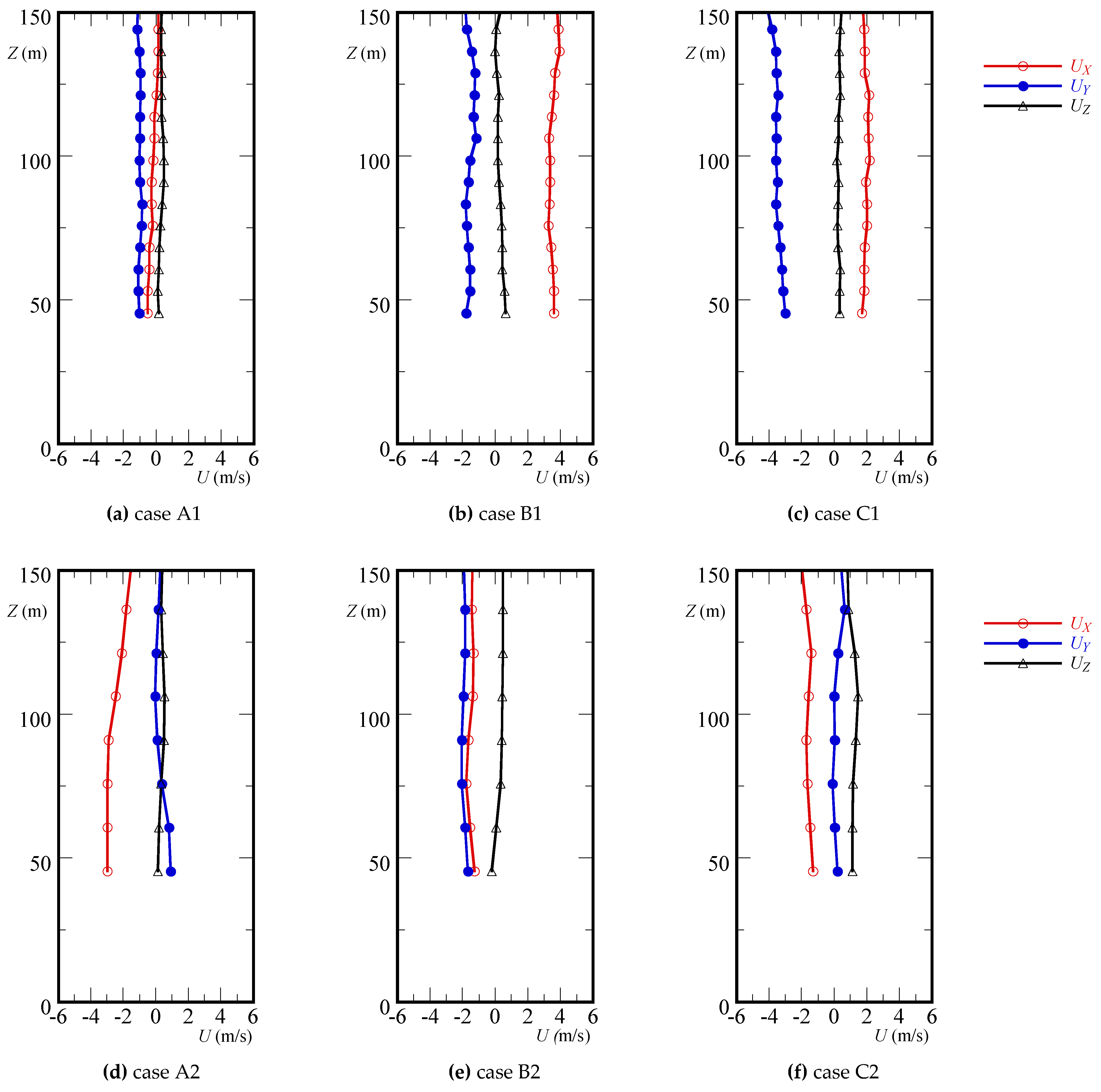
The vertical distribution of wind speed was measured by Doppler lidar (Mitsubishi in Tokyo, Japan, DIABREZZA) during the free fall experiment of all cases as shown in Figure 4. The 20 s mean wind speeds show a gentle breeze condition. These wind speeds are used to calculate the drag coefficient and the deviation angle in Section 3.2. The maximum absolute wind speed of 4 m/s can be found in case B1.
2.4. Measuring Devices
Figure 5 shows the stand-alone measuring system in the cinder model. The system was composed of 3-axis acceleration and angular velocity sensors (Inven Sense in California, USA, MPU-9250), a pressure sensor (Bosch Sensortec in Reutlingen, Germany, GY-BMP280-3.3), a microcomputer board (Raspberry Pi in Cambridge, England, Model A+), an SD memory card, a switch giving an ON/OFF signal of measurement and a battery. Specification of acceleration and angular velocity sensors were shown in Table 2. These measuring devices were put in a box. Rods were attached to the xy-axis of the box so that the measuring devices were fixed in the cinder model. Cotton was stuffed around the box. A hook was attached to the cinder model so that the drone could be easily lifted.
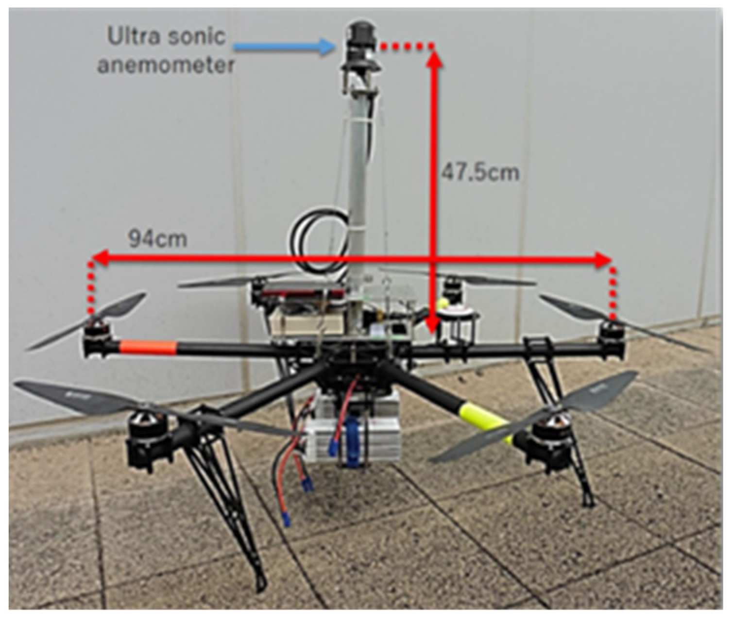
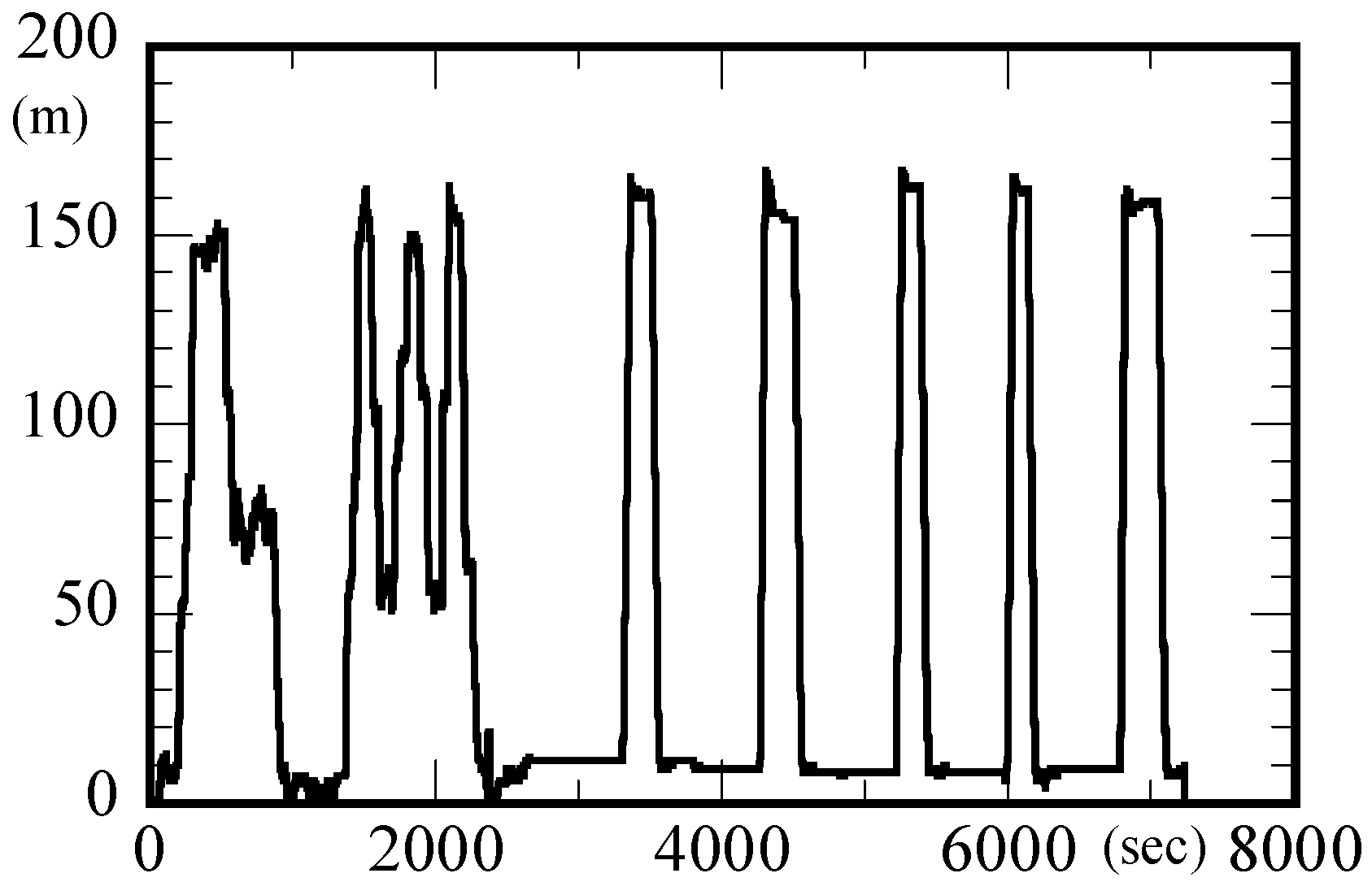
The cinder model was lifted up by a drone (Luce Search in Hiroshima, Japan, SPIDER CS-6) as shown in Figure 6. The drone was equipped with a device for falling model and a smartphone with GPS for recording location. A flight record of drones during the whole day of the experiment shows the altitude of dropping cinder models at about 150 m from the ground as shown in Figure 7.
2.5. Video Motion Analysis
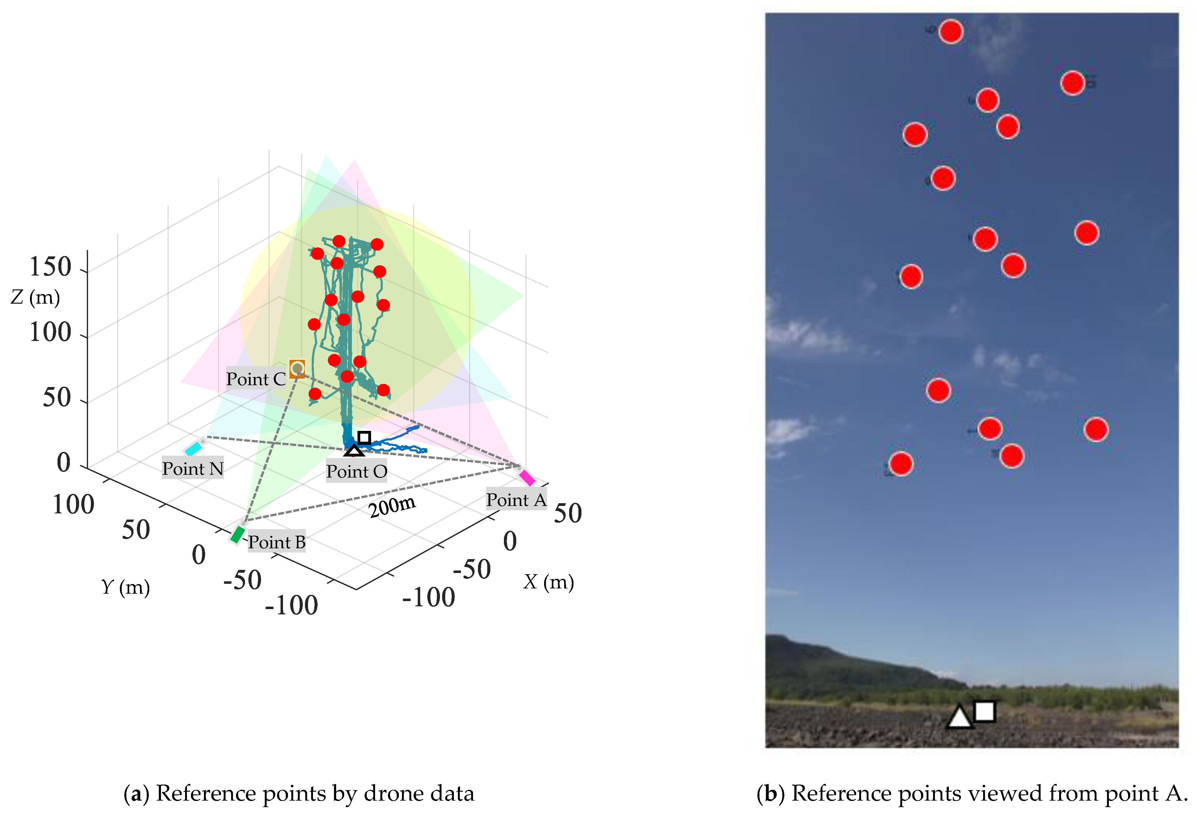
The falling motion of the cinder model was recorded by four video cameras with pixels of 3840 × 2160 and frame rate of 29.97 fps (Panasonic in Osaka, Japan, HC-VX985M). The video cameras were arranged at four points A, B, C and N as shown in Figure 12a. Points A, B and C were located at the vertices of a 200 m triangle. The center of this triangle was point O (the symbol △). The drone flew up from point O to an altitude of 150 m and dropped the cinder model. The view angle of the video camera was adjusted so that all falling motion of the cinder model was within the view of the record. The three-dimensional falling trajectory of the cinder model was calculated from the recorded video view by motion analysis software (DITECT in Tokyo, Japan, Dipp-Motion V). The Direct Linear Transformation method [10] was used as the image analysis algorithm. Previous to the falling experiment, the drone flew to record the reference points shown as red symbols ⬤ in Figure 12a,b because some reference points where the coordinates are known are necessary for the calculation of the trajectory analysis. Both the point O and the location where the cinder model touched down on the ground (the symbol □) were used as reference points.
2.6. Motion Analysis
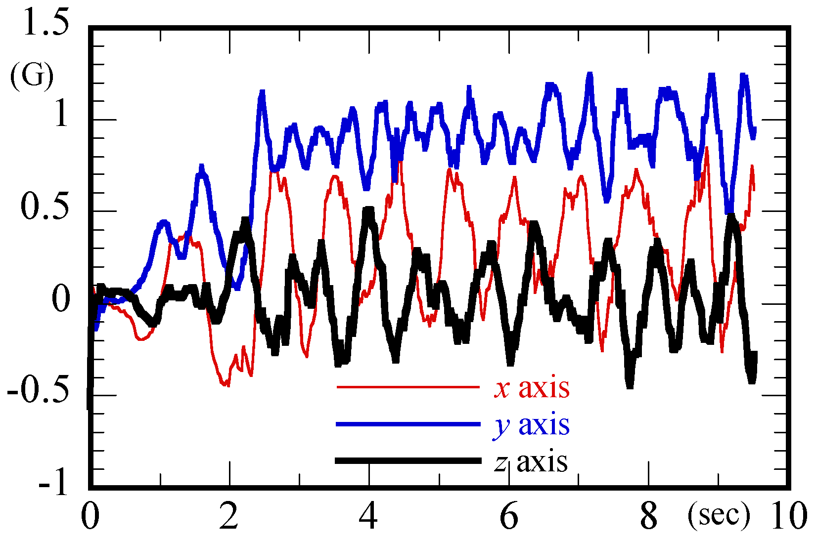
Acceleration and angular velocity in the body coordinate system on the falling model were obtained by the sensors. An example of case A2 was shown in Figure 10 and Figure 11. The bias of angular velocity was corrected. The acceleration and angular velocity were filtered with a 5Hz Butterworth filter.
We converted acceleration and angular velocity into the value in a right-handed absolute coordinate system aligned as X-axis directing to the east, Y-axis to the north and Z-axis to the vertical. The quaternion and the rotation matrix were used for the conversion [11]. Finally, the falling velocity, the displacement and the angle of the falling body were obtained by integration with trapezoidal rule.
The initial posture cannot be determined because the start time of the model falling is uncertain. The initial posture has been optimized so that the trajectory integrated from the record of sensor best matches the trajectory obtained by video analysis.
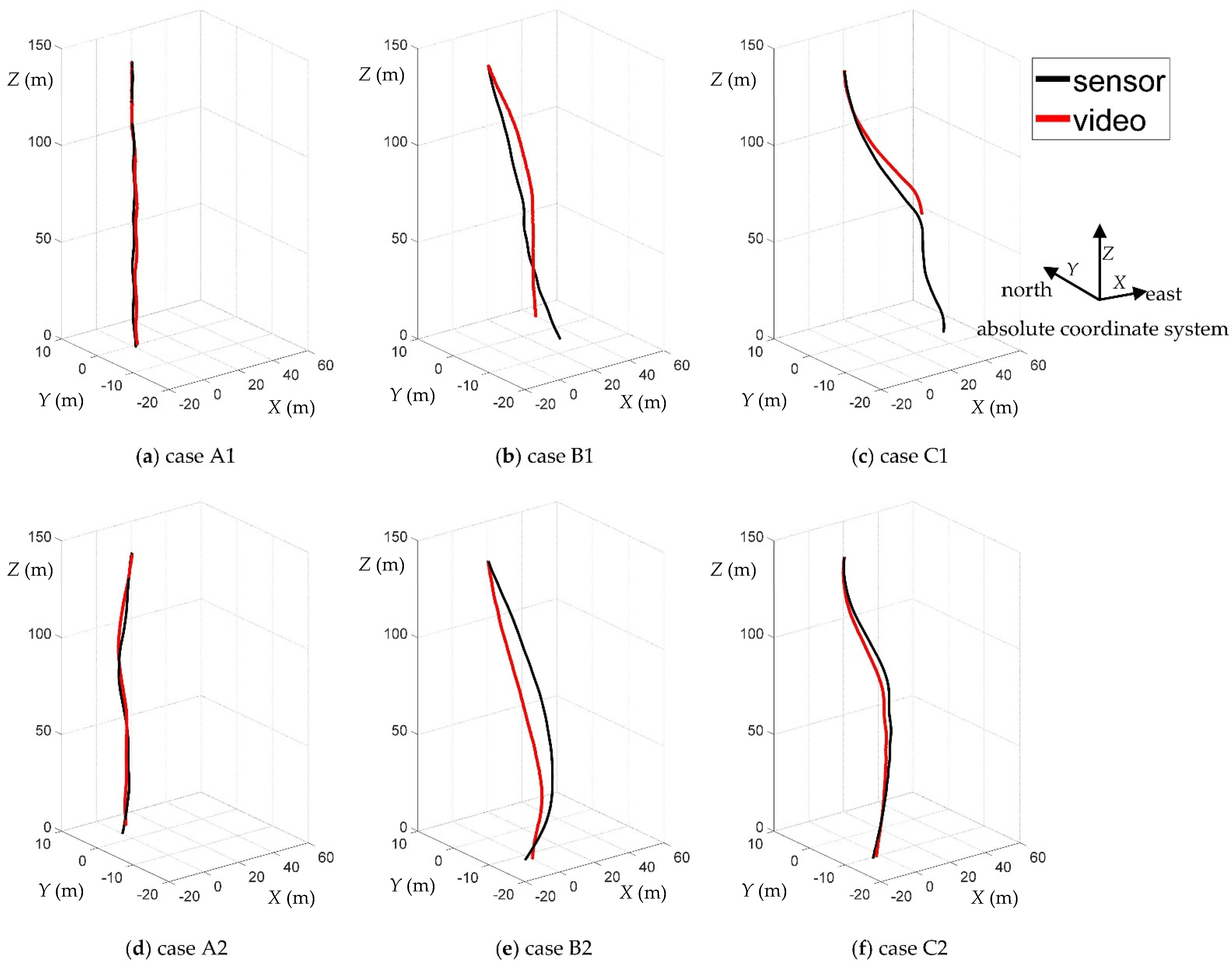
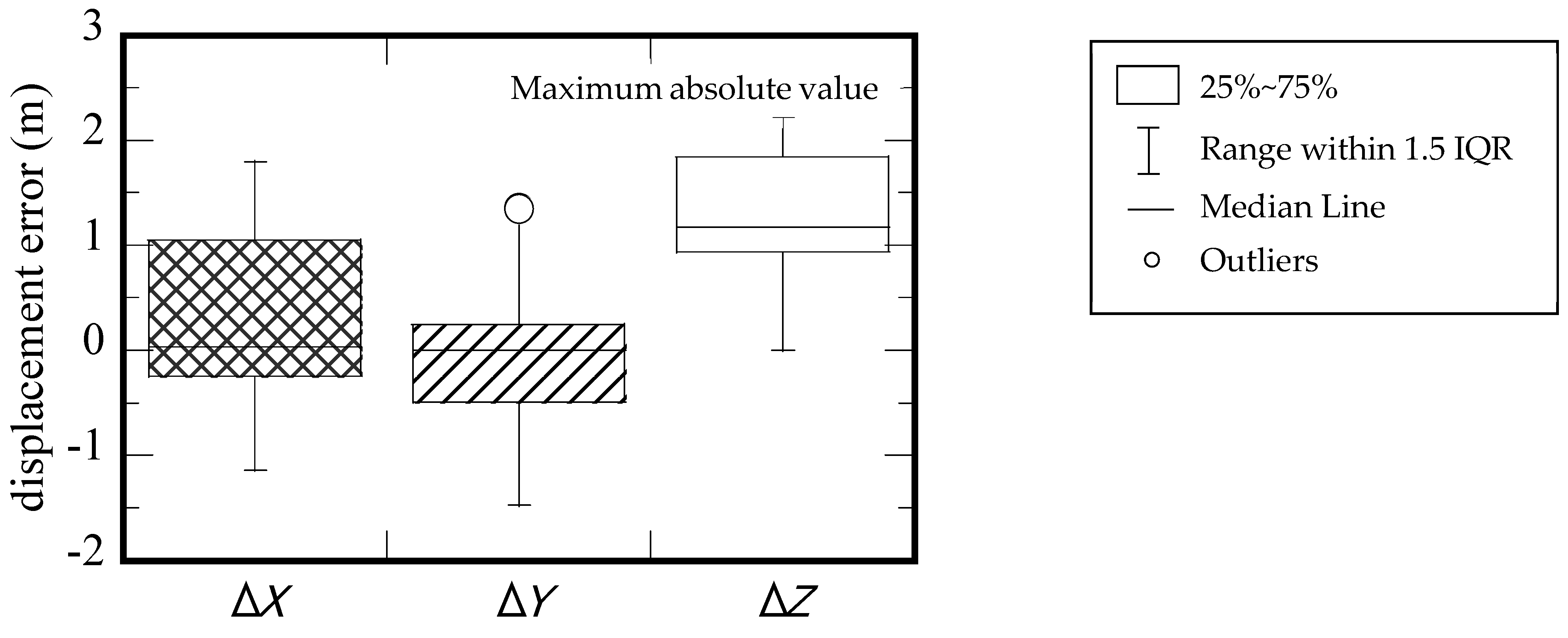
The trajectories obtained by sensor and video analysis in the absolute system are shown in Figure 13. Error of three-axis displacement by sensor and video analysis of all cases are shown in Figure 14. The maximum absolute value of error is about 2.5 m. The error is within 2% with respect to the fall height of 150 m. There are good agreements which ensure the accuracy of the motion analysis. The cinder model went out of the camera view in case C1, so the trajectory by video analysis was broken at the halfway height.
3. Results
3.1. Falling Motion
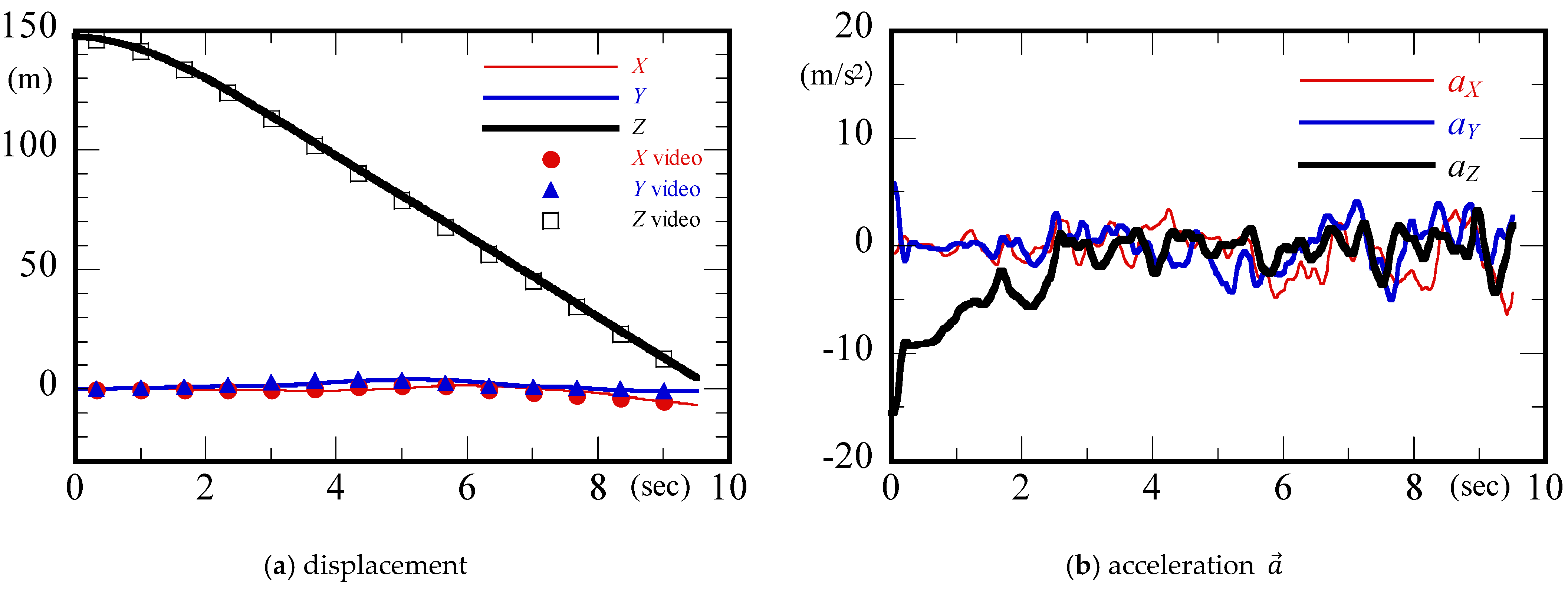
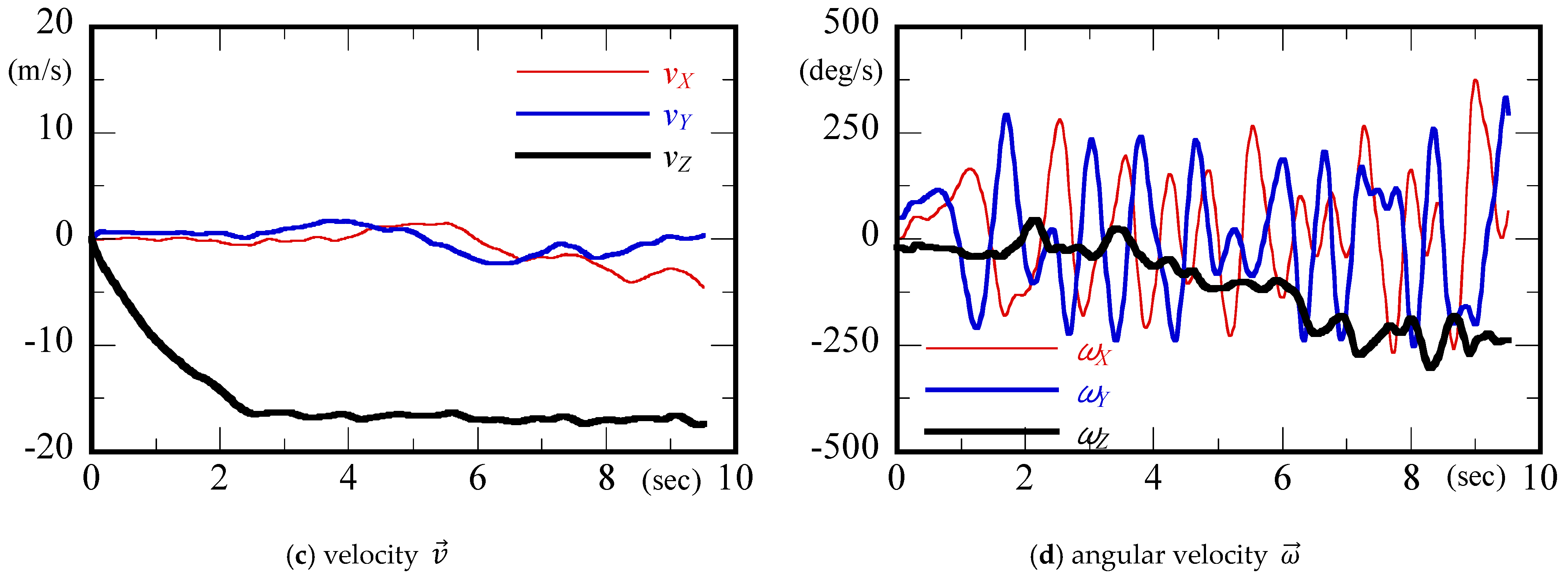
The displacement, acceleration, velocity and angular velocity in the absolute coordinate system were obtained. An example of case A2 is shown in Figure 15. The displacement calculated by sensor shows good agreement with video analysis as shown in Figure 15a. After the falling, the vertical acceleration : z component increased and was around 0 m/s2 after 3 s as shown in Figure 15b. This means that the wind resistance on the cinder model increased and balanced with the gravity, and the velocity reached terminal velocity: −17 m/s, at 2.5 s as shown in Figure 15c. The magnitude of angular velocity of the vertical component gradually increased after 4 s as shown in Figure 15d. The periodic variation of X and Y components of angular velocity and showed the precession along the Z axis.
3.2. Drag Coefficient and Deviation Angle
We derived the wind resistance force from the acceleration as
where m is the mass and g is the gravitational acceleration as 9.794 m/s2. The drag coefficient was derived as
where A is the projected area of the falling body and the dynamic pressure is defined as
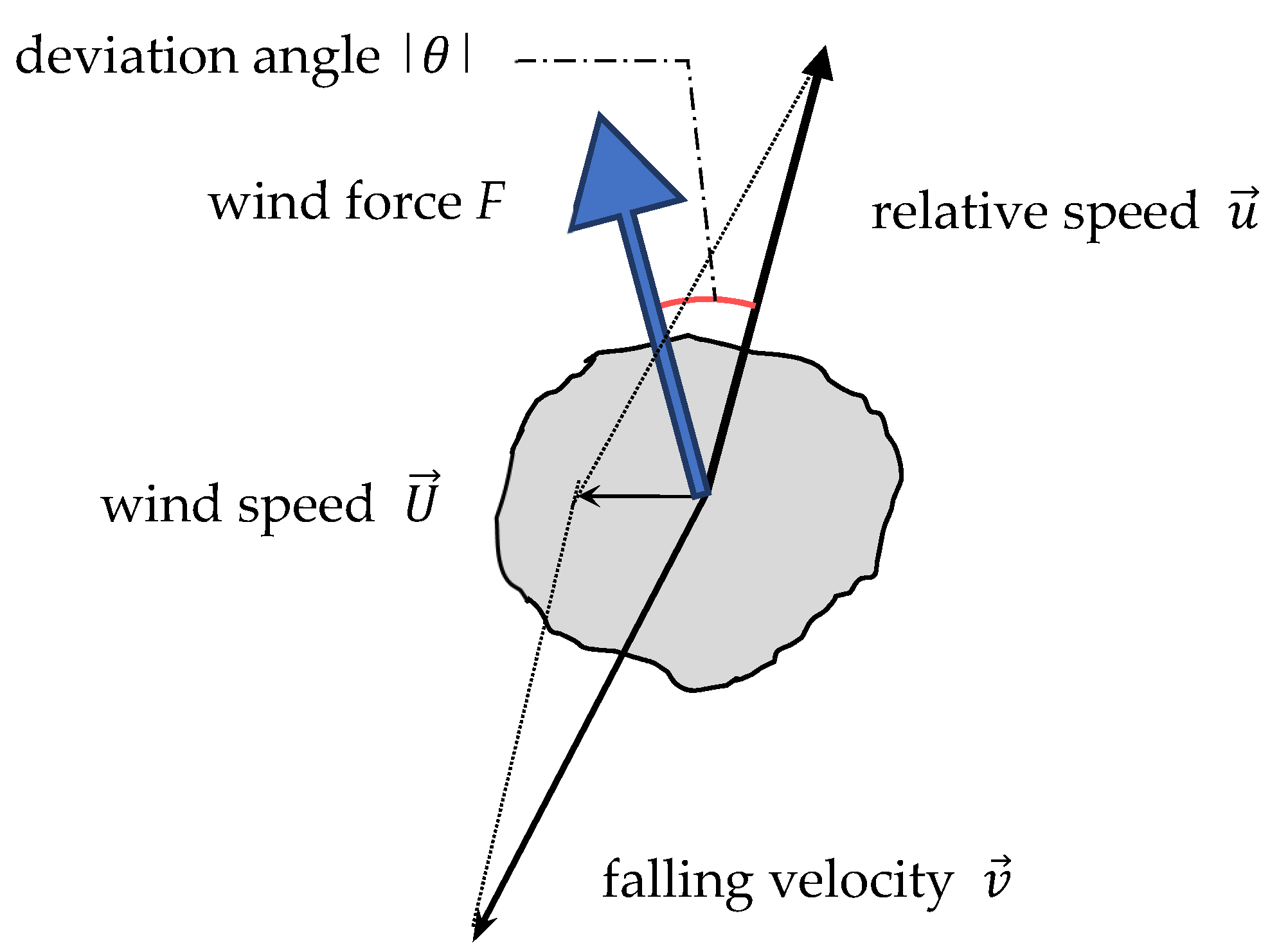
where is the air density as 1.2 kg/m3 and is the relative velocity defined as the difference of the wind speed and the velocity of falling body :
As shown in Figure 16. The Doppler lidar cannot measure wind speed below 50 m. So the wind speed at 50 m was used for the calculation below 50 m.
The deviation angle between wind direction and wind resistant force direction was derived as
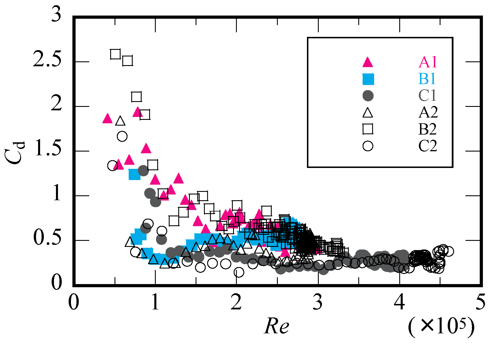
Figure 17 shows the variation of drag coefficient with Reynolds number for different test cases, where is the representative length shown in Table 1 and is the air viscosity as 1.8 10−5 Pa·s. varies with the configuration of the cinder models in the range of low . Also varies with the falling motion because the instantaneous projected area to the wind direction is changed. The dispersion of decreases with and may converge to a constant value of around 0.4 that is a little bit larger than that of sphere.
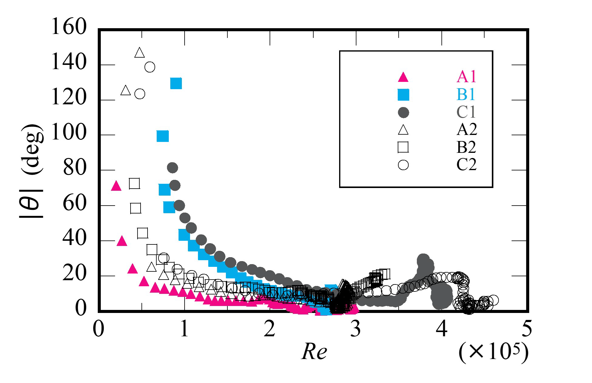
The deviation angle varies with configuration of the cinder models and the instantaneous projected area to the wind direction as shown in Figure 18. The magnitude and dispersion of decrease with the Reynolds number . In the range of high , of the cinder model varies within 22 degrees, independent of . Otherwise of the sphere varies within 31 degrees.
4. Discussion
To do ballistic simulation, we need to know magnitude and direction of wind force of the cinder. There are various shapes of actual cinders. The magnitude and direction of wind force varies with configuration of the shapes and the instantaneous projected area of the wind. The projected area will be changed when the falling cinder model rotates. This means that our experimental results with six models include results of used cinder models with various shapes. The magnitude and direction of wind force can be calculated by the drag coefficient and deviation angle obtained in our study.
The drag coefficient and deviation angle varies with the cinder configuration and the instantaneous projected area with rotation of the cinder. The magnitude and dispersion of and decrease with the Reynolds number as obtained in this study.
The results of and in this study include the effect of cinder model rotation. Therefore, the ballistic simulation with them includes the effect of rotation. We can calculate the trajectory without calculating the dynamics of rotation.
The variations of and do not show obvious dispersion at the same , so we may use the constant frequency distribution for and . We will try to have further study on this point.
5. Conclusions
We conducted the free fall experiment from a drone using cinder models. Falling motion of the cinder models were recorded by video camera and a stand-alone measuring system that was assembled with a pressure sensor, acceleration and angular velocity sensors in the cinder models. Three-dimensional falling trajectory and motion, including displacement, acceleration, velocity and angular velocity, were calculated. The variation of the drag coefficient and the deviation angle with Reynolds number were obtained.
The drag coefficient varies with the configurations of falling body and the falling motion when the Reynolds number is small. The drag coefficient converges into 0.4 that is a little bit larger than that of sphere’s value when the Reynolds number is large. The deviation angle of cinder model is within 22 degrees independent of the configurations; that of the sphere varies within 31 degrees when Reynolds number is large.
To do ballistic simulation, it is necessary to determine the frequency distribution of the drag coefficient and deviation angle at the same Reynolds number. We may use the constant frequency distribution for the drag coefficient and deviation angle at the same Reynolds number because the variations of drag coefficient and deviation angle show no obvious dispersion.
The ballistic simulation with the drag coefficient and deviation angle obtained include effect of rotation. It will be convenient to calculate ballistic trajectory without calculating the dynamics of rotation.
Author Contributions
Conceptualization, M.L. and T.M.; methodology, M.L. and T.M.; validation, M.L., T.M., M.I. (Masato Iguchi); formal analysis, M.L.; investigation, M.L. and T.M.; data curation, K.S., M.I. (Minoru Inoue); writing—original draft preparation, M.L.; writing—review and editing, T.M., M.I. (Masato Iguchi) and E.F.; visualization, M.L.; supervision, T.M.; project administration, T.M.; funding acquisition, M.I. (Masato Iguchi) and E.F. All authors have read and agreed to the published version of the manuscript.
Funding
This research was funded by 2019 General Collaborative Research with the Disaster Prevention Research Institute of Kyoto University, grant number 30G-10 and was funded by MEXT Next Generation Volcano Research Program Grant Number JPJ005391.
Institutional Review Board Statement
Not applicable.
Informed Consent Statement
Not applicable.
Data Availability Statement
Not applicable.
Acknowledgments
This work was supported by MEXT Next Generation Volcano Research Program Grant Number JPJ005391. T. Komiya, K. Takishita, I. Yoneda, T. Yamazaki, M. Kamo, K. Doi for helping the experiment. T. Shimura, T. Yoda, H. Ninomiya for operating the drone. H. Nishimura for designing of the measuring system. The authors would like to thank anonymous reviewers for their supportive and insightful comments that helped improved the manuscript.
Conflicts of Interest
The authors declare no conflict of interest.
References
- Oikawa, T.; Yamaoka, K.; Yoshimoto, M.; Nakada, S.; Takeshita, Y.; Maeno, F.; Ishizuka, Y.; Komori, J.; Shimano, T.; Nakano, S. The 2014 Eruption of Ontake Volcano, Central Japan. Volcanol. Soc. Jpn. 2015, 60, 411–415. (In Japanese) [Google Scholar]
- Bower, S.M.; Woods, A.W. On the dispersal of clasts from volcanic craters during small explosive eruptions. J. Volcanol. Geotherm. Res. 1996, 73, 19–32. [Google Scholar] [CrossRef]
- Iguchi, M.; Kamo, K. On the range of block and lapilli ejected by the volcanic explosions. Disaster Prev. Res. Inst. Annu. B 1984, 27, 15–27. (In Japanese) [Google Scholar]
- Steinberg, G.S.; Babenko, J.I. Experimental velocity and density determination of volcanic gases during eruption. J. Volcanol. Geotherm. Res. 1978, 3, 89–98. [Google Scholar] [CrossRef]
- Alatorre-Ibargüengoitia, M.A.; Delgado-Granados, H. Experimental determination of drag coefficient for volcanic materials: Calibration and application of a model to Popocatépetl volcano (Mexico) ballistic projectiles. Geophys. Res. Lett. 2006, 33, 11. [Google Scholar] [CrossRef]
- Tachikawa, M. Trajectories of flat plates in uniform flow with application to wind-generated missiles. J. Wind Eng. Ind. Aerodyn. 1983, 14, 443–453. [Google Scholar] [CrossRef]
- Okazaki, J.; Maruyama, T. Simulation of roof tile and square flat plate scattering in wind. In Proceedings of the 22nd National Symposium on Wind Engineering, Tokyo, Japan, 5–7 December 2012; pp. 377–382. (In Japanese). [Google Scholar] [CrossRef]
- Richards, P.J.; Williams, N.; Laing, B.; McCarty, M.; Pond, M. Numerical calculation of the three-dimensional motion of wind-borne debris. J. Wind Eng. Ind. Aerodyn. 2008, 96, 2188–2202. [Google Scholar] [CrossRef]
- Matsui, K.; Maruyama, T.; Nishimura, H.; Noda, H. Direct Measurement of Aerodynamic Characteristics of Flying Debris Models by Stand-Alone Measuring Device. Proceedings of the 25th National Symposium on Wind Engineering 169–174. (In Japanese) [CrossRef]
- Shapiro, R. Direct linear transformation method for three-dimensional cinematography. Res. Q. Am. Alliance Health Phys. Educ. Recreat. 1978, 49, 197–205. [Google Scholar] [CrossRef]
- Cooke, J.M.; Zyda, M.J.; Pratt, D.R.; McGhee, R.B. NPSNET: Flight Simulation Dynamic Modeling Using Quaternions. Presence Teleoperators Virtual Environ. 1992, 1, 404–420. [Google Scholar] [CrossRef]
Figure 1.
Experimental field.

Figure 2.
State of lifting a model by drone.

Figure 3.
Cinder models: A and B, and a sphere: C.

Figure 4.
Three-axis mean wind speed of all test cases: (a) case A1; (b) case B1; (c) case C1; (d) case A2; (e) case B2; (f) case C2.
Figure 4.
Three-axis mean wind speed of all test cases: (a) case A1; (b) case B1; (c) case C1; (d) case A2; (e) case B2; (f) case C2.

Figure 5.
Stand-alone measuring system in the cinder model.

Figure 6.
Drone used for experiment.

Figure 7.
Flight record of vertical elevation by GPS.

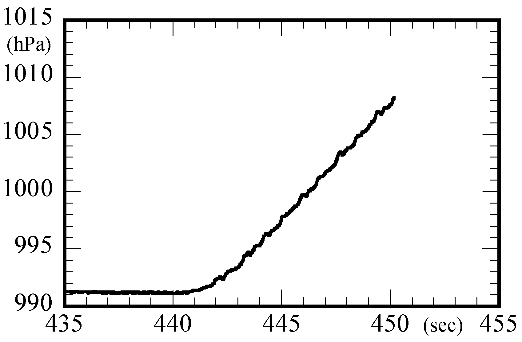
Figure 8.
Time history of pressure sensor record of case A2.

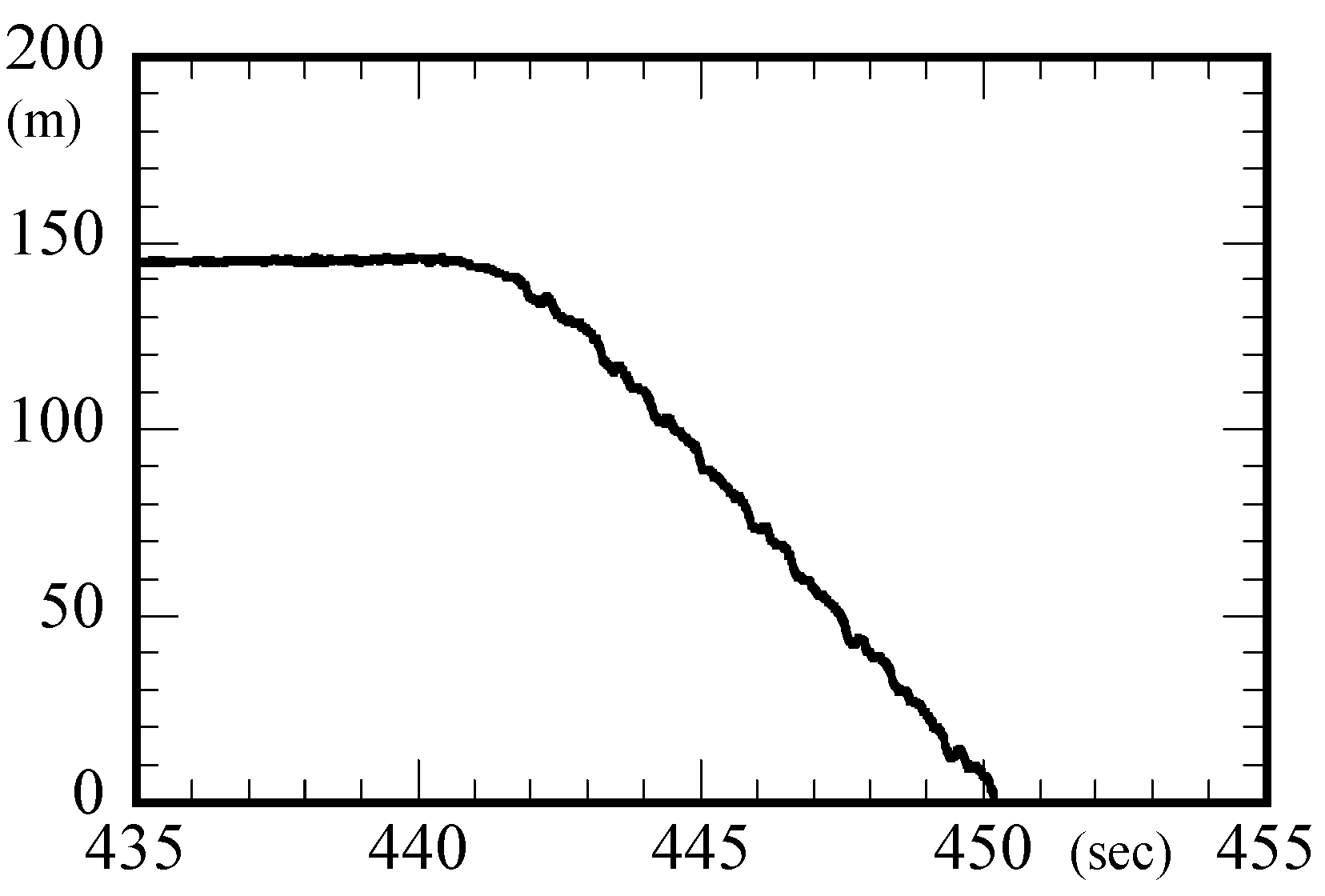
Figure 9.
Vertical elevation converted from pressure sensor record in Figure 8.
Figure 9.
Vertical elevation converted from pressure sensor record in Figure 8.

Figure 10.
Acceleration recorded by the sensor in the body coordinate system of case A2.

Figure 11.
Angular velocity recorded by the sensor in the body coordinate system of case A2.

Figure 12.
Reference points for video analysis: (a) reference points by drone data; (b) reference points viewed from point A. Points A, B, C and N in Figure 12a were the camera’s positions. Bule lines in Figure 12a indicates the drone flight trajectory. Point O in Figure 12a: △ indicates the center of points A, B and C. □ in Figure 12a,b indicates location where the cinder model touched down on the ground. ⬤, △, □ in Figure 12a,b were used as reference points.

Figure 13.
Trajectories obtained by sensor and video analysis of all test cases: (a) case A1; (b) case B1; (c) case C1; (d) case A2; (e) case B2; (f) case C2.
Figure 13.
Trajectories obtained by sensor and video analysis of all test cases: (a) case A1; (b) case B1; (c) case C1; (d) case A2; (e) case B2; (f) case C2.

Figure 14.
Box plots of median and interquartile range (IQR) for 3-aixs displacement error (ΔX, ΔY, ΔZ) by internal sensors and external camera observation of all cases.
Figure 14.
Box plots of median and interquartile range (IQR) for 3-aixs displacement error (ΔX, ΔY, ΔZ) by internal sensors and external camera observation of all cases.

Figure 15.
Calculated motion with sensor’s record of case A2: (a) displacement; (b) acceleration; (c) velocity; (d) angular velocity.
Figure 15.
Calculated motion with sensor’s record of case A2: (a) displacement; (b) acceleration; (c) velocity; (d) angular velocity.


Figure 16.
Definition of relative velocity and deviation angle .

Figure 17.
Variation of drag coefficient with Reynolds number.

Figure 18.
Variation of deviation angle with Reynolds number. Note that unit of θ in Equation (5) is the radian. Unit of y-axis θ in Figure 18 is the degree.
Figure 18.
Variation of deviation angle with Reynolds number. Note that unit of θ in Equation (5) is the radian. Unit of y-axis θ in Figure 18 is the degree.


Table 1.
Mass m, projected area A and equivalent diameter L of six test cases.
| Case | Model Type | m (kg) | A (m2) | L (m) |
|---|---|---|---|---|
| A1 | A | 0.41 | 0.048 | 0.25 |
| B1 | B | 0.42 | 0.054 | 0.26 |
| C1 | C | 0.39 | 0.071 | 0.30 |
| A2 | A | 0.41 | 0.048 | 0.25 |
| B2 | B | 0.46 | 0.054 | 0.26 |
| C2 | C | 0.47 | 0.071 | 0.30 |
Table 2.
Specification of acceleration and angular velocity sensors.
| Acceleration Sensor | Angular Velocity Sensor | |
|---|---|---|
| Sampling frequency | 50 Hz | |
| Measurement range | ±8 g | ±1000°/s |
| AD converter | 16 bit | |
| Power supply voltage | DC2.4 V~3.6 V | |
| Size | 13 mm × 11 mm | |
Publisher’s Note: MDPI stays neutral with regard to jurisdictional claims in published maps and institutional affiliations. |
© 2021 by the authors. Licensee MDPI, Basel, Switzerland. This article is an open access article distributed under the terms and conditions of the Creative Commons Attribution (CC BY) license (https://creativecommons.org/licenses/by/4.0/).
Share and Cite
MDPI and ACS Style
Liu, M.; Maruyama, T.; Sasaki, K.; Inoue, M.; Iguchi, M.; Fujita, E. Measurement of Aerodynamic Characteristics Using Cinder Models through Free Fall Experiment. Atmosphere 2021, 12, 608. https://doi.org/10.3390/atmos12050608
AMA Style
Liu M, Maruyama T, Sasaki K, Inoue M, Iguchi M, Fujita E. Measurement of Aerodynamic Characteristics Using Cinder Models through Free Fall Experiment. Atmosphere. 2021; 12(5):608. https://doi.org/10.3390/atmos12050608
Chicago/Turabian StyleLiu, Meizhi, Takashi Maruyama, Kansuke Sasaki, Minoru Inoue, Masato Iguchi, and Eisuke Fujita. 2021. "Measurement of Aerodynamic Characteristics Using Cinder Models through Free Fall Experiment" Atmosphere 12, no. 5: 608. https://doi.org/10.3390/atmos12050608
Note that from the first issue of 2016, this journal uses article numbers instead of page numbers. See further details here.