
Nocturnal Boundary Layer Evolution and Its Impacts on the Vertical Distributions of Pollutant Particulate Matter


1
Institute of Atmospheric Physics, Chinese Academy of Sciences, Beijing 100029, China
2
University of Chinese Academy of Sciences, Beijing 100049, China
3
Key Laboratory of Environmental Optics and Technology, Anhui Institute of Optics and Fine Mechanics, Chinese Academy of Sciences, Hefei 230031, China
4
Shanghai Environmental Monitoring Center, Shanghai 200235, China
*
Author to whom correspondence should be addressed.
Atmosphere 2021, 12(5), 610; https://doi.org/10.3390/atmos12050610
Submission received: 12 April 2021
/
Revised: 30 April 2021
/
Accepted: 4 May 2021
/
Published: 7 May 2021
(This article belongs to the Special Issue Aerosol Pollution in Asia)
Abstract
:To investigate the evolution of the nocturnal boundary layer (NBL) and its impacts on the vertical distributions of pollutant particulates, a combination of in situ observations from a large tethered balloon, remote sensing instruments (aerosol lidar and Doppler wind lidar) and an atmospheric environment-monitoring vehicle were utilized. The observation site was approximately 100 km southwest of Beijing, the capital of China. Results show that a considerable proportion of pollutant particulates were still suspended in the residual layer (RL) (e.g., the nitrate concentration reached 30 μg m−3) after sunset. The NBL height calculated by the aerosol lidar was closer to the top of the RL before midnight because of the pollutants stored aloft in the RL and the shallow surface inversion layer; after midnight, the NBL height was more consistent with the top of the surface inversion layer. As the convective mixing layer gradually became established after sunrise the following day, the pollutants stored in the nocturnal RL of the preceding night were entrained downward into the mixing layer. The early morning PM2.5 concentration near 700 m in the RL on 20 December decreased by 83% compared with the concentration at 13:34 on 20 December at the same height. The nitrate concentration also decreased significantly in the RL, and the mixing down of nitrate from the RL could contribute about 37% to the nitrate in the mixing layer. Turbulence activities still existed in the RL with the bulk Richardson number (Rb) below the threshold value. The corresponding increase in PM2.5 was likely to be correlated with the weak turbulence in the RL in the early morning.
1. Introduction
Rapid urbanization, industrial production and economic activities have led to increased emissions of pollutants into the atmosphere, and in recent years, pollution events in Asia have occurred frequently [1,2,3,4]. Atmospheric pollutants are concentrated mainly within the planetary boundary layer (PBL), that is, the atmospheric layer 1–2 km above the ground, sometimes as high as 3 km [5]. Generally speaking, without the consideration of large-scale advection, subsidence processes and any special underlying surface, such as the polar region, the daytime PBL is also called the convective boundary layer (CBL), characterized by strong vertical mixing [5]. However, with the gradual formation of a surface inversion layer near the ground due to strong surface radiative cooling after sunset, the CBL transforms into the nocturnal boundary layer (NBL) consisting of the stable boundary layer (SBL), the residual layer (RL), and a capping inversion layer separating the entire NBL from the free atmosphere [6]. The RL is situated above the stable boundary layer (SBL) because the initial mean state variables and concentration variables of the RL are the same as those of the previously decayed mixing layer [5,7].
In recent years, considerable research has been performed to study the dispersion of air pollutants and the corresponding physicochemical processes in the atmosphere [8,9,10,11,12,13,14]. However, relatively little attention has been paid to the NBL, especially the RL, in which the dispersion of contaminants occurs under conditions of decaying turbulence. In addition to advective transport and local high-emission sources, the importance of the effect the RL has on pollution cannot be ignored considering the rapid and explosive growth of pollutant particles over a short time. Research on the evolution of the NBL requires detecting the vertical structure of the PBL; unfortunately, compared with continuous surface observations, vertical observations of the PBL are more difficult and challenging to acquire. Nevertheless, over the last 30 years, continuous advancements in atmospheric vertical measurement techniques have provided favorable conditions and possibilities for the analysis of NBL properties [15,16].
High meteorological towers hold many advantages, but their detection height is very limited. Consequently, it is difficult to obtain information regarding the vertical physicochemical distribution during the evolution of the NBL. Aircraft observations can also be utilized to directly image the vertical profile of the PBL above a certain region; accordingly, many field experiments have been carried out [17], confirming the formation of new particles at the top of the PBL [1]. Aircraft observations conducted in America have shown that the nocturnal RL can affect the ground-level ozone concentration on the following day [18], especially in the early morning, when the surface inversion layer gradually dissipates. The contribution ratio of this mechanism was further assessed [19]. However, aircraft cannot fly at low altitudes (<1000 m) and are strongly limited by the allowable airspace. In recent years, atmospheric remote sensing technologies, such as aerosol lidar, Doppler lidar and telescopes have developed greatly; these technologies can overcome the drawbacks of near-ground monitoring networks to a certain extent [20,21,22] and can continuously monitor the vertical distributions of pollutants and meteorological elements as well as optical characteristics in the PBL [23,24,25,26]. Remote sensing has been widely used in environmental protection because of its high spatial resolution and continuous measurement ability [27,28]. Aerosol lidars retrieve atmospheric extinction coefficients and depolarization ratios by receiving aerosol particle backscattering signals. As a result, aerosol lidars have been used extensively to retrieve and analyze the evolutionary characteristics of the PBL height [27,29,30]. Aerosol lidar signals are unreliable below 150 m because of the incomplete transmitter–receiver overlap, and remote sensing observation data need strict quality control. At present, particulates still constitute the main detection objectives of lidars; ozone lidar and nitrogen oxide lidar are gradually being promoted [31]. Lidar cannot effectively distinguish among atmospheric pollutant components and thus cannot be used to identify chemical processes in pollutants [32]. However, aerosol lidars can directly reflect the atmospheric pollutants suspended in the RL, and thus, studies have employed lidar technologies to investigate the formation of new particles within the RL [33].
Observations acquired from a tethered balloon have considerable advantages because such balloons can carry a variety of measurement instruments, thereby achieving the simultaneous observation of multiple parameters [34,35] and directly obtaining the vertical distributions of physicochemical properties in the lower PBL. Tethered balloon observation experiments were conducted in Shanghai [11], a coastal megacity in eastern China, while focusing on the ozone concentration [36]. Some experiments have also been implemented in North China to observe the variations in the vertical distributions of pollutants by tethered balloons [37,38,39]; however, these investigations were limited to the size of the tethered balloon, and they did not pay sufficient attention to the important role that the nocturnal RL plays in the accumulation of pollutants.
An increasing number of studies have reported that the NBL can affect air quality through vertical mixing processes [7,40], but most of these studies focused on ozone problems [41]. However, pollutant particulates, especially secondary aerosol particulates, are very important because secondary pollutants account for nearly 70% of the pollution during heavy pollution episodes in North China [39]. Synchronous observation of the vertical profiles of pollutant particulate and meteorological parameters in North China are relatively scarce. The influences of the evolution of NBL on the vertical distributions of pollutant particulates are seldom discussed.
This paper discusses and analyzes the evolution of the NBL and its impacts on the vertical distributions of pollutant particulate matter, especially secondary aerosol particulates, from the perspective of the complete PBL diurnal variation. The remainder of this paper is organized as follows: the measurement site and instrumentation are introduced in Section 2, the impacts of the NBL on the vertical distribution of pollutants are presented in Section 3, and the main conclusions are provided in Section 4.
2. Measurement Site and Instrumentation
2.1. Field Experiment
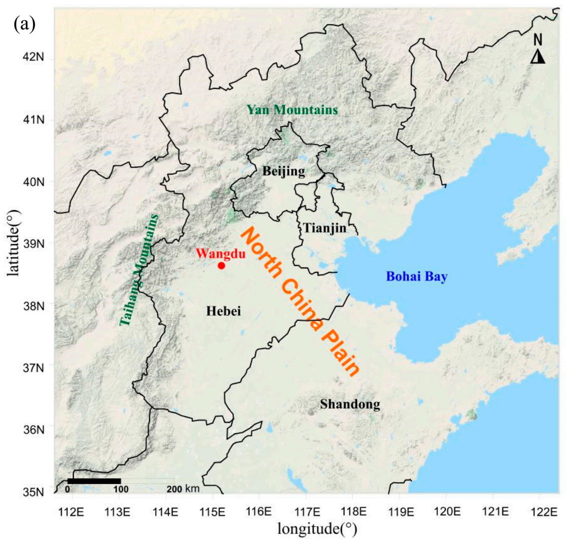
A comprehensive and intensive observation experiment, organized and managed by the China National Key Research and Development Program entitled “Vertical Detection Technology of Air Pollution in the Continental Atmospheric Boundary Layer”, was conducted in Wangdu County, Hebei Province of North China (about 100 km southwest of Beijing, the capital of China, as shown in Figure 1a). It is situated along the waterfront in the piedmont along the Taihang Mountains and belongs to a cluster of cities in the North China Plain (NCP). Its geographical location is illustrated in Figure 1a. Wangdu is surrounded by mountains on three sides, similar to Beijing, and is 44 m above sea level. The comprehensive PBL pollution observation experiment performed in Wangdu helped to characterize the pollution events in the NCP area and to reveal their formation mechanism. Figure 1b shows the specific measurement site (115.25° E, 38.66° N) in Wangdu County; the flat terrain of the observation site provided horizontally homogeneous conditions. The local air pollutant emission sources surrounding the Wangdu experiment site originated mainly from agricultural combustion, traffic emissions, and residential production, but no direct obvious industry sources nearby were present.
The large tethered balloon platform used in this experiment was 1900 m3 in volume; its maximum carrying weight was 200 kg, and its detection altitude was 1000 m (shown in Figure 1b). A variety of instruments attached to the tethered balloon included the instrument (MAS-AF300, Homo Sapiens, Shenzhen, China) measuring the concentrations of PM1, PM2.5 and PM10 with a time resolution of 1 min, and a quadrupole aerosol chemical speciation monitor (Q-ACSM, Aerodyne Research, Billerica, MA, USA), which measured the concentrations of secondary inorganic aerosol particles, namely, sulfates, nitrates and ammonium salts. Organic (Org) compounds were also measured. Portable meteorological stations (HC2-S, Rotronic, Bassersdorf, Switzerland) measuring temperature and relative humidity were also equipped on the balloon platform. Tethered balloon observations require a relatively low horizontal wind speed (<3 m s−1) to ensure that the ascension and descension rates of the balloon are steady with a speed of 0.5 m s−1 by means of an electrical winch. The shape of the tethered balloon used in this experiment was similar to an airship configuration and was streamlined to reduce aerodynamic drag. A global positioning system (GPS) sensor was also mounted on the tethered balloon, providing real-time longitude, latitude and altitude information.
Simultaneously, the PBL structure was detected continuously by ground-based remote sensing instruments such as an aerosol lidar (AGHJ-I-lidar, Zhongke Guangdian, Wuxi, China) and a Doppler wind lidar (FC-II, Norinco Group, Beijing, China). The aerosol lidar provided backscattering signals at a vertical resolution of 7.5 m and a temporal resolution of approximately 5–10 min. The Doppler wind lidar was used to retrieve wind profiles and had a spatial resolution of 50 m and a time resolution of 2–3 s.
Furthermore, pollutant concentrations (e.g., O3, SO2 and CO) and meteorological parameters on the ground during the observation period were monitored by a mobile monitoring vehicle. The experiment was also carried out in tandem with aircraft sampling. Overall, the experiment, which utilized multiple detection platforms, consisted of large-scale multi-platform and multi-element observations of the PBL in the NCP area. In [42] the detection accuracy of various instruments used in this paper has been listed.
Frequent ascents and descents of a tethered balloon enable the evolution of the vertical PBL structure to be studied. In this paper, observation data acquired from the tethered balloon, ground-based aerosol lidar, Doppler wind lidar and ground measurement instruments from 10:00 on 19 December 2018, to 14:00 on 20 December 2018 (local time was used in this paper), were used and analyzed. In addition, twice-daily (08:00 and 20:00) routine radiosonde observations were also recorded at station 54511; these data can provide information on the vertical profiles of meteorological factors such as wind and temperature and pollutant particulates in the PBL. There were few clouds during the observation period. The PBL exhibits obvious diurnal variation; according to the local sunrise (07:30) and sunset (17:00) times in winter; the three stages in this paper are classified as follows: Stage 1, 10:00 to 17:00 on 19 December 2018, the evolution from a CBL to an NBL with an emerging RL; Stage 2, from 17:00 on 19 December 2018 to 07:30 on 20 December 2018, after sunset, when the SBL gradually develops until sunrise the following day, leaving a morning RL; and Stage 3, from 07:30 to 14:00 on 20 December 2018, the daytime CBL gradually matures after sunrise while the morning RL disappears.
2.2. Ascending Times and Altitude Records from the Large Tethered balloon
Many vertical observations were recorded by the large tethered balloon during the experiment, and the vertical distributions of the physical parameters and chemical elements in the PBL at different development stages were recorded during the ascension and descension of the balloon. During the period of this study, ten vertical launch measurements were carried out by the tethered balloon, and seven detection profiles were selected for analysis. The ascending times and altitude records of these seven observations are listed in Table 1. The detection height of the tethered balloon was rounded.
3. Results
3.1. Nocturnal Boundary Layer Evolution Observed by Ground-Based Aerosol Lidar and Doppler Wind Lidar
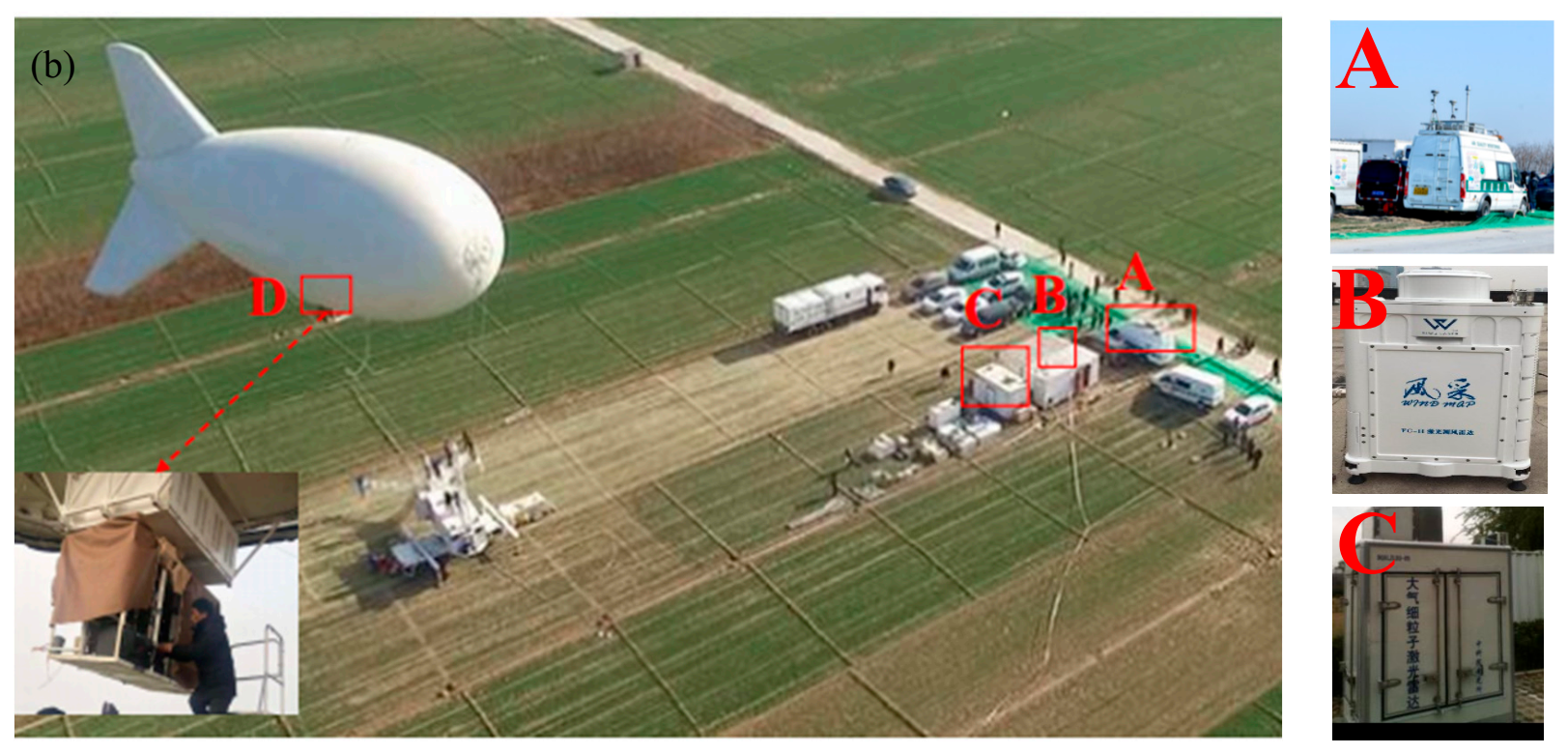
The shaded symbols in Figure 2a,b represent the extinction coefficients detected by the ground-based aerosol lidar. The pink line in Figure 2a represents the tethered balloon observation height, and the vector arrows in Figure 2b represent the horizontal wind vectors detected by the Doppler wind lidar. In this paper, the PBL heights were estimated by the wavelet transform method based on extinction coefficients [43,44]. It is worth noting that the PBL heights extracted by the extinction coefficients reflect the accumulation depth of aerosols in the atmosphere. In this paper, the vertical PBL structure was identified from the potential temperature profiles according to the top of the mixing layer, the top of the inversion layer and the top of the RL in combination with the relative humidity profiles. The vertical profiles at 20:00 on 19 December and 08:00 on 20 December were from radiosonde station 54511, while the other profiles were from the tethered balloon. The specific identification method is described in detail in Section 3.2.
As illustrated in Figure 2a, the PBL heights calculated by the ground-based aerosol lidar corresponded to different temperature stratification heights at different phases during the PBL evolution process. The lidar-calculated PBL heights varied mainly along the edge region, where the variation in the extinction coefficient is obvious. Compared with the temperature profiles, the lidar-determined PBL heights matched well with the top of the mixing layer during the daytime because the vertical diffusion heights reached by the pollutants in the strong mixing layer usually displayed dramatic changes in the extinction coefficients. However, the NBL heights approached closer to the RL top, especially before midnight, thus resulting in the relatively higher NBL heights determined by the aerosol lidar [29]. This phenomenon occurred because the RL serves as a storage mechanism for some pollutants and can affect the PBL heights calculated by lidar based on pollutants. The spatiotemporal distribution of extinction coefficients from 10:00 on 19 December to 14:00 on 19 December 2018, shows that larger extinction coefficient values were concentrated below 1000 m. After 14:00 on 19 December, pollutants accumulated gradually, and the extinction coefficients below 500 m increased distinctly, with the maximum value exceeding 1.5 km−1, revealing the existence of a thick aerosol layer. This thick aerosol layer led to a significant increase in the ground-level concentration of PM2.5, and NOχ (=NO+NO2) dominated among the gaseous precursors (shown in Figure 3a). Nitrogen oxides are important acidic gases that originate mainly from the combustion of carbon and fuel oil; the oxidant level in the atmosphere is usually measured by the total concentration of O3+ NO2 [45,46]. The high level of oxidants indicated that the concentration of secondary pollutants in the vicinity was relatively serious [47]. The nocturnal concentration of O3+ NO2 in Wangdu County was relatively high, which was conducive to the formation of secondary pollutant particulates.
The pollutants in the lower layer accumulated until approximately 04:00 on 20 December, after which the aerosol concentration decreased slightly within 250–500 m, demonstrating a multi-layer aerosol structure. The NBL height was relatively close to the top of the surface inversion layer after 04:00 on 20 December until the mixing layer was fully established. A proportion of pollutants remained in the RL at heights above 500 m. As illustrated in Figure 2a, some of the pollutants within this layer demonstrated evident sedimentation at approximately 06:00 on 20 December. With the gradual establishment of the mixing layer the next day, these trapped pollutants were fully integrated into the mixing layer, thus affecting the local air quality [19]. Moreover, the pollutants below 300 m did not diffuse easily due to the establishment of a deep stable inversion layer during the nighttime, and these pollutants maintained a high concentration; thus, the pollutants monitored near the surface did not disperse immediately.
Until 12:00 on 20 December, with the strong vertical mixing in the CBL, the momentum of the upper layer was easily transmitted downward to the ground; therefore, the ground wind speed exhibited a slight increasing trend. With the increase in the wind speed and the strong mixing diffusion in the PBL, the PM2.5, NOχ and SO2 near the surface could be transported upward into the PBL, and as a result, their surface concentrations were reduced [18]. In addition, the decrease in NOχ may also have been due to the increased consumption of precursor NOχ after sunrise. However, the ground-level ozone concentration increased to approximately 20 ppb, which is consistent with observations in Houston [19].
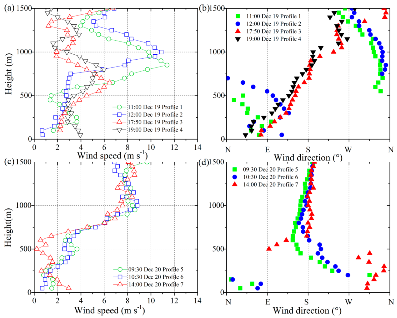
The vertical distributions of pollutants and winds were closely related, as shown in Figure 2b. The Doppler wind lidar observations show that an easterly wind dominated the lower layer, while a northwesterly wind dominated the upper layer from approximately 10:00 to 15:00 on 19 December. Moreover, the height at which the wind direction from the ground changed to a northwesterly wind corresponded to the edge region characterized by a large gradient of extinction coefficients. During the period from 15:00 to 21:00 on 19 December, the easterly wind still prevailed in the lower level, but the northwesterly wind in the upper level changed gradually into a westerly wind. At this time, the wind speed within the whole layer (including the RL) gradually decreased, which was conducive to the accumulation of pollutants. The extinction coefficients observed by the aerosol lidar and the ground-level pollutant concentrations gradually increased during this period. Subsequently, the PBL was dominated by southwesterly or southerly winds.
3.2. Identification of the Vertical Structure of Nocturnal Boundary Layer Observed by the Tethered Balloon
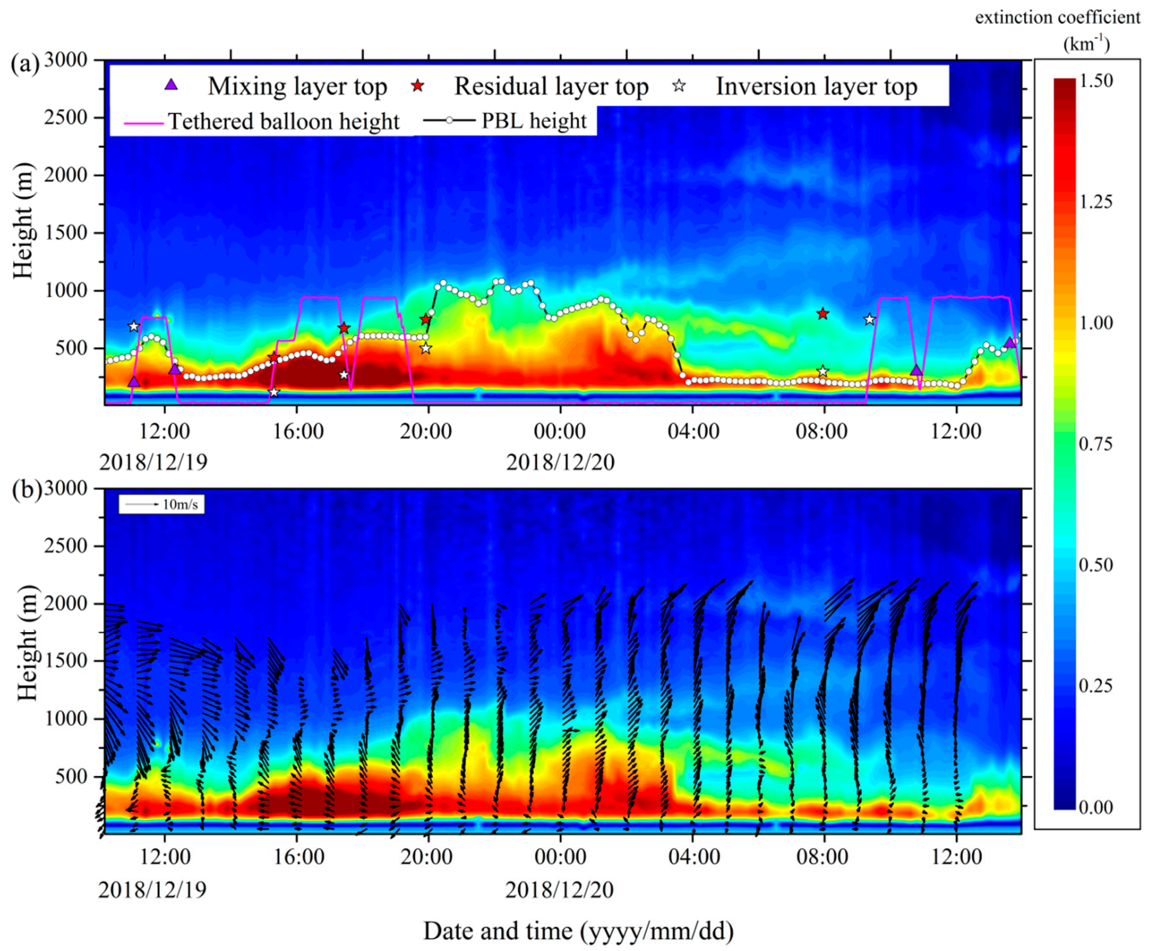
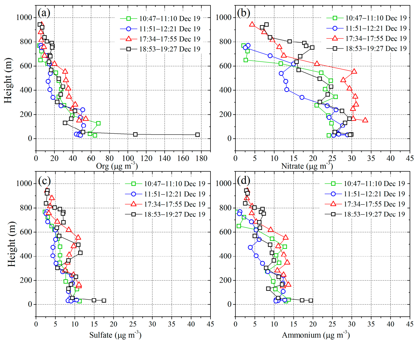
According to the tethered balloon observations at the different stages of PBL development, the RL was identified by the vertical profiles of the potential temperature. The vertical distributions of pollutants are closely related to the stratification of the atmospheric temperature [48]. In addition, atmospheric pollutant compounds are very complex, among which secondary aerosols constitute the main component of fine particles suspended in the atmosphere during periods of serious pollution, accounting for up to 70% [49]. Secondary inorganic aerosol particles, namely, sulfates, nitrates and ammonium salts, as well as Org compounds, were analyzed in this paper. The potential temperature below 200 m during 10:47–11:10 on 19 December (Figure 4) changed slightly with the height, generally presenting the characteristics of the mixing layer [50]; furthermore, the relative humidity at 200 m exhibited a significant negative gradient. The capping inversion layer thickness above the mixing layer was nearly 400 m, and the capping inversion intensity reached nearly 0.016 K m−1. As a result, considerable concentrations of pollutants remained trapped in the capping inversion layer (Figure 2). This capping inversion layer appeared during daytime above the mixed layer. The pollutants were concentrated mainly below 600 m. Figure 5 shows that nitrates (23.9 ± 1.5 μg m−3) dominated the secondary inorganic aerosols, followed by ammonium (11.0 ± 1.7 μg m−3) and sulfate (7.8 ± 1.9 μg m−3). The vertical distributions of nitrates and ammonium salts were similar, indicating that nitrate existed mainly in the form of ammonium nitrate at this time [51]. Org compounds were more susceptible to the surface pollution sources, and the Org concentration at 150 m reached 70 μg m−3.
According to the vertical temperature profile during 11:51–12:21 on 19 December, the near-surface temperature increased remarkably because of the positive net radiation budget [5]. Combined with the relative humidity profile, the mixing layer height was approximately 311 m at this time (as shown in Figure 4). All vertical profiles of the analyzed pollutants (shown in Figure 5) illustrate that the concentrations dropped off significantly above 250 m, and the pollutants were more affected by the influence of the mixing layer at this time. The concentration of Org compounds near the ground decreased by approximately 17 μg m−3 as a result of the development of the mixing layer.
The SBL gradually developed after sunset during the period of 17:34–17:55 on 19 December (Figure 4). At this time, the cooling effect from the ground resulted in the formation of a surface inversion layer, and the top of this layer was located at approximately 270 m. The potential temperature remained essentially unchanged in the range of 270–675 m and exhibited some daytime mixing layer features, indicating the formation of a typical RL [40], and the RL top was at a height of approximately 675 m. Just after sunset, the RL was relatively thick with a depth of approximately 400 m, and the relative humidity decreased significantly at the top of the RL. The observation results from the tethered balloon directly reveal that a considerable proportion of pollutants remained in the RL just after sunset (Figure 4). The nitrate concentration in the RL was very high, comparable to that of the Org compounds, sustained at approximately 30 μg m−3. This phenomenon was partly due to the increased formation of nitrates in the daytime under solar conditions [52]. Ground monitors also demonstrated that emissions of the nitrate precursor NOχ increased at this time, providing the basic conditions for nitrate formation (as illustrated in Figure 3). The vertical distributions of ammonium salt and nitrate were similar with uniform mixing below 600 m. The vertical sulfate distribution clearly reflected the storage capacity of the RL and the influence of the surface emission sources. According to the vertical distributions of these pollutants, the daytime mixing layer depth over Wangdu County was inferred to be approximately 600 m in the winter. Various emitted pollutants were well-mixed in the mixing layer. With the transition from a PBL to an SBL after sunset, the RL serves as a storage mechanism for some pollutants, and the influence of these pollutants on the local air quality through vertical mixing on the following day cannot be ignored.
The profile at 18:53–19:27 on 19 December demonstrated a typical SBL structure due to the continuous cooling caused by the negative radiation budget after sunset. The rising demand for electricity and winter heating factors after sunset elevated the combustion of gas, straw and coal [53]; consequently, the near-surface concentration of Org compounds increased substantially (Figure 5), reaching a maximum of 180 μg m−3. The concentration of sulfates also increased significantly in the lower layer. In contrast, the pollutant concentrations near 750 m in the RL increased only slightly, which may have been the result of the advection process with a relatively high pollutant concentration or of the chemical reaction process within the RL.
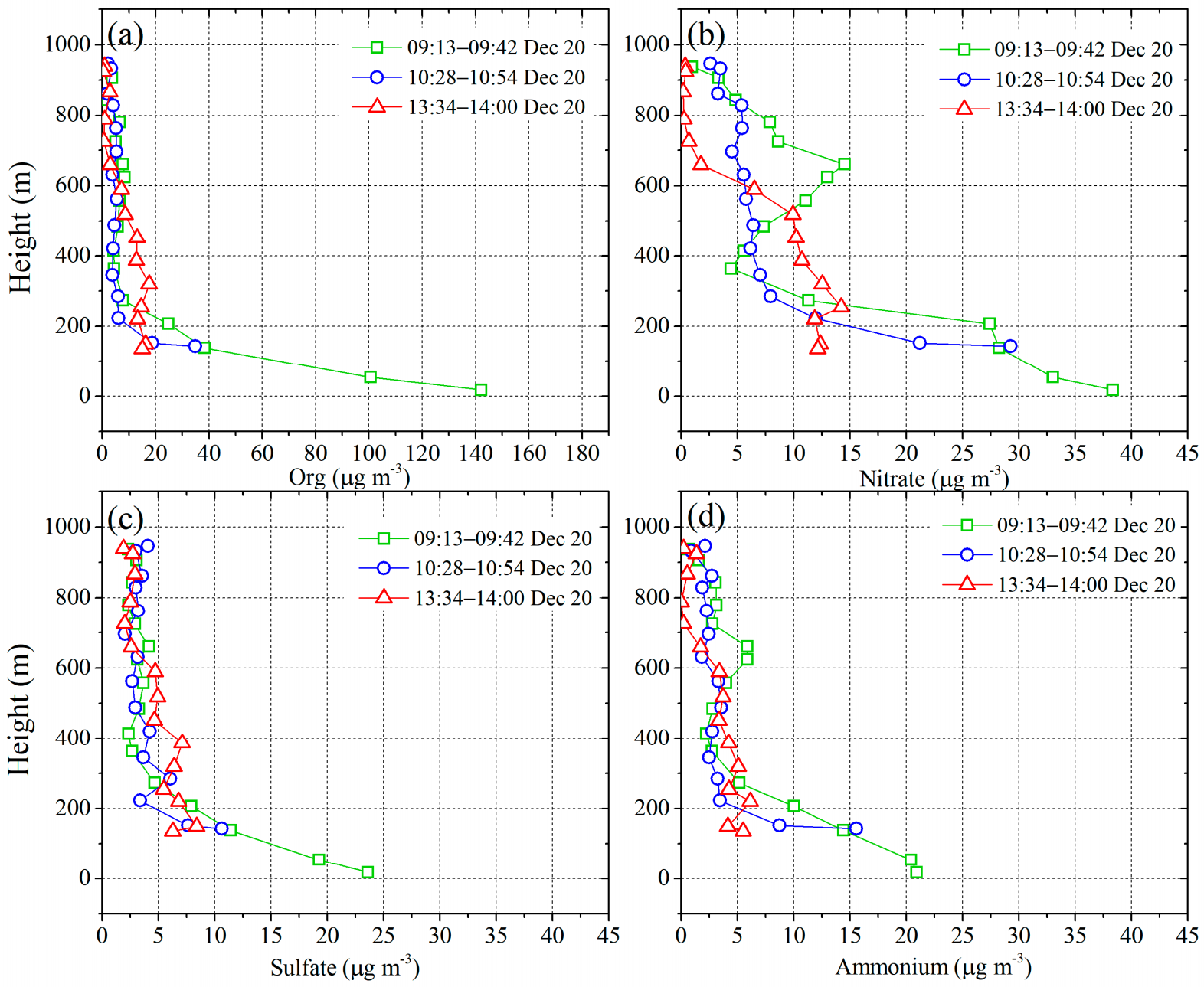
The vertical profile of the potential temperature at 09:13–09:42 on 20 December still reflected a typical SBL (Figure 5). However, the potential temperature gradient at the top of the SBL had clearly changed [54,55]. At this time, the SBL height, i.e., the top of the surface inversion layer, formed by the surface cooling effect was approximately 700 m. The inversion intensity was also high and basically displayed a linear decreasing trend [54]. From 700 m to 950 m, the potential temperature remained nearly unchanged with the height, thereby reflecting an RL structure. After sunrise, the vertical profiles of the pollutants (shown in Figure 6) were characterized by the highest concentrations near the ground; this phenomenon was related to the poor diffusion conditions in the nocturnal SBL, and was also affected by the blocking effect of the inversion layer. Another notable feature was the storage of pollutants in the RL [18]. The concentration of nitrates in the RL was very high, close to 10 μg m−3. Subsequently, the potential temperature profile at 10:28–10:54 on 20 December (Figure 4) illustrated that the surface inversion layer dissipated as a consequence of surface warming; in addition, the top of the mixing layer was situated at approximately 300 m until 13:34, when the top of the mixing layer rose to 540 m.
As shown in Figure 7c,d, except for the decrease in the wind speed in the range of 250–750 m at 14:00, the vertical profiles of the horizontal wind speed from three tethered balloon observation periods on 20 December 2018, were nearly identical at 09:30, 10:30 and 14:00; in particular, at the relatively low level of 750 m, the wind speed was basically less than 4 m s−1, and the wind direction around 700 m showed little change. Therefore, during this period, the vertical distribution of pollutants caused by advection below 750 m can be neglected to some extent and can be considered the result of the evolution of either the vertical PBL structure or the local emission sources.
Moreover, strong daytime mixing entrained the pollutants in the RL downward, decreasing the pollutant concentrations in the RL. The nitrate concentration in the RL near 700 m decreased from approximately 12 μg m−3 to 5 μg m−3 (Figure 6), and the nitrate concentration at this height further decreased to about 2 μg m−3 until 13:34. The case analyzed here shows that the mixing down of nitrate from the RL can contribute about 37% to the nitrate in the mixing layer. The relatively higher contribution from the photochemical production to nitrate was observed in the afternoon, and the maximum nitrate concentration in the developing mixing layer exceeded 12 μg m−3 at 13:34 20 December. The vertical distribution of ammonium salt was similar to that of nitrate, although the concentration of the former was slightly lower than that of the latter. Pollutants emitted near the surface were also capable of diffusing upward under vertical turbulent mixing, and thus, the pollutant concentrations monitored on the ground exhibited a decreasing trend.
3.3. The Correlation between the Richardson Number and the Vertical Distribution of PM2.5
The vertical diffusion and mixing of pollutants in the PBL are closely related to turbulence; accordingly, we discussed the relationship between the vertical profile of PM2.5 and atmospheric turbulence fluctuations by calculating the bulk Richardson number (Rb). In this paper, based on the vertical temperature profile measured by the tethered balloon and the wind profiles observed by the Doppler wind lidar, the Rb was calculated by the difference method [5]. The specific formula is as follows:
where θ, U and z represent the potential temperature, horizontal wind speed, and height above the ground, respectively. The Rb is a dimensionless number that measures whether atmospheric turbulence can develop. When Rb < 0, the buoyancy term is positive; when Rb > 0, negative buoyancy inhibits the generation of turbulence; and when Rb > 1, turbulence activities can be completely suppressed [56]. As molecular viscous dissipation cannot be neglected, the Rb threshold is less than 1 when turbulence is completely inhibited. Although the critical Rb varies between flows or may not exist at all [57,58], a threshold value of 0.25 is taken as a reference.
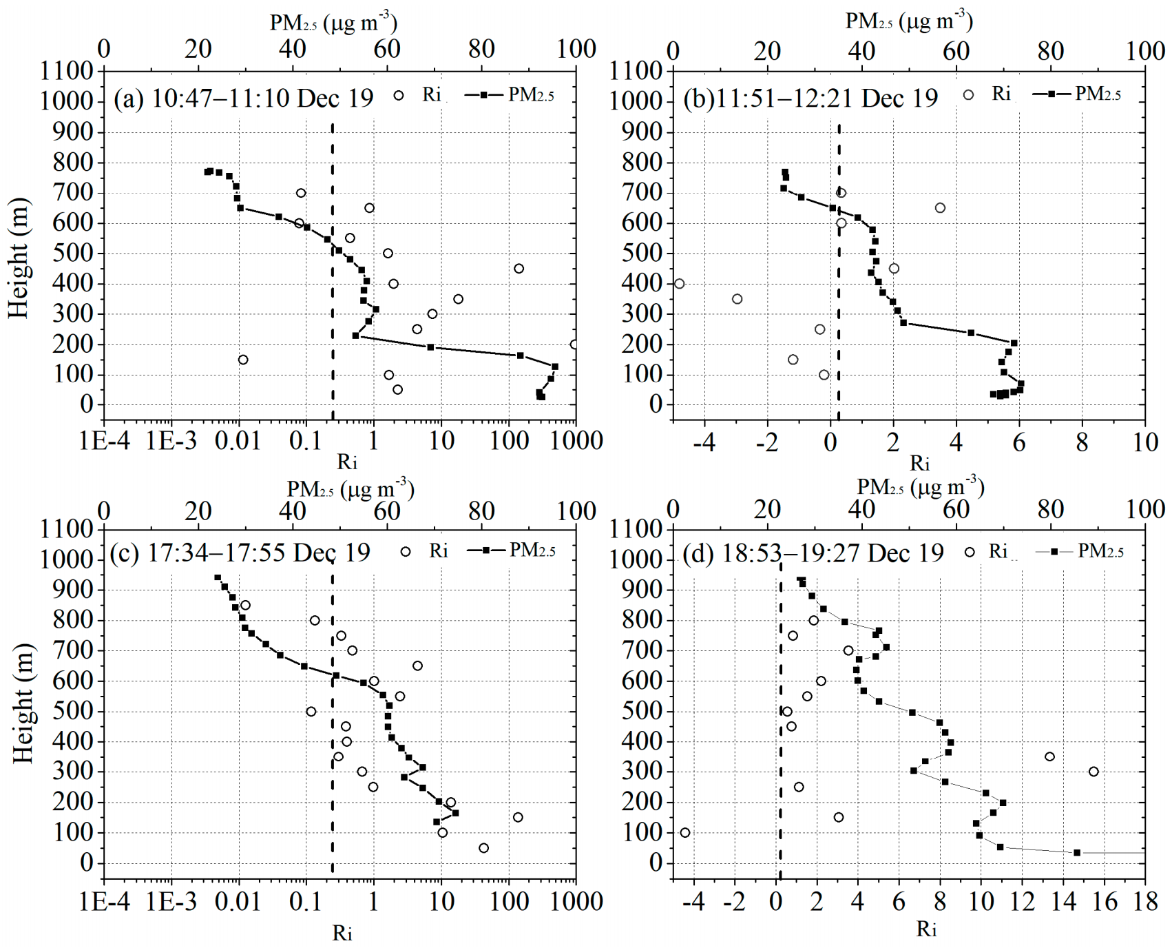
The profile at 10:47–11:10 on 19 December (Figure 8a) indicates that particles below 200 m with an Rb less than the threshold value of 0.25 were uniformly distributed during the early development of the mixing layer. In the capping inversion layer from 200 m to 600 m, the Rb exceeded the threshold value, and thus, the development of turbulent activity was greatly inhibited. The PM2.5 concentration was close to 60 μg m−3 in this layer and gradually decreased.
Subsequently, turbulent activity developed strongly with the continuously increasing solar radiation received by the surface; the profile at 11:51–12:21 on 19 December (Figure 8b) suggests that the atmospheric layer depth with an Rb less than 0.25 rose to 400 m. Near-surface PM2.5 continued to mix and diffuse vertically, and the concentration below 200 m decreased. The profile during 17:34–17:55 on 19 December (Figure 8c) shows that the Rb in the lower SBL was basically higher than 0.25, whereas the Rb in the middle of the RL above 400 m was less than the threshold value, revealing the occurrence of some remaining turbulence in the RL just after sunset [59]. At this time, the PM2.5 concentration below the RL decreased slowly, but the concentration of PM2.5 dropped rapidly across the top of the RL (~600 m). As the SBL gradually developed, the thickness of the RL became compressed when the whole layer was stable at 18:53 (Figure 8d). The Rb within the SBL exceeded 0.25; additionally, due to the influences of many factors, such as the RL and ground emission sources, the PM2.5 concentration in the SBL demonstrated a significant multi-layer distribution.
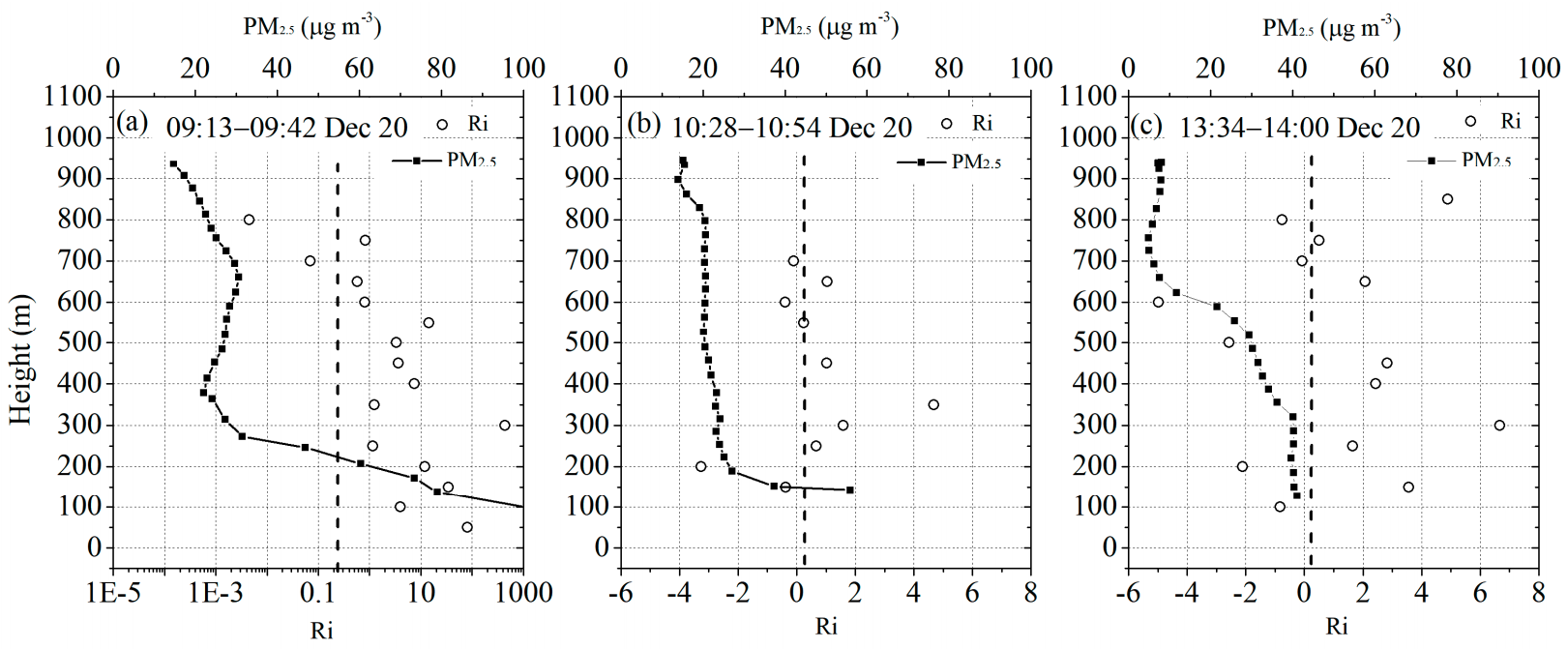
After the SBL developed overnight, as shown in Figure 9a, due to the suppressing effects of the surface inversion layer, the ground PM2.5 concentration was very high at 09:13–09:42 on 20 December (>100 μg m−3). The Rb was less than the threshold value within the RL at heights of 700–800 m, and there was a small increase in the concentration of particulates within this layer. This phenomenon may have been attributable to the locally supersaturated environment caused by turbulence after sunrise, which was conducive to the formation of new particles [33].
The concentration of nitrates was highest at this time (as shown in Figure 6). During 10:28–10:54 on 20 December (Figure 9b), the Rb was less than the threshold value below 200 m; however, the overall distribution of the PM2.5 concentration was somewhat uniform instead of being high near the surface. Assuming that the local emission intensity did not change considerably in a short time, the PM2.5 concentration near 700 m in the RL decreased from 30 μg m−3 in the early morning to 5 μg m−3 at 13:34–14:00 on 20 December (Figure 9c); in contrast, the PM2.5 payload in the mixing layer increased significantly, implying that the pollutants were entrained downward from the RL due to strong vertical mixing. Moreover, because the low-level horizontal wind changed little during the three observation periods (shown in Figure 7c,d), the advective transport of pollutants during this process is regarded as having a small impact.
4. Discussion
In this paper, based on a comprehensive and intensive observation campaign conducted in Wangdu County of the NCP, the evolution of NBL and its influences on the vertical distributions of pollutant particulates were analyzed.
The analysis results show that when the nocturnal SBL just formed after sunset, pollutant particulates remained suspended with high concentrations in the RL aloft. The extinction coefficient exceeded 1.5 km−1, and nitrates dominated among the secondary inorganic aerosol particles with a concentration close to 30 μg m−3 (17:34–17:55 on 19 December). Multi-layer pollutant structures appeared often because of the effects of the RL. After sunrise, the gradual establishment of the daytime mixing layer caused the pollutants stored within the previous nocturnal RL to be entrained downwards into the mixing layer. The PM2.5 concentration near 700 m in the RL on 19 December 2018, was approximately 30 μg m−3, and it dropped off to 5 μg m−3 at 13:34–14:40 on 19 December, decreasing by nearly 83% while the PM2.5 concentration in the mixing layer increased significantly. The mixing down of nitrate from the RL analyzed in this paper has contributed about 37% to the nitrate in the mixing layer. In addition, the ground-level PM2.5 concentrations after sunrise decreased partially because of the stronger vertical mixing in the daytime; the decreased NOχ was also due to additional consumption during the photochemical process, whereas the ozone concentration rose. In different stages of development of the PBL, the Rb exhibited corresponding characteristics. The Rb in the SBL basically exceeded its threshold value (0.25), and thus, turbulence was suppressed, while the Rb below the critical number in the RL was less than the critical value, indicating the generation of turbulence. The corresponding increment in the morning PM2.5 concentration may have been closely related to the turbulence within the RL. Moreover, the concentrations of ammonium salts and nitrates increased obviously within the RL, but Org compounds and sulfates did not change significantly. The estimated mixing layer depth over Wangdu County was approximately 600 m in winter. The PBL height calculated by aerosol lidar matched well with the top of the daytime mixing layer; however, the NBL height calculated by aerosol lidar was closer to the top of the RL because the surface inversion layer has not fully developed during this period. Due to the storage of pollutants in the RL, the NBL height estimated by the aerosol lidar reflecting the accumulation depth for pollutants often overestimated the nocturnal SBL height, especially prior to midnight. After midnight, the NBL height was more consistent with the top of the surface inversion layer.
Author Contributions
The work presented here was carried out with collaboration among all the authors. Conceptualization, Y.S. and F.H.; methodology, Y.S.; formal analysis, Y.S. and L.L.; data curation, G.F. and J.H. All authors carried out the experiments. All authors have read and agreed to the published version of the manuscript.
Funding
This article was founded by the National Key Research and Development Program of China.
Data Availability Statement
The data presented in this study are available on request from the corresponding author.
Acknowledgments
This work was supported by the National Key Research and Development Program of China (2017YFC0209605), the General Financial Grant from the China Postdoctoral Science Foundation (2020M670420), the Special Research Assistant Project and the National Natural Science Foundation of China (Grant 41975018).
Conflicts of Interest
The authors declare no conflict of interest.
References
- Quan, J.; Liu, Y.; Liu, Q.; Jia, X.; Li, X.; Gao, Y.; Ding, D.; Li, J.; Wang, Z. Anthropogenic pollution elevates the peak height of new particle formation from planetary boundary layer to lower free troposphere. Geophys. Res. Lett. 2017, 44, 7537–7543. [Google Scholar] [CrossRef]
- Chang, D.; Wang, Z.; Guo, J.; Li, T.; Liang, Y.; Kang, L.; Xia, M.; Wang, Y.; Yu, C.; Yun, H.; et al. Characterization of organic aerosols and their precursors in southern China during a severe haze episode in January 2017. Sci. Total Environ. 2019, 691, 101–111. [Google Scholar] [CrossRef] [PubMed]
- Li, L.; Lu, C.; Chan, P.W.; Zhang, X.; Yang, H.L.; Lan, Z.J.; Zhang, W.H.; Liu, Y.W.; Pan, L.; Zhang, L. Tower observed vertical distribution of PM2.5, O-3 and NOx in the Pearl River Delta. Atmos. Environ. 2020, 220, 117083. [Google Scholar] [CrossRef]
- Yoshino, A.; Takami, A.; Hara, K.; Nishita-Hara, C.; Hayashi, M.; Kaneyasu, N. Contribution of Local and Transboundary Air Pollution to the Urban Air Quality of Fukuoka, Japan. Atmosphere 2021, 12, 431. [Google Scholar] [CrossRef]
- Stull, R.B. An Introduction to Boundary Layer Meteorology; Kluwer Academic Publishers: Dordrecht, The Netherlands, 1988. [Google Scholar]
- Glickman, T.S.; Zenk, W. Glossary of Meteorology; American Meteorological Society: Boston, MA, USA, 2000. [Google Scholar]
- Blay-Carreras, E.; Pino, D.; Arellano, J.V.-G.d.; Boer, A.V.d.; Coster, O.d.; Darbieu, C.; Hartogensis, O.K.; Lohou, F.; Lothon, M.; Pietersen, H.P. Role of the residual layer and large-scale subsidence on the development and evolution of the convective boundary layer. Atmos. Chem. Phys. 2014, 14, 4515–4530. [Google Scholar] [CrossRef] [Green Version]
- Salmond, J.A.; McKendry, I.G. A review of turbulence in the very stable nocturnal boundary layer and its implications for air quality. Prog. Phys. Geogr. Earth Environ. 2005, 29, 171–188. [Google Scholar] [CrossRef] [Green Version]
- Jansen, R.C.; Shi, Y.; Chen, J.; Hu, Y.; Xu, C.; Hong, S.; Li, J.; Zhang, M. Using Hourly Measurements to Explore the Role of Secondary Inorganic Aerosol in PM 2.5 during Haze and Fog in Hangzhou, China. Adv. Atmos. Sci. 2014, 31, 1427–1434. [Google Scholar] [CrossRef]
- Wu, P.; Ding, Y.H.; Liu, Y.J. Atmospheric circulation and dynamic mechanism for persistent haze events in the Beijing–Tianjin–Hebei region. Adv. Atmos. Sci. 2017, 34, 429–440. [Google Scholar] [CrossRef] [Green Version]
- Sun, J.; Wang, Y.; Wu, F.; Tang, G.; Wang, L.; Wang, Y.; Yang, Y. Vertical characteristics of VOCs in the lower troposphere over the North China Plain during pollution periods. Environ. Pollut. 2017, 236, 907–915. [Google Scholar] [CrossRef]
- Zhang, Q.; Ma, Q.; Zhao, B.; Liu, X.; Wang, Y.; Jia, B.; Zhang, X. Winter haze over North China Plain from 2009 to 2016: Influence of emission and meteorology. Environ. Pollut. 2018, 242, 1308–1318. [Google Scholar] [CrossRef]
- Shi, Y.; Hu, F.; Fan, G.; Zhang, Z. Multiple technical observations of the atmospheric boundary layer structure of a red-alert haze episode in Beijing. Atmos. Meas. Tech. 2019, 12, 4887–4901. [Google Scholar] [CrossRef] [Green Version]
- Hu, X.-M.; Klein, P.M.; Xue, M.; Zhang, F.; Doughty, D.C.; Forkel, R.; Joseph, E.; Fuentes, J.D. Impact of the vertical mixing induced by low-level jets on boundary layer ozone concentration. Atmos. Environ. 2013, 70, 123–130. [Google Scholar] [CrossRef] [Green Version]
- Madonna, F.; Summa, D.; Girolamo, P.D.; Marra, F.; Wang, Y.; Rosoldi, M. Assessment of Trends and Uncertainties in the Atmospheric Boundary Layer Height Estimated using Radiosounding Observations over Europe. Atmosphere 2021, 12, 301. [Google Scholar] [CrossRef]
- Vivone, G.; D’Amico, G.; Summa, D.; Lolli, S.; Amodeo, A.; Bortoli, D.; Pappalardo, G. Atmospheric Boundary Layer height estimation from aerosol lidar: A new approach based on morphological image processing techniques. Atmos. Chem. Phys. Discuss. 2021, 21, 4249–4265. [Google Scholar] [CrossRef]
- Ma, J.Z.; Wang, W.; Chen, Y.; Liu, H.J.; Yan, P.; Ding, G.A.; Wang, M.L.; Sun, J.; Lelieveld, J. The IPAC-NC field campaign: A pollution and oxidization pool in the lower atmosphere over Huabei, China. Atmos. Chem. Phys. 2012, 12, 3883–3908. [Google Scholar] [CrossRef] [Green Version]
- Zhang, J.; Rao, S.T. The Role of Vertical Mixing in the Temporal Evolution of Ground-Level Ozone Concentrations. J. Appl. Meteorol. 1999, 38, 1674–1691. [Google Scholar] [CrossRef] [Green Version]
- Morris, G.A.; Ford, B.; Rappenglück, B.; Thompson, A.M.; Mefferd, A.; Ngan, F.; Lefer, B. An evaluation of the interaction of morning residual layer and afternoon mixed layer ozone in Houston using ozonesonde data. Atmos. Environ. 2010, 44, 4024–4034. [Google Scholar] [CrossRef]
- Emeis, S.; Schäfer, K. Remote Sensing Methods to Investigate Boundary-layer Structures relevant to Air Pollution in Cities. Bound. Layer Meteorol. 2006, 121, 377–385. [Google Scholar] [CrossRef]
- Blary, F.; Ziad, A.; Borgnino, J.; Fanteï-Caujolle, Y.; Aristidi, E.; Lanteri, H. Monitoring atmospheric turbulence profiles with high vertical resolution using PML/PBL instrument. In Proceedings of the SPIE Astronomical Telescopes + Instrumentation, Montréal, QC, Canada, 22–27 June 2014. [Google Scholar]
- Luo, T.; Yuan, R.; Wang, Z. Lidar-based remote sensing of atmospheric boundary layer height over land and ocean. Atmos. Meas. Tech. 2013, 7, 173–182. [Google Scholar] [CrossRef] [Green Version]
- Banakh, V.; Smalikho, I.; Falits, A. Estimation of the height of the turbulent mixing layer from data of Doppler lidar measurements using conical scanning by a probe beam. Atmos. Meas. Tech. 2021, 14, 1511–1524. [Google Scholar] [CrossRef]
- Shikhovtsev, A.Y.; Kiselev, A.V.; Kovadlo, P.G.; Kolobov, D.Y.; Lukin, V.P.; Tomin, V.E. Method for Estimating the Altitudes of Atmospheric Layers with Strong Turbulence. Atmos. Ocean. Opt. 2020, 33, 295–301. [Google Scholar] [CrossRef]
- Potekaev, A.; Shamanaeva, L.; Kulagina, V. Spatiotemporal Dynamics of the Kinetic Energy in the Atmospheric Boundary Layer from Minisodar Measurements. Atmosphere 2021, 12, 421. [Google Scholar] [CrossRef]
- Kovadlo, P.; Shikhovtsev, A.; Kopylov, E.; Kiselev, A.; Russkikh, I. Study of the Optical Atmospheric Distortions using Wavefront Sensor Data. Russ. Phys. J. 2021, 63, 1952–1958. [Google Scholar] [CrossRef]
- Seibert, P.; Beyrich, F.; Gryning, S.-E.; Joffre, S.; Rasmussen, A.; Tercier, P. Review and intercomparison of operational methods for the determination of the mixing height. Atmos. Environ. 2000, 34, 1001–1027. [Google Scholar] [CrossRef]
- Wang, Z.; Cao, X.; Zhang, L.; Notholt, J.; Zhou, B.; Liu, R.; Zhang, B. Lidar measurement of planetary boundary layer height and comparison with microwave profiling radiometer observation. Atmos. Meas. Tech. 2012, 5, 1965–1972. [Google Scholar] [CrossRef] [Green Version]
- Quan, J.; Gao, Y.; Zhang, Q.; Tie, X.; Cao, J.; Han, S.; Meng, J.; Chen, P.; Zhao, D. Evolution of planetary boundary layer under different weather conditions, and its impact on aerosol concentrations. Particuology 2013, 11, 34–40. [Google Scholar] [CrossRef]
- Shi, Y.; Hu, F.; Xiao, Z.; Fan, G.; Zhang, Z. Comparison of four different types of planetary boundary layer heights during a haze episode in Beijing. Sci. Total Environ. 2020, 711, 134928. [Google Scholar] [CrossRef] [PubMed]
- Santacesaria, V.; Marenco, F.; Balis, D.; Papayannis, A.; Zerefos, C. Lidar observations of the Planetary Boundary Layer above the city of Thessaloniki, Greece. Nuovo Cimento 1998, 21, 585–596. [Google Scholar]
- Lei, H.; Wuebbles, D.J. Chemical competition in nitrate and sulfate formations and its effect on air quality. Atmos. Environ. 2013, 80, 472–477. [Google Scholar] [CrossRef]
- Wehner, B.; Siebert, H.; Ansmann, A.; Ditas, F.; Seifert, P.; Stratmann, F.; Wiedensohler, A.; Apituley, A.; Shaw, R.A.; Manninen, H.E.; et al. Observations of turbulence-induced new particle formation in the residual layer. Atmos. Chem. Phys. 2010, 10, 4319–4330. [Google Scholar] [CrossRef] [Green Version]
- Siebert, H.; Wehner, B.; Hellmuth, O.; Stratmann, F.; Boy, M.; Kulmala, M. New-particle formation in connection with a nocturnal low-level jet: Observations and modeling results. Geophys. Res. Lett. 2007, 34. [Google Scholar] [CrossRef]
- Sangiorgi, G.; Ferrero, L.; Perrone, M.G.; Bolzacchini, E.; Duane, M.; Larsen, B.R. Vertical distribution of hydrocarbons in the low troposphere below and above the mixing height: Tethered balloon measurements in Milan, Italy. Environ. Pollut. 2011, 159, 3545–3552. [Google Scholar] [CrossRef]
- Zhang, K.; Zhou, L.; Fu, Q.; Yan, L.; Bian, Q.; Wang, D.; Xiu, G. Vertical distribution of ozone over Shanghai during late spring: A balloon-borne observation. Atmos. Environ. 2019, 208, 48–60. [Google Scholar] [CrossRef]
- Chan, C.Y.; Xu, X.D.; Li, Y.S.; Wong, K.H.; Ding, G.A.; Chan, L.Y.; Cheng, X.H. Characteristics of vertical profiles and sources of PM2.5, PM10 and carbonaceous species in Beijing. Atmos. Environ. 2005, 39, 5113–5124. [Google Scholar] [CrossRef]
- Ting, M.; Yue-si, W.; Jie, J.; Fang-kun, W.; Mingxing, W. The vertical distributions of VOCs in the atmosphere of Beijing in autumn. Sci. Total Environ. 2008, 390, 97–108. [Google Scholar] [CrossRef]
- Sun, Y. Vertical structures of physical and chemical properties of urban boundary layer and formation mechanisms of atmospheric pollution. Chin. Sci. Bull. 2018, 63, 1374–1389. [Google Scholar] [CrossRef] [Green Version]
- Neu, U.; Künzle, T.; Wanner, H. On the relation between ozone storage in the residual layer and daily variation in near-surface ozone concentration: A case study. Bound. Layer Meteorol. 1994, 69, 221–247. [Google Scholar] [CrossRef]
- Rappenglück, B.; Perna, R.; Zhong, S.; Morris, G.A. An analysis of the vertical structure of the atmosphere and the upper-level meteorology and their impact on surface ozone levels in Houston, Texas. J. Geophys. Res. 2008, 113. [Google Scholar] [CrossRef]
- Sun, H.; Shi, Y.; Liu, L.; Ding, W.; Zhang, Z.; Hu, F. Impacts of Atmospheric Boundary Layer Vertical Structure on Haze Pollution Observed by Tethered Balloon and Lidar. J. Meteorol. Res. 2021, 35, 209–223. [Google Scholar] [CrossRef]
- Cohn, S.A.; Angevine, W.M. Boundary Layer Height and Entrainment Zone Thickness Measured by Lidars and Wind-Profiling Radars. J. Appl. Meteorol. 2000, 39, 1233–1247. [Google Scholar] [CrossRef]
- Brooks, I.M. Finding Boundary Layer Top: Application of a Wavelet Covariance Transform to Lidar Backscatter Profiles. J. Atmos. Ocean. Technol. 2003, 20, 1092–1105. [Google Scholar] [CrossRef] [Green Version]
- Stephens, S.; Madronich, S.; Wu, F.; Olson, J.B.; Ramos, R.; Retama, A.; Muñoz, R. Weekly patterns of México City’s surface concentrations of CO, NOx, PM10 and O3 during 1986–2007. Atmos. Chem. Phys. 2008, 8, 5313–5325. [Google Scholar] [CrossRef] [Green Version]
- Yang, C.; Li, H.; Chen, R.; Xu, W.; Wang, C.; Tse, L.A.; Zhao, Z.; Kan, H. Combined atmospheric oxidant capacity and increased levels of exhaled nitric oxide. Environ. Res. Lett. 2016, 11, 74014. [Google Scholar] [CrossRef]
- Hallquist, M.; Wenger, J.C.; Baltensperger, U.; Rudich, Y.; Simpson, D.; Claeys, M.; Dommen, J.; Donahue, N.M.; George, C.; Goldstein, A.H.; et al. The formation, properties and impact of secondary organic aerosol: Current and emerging issues. Atmos. Chem. Phys. 2009, 9, 5155–5236. [Google Scholar] [CrossRef] [Green Version]
- Largeron, Y.; Staquet, C. Persistent inversion dynamics and wintertime PM10 air pollution in Alpine valleys. Atmos. Environ. 2016, 135, 92–108. [Google Scholar] [CrossRef]
- Volkamer, R.; Jimenez, J.L.; Martini, F.S.; Dzepina, K.; Zhang, Q.; Salcedo, D.; Molina, L.T.; Worsnop, D.R.; Molina, M.J. Secondary organic aerosol formation from anthropogenic air pollution: Rapid and higher than expected. Geophys. Res. Lett. 2006, 33. [Google Scholar] [CrossRef] [Green Version]
- Day, B.M.; Rappenglück, B.; Clements, C.B.; Tucker, S.C.; Brewer, W.A. Nocturnal boundary layer characteristics and land breeze development in Houston, Texas during TexAQS II. Atmos. Environ. 2010, 44, 4014–4023. [Google Scholar] [CrossRef]
- Nowak, J.B.; Neuman, J.A.; Bahreini, R.; Brock, C.A.; Middlebrook, A.M.; Wollny, A.G.; Holloway, J.S.; Peischl, J.; Ryerson, T.B.; Fehsenfeld, F.C. Airborne observations of ammonia and ammonium nitrate formation over Houston, Texas. J. Geophys. Res. Space Phys. 2010, 115. [Google Scholar] [CrossRef] [Green Version]
- Richards, L.W. Comments on the oxidation of NO2 to nitrate—Day and night. Atmos. Environ. 1983, 17, 397–402. [Google Scholar] [CrossRef]
- Duan, F.; Liu, X.; Yu, T.; Cachier, H. Identification and estimate of biomass burning contribution to the urban aerosol organic carbon concentrations in Beijing. Atmos. Environ. 2004, 38, 1275–1282. [Google Scholar] [CrossRef]
- Carlson, M.A.; Stull, R.B. Subsidence in the Nocturnal Boundary Layer. J. Clim. Appl. Meteorol. 1986, 25, 1088–1099. [Google Scholar] [CrossRef] [Green Version]
- Summa, D.; Girolamo, P.D.; Stelitano, D.; Cacciani, M. Characterization of the planetary boundary layer height and structure by Raman lidar: Comparison of different approaches. Atmos. Meas. Tech. 2013, 6, 3515–3525. [Google Scholar] [CrossRef] [Green Version]
- Tjernström, M.; Balsley, B.B.; Svensson, G.; Nappo, C.J. The Effects of Critical Layers on Residual Layer Turbulence. J. Atmos. Sci. 2009, 66, 468–480. [Google Scholar] [CrossRef]
- Zilitinkevich, S.S.; Elperin, T.; Kleeorin, N.; Rogachevskii, I. Energy- and flux-budget (EFB) turbulence closure model for stably stratified flows. Bound. Layer Meteorol. 2006, 125, 167–191. [Google Scholar] [CrossRef] [Green Version]
- Mahrt, L. Variability and Maintenance of Turbulence in the Very Stable Boundary Layer. Bound. Layer Meteorol. 2010, 135, 1–18. [Google Scholar] [CrossRef] [Green Version]
- Muschinski, A.; Frehlich, R.G.; Balsley, B.B. Small-scale and large-scale intermittency in the nocturnal boundary layer and the residual layer. J. Fluid Mech. 2004, 515, 319–351. [Google Scholar] [CrossRef] [Green Version]
Figure 1.
(a) Map of the local topography of the North China Plain; the red circle represents the sampling site in Wangdu County. The map was retrieved from Google Maps©. (b) Large tethered balloon detection platform and ground-based observation instruments utilized during the observation period in Wangdu County. A: Atmospheric environment monitoring vehicle; B: Doppler wind lidar; C: Ground-based aerosol lidar square; D: Tethered balloon observation platform.


Figure 2.
(a) Spatiotemporal evolution of extinction coefficients observed by ground-based aerosol lidar. The pink line is the observation height of the tethered balloon, the white circular line is the PBL calculated by aerosol lidar using the wavelet transform method, and the boundary layer heights corresponded to different temperature stratification heights. (b) The shaded symbols represent the extinction coefficients determined by aerosol lidar, and the black vector arrows represent the horizontal wind vectors detected by Doppler wind lidar. The observation times of both graphs range from 10:00 on 19 December 2018, to 14:00 on 20 December 2018.

Figure 3.
(a) Time series variations of the PM2.5, SO2, O3 and NOχ concentrations observed on the ground; the units for PM2.5 are micrometers per cubic meter, while the units for SO2, O3 and NOχ are ppb; (b) ground wind speed and wind direction, where the units are meters per second and degrees, respectively. All variables were observed by a mobile monitoring vehicle. The three stages in this paper are classified as, Stage 1, 10:00 to 17:00 on 19 December 2018, the evolution from a CBL to an NBL with an emerging RL; Stage 2, from 17:00 on 19 December 2018 to 07:30 on 20 December 2018, after sunset, when the SBL gradually develops until sunrise the following day, leaving a morning RL; and Stage 3, from 07:30 to 14:00 on 20 December 2018, the daytime CBL gradually matures after sunrise while the morning RL disappears.

Figure 4.
(a) Vertical profiles of the potential temperature and (b) relative humidity detected by the large tethered balloon on 19 December and 20 December 2018. Taking the profile during 09:13–09:42 on 20 December as an example, the estimated base of the RL was at approximately 700 m, and the potential temperature remained constant above 700 m.

Figure 5.
Vertical profiles of the concentrations of Org compounds (a), nitrates (b), sulfates (c) and ammonium salts (d) observed by the large tethered balloon on 19 December 2018; the units for these pollutant particulates are micrometers per cubic meter.
Figure 5.
Vertical profiles of the concentrations of Org compounds (a), nitrates (b), sulfates (c) and ammonium salts (d) observed by the large tethered balloon on 19 December 2018; the units for these pollutant particulates are micrometers per cubic meter.

Figure 6.
Vertical profiles of the concentrations of Org compounds (a), nitrates (b), sulfates (c) and ammonium salts (d) observed by the large tethered balloon on 20 December 2018; the units for these pollutant particulates are micrometers per cubic meter.
Figure 6.
Vertical profiles of the concentrations of Org compounds (a), nitrates (b), sulfates (c) and ammonium salts (d) observed by the large tethered balloon on 20 December 2018; the units for these pollutant particulates are micrometers per cubic meter.

Figure 7.
Vertical profiles of the horizontal wind speed (a,c) and wind direction (b,d) for Profiles 1–7 during the tethered balloon observation period measured by Doppler wind lidar.
Figure 7.
Vertical profiles of the horizontal wind speed (a,c) and wind direction (b,d) for Profiles 1–7 during the tethered balloon observation period measured by Doppler wind lidar.

Figure 8.
Profiles of the Rb and PM2.5 concentration (micrometers per cubic meter) observed by the tethered balloon during the observation period on 19 December 2018.
Figure 8.
Profiles of the Rb and PM2.5 concentration (micrometers per cubic meter) observed by the tethered balloon during the observation period on 19 December 2018.

Figure 9.
Vertical profiles of the Rb and PM2.5 concentration (micrometers per cubic meter) observed by the tethered balloon during the observation period on 20 December 2018.
Figure 9.
Vertical profiles of the Rb and PM2.5 concentration (micrometers per cubic meter) observed by the tethered balloon during the observation period on 20 December 2018.


Table 1.
Altitude detection records and ascending times of the large tethered balloon.
| Detection | Profile 1 | Profile 2 | Profile 3 | Profile 4 | Profile 5 | Profile 6 | Profile 7 |
|---|---|---|---|---|---|---|---|
| Height | 250–772 m | 769–27 m | 246–942 m | 940–34 m | 17–937 m | 946–142 m | 940–149 m |
| Time | 10:47–11:10 | 11:51–12:21 | 17:34–17:55 | 18:53–19:27 | 09:13–09:42 | 10:28–10:54 | 13:34–14:00 |
| Date | 19 December | 19 December | 19 December | 19 December | 20 December | 20 December | 20 December |
Publisher’s Note: MDPI stays neutral with regard to jurisdictional claims in published maps and institutional affiliations. |
© 2021 by the authors. Licensee MDPI, Basel, Switzerland. This article is an open access article distributed under the terms and conditions of the Creative Commons Attribution (CC BY) license (https://creativecommons.org/licenses/by/4.0/).
Share and Cite
MDPI and ACS Style
Shi, Y.; Liu, L.; Hu, F.; Fan, G.; Huo, J. Nocturnal Boundary Layer Evolution and Its Impacts on the Vertical Distributions of Pollutant Particulate Matter. Atmosphere 2021, 12, 610. https://doi.org/10.3390/atmos12050610
AMA Style
Shi Y, Liu L, Hu F, Fan G, Huo J. Nocturnal Boundary Layer Evolution and Its Impacts on the Vertical Distributions of Pollutant Particulate Matter. Atmosphere. 2021; 12(5):610. https://doi.org/10.3390/atmos12050610
Chicago/Turabian StyleShi, Yu, Lei Liu, Fei Hu, Guangqiang Fan, and Juntao Huo. 2021. "Nocturnal Boundary Layer Evolution and Its Impacts on the Vertical Distributions of Pollutant Particulate Matter" Atmosphere 12, no. 5: 610. https://doi.org/10.3390/atmos12050610
Note that from the first issue of 2016, this journal uses article numbers instead of page numbers. See further details here.