


1. Introduction
Processes involving fluid-driven separation of an elastic sheet from a stiff substrate are ubiquitous in geosciences and engineering. Emplacement of shallow magmatic intrusions (Bunger & Cruden Reference Bunger and Cruden2011; Michaut Reference Michaut2011; Thorey & Michaut Reference Thorey and Michaut2016), and the flow-driven formation of a cavity at the contact between an ice sheet and bedrock caused by rapid drainage of supraglacial lakes (Tsai & Rice Reference Tsai and Rice2012; Hewitt, Chini & Neufeld Reference Hewitt, Chini and Neufeld2018) are large-scale instances of such processes in nature. Excavation of hard rocks (Young Reference Young1999), cave inducement in mining (Jeffrey et al. Reference Jeffrey2000) and contaminant spill remediation (Murdoch Reference Murdoch2002) represent examples of engineered hydraulic fractures near a free surface. Other technological applications include the manufacturing of silicon wafers (Tayler & King Reference Tayler and King1987; King Reference King1989), the fabrication of micro-electro-mechanical systems (Hosoi & Mahadevan Reference Hosoi and Mahadevan2004) and the liquid-blister test to measure the adhesive strength of the interface due to the surface tension of an interstitial fluid layer (Chopin, Vella & Boudaoud Reference Chopin, Vella and Boudaoud2008).
Many of these problems can advantageously be modelled as the peeling, by bending, of an elastic sheet from a rigid adhesive substrate (Flitton & King Reference Flitton and King2004; Lister, Peng & Neufeld Reference Lister, Peng and Neufeld2013). Models based on beam or plate theory, lubrication theory and fracture mechanics lead to the formulation of a sixth-order nonlinear diffusion equation (Flitton & King Reference Flitton and King2004; Lister et al. Reference Lister, Peng and Neufeld2013; Hewitt, Balmforth & De Bruyn Reference Hewitt, Balmforth and De Bruyn2015), which governs the evolution of the fluid-filled gap between the elastic sheet and the substrate. However, this equation does not have a solution if the fluid is assumed to fully fill the growing cavity. Indeed the conditions of zero flux and zero aperture at the moving front lead to a singular solution that is not compatible with the underlying hypotheses (Tayler & King Reference Tayler and King1987; Flitton & King Reference Flitton and King2004; Lister et al. Reference Lister, Peng and Neufeld2013; Hewitt et al. Reference Hewitt, Balmforth and De Bruyn2015).
Different forms of regularisation of the solution in the tip region have been proposed in recent studies. These include assuming the existence of a thin pre-wetting film of fluid of constant thickness (Flitton & King Reference Flitton and King2004; Lister et al. Reference Lister, Peng and Neufeld2013; Hewitt et al. Reference Hewitt, Balmforth and De Bruyn2015); relaxing the impermeability constraint so as to allow leak-off of the injected fluid in the permeable substrate (Hewitt et al. Reference Hewitt, Chini and Neufeld2018); introducing a moving-fluid front that lags behind the separation front (Hewitt et al. Reference Hewitt, Balmforth and De Bruyn2015; Ball & Neufeld Reference Ball and Neufeld2018; Wang & Detournay Reference Wang and Detournay2018); and finally considering the full elasticity equations rather than the simplified Euler–Bernoulli equations governing the bending of the elastic sheet, on account that these latter equations are not applicable within a distance of order of the layer thickness from the tip (Lister, Skinner & Large Reference Lister, Skinner and Large2019). As the global solution is critically dependent on the dynamics of the separation front, the form of regularisation has to be motivated by the physics of the problem. For example, it is not realistic to invoke the presence of a pre-wetting film of fluid for a hydraulic fracture propagating along an initially dry adhesive interface.
In this paper we consider the motion of a two-dimensional liquid blister trapped between a rigid substrate and an adhering elastic sheet, with the goal of assessing the force required to displace the blister. The motion of the blister is driven by a frictionless blade that is kinematically constrained to locally impose a constant gap between the sheet and the substrate. The complete closure of this gap to prevent bleeding of the blister at its back end would require the application of an infinite force on the blade, as could be surmised from the related problem of scraping a viscous fluid from a plane surface (Taylor Reference Taylor1962; Giacomin et al. Reference Giacomin, Cook, Johnson and Mix2012; Seiwert, Quéré & Clanet Reference Seiwert, Quéré and Clanet2013). However, the gap far behind the blister is itself an unknown, not unlike the residual film thickness in the elastic Landau–Levitch dip-coating problem, which involves withdrawal of a plate from a bath of fluid covered by a thin elastic interface (Landau & Levich Reference Landau and Levich1942; Dixit & Homsy Reference Dixit and Homsy2013; Warburton, Hewitt & Neufeld Reference Warburton, Hewitt and Neufeld2020). A common example of application of this simplified model is the attempted removal of a viscous blister from a wallpaper by sliding a blade on the paper.
The paper is structured as follows. First, the moving blister problem is formulated in terms of the gap between the elastic sheet and the rigid substrate. The formulation accounts for a moving fluid front distinct from the separation edge at the front end of the blister and for a tail with a residual gap behind the blister. An asymptotic solution for a long blister is then described. Scaling of the governing equations indicates that this asymptotic solution depends on two numbers: one can be interpreted as a dimensionless toughness, the other is a scaled measure of the gap imposed by the blade. A separation of scales allows for the construction of a solution obtained by matching boundary layers at the front end and at the back end to an outer solution in the bulk of the blister. The key result concerns the dependence of the scaled force on the two numbers controlling the solution of the moving liquid blister.
2. Mathematical description
2.1. Problem definition
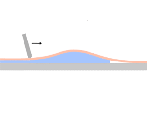
Figure 1 illustrates a liquid blister forced to advance between a thin elastic sheet and a rigid substrate by the action of a rigid frictionless blade moving at constant velocity  $v$, while enforcing a constant gap
  $w_0$ at the blister back end. The elastic layer of thickness
  $h$ is characterised by flexural rigidity
  $D=Eh^{3}/12(1-\nu ^{2})$, where
  $E$ is Young's modulus and
  $\nu$ is Poisson's ratio. The fluid is assumed to be incompressible and Newtonian with viscosity
  $\mu$. Ahead of the blister, the elastic sheet adheres to the substrate. The strength of the interface is characterised by adhesion energy
  $G_{c}$, whose dissipation is assumed to be localised at the separation front. The blister consists of a fluid-filled part and a cavity at the front filled with fluid vapours, which is at negative pressure
  $-\sigma _{0}$, with the atmospheric pressure taken as reference. There is therefore a lag between the separation front and the fluid front. A residual fluid film trapped between the sheet and the substrate is left behind the blister. This region, assumed to be infinite, is referred to as the tail.

Figure 1. Liquid blister trapped between an elastic sheet and a rigid substrate. The blister is driven by a steadily moving blade, kinematically constrained to enforce a constant gap  $w_0$ at the receding back end of the blister. A negative pressure
  $-\sigma _0$ acts in the lag cavity behind the separation front.
Although the existence of fluid lag at the front end of the blister is a requirement to avoid a pressure singularity incompatible with the underlying mathematical model, a gap  $w_{0}$ is required at the receding end of the blister, where the blade touches the elastic sheet, to regularise the pressure singularity that would otherwise arise. Both the fluid lag
  $\lambda$ and the residual gap
  $w_{\infty }$ far behind the blade are a priori unknown and thus part of the solution.
The blister is characterised by three moving boundaries: a separation front where the elastic layer breaks away from the substrate, a fluid front lagging behind the separation front and a receding front at the blade. In the moving coordinate system with origin at the blade,  $x=X-vt$, where
  $X$ is a fixed coordinate and
  $t$ is time, the separation front is located at
  $x=\ell (t)$, the fluid front at
  $x=\ell _{f}(t)$, with
  $\ell _{f}=\ell -\lambda$. The geometry of the blister and of the tail is described by the gap thickness
  $w(x,t)$, which also represents the deflection of the elastic sheet.
The force  $\boldsymbol {F}$ imparted by the frictionless blade pressing down on the sheet to squeeze the fluid forward is normal to the neutral axis of the sheet. As the slope of the elastic sheet at the point of contact is
  $w^{\prime }(0,t)>0$, the horizontal component
  $H$ of force
  $\boldsymbol {F}$ can be expressed as
  $H=Vw^{\prime }(0,t)$, where
  $V$ the vertical component given by
  $V=D(w^{\prime \prime \prime }(0^{-},t)-w^{\prime \prime \prime }(0^{+},t))$ within the approximation of Euler–Bernoulli beam theory. When the blister propagates, the external power
  $Hv$ balances the dissipation at the propagation front, which is associated with the delamination of the sheet from the substrate, the dissipation in the viscous fluid and the rate of change of the elastic energy in the sheet.
In summary, the set of parameters  $\mathcal {S}$ defining the moving blister problem consists of the blade velocity
  $v$, the imposed gap
  $w_{0}$ at the blade, the adhesion energy
  $G_{c}$, the bending stiffness
  $D$, the viscosity
  $\mu$ and the negative lag pressure
  $-\sigma _{0}$. Clearly, the problem is time dependent and its solution requires the initial conditions be defined. However, the solution eventually reaches a quasi-steady state in the limit
  $w_{0} \rightarrow 0$, with the volume of fluid in the blister remaining approximately constant.
2.2. Governing equations
To complete the description of the problem, we introduce fluid pressure  $p(x,t)$ and fluid flux
  $q(x,t)$ measured relative to the fixed coordinate
  $X$. In the lag region
  $\ell _{f}< x<\ell$, the vapour pressure is
  $p=-\sigma _{0}$, recalling that the atmospheric pressure is taken as reference. The fluid pressure vanishes sufficiently far behind the blade in order to satisfy static equilibrium between the fluid film and the elastic sheet.
The equations governing the unknown fields in both the blister and the tail, as well as the evolution of the blister length  $\ell$ and of the fluid lag
  $\lambda =\ell -\ell _{f}$ are formulated in the moving coordinate system attached to the blade. The elastic sheet is viewed as a Euler–Bernoulli beam and thus its deflection
  $w(x,t)$ is related to the net pressure
  $p$ according to
 \begin{equation} D\frac{\partial^{4}w}{\partial x^{4}}=p,\quad x\in[-\infty,\ell]\end{equation}
noting that  $p=-\sigma _{0}$ in the lag region
  $\ell _{f}< x\le \ell$. The flow of fluid in the moving blister is assumed to be governed by lubrication theory. Within this description, the continuity equation written in the moving coordinate system yields
 \begin{equation} \frac{\partial w}{\partial t}-v\frac{\partial w}{\partial x}+\frac{\partial q}{\partial x}=0,\quad x\in[-\infty,\ell_{f}] \end{equation}
and Poiseuille law reads
 \begin{equation} q={-}\frac{w^{3}}{\mu'}\frac{\partial p}{\partial x}, \end{equation}
where  $\mu '=12\mu$ is introduced to remove numerical factors from the scales defined in § 3.
These three equations together with the initial gap profile and the following conditions on  $w(x,t)$ constitute a closed system of equations to determine the blister thickness
  $w(x,t)$, length
  $\ell (t)$ and lag
  $\lambda (t)$ as functions of the parameter set
  $\mathcal {S}$.
2.2.1. At the delamination front  $x=\ell$

The geometrical conditions are
 \begin{equation} w=\frac{\partial w}{\partial x}=0, \end{equation}
and the separation criterion is
 \begin{equation} \frac{\partial^{2}w}{\partial x^{2}}=\left(\frac{2G_{c}}{D}\right)^{1/2}. \end{equation}
The second condition (2.4) results from the assumption that the substrate is rigid and that the delamination is localised at the moving front. The separation condition (2.5) expresses the curvature at the peeling front in terms of the ratio of the critical energy release rate and the bending stiffness (Landau & Lifshitz Reference Landau and Lifshitz1986; Hutchinson & Suo Reference Hutchinson and Suo1991; Majidi & Adams Reference Majidi and Adams2009).
2.2.2. At the fluid front ($x=\ell _{f}$)

The movement of the fluid front is determined by the Stefan condition
 \begin{equation} v+\frac{\mathrm{d}\ell_f}{\mathrm{d}t}=\frac{q}{w}. \end{equation}
There are five continuity conditions
 \begin{equation} \left[\frac{\partial^{i}w}{\partial x^{i}}\right]=0,\quad i=0,\ldots,4,\end{equation}
where  $[f(\ell )]=f(x)|_{x=\ell _{f}^{+}}-f(x)|_{x=\ell _{f}^{-}}$. In particular, continuity of the fourth-order derivative represents continuity of the pressure at the fluid front, i.e.
  $p(\ell _{f})=-\sigma _{0}$.
2.2.3. In the receding region ($x \leq 0$)

The aperture at the blade is known,
 \begin{equation} w=w_{0},\quad x=0. \end{equation}
With the net pressure vanishing far behind the blister, the gap tends to a constant but unknown value  $w_\infty (t)$,
 \begin{equation} w=w_{\infty}\left(t\right),\quad x\rightarrow-\infty. \end{equation}
 Once  $w(x,t)$ has been determined by solving the system of (2.4)–(2.8), the components of the force
  $\boldsymbol {F}$ applied by the blade, normal and parallel to its motion can be deduced from the slope of the deflection and the jump of the shear force at
  $x=0$.
2.3. Long blister limit
The asymptotic solution for a long blister is characterised by the existence of a central region with a quasi-uniform pressure, to which are appended two boundary layers: one at the front of the blister, the other at the back. The boundary layers can be considered as being quasi-autonomous and can thus be approximated as a travelling wave. However, in the limiting case  $w_{0} \rightarrow 0$, the whole solution is in the form of a travelling wave, after undergoing some transient evolution from an initial state at rest.
This structure of the long-blister asymptotic solution rests on two key points. First, the matched curvature between the front-end boundary layer and the core region is the same as the matched curvature at the back-end boundary layer, a consequence of the front–back symmetry of the outer solution resulting in part from the uniformity of the pressure in the central region. Second, the velocity  $v'$ of the separation front and of the fluid front is to first order the same as the velocity
  $v$ of the blade. Actually, as demonstrated in Appendix A,
  $v'=(1-\epsilon (t))v$, where
  $\epsilon \sim w_{\infty }\ell ^{-2}$, noting that
  $w_{\infty } \rightarrow 0$ and thus
  $v'\rightarrow v$ in the limit
  $w_{0}\rightarrow 0$. Thus, although the blister progressively contracts as it is bleeding fluid through the gap at the blade, the solutions in the boundary layers are to first order translationally time invariant.
The outer solution of the central region couples the two boundary layers: the back imposes the front velocity, but the front imposes the matched curvature at the back, which ultimately controls the force on the blade under certain conditions. With the matched curvature remaining constant to first order, the uniform pressure in the core region of the blister varies according to  $p\sim \ell ^{-2}$ (this dependence of
  $p$ on the blister length could be translated into a dependence on time
  $t$, on account that the bleeding rate is to first order constant in the long-blister asymptotic case).
In the boundary layers, the continuity equation (2.2) can therefore be simplified to
 \begin{equation} v\frac{\mathrm{d}w}{\mathrm{d}x}=\frac{\mathrm{d}q}{\mathrm{d}x}. \end{equation}
Integrating this equation yields
 \begin{equation} q=v w \end{equation}
in the front-end boundary layer, but
 \begin{equation} q=v(w-w_{\infty}) \end{equation}
in the back-end boundary layer. The difference between these two integrated continuity equations stems from the Stefan condition at the front and the zero flux condition at  $x\rightarrow -\infty$. Combining the Euler–Bernoulli equation (2.1) with Poiseuille's law (2.3) and either (2.11) or (2.12) yields a fifth-order nonlinear ordinary differential equation (ODE) governing the gap
  $w(x)$ in the fluid-filled part of the front layer and in the back layer.
3. Scaling
The structure of the asymptotic solution for a long blister, a central region under quasi-uniform pressure, sandwiched between two boundary layers, is confirmed by a scaling analysis, which further shows that the solution in the boundary layers actually depends on two numbers: toughness  $\mathcal {K}$ and imposed gap
  $\mathcal {W}$ at the blade. As the focus of this study is to determine the quasi-stationary force required to drive the blade, we avoid conducting a scaling analysis of the general set of equations by considering the limiting case
  $w_0 \rightarrow 0$, which accepts a travelling-wave solution. The back-end boundary layer in the general case
  $w_0>0$ then naturally depends on the additional number
  $\mathcal {W}$.
Let  $\ell _*$ and
  $w_*$ denote scales for the blister length and thickness, respectively. We then define the dimensionless gap
  $\varOmega$, coordinate
  $\xi$, fluid front position
  $\gamma _{f}$ and lag
  $\varLambda$
 \begin{equation} \quad\varOmega=\frac{w}{\gamma_{f}^{\alpha}w_*},\quad \xi=\frac{x}{\ell_{f}},\quad\gamma_{f}=\frac{\ell_{f}}{\ell_*},\quad \varLambda=\frac{\ell-\ell_{f}}{\ell_*}=\frac{\lambda}{\ell_*}. \end{equation}
Considering the limiting case  $w_0=0$, for which the solution is only defined on
  $x \in [0,\ell ]$, and assuming that
  $\ell _f$ is used as proxy for the volume of fluid trapped in the blister (because a one-to-one relationship exists between these two parameters), the nonlinear system of equations governing
  $\varOmega (\xi )$ at steady state are
 \begin{gather} \varOmega^{2}\frac{\mathrm{d}^{5}\varOmega}{\mathrm{d}\xi^{5}} ={-}\mathcal{G}_{m}\gamma_{f}^{5-3\alpha},\quad\xi\in\left[0,1\right],\end{gather}
 \begin{gather} \frac{\mathrm{d}^{4}\varOmega}{\mathrm{d}\xi^{4}} ={-}\mathcal{G}_{s}\gamma_{f}^{4-\alpha}, \quad\xi\in\left[1,1+\frac{\varLambda}{\gamma_{f}}\right],\end{gather}
 \begin{gather} \varOmega = \frac{\mathrm{d}\varOmega}{\mathrm{d}\xi}=0,\quad \frac{\mathrm{d}^{2}\varOmega}{\mathrm{d}\xi^{2}}=\mathcal{G}_{k}\gamma_{f}^{2-\alpha},\quad \mathrm{at}\; \xi=1+\frac{\varLambda}{\gamma_{f}}, \end{gather}
 \begin{gather} \varOmega=0,\quad \mathrm{at}\ \xi=0. \end{gather}
Three dimensionless groups appear in the above equations:
 \begin{equation} \mathcal{G}_{m}=\frac{\mu'v\ell_*^{5}}{Dw_*^{3}},\quad \mathcal{G}_{k}=\left(\frac{2G_{c}\ell_*^{4}}{Dw_*^{2}}\right)^{1/2},\quad \mathcal{G}_{s}=\frac{\sigma_{0}\ell_*^{4}}{w_*D}. \end{equation}
The scales  $\ell _*$ and
  $w_*$ are identified by imposing
  $\mathcal {G}_{m}=\mathcal {G}_{s}=1$. This particular choice of scaling makes it possible to consider the limiting case
  $G_c=0$. Hence,
 \begin{equation} \ell_*=\left(\frac{\mu'vD^{2}}{\sigma_{0}^{3}}\right)^{1/7},\quad w_*=\left(\frac{\mu'^{4}v^{4}D}{\sigma_{0}^{5}}\right)^{1/7}, \end{equation}
and the scale  $k_*$ for the curvature is therefore
 \begin{equation} k_*=\left(\frac{\mu'^{2}v^{2}\sigma_{0}}{D^{3}}\right)^{1/7}. \end{equation}
In addition, choosing
 \begin{equation} \alpha=2\end{equation}
guarantees that  $\varOmega$ remains bounded when
  $\gamma _{f}\rightarrow \infty$. Indeed, for this limit, the right-hand side of (3.2) vanishes (equivalent to an inviscid fluid), (3.3) effectively disappears as
  $\varLambda \rightarrow 0$,
  $\varOmega (1)\rightarrow 0$ and importantly the curvature tends to a finite limit at
  $\xi =1$.
Using the Euler–Bernoulli equation (2.1) and the continuity equation (2.11), the net pressure and flux scale according to
 \begin{equation} \varPi=\frac{\gamma_{f}^{2}p}{p_*},\quad\varPsi=\frac{q}{\gamma_{f}^{2}q_*}, \end{equation}
with the scales  $p_*$ and
  $q_*$ given by
 \begin{equation} p_*=\sigma_{0},\quad q_*=\left(\frac{\mu'^{4}v^{11}D}{\sigma_{0}^{5}}\right)^{1/7}. \end{equation}
The above expressions for  $\varPi$ and
  $\varPsi$ guarantee that the scaled versions of (2.1) and (2.2) become
 \begin{equation} \frac{\mathrm{d}^{4}\varOmega}{\mathrm{d}\xi^{4}}=\varPi, \quad\varPsi=\varOmega. \end{equation}
 Finally, the horizontal component  $H$ and the vertical component
  $V$ of the force on the blade scale according to
 \begin{equation} \mathring{\mathcal{H}}=\frac{H}{H_{*}},\quad \mathring{\mathcal{V}}=\frac{\gamma_f V}{ V_{*}}, \end{equation}
with the scales  $H_{*}$ and
  $V_{*}$ given by
 \begin{equation} H_{*}=\left(\mu'^{4}v^{4}D\sigma_{0}^{2}\right)^{1/7},\quad V_{*}=\left(\mu'vD^{2}\sigma_{0}^{4}\right)^{1/7}. \end{equation}
The scaling of the vertical force  $V$ is consistent with that of the net pressure, i.e.
  $V_{*} = \ell_{*} p_{*}$. It implies that for a long blister, the vertical force essentially equilibrates the pressure at the back end of the blister.
The remaining free number  $\mathcal {G}_{k}$ in the original set (3.6a–c) can be interpreted as a dimensionless toughness; it is renamed as
  $\mathcal {K}$. For non-zero
  $w_{0}$, there is an additional number
  $\mathcal {W}=w_0/w_*$ controlling the back-end boundary layer. The front-end boundary layer only depends on
  $\mathcal {K}$, however, as the only information from the back end affecting its solution is the velocity
  $v$ of the blade. In § 4.4, it is shown that the back-end boundary layer actually depends on a single number, a function of both
  $\mathcal {K}$ and
  $\mathcal {W}$. The explicit expressions of these two numbers in terms of the physical quantities defining the blister problem are given by
 \begin{equation} \mathcal{\mathcal{K}}=\left(\frac{2^{7}G_{c}^{7}}{D\sigma_{0}^{2}\mu'^{4}v^{4}}\right)^{1/14},\quad\mathcal{W}=\left(\frac{w_{0}^{7}\sigma_{0}^{5}}{\mu'^{4}v^{4}D}\right)^{1/7}. \end{equation}
4. Long-blister limit
4.1. Structure of solution
As noted earlier, the dimensionless viscosity effectively vanishes in the interval  $\xi \in [0,1]$ and the lag
  $\varLambda /\gamma _{f}$ tends to zero (noting that
  $\varLambda =O(1)$ or less, see following) for large
  $\gamma _{f}$. Viewed at length scale
  $\ell _{f}=\gamma _{f}\ell _*$, this solution is characterised by a uniform pressure
  $\mathring {\varPi }$. However, there exist two boundary layers, one at the advancing front and the other at the receding end of the blister, where viscous dissipation cannot be neglected, see figure 2. The solution in these (three) regions will be expressed as
  $\hat {\varOmega }(\hat {\xi })$ for the front-end boundary layer,
  $\mathring {\varOmega }(\xi )$ for the core region, and
  $\check {\varOmega }(\check {\xi })$ for the back-end boundary layer. The boundary-layer solutions and the outer solution are matched with the curvature, which is equal to
  $\varUpsilon (\mathcal {K})$ at both ends of the core region owing to the symmetric nature of the outer solution.

Figure 2. Structure of solution: (a) outer solution, (b) back-end boundary layer, (c) front-end boundary layer and (d) schematic of the regions of validity of the inner and outer solutions in the matching procedure.
4.2. Front-end boundary layer
The boundary layer at the moving front is representative of the tip region of any propagating near-surface hydraulic fracture, provided that there is a separation of scales. The solution is expressed as  $\hat {\varOmega }(\hat {\xi })$, where
 \begin{equation} \hat{\xi}=(\ell-x)/\ell_*, \quad \hat{\varOmega}=w/w_*, \end{equation}
with the scales defined in (3.7a,b). The solution is characterised by a lag  $\varLambda$, which, in the context of the moving blister, is equal to
  $\varLambda =(\ell -\ell _{f})/\ell _*$. Its maximum value
  $\varLambda _{max}=1.325$ is reached in the limit
  $\mathcal {K}=0$ (Wang & Detournay Reference Wang and Detournay2018). The far-field curvature
  $\varUpsilon (\mathcal {K})$ is defined as
 \begin{equation} \varUpsilon = \lim_{\hat{\xi}\rightarrow\infty}\hat{\varOmega}'', \end{equation}
where the prime denotes differentiation with respect to the argument of the function. Plots of the functions  $\varUpsilon (\mathcal {K})$ and
  $\varLambda (\mathcal {K})$ are shown in figure 3. Since the curvature is matched between the outer solution and the front-end boundary layer,
  $\varUpsilon (\mathcal {K})$ effectively represents the dimensionless toughness for the outer solution. This apparent toughness accounts not only for the energy expended in delamination at the front, but also for the resistance to propagation associated with the presence of a lag and for viscous dissipation in the tip region.

Figure 3. Front-end boundary layer: (a) far-field curvature  $\varUpsilon$ and (b) lag
  $\varLambda$; numerical solution (solid line) and asymptotic solution (dashed lines) (Wang & Detournay Reference Wang and Detournay2018).
There are two limiting regimes of propagation (Ball & Neufeld Reference Ball and Neufeld2018; Wang & Detournay Reference Wang and Detournay2018): a toughness-dominated regime ( $\mathcal{K} >rsim 10$), and a viscosity-dominated regime (
 $\mathcal{K} \lesssim 0.1$). The asymptotic behaviours of
  $\varUpsilon (\mathcal {K})$ for small and large
  $\mathcal {K}$ are given by
 \begin{equation} \varUpsilon\simeq\mathcal{K},\quad\mathcal{K}>rsim 10\quad \textrm{and} \quad \varUpsilon\simeq1.769,\quad\mathcal{K}\lesssim0.1 \end{equation}
and in the range  $0.1<\mathcal {K}<10,$
  $\varUpsilon (\mathcal {K})$ is conveniently approximated as (Wang & Detournay Reference Wang and Detournay2018)
 \begin{equation} \varUpsilon\simeq\sum_{i=0}^{4}a_{i}\mathcal{K}^{i},\quad0.1<\mathcal{K}<10, \end{equation}
where  $a_{0}=1.70404$,
  $a_{1}=0.09348$,
  $a_{2}=0.21373$,
  $a_{3}=-0.02278$ and
  $a_{4}=8.87789\times 10^{-4}$.
4.3. Outer solution
The solution in the bulk of the blister, the outer solution, is denoted as  $\mathring {\varOmega }(\xi )$ and
  $\mathring {\varPi }$. These field variables are scaled similarly to
  $\varOmega (\xi )$ and
  $\varPi (\xi )$. The outer solution is obtained by solving
 \begin{equation} \mathring{\varOmega}'''' =\mathring{\varPi},\quad\xi\in\left[0,1\right], \end{equation}
with conditions
 \begin{gather} \mathring{\varOmega}=\mathring{\varOmega}' =0,\quad\mathring{\varOmega}''=\varUpsilon(\mathcal{K}),\quad\mathrm{at}\ \xi=1, \end{gather}
 \begin{gather} \mathring{\varOmega}=0,\quad \mathring{\varOmega}' =0,\quad\mathrm{at}\ \xi=0. \end{gather}
The solution is given by
 \begin{equation} \mathring{\varOmega}=\frac{\mathring{\varPi}}{24}\xi^{2}(1-\xi)^{2}, \quad\mathring{\varPi}=12\,\varUpsilon(\mathcal{K}). \end{equation}
The condition on the curvature at  $\xi =1$ is the matching condition between the outer solution and the front-end boundary layer. Because of the symmetry in
  $\mathring {\varOmega }(\xi )$, the curvature at
  $\xi =0$ is also equal to
  $\varUpsilon (\mathcal {K})$. The curvature is further used to match the outer solution and the boundary-layer solution at the back end.
Although the curvature scale does not depend on  $\gamma _f$, this dimensionless parameter enters the scales used to define
  $\xi$,
  $\mathring {\varOmega }$ and
  $\mathring {\varPi }$. The blister thickness
  $w$ and pressure
  $p$ evolve therefore with time because
  $\gamma _f$ decreases with
  $t$ owing to the bleeding of the blister when
  $w_0 >0$. However, the curvature at both ends of the blister is quasi-time-invariant as long as
  $\gamma _f$ is large enough to guarantee that the front velocity
  $v' \simeq v$.
4.4. Back-end boundary layer
For the receding end of the blister, we introduce the fast variable  $\check {\xi }$ and the associated blister thickness
  $\check {\varOmega }(\check {\xi })$ and pressure
  $\check {\varPi }(\check {\xi })$
 \begin{equation} \check{\xi}=\varUpsilon^{3}(\mathcal{K})\frac{x}{\ell_{*}},\quad\check{\varOmega}=\varUpsilon^{5}(\mathcal{K})\frac{w}{w_{*}},\quad\check{\varPi}=\varUpsilon^{{-}7}(\mathcal{K})\frac{p}{p_{*}}. \end{equation}
 In this scaling, the horizontal force  $\check {\mathcal {H}}$ and the vertical force
  $\check {\mathcal {V}}$ applied by the blade are naturally defined as
 \begin{equation} \check{\mathcal{H}}=\varUpsilon^{{-}2}(\mathcal{K})\frac{H}{H_{*}},\quad\check{\mathcal{V}}=\varUpsilon^{{-}4}(\mathcal{K})\frac{V}{V_{*}}, \end{equation}
so that  $\check {\mathcal {H}}=-\check {\varOmega '}(0)[\check {\varOmega }'''(0)],\;\check {\mathcal {V}}=-[\check {\varOmega }'''(0)]$. The receding boundary layer and the outer solution are matched with the curvature, i.e.
 \begin{equation} \lim_{\xi\rightarrow0}\mathring{\varOmega}''=\varUpsilon(\mathcal{K})\lim_{\check{\xi}\rightarrow\infty}\check{\varOmega}'', \end{equation}
which implies that
 \begin{equation} \check{\varOmega}=\tfrac{1}{2}\check{\xi}^{2},\quad\check{\xi}\rightarrow\infty. \end{equation}
With the introduction of  $\varUpsilon$ in the definition of the boundary-layer variables, the system of equations governing
  $\check {\varOmega }(\check {\xi })$ only depends on
  $\check {\varOmega }_{0}$, the scaled gap at the blade
 \begin{equation} \check{\varOmega}_{0}=\mathcal{W}\varUpsilon^{5}(\mathcal{K}). \end{equation}
 The boundary layer consists of two parts: the back end of the blister corresponding to  $\check {\xi }\in [0,\infty ]$ and the tail behind the blade,
  $\check {\xi }\in [-\infty ,0]$. It can be deduced from (2.3) and (2.12) that the gap
  $\check {\varOmega }(\check {\xi })$ in the boundary layer is governed by
 \begin{equation} \check{\varOmega}^{3}\check{\varOmega}'''''={-}(\check{\varOmega}-\check{\varOmega}_{\infty}), \quad\check{\xi}\in\left[-\infty,\infty\right],\end{equation}
subject to the conditions
 \begin{gather} \check{\varOmega}= \tfrac{1}{2} \check{\xi}^2 \quad\mathrm{as}\ \check{\xi}\rightarrow\infty, \end{gather}
 \begin{gather} \check{\varOmega}=\check{\varOmega}_{0}\quad\mathrm{at}\ \check{\xi}=0,\end{gather}
 \begin{gather} \check{\varOmega}=\check{\varOmega}_{\infty}\quad\mathrm{as}\ \check{\xi}\rightarrow-\infty. \end{gather}
 The system of (4.14)–(4.17) is closed as there are enough constraints to identify the five constants of integration for (4.14), the discontinuity of  $\check {\varOmega }'''(\check {\xi })$ at
  $\check {\xi }=0$ and the residual gap
  $\check {\varOmega }_{\infty }$. Indeed, (4.15) implies that
  $\check {\varOmega }''=1$ and
  $\check {\varOmega }'''=\check {\varOmega }''''=0$ at
  $\check {\xi }=\infty$, while (4.17) entails the vanishing of the derivatives of
  $\check {\varOmega }(\check {\xi })$ at
  $\check {\xi }=-\infty$.
Numerical solution of the system of (4.14)–(4.17) is facilitated by recognising that the governing equation (4.14) for the gap degenerates into a linear ODE at sufficiently large distance behind the blade
 \begin{equation} \check{\varOmega}_{\infty}^{3}\check{\varOmega}'''''={-}(\check{\varOmega}-\check{\varOmega}_{\infty}),\quad -\check{\xi}\gg 1. \end{equation}
After dropping the terms that become unbounded as  $\check {\xi }\rightarrow -\infty$, the asymptotic solution is thus given by
 \begin{equation} \check{\varOmega}=\check{\varOmega}_{\infty}+\left[\check{c}_{1}\cos\left(\frac{\alpha\check{\xi}}{\check{\varOmega}_{\infty}^{3/5}}\right)+\check{c}_{2}\sin\left(\frac{\alpha\check{\xi}}{\check{\varOmega}_{\infty}^{3/5}}\right)\right]\exp\left(\frac{\beta\check{\xi}}{\check{\varOmega}_{\infty}^{3/5}}\right),\quad -\check{\xi}\gg 1, \end{equation}
where
 \begin{equation} \alpha=\sqrt{\frac{5}{8}-\frac{\sqrt{5}}{8}},\quad\beta=\left(\frac{1}{4}+\frac{\sqrt{5}}{4}\right). \end{equation}
The above asymptotic solution replaces the boundary condition (4.17) at  $\check {\xi }=-\infty$. Now nine conditions are needed to obtain a solution: five to integrate the ODE, one to determine
  $[\check {\varOmega }'''(0)]$ and three to identify the unknowns
  $\check {\varOmega }_{\infty }$,
  $\check {c}_{1}$, and
  $\check {c}_{2}$ of the asymptotic solution. These requirements are fulfilled by the three conditions equivalent to (4.15) as
  $\check {\xi }\rightarrow \infty$, one constraint at
  $\check {\xi }=0$ and five continuity conditions with the asymptotic solution (4.19), namely the function
  $\check {\varOmega }(\check {\xi })$ and its first four derivatives at the truncated boundary.
The solution in the back-end boundary layer is obtained numerically by combining a finite-element discretisation of the beam equation and a finite-volume discretisation of the lubrication equation. The general algorithm is the same as the one used to solve the front-end boundary layer, see Wang & Detournay (Reference Wang and Detournay2018) for details. The infinite fluid-filled channel is truncated to the interval  $\check {\xi }\in [\check {\xi }_{-\infty },\check {\xi }_{\infty }]$, where
  $\check {\xi }_{-\infty }$ and
  $\check {\xi }_{\infty }$ are chosen, through a trial-and-error procedure, to be large enough to ensure convergence of the solution. The finite region is divided into
  $n$ elements that are delimited by
  $n+1$ nodes with coordinate
  $\check {\xi }_{i}$,
  $i=1,\ldots ,n+1$. One node is located at
  $\check {\xi }=0$ enabling us to impose the constraint
  $\check {\varOmega }(0)=\check {\varOmega }_{0}$. Net pressure
  $\check {\varPi }_{i}$, aperture
  $\check {\varOmega }_{i}$ and aperture gradient
  $\check {\varOmega }_{i}^{\prime }$ are the primarily variables defined at each node
  $i=1,\ldots ,n+1$, while flux
  $\check {\varPsi }_{i+{1}/{2}}$ is evaluated at the midpoint of element
  $i$. The discretised fluid–beam equations and the boundary conditions constitute a system of
  $2n+2$ nonlinear algebraic equations in terms of
  $2n+2$ unknowns
  $\check {\varOmega }_{\infty }$,
  $\check {c}_{1}$,
  $\check {c}_{2}$,
  $\check {\varOmega }_{i}$,
 $\check {\varOmega }_{i}^{\prime }$,
  $i=2,\ldots ,n+1$ (except for the opening at
  $\check {\xi }=0$ ), noting that
  $\check {\varOmega }_{1}$,
 $\check {\varOmega }_{1}^{\prime }$ are determined by the constants
  $\check {\varOmega }_{\infty }$,
  $\check {c}_{1}$ and
  $\check {c}_{2}$. These nonlinear systems of equations are solved using Newton's iteration procedure built in the Mathematica software.
5. Small-, intermediate- and large-$\check {\varOmega }_{0}$ regimes

Motivated by the determination of the force on the blade, we focus our attention to the structure of the solution near the origin. As evident from the system of (4.14)–(4.17), the scaled solution in the back-end boundary layer depends on only one number, the prescribed gap  $\check {\varOmega }_{0}=\mathcal {W}\varUpsilon ^{5}(\mathcal {K})$ at the blade edge. In principle, we can identify three regimes: (i) a small-
 $\check {\varOmega }_{0}$ asymptote, which only depends on the viscous dissipation in the receding boundary layer; (ii) an intermediate-
 $\check {\varOmega }_{0}$ regime; (iii) a large-
 $\check {\varOmega }_{0}$ asymptote for which the curvature in front of the blade is equal to the matched curvature between the front-end boundary layer and the bulk solution.
5.1. Small-$\check {\varOmega }_{0}$ regime

If  $\check {\varOmega }_{0}=0$, the blister thickness
  $\check {\varOmega }(\check {\xi })$ near
  $\check {\xi }=0$ is given by (Tayler & King Reference Tayler and King1987)
 \begin{equation} \check{\varOmega}\overset{\check{\xi}\rightarrow0}{\sim}A\check{\xi}^{5/3}, \end{equation}
with
 \begin{equation} A=\frac{1}{2}\left(\frac{3^{5}}{5\times7}\right)^{1/3}\simeq0.9539 \end{equation}
as it can be confirmed by substituting this power-law solution into (4.14).
When  $\check {\varOmega }_{0}\ll 1$,
  $\check {\varOmega }=A\check {\xi }^{5/3}$ becomes an intermediate asymptotic. To determine the solution near the origin, the problem can be rescaled so that this asymptote applies to the far field in the rescaled variable. This is done by introducing the new scaling
 \begin{equation} \tilde{\xi}=\check{\varOmega}_{0}^{{-}3/5}\check{\xi},\quad\tilde{\varOmega}=\check{\varOmega}_{0}^{{-}1}\check{\varOmega},\quad\tilde{\varPi}=\check{\varOmega}_{0}^{7/5}\check{\varPi}. \end{equation}
 The gap aperture  $\tilde {\varOmega }(\tilde {\xi })$ is then governed by
 \begin{equation} \tilde{\varOmega}^{3}\tilde{\varOmega}'''''={-}(\tilde{\varOmega}-\tilde{\varOmega}_{\infty}), \quad\tilde{\xi}\in\left[-\infty,\infty\right],\end{equation}
with conditions
 \begin{gather} \tilde{\varOmega}\overset{\tilde{\xi}\rightarrow\infty}{\sim}A\tilde{\xi}^{5/3},\end{gather}
 \begin{gather} \tilde{\varOmega}=1\quad\mathrm{at}\;\tilde{\xi}=0,\end{gather}
 \begin{gather} \tilde{\varOmega}=\tilde{\varOmega}_{\infty}+\left[\tilde{c}_{1}\cos\left(\frac{\alpha\tilde{\xi}}{\tilde{\varOmega}_{\infty}^{3/5}}\right)+\tilde{c}_{2}\sin\left(\frac{\alpha\tilde{\xi}}{\tilde{\varOmega}_{\infty}^{3/5}}\right)\right]\exp\left(\frac{\beta\tilde{\xi}}{\tilde{\varOmega}_{\infty}^{3/5}}\right),\qquad - \tilde{\xi}\gg 1, \end{gather}
where  $\tilde {\varOmega }_{\infty }=\check {\varOmega }_{\infty }/\check {\varOmega }_{0}$ is an a priori unknown number (smaller than 1). In other words,
  $\check {\varOmega }_{\infty }$ is simply proportional to
  $\check {\varOmega }_{0}$ in the asymptotic small-
 $\check {\varOmega }_{0}$ regime.
The system of (5.4)–(5.7) is solved numerically using an approach similar to that described in § 4.4. The asymptotic solution (5.5) is replaced by imposing the second, third and fourth derivative of (5.5) at a point  $\tilde {\xi }_{\infty }\gg 1$. Point
  $\tilde {\xi }_{\infty }$ must be chosen in such a way that the computed
  $\tilde {\varOmega }$ matches (5.5) in the neighbourhood of
  $\tilde {\xi }_{\infty }$. A similar approach is used for the continuity conditions between the computed
  $\tilde {\varOmega }$ and (5.7), which is enforced at a point
  $-\tilde {\xi }_{\infty }\gg 1$. Numerical solution of (5.4)–(5.7) yields
  $\tilde {\varOmega }_\infty =0.6125$,
  $\tilde {\varOmega }'(0)=0.8558$,
  $\tilde {\varOmega }''(0)=1.195$,
  $[\tilde {\varOmega }'''(0)]=-1.430$ and
  $\tilde {\varOmega }''''(0)=0.3732$.
The small- $\check {\varOmega }_{0}$ asymptotic solution is illustrated in figure 4 (
 $\tilde {\varOmega }(\tilde {\xi })$,
  $\tilde {\varOmega }''(\tilde {\xi })$,
  $\tilde {\varOmega }'''(\tilde {\xi })$ and
  $\tilde {\varOmega }''''(\tilde {\xi })$) in a linear scale near the origin to capture the solution behind the blade and in double logarithmic scale to illustrate convergence of the solution to the intermediate asymptote (5.5) in the back end of the blister. These figures indicate that the asymptotic solution (5.7) is effectively reached at
  $\tilde {\xi }\simeq -4$, and that the numerical solution matches the intermediate asymptote (5.5) at approximately
  $\tilde {\xi }\simeq 10$. In particular, note that the minimum gap
  $\tilde {\varOmega }_{min}=0.5495$ is located at
  $\tilde {\xi }_{min}=-1.566$. The peak pressure occurs at
  $\tilde {\xi }=-0.8052$, which marks the transition between forward and backward average flow.

Figure 4. Numerical (solid line) and asymptotic (dashed line) small- $\check {\varOmega }_{0}$ solutions near the back end: (a,b) gap
  $\tilde {\varOmega }(\tilde {\xi })$ and curvature
  $\tilde {\varOmega }^{\prime \prime }(\tilde {\xi })$; (c,d) shear force
  $\tilde {\varOmega }^{\prime \prime \prime }(\tilde {\xi })$ and net fluid pressure
  $\tilde {\varOmega }^{\prime \prime \prime \prime }(\tilde {\xi })$.
There is another solution operating on the scale of the variable  $\check {\xi }$ that connects the (intermediate) asymptote (5.1) to the far-field quadratic condition (4.12). This solution would need to be computed numerically. However, the intermediate asymptote (5.1) effectively shields the solution
  $\tilde {\varOmega }(\tilde {\xi })$ from (4.12), and thus from the processes at the front of the blister. In other words, the reaction force on the blade only depends on the viscous dissipation at the back end of the blister in the small-
 $\check {\varOmega }_{0}$ regime.
5.2. Large-$\check {\varOmega }_{0}$ regime

In the large- $\check {\varOmega }_{0}$ regime, viscous dissipation is expected to be negligible in the neighbourhood of the blade. Completely ignoring viscous effects, which implies a zero net pressure, would cause, however, the elastic sheet to contact the rigid substrate at some distance behind the blade (see the outer solution illustrated in the inset of figure 5a). However, as indicated earlier, the viscous dissipation associated with the narrowing of the gap leads to an increase of the fluid pressure. Complete closure of the gap is actually prevented, as it would entail a strong pressure singularity according to (5.1). This contradiction suggests the existence of an asymptotic viscous layer inside the back-end boundary layer, with the zero-viscosity solution acting as an outer solution.

Figure 5. Numerical (solid line) and zero-order (dashed line) outer solution near the back end for large  $\check {\varOmega }_{0}$: (a)
  $\bar {\varOmega }(\bar {\xi })$, (b)
  $\bar {\varOmega }''(\bar {\xi })$, (c)
  $\bar {\varOmega }'''(\bar {\xi })$ and (d)
  $\bar {\varOmega }''''(\bar {\xi })$. Results calculated for
  $\check {\varOmega _{0}}=6.4\times 10^{7}$.
5.2.1. Outer solution
A rescaling of the boundary-layer variables is required to derive the zero-viscosity solution. After defining the new variables as
 \begin{equation} \bar{\xi}=\check{\varOmega}_{0}^{{-}1/2}\check{\xi},\quad\bar{\varOmega}=\check{\varOmega}_{0}^{{-}1}\check{\varOmega}, \end{equation}
so as to preserve the independence upon  $\check {\varOmega }_{0}$ of the constant curvature at infinity, the governing equation becomes
 \begin{equation} \bar{\varOmega}^{3}\bar{\varOmega}'''''={-}\check{\varOmega}_{0}^{{-}1/2}\left(\bar{\varOmega}-\bar{\varOmega}_{\infty}\right),\quad\bar{\xi}\in\left[-\infty,\infty\right], \end{equation}
with  $\bar {\varOmega }_{\infty }=\check {\varOmega }_{\infty }/\check {\varOmega }_{0}$. This equation indicates that the right-hand side is negligibly small and can thus be ignored provided that
  $\check {\varOmega }_{0}\gg 1$ and
  $\bar {\varOmega }$ is of order
  $O(1)$ or more. Noting the condition at infinity, the zero-order solution
  $\bar {\varOmega }_{(0)}(\bar {\xi })$ is obtained by solving
 \begin{equation} \bar{\varOmega}''''_{(0)}=0, \quad\bar{\xi}\in\left[\bar{\xi}_{c},\infty\right], \end{equation}
subjected to
 \begin{equation} \bar{\varOmega}''_{(0)}=1,\ \bar{\varOmega}'''_{(0)}=0\quad \mathrm{at}\ \bar{\xi}= \infty;\quad\bar{\varOmega}_{(0)}(0)=1; \quad \bar{\varOmega}_{(0)}=\bar{\varOmega}'_{(0)}=\bar{\varOmega}''_{(0)}=0\quad \mathrm{at}\ \bar{\xi}=\bar{\xi}_{c}. \end{equation}
In the above,  $\bar {\xi }_{c}<0$ is the a priori unknown position of the contact line where the elastic sheet would touch the substrate if the fluid were inviscid. This set of equations is closed since the six conditions (5.11a–c) provide the necessary information to determine the four constants of integration,
  $[\bar {\varOmega }'''_{(0)}(0)]$, and
  $\bar {\xi }_{c}$.
The zero-order solution  $\bar {\varOmega }_{(0)}(\bar {\xi })$ is readily obtained as
 \begin{equation} \bar{\varOmega}_{(0)}(\bar{\xi})=\begin{cases} 0, & \bar{\xi}\le-\bar{\xi}_{c},\\ \left(\dfrac{\bar{\xi}_c-\bar{\xi}}{\bar{\xi}_{c}}\right)^{3}, & \bar{\xi}_{c}\le\bar{\xi}\le0,\\ 1+\dfrac{\bar{\xi}}{2}\left(\bar{\xi}-\bar{\xi}_{c}\right), & \bar{\xi}\ge0, \end{cases}\end{equation}
with
 \begin{equation} \bar{\xi}_{c}={-}\sqrt{6}. \end{equation}
 The numerical solution of  $\bar {\varOmega }(\bar {\xi })$ in the large-
 $\check {\varOmega }_{0}$ regime, which is governed by equations similar to the system (5.4)–(5.7) except for the condition as
  $\bar {\xi }\rightarrow \infty$, is illustrated in figure 5(a), together with the zero-order solution (5.12). Comparison between the numerical and the zero-order solution for
  $\bar {\varOmega }''(\bar {\xi })$,
  $\bar {\varOmega }'''(\bar {\xi })$ and
  $\bar {\varOmega }''''(\bar {\xi })$ can be found in figure 5(c,d), noting that
  $\bar {\varOmega }''''_{(0)}(\bar {\xi })=0$. Figure 5 reveals the existence of a nested boundary layer near
  $\bar {\xi } = \bar {\xi }_c$.
5.2.2. Inner solution
Yet another scaling is required to determine the solution in the inner viscous layer at the back end for the large- $\check {\varOmega }_{0}$ regime, in particular the relationship between
  $\check {\varOmega }_{\infty }$ and
  $\check {\varOmega }_{0}$. Thus, let
 \begin{equation} \breve{\xi}=(\bar{\xi}-\bar{\xi}_{c})\check{\varOmega}_{0}^{\lambda},\quad\breve{\varOmega}=\bar{\varOmega}\check{\varOmega}_{0}^{\nu}, \end{equation}
where the exponents  $\lambda$ and
  $\nu$ (expected to be positive) are to be specified by requiring that the equations governing
  $\breve {\varOmega }(\breve {\xi })$ do not contain
  $\check {\varOmega }_{0}$. The information needed to determine these two power-law indices can be deduced from the rescaled governing equation
 \begin{equation} \check{\varOmega}_{0}^{5\lambda-3\nu+1/2}\breve{\varOmega}^{3}\breve{\varOmega}'''''={-}\left(\breve{\varOmega}-\breve{\varOmega}_{\infty}\right)\end{equation}
and the condition
 \begin{equation} \check{\varOmega}_{0}^{3\lambda-\nu}\breve{\varOmega}'''={-}\bar{\xi}_{c}^{{-}1}\quad \mathrm{as}\ \breve{\xi}\rightarrow\infty, \end{equation}
deduced by matching  $\bar {\varOmega }'''_{(0)}(0^{-})=-\bar {\xi }_{c}^{-1}$ as
  $\breve {\xi }\rightarrow \infty$. Except for the finite (unknown) condition
 \begin{equation} \breve{\varOmega}=\breve{\varOmega}_{\infty}\equiv\frac{\check{\varOmega}_{\infty}}{\check{\varOmega}_{0}}\check{\varOmega}_{0}^{\nu} \quad \mathrm{as}\ \breve{\xi}\rightarrow-\infty, \end{equation}
all the other conditions on  $\breve {\varOmega }(\breve {\xi })$ or its derivatives are either zero or infinite. Elimination of the exponents of
  $\check {\varOmega }_{0}$ in (5.15) and (5.16) requires
  $\lambda =1/8$ and
  $\nu =3/8$. These results further imply that
 \begin{equation} \check{\varOmega}_{\infty}=\breve{\varOmega}_{\infty}\check{\varOmega}_{0}^{5/8}. \end{equation}
 If the asymptotic solution (4.19), properly rescaled for  $\breve {\varOmega }(\breve {\xi })$, is used, there are eight unknowns:
  $\breve {\varOmega }_{\infty }$, the two constants of the asymptotic solution (4.19) and five constants of integration. The problem is closed by the five continuity conditions between the asymptotic solution (4.19) and
  $\breve {\varOmega }(\breve {\xi })$ and the asymptotic condition (5.16) as
  $\breve {\xi }\rightarrow \infty$. (The asymptotic condition can be construed as being equivalent to the three conditions
  $\breve {\varOmega }''(\breve {\xi }_{\infty })=-\bar {\xi }_{c}^{-1}\breve {\xi }_{\infty }$,
  $\breve {\varOmega }'''(\breve {\xi }_{\infty })=-\bar {\xi }_{c}^{-1}$ and
  $\breve {\varOmega }''''(\breve {\xi }_{\infty })=0$, with
  $\breve {\xi }_{\infty }$ denoting the truncated boundary, when constructing the solution numerically.) The numerical solution in this viscous boundary layer can be found in figure 6, together with the asymptotic solution. Numerical results show that
  $\breve {\varOmega }_{\infty }=2.431$.

Figure 6. Numerical (solid line) and asymptotic (dashed line) solution in the viscous boundary layer in the neighbourhood of the blade for the large- $\check {\varOmega }_{0}$ regime: (a,b) gap
  $\breve {\varOmega }(\breve {\xi })$, (c) shear force
  $\breve {\varOmega }'''(\breve {\xi })$ and (d) net pressure
  $\breve {\varOmega }''''(\breve {\xi })$. Results calculated for
  $\check {\varOmega _{0}}=6.4\times 10^{7}$.
5.3. Intermediate-$\check {\varOmega }_{0}$ regime

The system of (4.14)–(4.15) can be solved numerically to construct the solution for intermediate values of  $\check {\varOmega }_{0}$, which can then be connected to the small- and large-
 $\check {\varOmega }_{0}$ asymptotic solutions, recast in the original back-end boundary-layer scaling (4.9a–c).
Some of numerical results obtained by varying  $\check {\varOmega }_{0}$ over the range
  $[10^{-2}\text{--}10^{8}]$ are compiled in figure 7. This figure illustrates the variation of
  $\check {\varOmega }'(0)$,
  $\check {\varOmega }_{\infty }$,
  $\check {\mathcal {V}}$ and
  $\check {\mathcal {H}}$ with
  $\check {\varOmega }_{0}$ together the asymptotic solutions, which are summarised in table 1. These results indicate that the large-
 $\check {\varOmega }_{0}$ asymptotic solution applies for
  $\check {\varOmega }_{0}>rsim 10^{5}$ and the small-
 $\check {\varOmega }_{0}$ asymptotic solution for
  $\check {\varOmega }_{0}\lesssim 10^{-1}$.

Figure 7. Variation of (a) slope  $\check {\varOmega }'(0)$, (b) residual gap
  $\check {\varOmega }_\infty$, (c) force component
  $\check {\mathcal {V}}$ and (d) force component
  $\check {\mathcal {H}}$ with
  $\check {\varOmega }_0$. Numerical (solid line) and asymptotic (dashed line) solutions.
Table 1. Summary of asymptotes.

6. Force on the moving blade
While the relationships  $\check {\mathcal {H}}(\check {\varOmega }_{0})$ and
  $\check {\mathcal {V}}(\check {\varOmega }_{0})$ illustrated in figure 7(b,d) in combination with the scales contain all the information needed to determine the magnitude of the horizontal force and the vertical force applied on the moving blade, it is useful to recast these results in terms of the scaled forces
  $\mathcal {H}(\mathcal {W},\mathcal {K})=H/H_*$ and
  $\mathcal {V}(\mathcal {W},\mathcal {K})=V/V_*$, noting that
  $\mathcal {H}=\varUpsilon ^{2}(\mathcal {K})\check {\mathcal {H}}$ and
  $\mathcal {V}=\varUpsilon ^{4}(\mathcal {K})\check {\mathcal {V}}$. The dependence of
  $\mathcal {H}$ and
  $\mathcal {V}$ on toughness
  $\mathcal {K}$ and gap
  $\mathcal {W}$ are illustrated in figure 8.

Figure 8. Force at the blister back end: (a)  $\log _{10}(\mathcal {H})$ as a function of
  $\mathcal {K}$ and
  $\mathcal {W}$; (b)
  $\log _{10}(\mathcal {V})$ as a function of
  $\mathcal {K}$ and
  $\mathcal {W}$; (c)
  $\mathcal {H}$ as a function of
  $\mathcal {W}$; (d)
  $\mathcal {V}$ as a function of
  $\mathcal {W}$; (e)
  $\mathcal {H}$ as a function of
  $\mathcal {K}$; (e)
  $\mathcal {V}$ as a function of
  $\mathcal {K}$. Numerical solution (solid line) and asymptotic solution (dashed line).
The horizontal force  $\mathcal {H}$ can also be related to the dissipation in the fluid and at the separation front. The viscous dissipation in the back-end boundary layer is given by
 \begin{equation} \check{G}_{f}={-}\int_{-\infty}^{\infty}\check{\varPi}^{\prime}\check{\varPsi}\,\textrm{d}\check{\xi}. \end{equation}
Expressing the pressure  $\check {\varPi }$ and the flux
  $\check {\varPsi }$ in the previous equation in terms of
  $\check {\varOmega }$ using the Euler–Bernoulli equation and the continuity equation yields
 \begin{equation} \check{G}_{f}={-}\int_{-\infty}^{\infty}\check{\varOmega}^{\prime\prime\prime\prime\prime}\left(\check{\varOmega}-\check{\varOmega}_{\infty}\right)\,\textrm{d}\check{\xi}. \end{equation}
Noting the conditions (4.15)–(4.17) and integrating by parts three times leads to
 \begin{equation} \check{G}_{f}={-}\tfrac{1}{2}-\check{\varOmega}^{\prime}\left(0\right)\left[\check{\varOmega}^{\prime\prime\prime}(0)\right], \end{equation}
which can be rewritten as
 \begin{equation} \mathcal{H}=\mathcal{D}_{c}+\mathcal{D}_{f}, \end{equation}
where  $\mathcal {D}_{c}=\varUpsilon ^{2}/2$,
  $\mathcal {D}_{f}=\varUpsilon ^{2}\check {G}_{f}$. This equation is an expression of the energy balance: the external power
  $v\mathcal {H}$ is balanced by dissipation
  $v\mathcal {D}_{c}$ at the front end of the blister (a combination of dissipation in the fluid and at the separation front) and by viscous dissipation
  $v\mathcal {D}_{f}$ at the back end.
In the small- $\check {\varOmega }_{0}$ regime, the horizontal force
  $\mathcal {H}$ simplifies to
 \begin{equation} \mathcal{H}=1.224\mathcal{W}^{{-}2/5},\quad\check{\varOmega}_{0}\lesssim10^{{-}1}, \end{equation}
and the vertical force  $\mathcal {V}$ to
 \begin{equation} \mathcal{V}=1.43\mathcal{W}^{{-}4/5},\quad\check{\varOmega}_{0}\lesssim 10^{{-}1}. \end{equation}
In the large- $\check {\varOmega }_{0}$ regime
 \begin{equation} \mathcal{H}=\tfrac{1}{2}\varUpsilon^{2}(\mathcal{K}),\quad\check{\varOmega}_{0}>rsim 10^{6}, \end{equation}
and
 \begin{equation} \mathcal{V}=\tfrac{1}{\sqrt{6}}\varUpsilon^{3/2}\mathcal{W}^{{-1/2}}, \quad\check{\varOmega}_{0}>rsim 10^{6}. \end{equation}
 As a result, the relationship between  $H$,
$H$,  $V$ and the blade velocity
  $v$ depends on the regime.
(i) Small-
$\check {\varOmega }_{0}$ asymptotics. The horizontal force is given by
(6.9)and the vertical force by\begin{equation} H=1.224\left(\frac{D\mu'^{4}v^{4}}{w_{0}^{2}}\right)^{1/5},\quad\check{\varOmega}_{0}\lesssim10^{{-}1}, \end{equation}(6.10)These expressions indicate that\begin{equation} V=1.43\left(\frac{D^{2}\mu'^{3}v^{3}}{w_{0}^{4}}\right)^{1/5},\quad\check{\varOmega}_{0}\lesssim 10^{{-}1}. \end{equation}$H\sim v^{4/5}$ and $V\sim v^{3/5}$. The magnitude of the applied force is only related to the viscous dissipation near the receding end.(ii) Large-
$\check {\varOmega }_{0}$ asymptotics: $\mathcal {W}\varUpsilon ^{5}(\mathcal {K})>rsim 10^{6}$. The force is controlled by processes at the leading edge of the blister. In the toughness-dominated regime at the propagating front, the applied forces are independent of the velocity $v$
(6.11)\begin{gather} H=G_{c},\quad\mathrm{if}\ \mathcal{K}>rsim 10\ \mathrm{and}\ \mathcal{W}>rsim 10^{6}\mathcal{K}^{{-}5},\end{gather}(6.12)On the other hand, if the regime of propagation is viscosity dominated at the front, then\begin{gather} V=\frac{1}{\sqrt{3}}\left(\frac{2G_{c}^{3}D}{w_{0}^{2}}\right)^{1/4},\quad\mathrm{if}\ \mathcal{K}>rsim 10\ \mathrm{and}\ \mathcal{W}>rsim 10^{6} \mathcal{K}^{{-}5}. \end{gather}(6.13)and\begin{equation} H=1.565\left(D\mu'^{4}v^{4}\sigma_{0}^{2}\right)^{1/7}, \quad \mathrm{if}\ \mathcal{K}\lesssim 0.1 \ \mathrm{and}\ \mathcal{W}>rsim 5.77 \times 10^{4}, \end{equation}(6.14)Thus,\begin{equation} V=0.961\left(\frac{D^{5}\mu'^{6}v^{6}\sigma_{0}^{3}}{w_{0}^{7}}\right)^{1/14},\quad\mathrm{if}\ \mathcal{K}\lesssim 0.1 \ \mathrm{and}\ \mathcal{W}>rsim 5.77 \times 10^{4}. \end{equation}$H\sim v^{4/7}$ and $V\sim v^{3/7}$ are independent of the adhesion energy $G_c$.


7. Conclusions
In this paper we have analysed the motion of a two-dimensional blister trapped between a rigid substrate and an adhering elastic sheet. In contrast to most problems involving the hydraulically forced peeling of an elastic sheet from its substrate, the fluid is driven here by a moving blade rather than by injection of fluid. The peculiarity of this problem lies further in regularisations of the solution at both ends of the blister, an advancing fluid front that lags behind the separation front and a residual fluid film behind the receding end of the blister. The main objective of the study was to determine, for a long blister, the dependence of the reaction force on the blade upon the problem parameters.
Through scaling, it was shown that the asymptotic solution depends on two dimensionless groups  $\mathcal {K}$ and
  $\mathscr {\mathcal {W}}$ that can be interpreted, respectively, as a toughness and as an imposed gap at the back end. This asymptotic solution reflects the existence of a quasi-uniform pressure region in the bulk of the blister. This central region is sandwiched between two boundary layers, which can be approximated as travelling waves in the long blister limit. Furthermore, the solution in the front-end boundary layer, including the lag between the separation and the fluid fronts, only depends on
  $\mathcal {K}$ and thus is insensitive to the conditions at the receding back end of the blister, except for the blade velocity.
When matching asymptotes at the back end, information from the front-end boundary layer namely the matching curvature of the elastic sheet is transferred to the back end through the uniform pressure central region. This matched curvature is independent of the blister length. It is found that only one number  $\check {\varOmega }_{0}$, a rescaled residual aperture, controls the solution in the back-end boundary layer and thus the force on the blade. In the small-
 $\check {\varOmega }_{0}$ regime, the back-end solution is characterised by the existence of an intermediate viscosity asymptote, which effectively shields the receding contact line from toughness
  $\mathcal {K}$. In this regime, the scaled force on the blade is dominated by viscous dissipation at the back end and is solely a function of the residual aperture
  $\mathscr {\mathcal {W}}$. For the large-
 $\check {\varOmega }_{0}$ asymptote, the curvature at the receding end is equal to the matched curvature between the advancing boundary layer and the bulk solution. In this regime,
  $\mathcal {H}$ only depends on toughness
  $\mathcal {K}$, whereas the vertical force
  $\mathcal {V}$ depends on both
  $\mathcal {K}$ and
  $\mathcal {W}$.
Relaxing the assumption of a long blister introduces a time dependency to the problem. As a result, the velocity of the separation front and of the fluid front become time dependent and are no longer the same as the blade velocity. Moreover, the front end is now coupled to the whole solution, including the back end with a feedback from the residual film thickness. These considerations should be accounted for in further investigations, including the membrane effect in the elastic sheet and the viscous shear stresses that have been ignored in this study.
Acknowledgements
Z.W. would like to acknowledge support from the China Scholarship Council and also from the MTS visiting Professorship in Geomechanics, which enabled the current research to be completed during visits to the University of Minnesota. Partial support of E.D. was provided by the T.W. Bennett Chair in Mining Engineering and Rock Mechanics. The authors are grateful for the critical comments and insight provided by three anonymous reviewers. They are particularly indebted to one reviewer who identified a conceptual mistake in the original manuscript, thus saving them from future embarrassment.
Declaration of interests
The authors report no conflict of interest.
Appendix A. Estimation of the front velocity
In this appendix, the front velocity is estimated for a long blister that is bleeding fluid at its back end. The outer solution for a long blister is characterised by a uniform pressure  $p(t)$. Further imposing
  $w=w'=0$ at
  $x=0$ and
  $x=\ell (t)$ leads to the following expression for the gap
  $w(x,t)$
 \begin{equation} w=\frac{p}{24D}x^{2}(\ell(t)-x)^{2}, \end{equation}
from which we deduce the beam curvature at  $x=\ell (t)$
 \begin{equation} \left.w^{\prime\prime}\right|_{x=\ell(t)}=\frac{p\ell^{2}(t)}{12D}. \end{equation}
On the other hand, matching the outer curvature at  $x=\ell (t)$ to the far-field curvature of the front-region boundary layer yields
 \begin{equation} \left.w^{\prime\prime}\right|_{x=\ell(t)}=k_{*}\varUpsilon(\mathcal{K}). \end{equation}
The pressure  $p(t)$ is then deduced by comparing (A2) and (A3)
 \begin{equation} p(t)=\frac{12D}{\ell^{2}(t)}k_{*}\varUpsilon(\mathcal{K}). \end{equation}
Neglecting the crack volume in the lag region, the fluid volume  $A_{f}$ trapped in the blister is given by
 \begin{equation} A_{f}=\int_{0}^{\ell(t)}w\,\mathrm{d} x=\tfrac{1}{60}k_{*}\varUpsilon(\mathcal{K})\ell^{3}(t). \end{equation}
Differentiating with respect to time the above expression, after freezing the dependence of  $k_{*}$ and
  $\mathcal {K}$ on the front velocity
  $v'$, yields
 \begin{equation} \dot{A}_{f}=\tfrac{1}{20}k_{*}\varUpsilon(\mathcal{K})\ell^{2}(t)\dot{\ell}(t). \end{equation}
However, due to the fluid loss at the back end,
 \begin{equation} \dot{A}_{f}={-}w_{\infty}v.\end{equation}
Hence, from (A5) and (A7), we deduce that
 \begin{equation} \dot{\ell}(t)={-}\epsilon\left(t\right)v,\quad\epsilon\left(t\right)=\frac{20w_{\infty}}{\ell^{2}(t)k_{*}\varUpsilon(\mathcal{K})}. \end{equation}
Thus, the velocity  $v^{\prime }$ of the separation front can be estimated as
 \begin{equation} v^{\prime}=v+\dot{\ell}(t)=\left(1-\epsilon\left(t\right)\right)v. \end{equation}


 Open access