


1. Introduction
Accurate prediction of ocean waves plays a significant role in the industries of shipping, oil and gas, aquaculture, ocean renewable energy, coastal and offshore construction. In the past few decades, both phase-averaged and phase-resolved wave models have been developed. The phase-averaged wave models, which provide statistical descriptions in terms of the wave spectrum, have been widely used in the operational forecast of global and regional sea states (Booij, Ris & Holthuijsen Reference Booij, Ris and Holthuijsen1999; Tolman et al. Reference Tolman2009). Despite their wide applications and success, phase-averaged models have the limitation of providing no information on the individual deterministic waves. For example, rogue waves, which often appear sporadically and potentially cause enormous damage to offshore structures and ships (Broad Reference Broad2006; Nikolkina et al. Reference Nikolkina, Didenkulova, Pelinovsky and Liu2011), cannot be captured. On the other hand, phase-resolved models can predict the evolution of individual waves, but have received much less attention historically, partly due to the difficulty in obtaining the phase-resolved ocean surface as initial conditions. This has now been largely ameliorated with the recent development of sensing technologies and wave field reconstruction algorithms (e.g. Reichert et al. Reference Reichert, Hessner, Dannenberg and Tränkmann2004; Nwogu & Lyzenga Reference Nwogu and Lyzenga2010; Gallego et al. Reference Gallego, Yezzi, Fedele and Benetazzo2011; Nouguier, Grilli & Guérin Reference Nouguier, Grilli and Guérin2013; Lyzenga et al. Reference Lyzenga, Nwogu, Beck, O'Brien, Johnson, de Paolo and Terrill2015; Qi, Xiao & Yue Reference Qi, Xiao and Yue2016; Desmars et al. Reference Desmars, Pérignon, Ducrozet, Guérin, Grilli and Ferrant2018; Qi et al. Reference Qi, Wu, Liu, Kim and Yue2018a). For example, the Doppler coherent marine radars have been applied to measure the radial surface velocity field, based on which the field of both velocity potential and surface elevation can be reconstructed in real time (Nwogu & Lyzenga Reference Nwogu and Lyzenga2010; Lyzenga et al. Reference Lyzenga, Nwogu, Beck, O'Brien, Johnson, de Paolo and Terrill2015).
Given the reconstructed surface elevation and velocity potential as initial conditions, the evolution of the wave field can be predicted by linear or nonlinear phase-resolved wave models. Although the linear models yield low computational cost, their prediction horizon is severely limited (e.g. Blondel et al. Reference Blondel2010; Qi et al. Reference Qi2017). For nonlinear models, the Euler equations governing the free surface need to be numerically integrated. One efficient numerical algorithm to achieve this goal, based on the high-order spectral (HOS) method, is developed by Dommermuth & Yue (Reference Dommermuth and Yue1987) and West et al. (Reference West, Brueckner, Janda, Milder and Milton1987), with later variants such as Craig & Sulem (Reference Craig and Sulem1993) and Xu & Guyenne (Reference Xu and Guyenne2009). The novelties of these algorithms lie in the development of an efficient spectral solution of a boundary value problem involved in the nonlinear wave equations, which is neglected in the linear wave models with the sacrifice of accuracy. In recent years, HOS has been developed for short-time predictions of large ocean surface, taking radar measurements as initial conditions (Xiao Reference Xiao2013). However, due to the significant uncertainties involved in realistic forecast (e.g. imperfect initial free surface due to measurement and reconstruction errors; the effects of wind, current, etc., that are not accurately accounted for) as well as the chaotic nature of the nonlinear evolution equations, the simulation may deviate quickly from the true wave dynamics (Annenkov & Shrira Reference Annenkov and Shrira2001). Because of this critical difficulty, operational phase-resolved wave forecast has been considered as a ‘hopeless adventure’ to pursue (Janssen Reference Janssen2008).
The purpose of this paper, however, is to show that the dilemma faced by the phase-resolved wave forecast can be largely addressed by data assimilation (DA), i.e. a technique to link the model to reality by updating the model state with measurement data (Evensen Reference Evensen2003, Reference Evensen2009; Bannister Reference Bannister2017). Mathematically, the principle of DA is to minimize the error of analysis (i.e. results after combining model and measurements), or in a Bayesian framework, to minimize the variance of the state posterior given the measurements (Evensen Reference Evensen1994, Reference Evensen2003; Carrassi et al. Reference Carrassi, Bocquet, Bertino and Evensen2018). Depending on formulations and purposes, two categories of DA algorithms exist, namely the variational-based and the Kalman-filter-based approaches. Among the limited studies to couple DA with phase-resolved wave models, most use the variational-based method, where the purpose is to find the optimal initial condition to minimize a cost function measuring the distance between the model prediction and data in future times (Aragh & Nwogu Reference Aragh and Nwogu2008; Qi et al. Reference Qi, Wu, Liu, Kim and Yue2018a; Fujimoto & Waseda Reference Fujimoto and Waseda2020). These methods, however, are not directly applicable to operational forecast due to their requirement of future data far after the analysis state (in contrast to the realistic situation where data becomes available sequentially in time). On the other hand, the Kalman-filter-based approach allows data to be sequentially assimilated, by updating the present state as a weighted average of prediction and data according to the error statistics. While Kalman-filter-based approaches have been commonly applied in phase-averaged models to improve the forecast accuracy (Komen et al. Reference Komen, Cavaleri, Donelan, Hasselmann, Hasselmann and Janssen1996; Pinto, Bernadino & Pires Silva Reference Pinto, Bernadino and Pires Silva2005; Emmanouil, Galanis & Kallos Reference Emmanouil, Galanis and Kallos2012; Almeida, Rusu & Guedes Soares Reference Almeida, Rusu and Guedes Soares2016), their development and application for phase-resolved wave models is still at a very early stage. The only attempt (based on the authors’ knowledge) to couple such an approach with a phase-resolved wave model is Yoon, Kim & Choi (Reference Yoon, Kim and Choi2015), which, however, assumes linear propagation of the model error covariance matrix, thus limiting its application only to wave fields of small steepness. More robust methods based on the ensemble Kalman filter (EnKF) (i.e. with error statistics estimated by an ensemble of model simulations), which have led to many recent successes in the geosciences (Carrassi et al. Reference Carrassi, Bocquet, Bertino and Evensen2018), have never been applied to phase-resolved wave forecast. Moreover, most existing work, if not all, uses only synthetic data for the validation of their methods, which ignores the realistic complexity that should be incorporated into the forecast framework, such as the mismatch between the predictable zone and measurement region, and the under-represented physics in the model.
In the present work, we develop the sequential DA capability for nonlinear wave models, by coupling EnKF with HOS. The coupling is implemented in a straightforward manner due to the non-intrusive nature of EnKF, i.e. the HOS code can be directly reused without modification (Evensen Reference Evensen2003, Reference Evensen2009). The new EnKF–HOS solver is able to handle long-term forecast of the ocean surface ensuring minimized analysis error by combining model prediction and measurement data. The possible mismatch of the predictable zone (spatial area theoretically predictable given the limited range of initial conditions, which shrinks in time) and measurement region (spatial area covered by the marine radar which moves with, say, ship speed) is accounted for by a new analysis equation in EnKF. To improve the robustness of the algorithm (i.e. address other practical issues such as misrepresentation of the error covariance matrix due to finite ensemble size and underrepresented physics in the model), we apply both adaptive covariance inflation and localization, which are techniques developed elsewhere in the EnKF community (Anderson & Anderson Reference Anderson and Anderson1999; Hamill & Whitaker Reference Hamill and Whitaker2005; Anderson Reference Anderson2007; Carrassi et al. Reference Carrassi, Bocquet, Bertino and Evensen2018). We test the performance of the EnKF–HOS method against synthetic and realistic radar data, which shows consistent and significant improvement in forecast accuracy over the HOS-only method in both cases. For the former, we further characterize the effect of parameters in EnKF on the performance. For the latter, we show that the EnKF–HOS method can retain the wave phases for arbitrarily long forecast time, in contrast to the HOS-only method which loses all phase information in a short time.
The paper is organized as follows. The problem statement and detailed algorithm of the EnKF–HOS method are introduced in § 2. The validation and benchmark of the method against synthetic and realistic radar data are presented in § 3. We give a conclusion of the work in § 4.
2. Mathematical formulation and methodology
2.1. Problem statement
We consider a sequence of measurements of the ocean surface in spatial regions  $\mathcal {M}_j$, with
  $j=0,1,2,3, \ldots$ the index of time
  $t$. In general, we allow
  $\mathcal {M}_j$ to be different for different
  $j$, reflecting a mobile system of measurement, e.g. a shipborne marine radar or moving probes. We denote the surface elevation and surface potential, reconstructed from the measurements in
  $\mathcal {M}_j$, as
  $\eta _{{m},j}(\boldsymbol {x})$ and
  $\psi _{{m},j}(\boldsymbol {x})$ with
  $\boldsymbol {x}$ the two-dimensional (2-D) spatial coordinates, and assume that the error statistics associated with
  $\eta _{{m},j}(\boldsymbol {x})$ and
  $\psi _{{m},j}(\boldsymbol {x})$ is known a priori from the inherent properties of the measurement equipment.
In addition to the measurements, we have available a wave model that is able to simulate the evolution of the ocean surface (in particular  $\eta (\boldsymbol {x},t)$ and
  $\psi (\boldsymbol {x},t)$) given initial conditions. Our purpose is to incorporate measurements
  $\eta _{{m},j}(\boldsymbol {x})$ and
  $\psi _{{m},j}(\boldsymbol {x})$ into the model simulation sequentially (i.e. immediately as data become available in time) in an optimal way such that the analysis of the states
  $\eta _{{a},j}(\boldsymbol {x})$ and
  $\psi _{{a},j}(\boldsymbol {x})$ (thus the overall forecast) are most accurate.
2.2. The general EnKF–HOS coupled framework
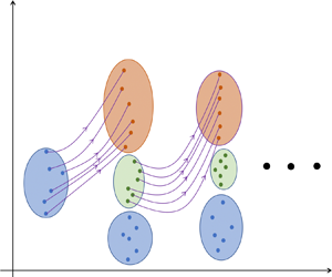
In this study, we use HOS as the nonlinear phase-resolved wave model, coupled with the EnKF for DA. Figure 1 shows a schematic illustration of the proposed EnKF–HOS coupled framework. At initial time  $t=t_0$, measurements
  $\eta _{{m},0}(\boldsymbol {x})$ and
  $\psi _{{m},0}(\boldsymbol {x})$ are available, according to which we generate ensembles of perturbed measurements,
  $\eta _{{m},0}^{(n)}(\boldsymbol {x})$ and
  $\psi _{{m},0}^{(n)}(\boldsymbol {x})$,
  $n=1,2,\ldots ,N$, with
  $N$ the ensemble size, following the known measurement error statistics (see details in § 2.3). A forecast step is then performed, in which an ensemble of
  $N$ HOS simulations are conducted, taking
  $\eta _{{m},0}^{(n)}(\boldsymbol {x})$ and
  $\psi _{{m},0}^{(n)}(\boldsymbol {x})$ as initial conditions for each ensemble member
  $n$ (§ 2.4), until
  $t=t_1$ when the next measurements become available. At
  $t=t_1$, an analysis step is performed where the model forecasts
  $\eta _{{f},1}^{(n)}(\boldsymbol {x})$ and
  $\psi _{{f},1}^{(n)}(\boldsymbol {x})$ are combined with new perturbed measurements
  $\eta _{{m},1}^{(n)}(\boldsymbol {x})$ and
  $\psi _{{m},1}^{(n)}(\boldsymbol {x})$ to generate the analysis results
  $\eta _{{a},1}^{(n)}(\boldsymbol {x})$ and
  $\psi _{{a},1}^{(n)}(\boldsymbol {x})$ (§ 2.5). The analysis step ensures minimal uncertainty represented by the analysis ensembles (figure 1), which is mathematically accomplished through the EnKF algorithm. A new ensemble of HOS simulations are then performed taking
  $\eta _{{a},1}^{(n)}(\boldsymbol {x})$ and
  $\psi _{{a},1}^{(n)}(\boldsymbol {x})$ as initial conditions, and the procedures are repeated for
  $t=t_2, t_3, \ldots$ until the desired forecast time
  $t_{{max}}$ is reached. The details of each step are introduced next in the aforementioned sections, with the addition of an inflation/localization algorithm to improve the robustness of EnKF included in § 2.6, and treatment of the mismatch between predictable zone and measurement region by modifying the EnKF analysis equation in § 2.7. The full process is finally summarized in § 2.8 with algorithm 1.

Figure 1. Schematic illustration of the EnKF–HOS coupled framework. The size of ellipse represents the amount of uncertainty. We use short notations  $[\eta ,\psi ]^{(n)}_{*,j}$ to represent
  $\eta ^{(n)}_{*,j}(\boldsymbol {x}), \psi ^{(n)}_{*,j}(\boldsymbol {x})$ with
  $*={m},{f},{a}$ for measurement, forecast and analysis, and
  $j=0,1,2$.
2.3. Generation of the ensemble of perturbed measurements
As described in § 2.2, ensembles of perturbed measurements are needed at  $t=t_j$, as the initial conditions of
  $N$ HOS simulations for
  $j=0$, and the input of the analysis step for
  $j\geq 1$. As shown in Burgers, Jan van Leeuwen & Evensen (Reference Burgers, Jan van Leeuwen and Evensen1998), using an ensemble of measurements (instead of a single measurement) in the analysis step is essential to obtain the correct ensemble variance of the analysis result. We collect and denote these ensembles by
 \begin{equation}
\boldsymbol{\mathsf{S}}_{{m},j}=\left[\boldsymbol{s}_{{m},j}^{(1)},\boldsymbol{s}_{{m},j}^{(2)},\ldots
\boldsymbol{s}_{{m},j}^{(n)},\ldots \boldsymbol{s}_{{m},j}^{(N-1)},\boldsymbol{s}_{{m},j}^{(N)}\right]
\in \mathbb{R}^{d_j \times N}, \end{equation}
\begin{equation}
\boldsymbol{\mathsf{S}}_{{m},j}=\left[\boldsymbol{s}_{{m},j}^{(1)},\boldsymbol{s}_{{m},j}^{(2)},\ldots
\boldsymbol{s}_{{m},j}^{(n)},\ldots \boldsymbol{s}_{{m},j}^{(N-1)},\boldsymbol{s}_{{m},j}^{(N)}\right]
\in \mathbb{R}^{d_j \times N}, \end{equation}
where  $\boldsymbol{s}$ represents the state variables of surface elevation
  $\eta$ or surface potential
  $\psi$, and
  $\boldsymbol{\mathsf{S}}$ the corresponding ensemble. This simplified notation will be used hereafter when necessary to avoid writing two separate equations for
  $\eta$ and
  $\psi$.
  $\boldsymbol{s}_{{m},j}^{(n)}$ with
  $n=1,2,\ldots ,N$ is the
  $n$th member of the perturbed measurements. Here
  $d_j$ denotes the number of elements in the measurement state vector of either
  $\eta$ or
  $\psi$ at
  $t=t_j$. Without loss of generality, in this work, we use constant
  $d_j=d$ for
  $j \geq 1$, and choose
  $d_0$ for the convenience of specifying the model initial condition (see details in § 3).
To generate each ensemble member  $\boldsymbol{s}_{{m},j}^{(n)}$ from measurements
  $\boldsymbol{s}_{{m},j}$, we first produce
  $\eta _{{m},j}^{(n)}$ from
 \begin{equation} \eta_{{m},j}^{(n)}(\boldsymbol{x})={\eta}_{{m},j}(\boldsymbol{x})+w^{(n)}(\boldsymbol{x}), \end{equation}
where  $w^{(n)}(\boldsymbol {x})$ is the random noise following a zero-mean Gaussian process with spatial correlation function (Evensen Reference Evensen2003, Reference Evensen2009)
 \begin{equation} C(w^{(n)}(\boldsymbol{x}_1),w^{(n)}(\boldsymbol{x}_2))= \begin{cases}c\exp\left(-\displaystyle\frac{|\boldsymbol{x}_1-\boldsymbol{x}_2|^2}{a^2}\right), & \text{for } |\boldsymbol{x}_1-\boldsymbol{x}_2|\leq\sqrt{3}a,\\ 0, & \text{for } |\boldsymbol{x}_1-\boldsymbol{x}_2|>\sqrt{3}a. \end{cases} \end{equation}
In (2.3),  $c$ is the variance of
  $w^{(n)}(\boldsymbol {x})$ and
  $a$ the decorrelation length scale, both of which practically depend on the characteristics of the measurement devices (and thus assumed known a priori). The perturbed measurement of surface potential
  $\psi _{{m},j}^{(n)}$ is reconstructed from
  $\eta _{{m},j}^{(n)}$ based on the linear wave theory,
 \begin{equation} \psi_{{m},j}^{(n)}(\boldsymbol{x})\sim \int\frac{\textrm{i}\omega(\boldsymbol{k})}{|\boldsymbol{k}|}\tilde{\eta}_{{m},j}^{(n)} (\boldsymbol{k})\exp\left({\textrm{i}\boldsymbol{k}\boldsymbol{\cdot}\boldsymbol{x}}\right)\,\textrm{d}\boldsymbol{k}, \end{equation}
where  $\tilde {\eta }^{(n)}_{{m},j}(\boldsymbol {k})$ denotes the
  $n$th member of perturbed surface elevation in Fourier space, and
  $\omega (\boldsymbol {k})$ is the angular frequency corresponding to the vector wavenumber
  $\boldsymbol {k}$. We use ‘
 $\sim$’ instead of ‘=’ in (2.4) as the sign of the integrand relies on the wave travelling direction (and the complex conjugate relation that has to be satisfied for modes
  $\boldsymbol {k}$ and
  $-\boldsymbol {k}$). We remark that this linear construction of
  $\psi _{{m},j}^{(n)}(\boldsymbol {x})$ is the best available given the current radar technology, since
  $\psi _{{m},j}(\boldsymbol {x})$ is either not directly measured or holds a linear relation with
  $\eta _{{m},j}(\boldsymbol {x})$ (Stredulinsky & Thornhill Reference Stredulinsky and Thornhill2011; Hilmer & Thornhill Reference Hilmer and Thornhill2015; Lyzenga et al. Reference Lyzenga, Nwogu, Beck, O'Brien, Johnson, de Paolo and Terrill2015). The additional error introduced by (2.4), however, can be remedied by the EnKF algorithm as will be shown in § 3.
Although the error statistics of the measurements can be fully determined by (2.3) and (2.4), it is a common practice in EnKF to compute the error covariance matrix directly from the ensemble (2.1) (in order to match the same procedure which has to be used for the forecast ensemble). For this purpose, we define an operator  $\mathfrak {C}$ applied on the ensemble
  $\boldsymbol{\mathsf{S}}$ (such as
  $\boldsymbol{\mathsf{S}}_{{m},j}$) such that
 \begin{equation} \mathfrak{C}(\boldsymbol{\mathsf{S}})=\boldsymbol{\mathsf{S}}'(\boldsymbol{\mathsf{S}}')^{\textrm{T}}, \end{equation}
where
 \begin{gather} \boldsymbol{\mathsf{S}}'=\frac{1}{\sqrt{N-1}}\left[\boldsymbol{s}^{(1)}-\bar{\boldsymbol{s}}, \boldsymbol{s}^{(2)}-\bar{\boldsymbol{s}}, \ldots, \boldsymbol{s}^{(n)} -\bar{\boldsymbol{s}},\ldots, \boldsymbol{s}^{(N-1)}-\bar{\boldsymbol{s}},\boldsymbol{s}^{(N)}-\bar{\boldsymbol{s}}\right], \end{gather}
 \begin{gather} \bar{\boldsymbol{s}}=\frac{1}{N}\sum_{n=1}^{N} \boldsymbol{s}^{(n)}. \end{gather}
Therefore, applying  $\mathfrak {C}$ on
  $\boldsymbol{\mathsf{S}}_{{m},j}$,
 \begin{equation} \boldsymbol{\mathsf{R}}_{s,j}=\mathfrak{C}(\boldsymbol{\mathsf{S}}_{{m},j}) \end{equation}
gives the error covariance matrix of the measurements.
2.4. Nonlinear wave model by HOS
Given the initial condition  $\boldsymbol{s}_{{m},j}^{(n)}$ for each ensemble member
  $n$, the evolution of
  $\boldsymbol{s}^{(n)}({\boldsymbol {x}},t)$ is solved by integrating the surface wave equations in Zakharov form (Zakharov Reference Zakharov1968), formulated as
 \begin{gather} \frac{\partial\eta(\boldsymbol{x},t)}{\partial t} + \frac{\partial\psi(\boldsymbol{x},t)}{\partial \boldsymbol{x}} \boldsymbol{\cdot} \frac{\partial\eta(\boldsymbol{x},t)}{\partial \boldsymbol{x}} -\left[1+\frac{\partial\eta(\boldsymbol{x},t)}{\partial \boldsymbol{x}}\boldsymbol{\cdot} \frac{\partial\eta(\boldsymbol{x},t)}{\partial \boldsymbol{x}}\right]\phi_z(\boldsymbol{x},t)=0, \end{gather}
 \begin{gather} \frac{\partial\psi(\boldsymbol{x},t)}{\partial t} + \frac{1}{2}\frac{\partial\psi(\boldsymbol{x},t)}{\partial \boldsymbol{x}}\boldsymbol{\cdot}\frac{\partial\psi(\boldsymbol{x},t)}{\partial \boldsymbol{x}}+\eta(\boldsymbol{x},t)-\frac{1}{2}\left[1+\frac{\partial\eta(\boldsymbol{x},t)}{\partial \boldsymbol{x}}\boldsymbol{\cdot} \frac{\partial\eta(\boldsymbol{x},t)}{\partial \boldsymbol{x}}\right]\phi_z(\boldsymbol{x},t)^2=0, \end{gather}
where  $\phi _z(\boldsymbol {x},t)\equiv \partial \phi /\partial z|_{z=\eta }(\boldsymbol {x},t)$ is the surface vertical velocity with
  $\phi (\boldsymbol {x},z,t)$ being the velocity potential of the flow field, and
  $\psi (\boldsymbol {x},t)=\phi (\boldsymbol {x},\eta ,t)$. In (2.9) and (2.10), we have assumed, for simplicity, that the time and mass units are chosen so that the gravitational acceleration and fluid density are unity (e.g. Dommermuth & Yue Reference Dommermuth and Yue1987).
The key procedure in HOS is to solve for  $\phi _z(\boldsymbol {x},t)$ given
  $\psi (\boldsymbol {x},t)$ and
  $\eta (\boldsymbol {x},t)$, formulated as a boundary value problem for
  $\phi (\boldsymbol {x},z,t)$. This is achieved through a pseudo-spectral method in combination with a mode-coupling approach, with details included in multiple papers such as Dommermuth & Yue (Reference Dommermuth and Yue1987) and Pan, Liu & Yue (Reference Pan, Liu and Yue2018).
2.5. DA scheme by EnKF
Equations (2.9) and (2.10) are integrated in time for each ensemble member to provide the ensemble of forecasts at  $t=t_j$ (for
  $j\geq 1$):
 \begin{equation} \boldsymbol{\mathsf{S}}_{{f},j}=\left[\boldsymbol{s}_{{f},j}^{(1)},\boldsymbol{s}_{{f},j}^{(2)},\ldots \boldsymbol{s}_{{f},j}^{(n)},\ldots \boldsymbol{s}_{{f},j}^{(N-1)},\boldsymbol{s}_{{f},j}^{(N)}\right]\in \mathbb{R}^{L \times N}, \end{equation}
where  $L$ is the number of elements in the forecast state vector and
  $\boldsymbol{s}_{{f},j}^{(n)}(\boldsymbol {x})\equiv \boldsymbol{s}_{{f}}^{(n)}(\boldsymbol {x},t_j)$ is the
  $n$th member of the ensembles of model forecast results. The error covariance matrix of the model forecast can be computed by applying the operator
  $\mathfrak {C}$ on
  $\boldsymbol{\mathsf{S}}_{{f},j}$:
 \begin{equation} \boldsymbol{\mathsf{Q}}_{s,j}=\mathfrak{C}(\boldsymbol{\mathsf{S}}_{{f},j}). \end{equation}
An analysis step is then performed, which combines the ensembles of model forecasts and perturbed measurements to produce the optimal analysis results (Carrassi et al. Reference Carrassi, Bocquet, Bertino and Evensen2018):
 \begin{equation}
\mathop{\boldsymbol{\mathsf{S}}_{{a},j}}_{L \times
N}=\mathop{\boldsymbol{\mathsf{S}}_{{f},j}}_{L \times
N}+\mathop{\boldsymbol{\mathsf{K}}_{s,j}}_{L\times
d}[\mathop{\boldsymbol{\mathsf{S}}_{{m},j}}_{d\times
N}-\mathop{\boldsymbol{\mathsf{G}}_j}_{d\times L}
\mathop{\boldsymbol{\mathsf{S}}_{{f},j}}_{L\times N}],
\end{equation}
\begin{equation}
\mathop{\boldsymbol{\mathsf{S}}_{{a},j}}_{L \times
N}=\mathop{\boldsymbol{\mathsf{S}}_{{f},j}}_{L \times
N}+\mathop{\boldsymbol{\mathsf{K}}_{s,j}}_{L\times
d}[\mathop{\boldsymbol{\mathsf{S}}_{{m},j}}_{d\times
N}-\mathop{\boldsymbol{\mathsf{G}}_j}_{d\times L}
\mathop{\boldsymbol{\mathsf{S}}_{{f},j}}_{L\times N}],
\end{equation}
where
 \begin{equation}
{\boldsymbol{\mathsf{K}}_{s,j}}={\boldsymbol{\mathsf{Q}}_{s,j}}{\boldsymbol{\mathsf{G}}_j^{\textrm{T}}}\left[\boldsymbol{\mathsf{G}}_j\boldsymbol{\mathsf{Q}}_{s,j}\boldsymbol{\mathsf{G}}_j^{\textrm{T}}+\boldsymbol{\mathsf{R}}_{s,j}\right]^{{-}1}
\end{equation}
\begin{equation}
{\boldsymbol{\mathsf{K}}_{s,j}}={\boldsymbol{\mathsf{Q}}_{s,j}}{\boldsymbol{\mathsf{G}}_j^{\textrm{T}}}\left[\boldsymbol{\mathsf{G}}_j\boldsymbol{\mathsf{Q}}_{s,j}\boldsymbol{\mathsf{G}}_j^{\textrm{T}}+\boldsymbol{\mathsf{R}}_{s,j}\right]^{{-}1}
\end{equation}
is the optimal Kalman gain matrix of the state (for  $\boldsymbol{s}=\eta$ or
  $\boldsymbol{s}=\psi$). Here
  $\boldsymbol{\mathsf{G}}_j$ is a linear operator, which maps a state vector from the model space to the measurement space:
  $\mathbb {R}^L\to \mathbb {R}^{d}$. In the present study,
  $\boldsymbol{\mathsf{G}}_j$ is constructed by considering a linear interpolation (or Fourier interpolation (Grafakos Reference Grafakos2008)) from the space of model forecast, i.e.
  $\boldsymbol{s}_{{f},j}^{(n)}$, to the space of measurements, i.e.
  $\boldsymbol{s}_{{m},j}^{(n)}$.
While we have now completed the formal introduction of the EnKF–HOS algorithm (and all steps associated with figure 1), additional procedures are needed to improve the robustness of EnKF and address the possible mismatch between the predictable zone and measurement region. These will be discussed, respectively, in §§ 2.6 and 2.7, with the former leading to a (heuristic but effective) correction of  $\boldsymbol{\mathsf{S}}_{{f},j}$ and
  $\boldsymbol{\mathsf{Q}}_{s,j}$ before (2.13) and (2.14) are applied, and the latter a modification of (2.13) when the mismatch occurs.
2.6. Adaptive inflation and localization
With  $N\rightarrow \infty$ and exact representation of physics by (2.9) and (2.10), it is expected that (2.11) and (2.12) capture the accurate statistics of the model states and (2.13) provides the true optimal analysis. However, due to the finite ensemble size and the underrepresented physics in (2.9) and (2.10), errors associated with statistics computed by (2.12) may lead to suboptimal analysis and even (classical) filter divergence (Evensen Reference Evensen2003, Reference Evensen2009; Carrassi et al. Reference Carrassi, Bocquet, Bertino and Evensen2018). These errors have been investigated by numerous previous studies (Hansen Reference Hansen2002; Evensen Reference Evensen2003; Lorenc Reference Lorenc2003; Hamill & Whitaker Reference Hamill and Whitaker2005; Houtekamer et al. Reference Houtekamer, Mitchell, Pellerin, Buehner, Charron, Spacek and Hansen2005; Evensen Reference Evensen2009; Carrassi et al. Reference Carrassi, Bocquet, Bertino and Evensen2018), which are characterized by (i) underestimates of the ensemble variance in
  $\boldsymbol{\mathsf{Q}}_{s,j}$ and (ii) spurious correlations in
  $\boldsymbol{\mathsf{Q}}_{s,j}$ over long spatial distances. To remedy this situation, adaptive inflation and localization (respectively, for error (i) and (ii)) are usually applied as common practices in EnKF to correct
  $\boldsymbol{\mathsf{S}}_{{f},j}$ and
  $\boldsymbol{\mathsf{Q}}_{s,j}$ before they are used in (2.13) and (2.14).
In this work, we apply the adaptive inflation algorithm (Anderson & Anderson Reference Anderson and Anderson1999; Anderson Reference Anderson2007) in our EnKF–HOS framework. Specifically, each ensemble member in (2.11) is linearly inflated before the subsequent computation, i.e.
 \begin{equation}
\boldsymbol{s}^{(n),{inf}}_{{f},j}=\sqrt{\lambda_j}(\boldsymbol{s}^{(n)}_{{f},j}-\bar{\boldsymbol{s}}_{{f},j})
+\bar{\boldsymbol{s}}_{{f},j},\quad n=1,2,\ldots,N,\end{equation}
\begin{equation}
\boldsymbol{s}^{(n),{inf}}_{{f},j}=\sqrt{\lambda_j}(\boldsymbol{s}^{(n)}_{{f},j}-\bar{\boldsymbol{s}}_{{f},j})
+\bar{\boldsymbol{s}}_{{f},j},\quad n=1,2,\ldots,N,\end{equation}
where  $\lambda _j\geq 1$ is referred to as the covariance inflation factor. The purpose of (2.15) is to amplify the underestimated ensemble variance in
  $\boldsymbol{\mathsf{Q}}_{s,j}$, especially when
  $\bar {\boldsymbol{s}}_{{f},j}$ is far from
  $\boldsymbol{s}_{{m},j}$, therefore, to avoid ignorance of
  $\boldsymbol{\mathsf{S}}_{{m},j}$ in (2.13) (i.e. filter divergence) due to the overconfidence in the forecast. The appropriate value of
  $\lambda _j$ can be determined at each
  $t=t_j$ through the adaptive inflation algorithm (Anderson Reference Anderson2007), which considers
  $\lambda _j$ as an additional state variable maximizing a posterior distribution
  $p(\lambda _j|\eta _{{m},j})$. The detailed algorithm is presented in Appendix A.
After obtaining the inflated  $\boldsymbol{\mathsf{Q}}_{s,j}$, a localization scheme is applied, which removes the spurious correlation by performing the Schur product (i.e. element-wise matrix product) between
  $\boldsymbol{\mathsf{Q}}_{s,j}$ and a local-correlation function
  $\boldsymbol {\mu }$ (Carrassi et al. Reference Carrassi, Bocquet, Bertino and Evensen2018),
 \begin{equation} \boldsymbol{\mathsf{Q}}^{loc}_{s,j}=\boldsymbol{\mu}\circ\boldsymbol{\mathsf{Q}}_{s,j}, \end{equation}
with  $\boldsymbol {\mu }$ defined as the Gaspari–Cohn function (see Appendix B for details).
2.7. Interplay between predictable zone and measurement region
The predictable zone is a spatiotemporal zone where the wave field is computationally tractable given an observation of the field in a limited space at a specific time instant (Naaijen, Trulsen & Blondel-Couprie Reference Naaijen, Trulsen and Blondel-Couprie2014; Köllisch et al. Reference Köllisch, Behrendt, Klein and Hoffmann2018; Qi et al. Reference Qi, Wu, Liu and Yue2018b). Depending on the wave travelling direction, the boundary of the spatial predictable zone moves in time with speed  $c_{{g}}^{{max}}$ or
  $c_{{g}}^{{min}}$, which are the maximum and minimum group speeds within all wave modes of interest (see figure 2 for an example of predictable zone
  $\mathcal {P}(t)$ and unpredictable zone
  $\mathcal {U}(t)$ for a unidirectional wave field starting with initial data in
  $[0,X]$).

Figure 2. The spatial–temporal predictable zone (red) for a case of unidirectional waves which are assumed to travel from left to right, with initial data in  $[0,X]$ at
  $t=t_{j-1}$. The boundary of the computational domain is indicated by the purple vertical lines. The left and right boundary moves with speed
  $c_{{g}}^{{max}}$ and
  $c_{{g}}^{{min}}$, respectively. At
  $t=t_j$, the spatial predictable zone
  $\mathcal {P}_j$ (yellow) is located in
  $[x_c,x_r]=[c_{{g}}^{{max}}(t_j-t_{j-1}), X+c_{{g}}^{{min}}(t_j-t_{j-1})]$ (or in
  $[x_c, X]$ within the computational domain), and the unpredictable zone
  $\mathcal {U}_j$ (orange) is located in
  $[0,x_c]$.
In practice, for a forecast from  $t_{j-1}$ to
  $t_j$, the predictable zone
  $\mathcal {P}(t)$ at
  $t=t_j$ only constitutes a subregion of the computational domain (see caption of figure 2), and there is no guarantee that the measurement region
  $\mathcal {M}_j$ overlaps with the predictable zone
  $\mathcal {P}_j=\mathcal {P}(t_j)$. This requires a special treatment of the region where the measurements are available but the forecast is untrustworthy, i.e.
  $\boldsymbol {x}\in (\mathcal {U}_j\cap \mathcal {M}_j)$, where
  $\mathcal {U}_j=\mathcal {U}(t_j)$. To address this issue, we develop a modified analysis equation which replaces (2.13) when considering the interplay between
  $\mathcal {P}_j$,
  $\mathcal {U}_j$ and
  $\mathcal {M}_j$.
We consider our computational region as a subset of  $\mathcal {P}_j\cup \mathcal {M}_j$, so that the analysis results at all
  $\boldsymbol {x}$ can be determined from the prediction and/or measurements. We further partition the forecast and analysis state vectors
  $\boldsymbol{s}_{{f},j}^{(n)}$ and
  $\boldsymbol{s}_{{a},j}^{(n)}$ (in the computational domain), as well as the measurement state vector
  $\boldsymbol{s}_{{m},j}^{(n)}$ (in
  $\mathcal {M}_j$), according to
 \begin{equation}
\boldsymbol{\mathsf{S}}_{*,j}\in\mathbb{R}^{L\times N} =
\begin{bmatrix}
\boldsymbol{\mathsf{S}}^{\mathcal{P}}_{*,j}\in\mathbb{R}^{L^{\mathcal{P}}\times
N}\\
\boldsymbol{\mathsf{S}}^{\mathcal{U}}_{*,j}\in\mathbb{R}^{L^{\mathcal{U}}\times
N} \end{bmatrix} ,\quad
\boldsymbol{\mathsf{S}}_{m,j}\in\mathbb{R}^{d\times N} =
\begin{bmatrix}
\boldsymbol{\mathsf{S}}^{\mathcal{P}}_{m,j}\in\mathbb{R}^{d^{\mathcal{P}}\times
N}\\
\boldsymbol{\mathsf{S}}^{\mathcal{U}}_{m,j}\in\mathbb{R}^{d^{\mathcal{U}}\times
N} \end{bmatrix},
\end{equation}
\begin{equation}
\boldsymbol{\mathsf{S}}_{*,j}\in\mathbb{R}^{L\times N} =
\begin{bmatrix}
\boldsymbol{\mathsf{S}}^{\mathcal{P}}_{*,j}\in\mathbb{R}^{L^{\mathcal{P}}\times
N}\\
\boldsymbol{\mathsf{S}}^{\mathcal{U}}_{*,j}\in\mathbb{R}^{L^{\mathcal{U}}\times
N} \end{bmatrix} ,\quad
\boldsymbol{\mathsf{S}}_{m,j}\in\mathbb{R}^{d\times N} =
\begin{bmatrix}
\boldsymbol{\mathsf{S}}^{\mathcal{P}}_{m,j}\in\mathbb{R}^{d^{\mathcal{P}}\times
N}\\
\boldsymbol{\mathsf{S}}^{\mathcal{U}}_{m,j}\in\mathbb{R}^{d^{\mathcal{U}}\times
N} \end{bmatrix},
\end{equation}
where  $*={f},{a}$. The variables with superscript
  $\mathcal {U}$ (
 $\mathcal {P}$) represent the part of state vectors for which
  $\boldsymbol {x}\in \mathcal {U}_j$ (
 $\boldsymbol {x}\in \mathcal {P}_j$), with associated number of elements
  $L^{\mathcal {U}}$ and
  $d^{\mathcal {U}}$ (
 $L^{\mathcal {P}}$ and
  $d^{\mathcal {P}}$) for
  $\boldsymbol{s}_{*,j}^{(n)}$ and
  $\boldsymbol{s}_{{m},j}^{(n)}$. The modified analysis equation is formulated as
 \begin{gather}
\mathop{\boldsymbol{\mathsf{S}}^{\mathcal{P}}_{{a},j}}_{L^\mathcal{P}\times
N}=\mathop{\boldsymbol{\mathsf{S}}^{\mathcal{P}}_{{f},j}}_{L^\mathcal{P}\times
N}+\mathop{\boldsymbol{\mathsf{K}}^{\mathcal{P}}_{s,j}}_{L^\mathcal{P}\times
d^\mathcal{P}}[\mathop{\boldsymbol{\mathsf{S}}^{\mathcal{P}}_{{m},j}}_{d^\mathcal{P}\times
N}-\mathop{\boldsymbol{\mathsf{G}}^{\mathcal{P}}_j}_{d^\mathcal{P}\times
L^\mathcal{P}}
\mathop{\boldsymbol{\mathsf{S}}^{\mathcal{P}}_{{f},j}}_{L^\mathcal{P}\times N}], \end{gather}
\begin{gather}
\mathop{\boldsymbol{\mathsf{S}}^{\mathcal{P}}_{{a},j}}_{L^\mathcal{P}\times
N}=\mathop{\boldsymbol{\mathsf{S}}^{\mathcal{P}}_{{f},j}}_{L^\mathcal{P}\times
N}+\mathop{\boldsymbol{\mathsf{K}}^{\mathcal{P}}_{s,j}}_{L^\mathcal{P}\times
d^\mathcal{P}}[\mathop{\boldsymbol{\mathsf{S}}^{\mathcal{P}}_{{m},j}}_{d^\mathcal{P}\times
N}-\mathop{\boldsymbol{\mathsf{G}}^{\mathcal{P}}_j}_{d^\mathcal{P}\times
L^\mathcal{P}}
\mathop{\boldsymbol{\mathsf{S}}^{\mathcal{P}}_{{f},j}}_{L^\mathcal{P}\times N}], \end{gather}
 \begin{gather}
\mathop{\boldsymbol{\mathsf{S}}^{\mathcal{U}}_{{a},j}}_{L^\mathcal{U}\times
N}=\mathop{\boldsymbol{\mathsf{H}}_j}_{L^{\mathcal{U}}\times
d}\mathop{\boldsymbol{\mathsf{S}}_{{m},j}}_{d\times N},
\end{gather}
\begin{gather}
\mathop{\boldsymbol{\mathsf{S}}^{\mathcal{U}}_{{a},j}}_{L^\mathcal{U}\times
N}=\mathop{\boldsymbol{\mathsf{H}}_j}_{L^{\mathcal{U}}\times
d}\mathop{\boldsymbol{\mathsf{S}}_{{m},j}}_{d\times N},
\end{gather}
where  $\boldsymbol{\mathsf{K}}^{\mathcal {P}}_{s,j}= \boldsymbol{\mathsf{K}}_{s,j}(1:L^{\mathcal {P}},1:d^{\mathcal {P}})$ and
  $\boldsymbol{\mathsf{G}}^{\mathcal {P}}_{s,j}= \boldsymbol{\mathsf{G}}_{s,j}(1:d^{\mathcal {P}},1:L^{\mathcal {P}})$ are submatrices of
  $\boldsymbol{\mathsf{K}}_{s,j}$ and
  $\boldsymbol{\mathsf{G}}_{s,j}$ associated with
  $\boldsymbol {x}\in \mathcal {P}_j$ in both measurement and forecast (analysis) spaces,
  $\boldsymbol{\mathsf{H}}_j$ is a linear operator which maps a state vector from measurement space to unpredictable zone in the analysis space:
  $\mathbb {R}^d\to \mathbb {R}^{L^\mathcal {U}}$ (based on linear/Fourier interpolation).
By implementing (2.18a),  $\boldsymbol{\mathsf{S}}^{\mathcal {U}}_{{f},j}$ is discarded in the analysis to compute
  $\boldsymbol{\mathsf{S}}^{\mathcal {P}}_{{a},j}$; and by (2.18b),
  $\boldsymbol{\mathsf{S}}^{\mathcal {U}}_{{a},j}$ is determined only from the measurements
  $\boldsymbol{\mathsf{S}}_{{m},j}$ without involving
  $\boldsymbol{\mathsf{S}}^{\mathcal {U}}_{{f},j}$. Therefore, the modified EnKF analysis equation provides the minimum analysis error when considering the interplay among
  $\mathcal {P}_j$,
  $\mathcal {U}_j$ and
  $\mathcal {M}_j$.
2.8. Pseudocode and computational cost
Finally, we provide a pseudocode for the complete EnKF–HOS coupled algorithm in algorithm 1. For an ensemble forecast by HOS, the algorithm takes  $O(NLlogL)$ operations for each time step
  $\Delta t$. For the analysis step at
  $t= t_j$, the algorithm has a computational complexity of
  $O(dLN)$ for (2.13) and
  $O(dL^2)+O(d^3)+O(d^2L)$ for (2.14) (if Gaussian elimination is used for the inverse). Therefore, the average computational complexity for one time step is
  $O(NLlogL)+O(dL^2)/(\tau /\Delta t)$ (for
  $L>\sim N$ and
  $L>\sim d$), with
  $\tau$ the DA interval.
Algorithm 1 Algorithm for the EnKF–HOS method.

3. Numerical results
To test the performance of the EnKF–HOS algorithm, we apply it on a series of cases with both synthetic and real ocean wave fields. For the former, we use a reference HOS simulation to generate the true wave field, on top of which we superpose random errors to generate the synthetic noisy measurements. For the latter, we use real data collected by a shipborne Doppler coherent marine radar (Nwogu & Lyzenga Reference Nwogu and Lyzenga2010; Lyzenga et al. Reference Lyzenga, Nwogu, Beck, O'Brien, Johnson, de Paolo and Terrill2015). The adaptive inflation and localization algorithms are only applied for the latter case, where the under-represented physics in (2.9) and (2.10) significantly influences the model statistics. The perturbed measurement ensemble (2.1) are generated with parameters  $c=0.0025 \sigma ^2_{\eta }$ (where
  $\sigma _{\eta }$ is the standard deviation of the surface elevation field) and
  $a=\lambda _0/8$ (where
  $\lambda _0$ is the fundamental wavelength in the computational domain) in (2.3) in all cases unless otherwise specified. We remark that these choices may not reflect the true error statistics of the radar measurement, which unfortunately has not been characterized yet. In all HOS computations, we use a nonlinearity order
  $M=4$ to solve (2.9) and (2.10) considering sufficiently deep water. The results from EnKF–HOS simulations are compared with HOS-only simulations (both taking noisy measurements as initial conditions) to demonstrate the advantage of the new EnKF–HOS method.
3.1. Synthetic cases
We consider the synthetic cases where the true solution of a wave field ( $\eta ^{{true}}(\boldsymbol {x},t)$ and
  $\psi ^{{true}}(\boldsymbol {x},t)$) is generated by a single reference HOS simulation starting from the (exact) initial condition. The (noisy) measurements of surface elevation are generated by superposing random error on the true solution,
 \begin{equation} \eta_{{m},j}(\boldsymbol{x})=\eta^{true}(\boldsymbol{x},t_j)+v(\boldsymbol{x}),\quad j=0,1,2\ldots, \end{equation}
where  $v(\boldsymbol {x})$ is a random field, which represents the measurement error and shares the same distribution as
  $w^{(n)}$ (see (2.2) and (2.3)). For simplicity in generating the initial model ensemble, we use
  $\eta _{{m},0}\in \mathbb {R}^L$ in (3.1) (i.e.
  $d_0=L$ in (2.1)), and
  $\eta _{{m},j}\in \mathbb {R}^d$ for
  $j\geq 1$ with
  $d$ specified in each case below. Similar to
  $\psi ^{(n)}_{{m},j}(\boldsymbol {x})$,
  $\psi _{{m},0}(\boldsymbol {x})$ is generated based on the linear wave theory,
 \begin{equation} \psi_{{m},0}(\boldsymbol{x})\sim \int\frac{\textrm{i}\omega(\boldsymbol{k})}{|\boldsymbol{k}|}\tilde{\eta}_{{m},0}(\boldsymbol{k}) \exp\left({\textrm{i}\boldsymbol{k}\boldsymbol{\cdot}\boldsymbol{x}}\right)\,\textrm{d}\boldsymbol{k}, \end{equation}
where  $\tilde {\eta }_{{m},0}(\boldsymbol {k})$ denotes the measurement of surface elevation in Fourier space at
  $t=0$. Although the linear relation (3.2) may introduce initial error in
  $\psi _{{m},0}(\boldsymbol {x})$, the EnKF algorithm ensures the sequential reduction of the error with the increase of time.
Depending on how the true solution is generated, we further classify the synthetic cases into idealistic and realistic cases. In the idealistic case, the true solution is taken from an HOS simulation with periodic boundary conditions, so that the entire computational domain is predictable. In the realistic case, we consider the true solution as a patch in the boundless ocean (practically taken from a patch in a much larger domain where the HOS simulation is conducted), and the interplay between  $\mathcal {M}_j$ and
  $\mathcal {P}_j$ discussed in § 2.7 is critical. Correspondingly, we apply the modified EnKF analysis equation (2.18) only in the realistic cases.
To quantify the performance of EnKF–HOS and HOS-only methods, we define an error metric
 \begin{equation} \epsilon(t;\mathcal{A})=\frac{\displaystyle\int_\mathcal{A}\mid\eta^{true}(\boldsymbol{x},t)-\eta^{{sim}}(\boldsymbol{x},t)\mid^2 d\mathcal{A}}{2\sigma_{\eta}^2 \mathcal{A}}, \end{equation}
where  $\mathcal {A}$ is a region of interest based on which the spatial average is performed (here we use
  $\mathcal {A}$ to represent both the region and its area),
  $\eta ^{{sim}}(\boldsymbol {x},t)$ represents the simulation results obtained from EnKF–HOS (the ensemble average in this case) or the HOS-only method, and
  $\sigma _\eta$ is the standard deviation of, say,
  $\eta ^{{true}}$ in
  $\mathcal {A}$. It can be shown that the definition (3.3) yields
  $\epsilon (t;\mathcal {A})=1-\rho _{\mathcal {A}}(\eta ^{true},\eta ^{sim})$, with
 \begin{equation} \rho_{\mathcal{A}}(\eta^{a},\eta^{b})=\frac{\displaystyle\int_\mathcal{A}\eta^{a}(\boldsymbol{x},t) \eta^{b}(\boldsymbol{x},t) d\mathcal{A}}{\sigma_{\eta}^2 \mathcal{A}}, \end{equation}
being the correlation coefficient between  $\eta ^{a}$ and
  $\eta ^{b}$ (in this case
  $\eta ^{{true}}$ and
  $\eta ^{sim}$). Therefore,
  $\epsilon (t;\mathcal {A})=1$ corresponds to the case that all phase information is lost in the simulation.
In the following, we show results for idealistic and realistic cases of synthetic irregular wave fields. Preliminary results validating the EnKF–HOS method for Stokes waves in the idealistic setting can be found in Wang & Pan (Reference Wang and Pan2020).
3.1.1. Results for idealistic cases
We consider idealistic cases with both 2-D (with one horizontal direction  $x$) and three-dimensional (3-D) (with two horizontal directions
  $\boldsymbol {x}=(x,y)$) wave fields. The true solutions for both situations are obtained from reference simulations starting from initial conditions prescribed by a realization of the JONSWAP spectrum
  $S(\omega )$, with a spreading function
  $D(\theta )$ for the 3-D case (where
  $\omega$ and
  $\theta$ are the angular frequency and angle with respect to the positive
  $x$ direction).
For the 2-D wave field, we use an initial spectrum  $S(\omega )$ with global steepness
  $k_pH_s/2=0.11$, peak wavenumber
  $k_p=16k_0$ with
  $k_0$ the fundamental wavenumber in the computational domain and enhancement factor
  $\gamma =3.3$. In the (reference, EnKF–HOS and HOS-only) simulations,
  $L=256$ grid points are used in spatial domain
  $[0,2{\rm \pi} )$. The noisy measurements
  $\boldsymbol{s}_{{m},j}$ are generated through (3.1) and (3.2), with a comparison between
  $\boldsymbol{s}_{{m},0}(x)$ and
  $\boldsymbol{s}^{{true}}(x,t_0)$ shown in figure 3.

Figure 3. Plots of (a)  $\eta ^{{true}}(x,t_0)$ (—–) and
  $\eta _{{m},0}(x)$ (– – –, red); (b)
  $\psi ^{{true}}(x,t_0)$ (—–) and
  $\psi _{{m},0}(x)$ (– – –, red).
Both EnKF–HOS and HOS-only simulations start from initial measurements  $s_{{m},0}(x)$. In the EnKF–HOS method, the ensemble size is set to be
  $N=100$, and measurements at
  $d=2$ locations of
  $x/(2{\rm \pi} )=100/256$ and
  $170/256$ are assimilated into the model (assuming from measurements of two buoys) with a constant DA interval
  $\tau =t_j-t_{j-1}=T_p/16$, where
  $T_p=2{\rm \pi} /\sqrt {k_p}$ from the dispersion relation.
The error  $\epsilon (t;\mathcal {A})$ with
  $\mathcal {A}=[0,2{\rm \pi} )$ obtained from EnKF–HOS and HOS-only simulations are shown in figure 4. For the HOS-only method, i.e. without DA,
  $\epsilon (t;\mathcal {A})$ increases in time from the initial value
  $\epsilon (0;\mathcal {A})\approx 0.05$, and reaches
  $O(1)$ at
  $t/T_p\approx 100$. In contrast,
  $\epsilon (t;\mathcal {A})$ from the EnKF–HOS simulation keeps decreasing, and becomes several orders of magnitude smaller than that from the HOS-only method (and two orders of magnitude smaller than the measurement error) at the end of the simulation. For visualization of the wave fields, figure 5 shows snapshots of
  $\eta ^{{true}}(x)$ and
  $\eta ^{{sim}}(x)$ (with EnKF–HOS and HOS-only methods) at three time instants of
  $t/T_p=5, 45\ \text {and}\ 95$, which indicates the much better agreement with
  $\eta ^{{true}}(x)$ when DA is applied. Notably, at and after
  $t/T_p=45$, the EnKF–HOS solution is not visually distinguishable from
  $\eta ^{true}(x)$.

Figure 4. Error  $\epsilon (t;\mathcal {A})$ with
  $\mathcal {A}=[0,2{\rm \pi} )$ from EnKF–HOS (– – –, red) and HOS-only (—–) methods, for the 2-D idealistic case.

Figure 5. Surface elevations  $\eta ^{{true}}(x)$ (
 $\circ$, blue),
  $\eta ^{{sim}}(x)$ with EnKF–HOS (– – –, red) and HOS-only (—–) methods, at (a)
  $t/T_p=5$, (b)
  $t/T_p=50$ and (c)
  $t/T_p=95$.
The influence of the parameter  $c$ (reflecting the measurement error) on the results from both methods are summarized in table 1. We present the critical time instants
  $t^*$ when
  $\epsilon (t^*;\mathcal {A})$ reaches
  $O(1)$ in the HOS-only method, i.e. when the simulation completely loses the phase information. As expected, all cases lose phase information for sufficiently long time, and the critical time
  $t^*$ decreases with the increase of
  $c$. In contrast, for EnKF–HOS method, the error
  $\epsilon (t;\mathcal {A})$ decreases with time and reaches
  $O(10^{-3})$ at
  $t=100T_p$ in all cases.
Table 1. Values of  $t^*$ in HOS-only method and
  $\epsilon (100T_p;\mathcal {A})$ in EnKF–HOS method for different values of
  $c$.
$c$.

We further investigate the effects of EnKF parameters on the performance, including DA interval  $\tau$, the ensemble size
  $N$ and the number of DA locations
  $d$. The errors
  $\epsilon (t;\mathcal {A})$ obtained with different parameter values are plotted in figure 6 (for
  $\tau$ from
  $T_p/16$ to
  $T_p/2$), figure 7 (for
  $N$ from 40 to 100) and figure 8 (for
  $d$ from 1 to 4). In the tested ranges, the performance of EnKF–HOS is generally better (i.e. faster decrease of
  $\epsilon (t;\mathcal {A})$ with an increase of
  $t$) for smaller
  $\tau$, larger
  $N$ and larger
  $d$. In addition, for
  $\tau =T_p/2$ as shown in figure 6,
  $\epsilon (t;\mathcal {A})$ slowly increases with time, indicating a situation that the assimilated data is not sufficient to counteract the deviation of HOS simulation from the true solution (due to the chaotic nature of (2.9) and (2.10)). It is also found that when
  $N=20$, the error increases with time, mainly due to the filter divergence caused by insufficient ensemble size to capture the error statistics.

Figure 6. Error  $\epsilon (t;\mathcal {A})$ with
  $\mathcal {A}=[0,2{\rm \pi} )$ from EnKF–HOS method for
  $\tau =T_p/16$ (– – –, red),
  $\tau =T_p/8$ (
 $\Box$, brown),
  $\tau =T_p/4$ (
 $\circ$, magenta) and
  $\tau =T_p/2$ (—–, blue). Other parameter values are kept the same as the main 2-D idealistic case.

Figure 7. Error  $\epsilon (t;\mathcal {A})$ with
  $\mathcal {A}=[0,2{\rm \pi} )$ from EnKF–HOS method for
  $N=20$ (
 $\Box$),
  $N=40$ (—–, brown),
  $N=70$ (
 $\circ$, blue) and
  $N=100$ (– – –, red). Other parameter values are kept the same as the main 2-D idealistic case.

Figure 8. Error  $\epsilon (t;\mathcal {A})$ with
  $\mathcal {A}=[0,2{\rm \pi} )$ from EnKF–HOS method for
  $d=1$ at
  $x/(2{\rm \pi} )=100/256$ (—–, magenta),
  $d=2$ at
  $x/(2{\rm \pi} )=100/256 \text { and }170/256$ (– – –, red) and
  $d=4$ at
  $x/(2{\rm \pi} )=100/256, 135/256, 170/256 \text { and }205/256$ (
 $\circ$, blue). Other parameter values are kept the same as the main 2-D idealistic case.
Finally, we compare the EnKF–HOS algorithm with the explicit Kalman filter method developed by Yoon et al. (Reference Yoon, Kim and Choi2015), where the evolution of the wave field is solved by (2.9) and (2.10) while the propagation of the covariance matrix is linearized. To manifest the contrast between the two approaches, we use as an initial condition a JONSWAP spectrum with a greater global steepness  $k_pH_s/2=0.15$, yet keeping all other parameters the same as the main 2-D idealistic case. Figure 9 compares the errors
  $\epsilon (t;\mathcal {A})$ with
  $\mathcal {A}=[0,2{\rm \pi} )$ from the EnKF–HOS method and the explicit Kalman filter method. Although both errors decrease with time, the EnKF–HOS method shows a faster decreasing rate, with
  $\epsilon (100T_P;\mathcal {A})$ approximately one order of magnitude smaller than that from the explicit Kalman filter method.

Figure 9. Error  $\epsilon (t;\mathcal {A})$ with
  $\mathcal {A}=[0,2{\rm \pi} )$ from EnKF–HOS method (– – –, red) and the explicit Kalman filter method by Yoon et al. (Reference Yoon, Kim and Choi2015) (—–, blue).
For the 3-D wave field, we use the same initial spectrum  $S(\omega )$ as in the main 2-D idealistic case, with a direction spreading function
 \begin{equation} D(\theta)= \begin{cases} \displaystyle\frac{2}{\beta}\cos^2\left(\displaystyle\frac{\rm \pi}{\beta}\theta\right), & \text{for }\displaystyle-\frac{\beta}{2}<\theta<\displaystyle\frac{\beta}{2},\\ 0, & \text{otherwise}, \end{cases} \end{equation}
where  $\beta ={\rm \pi} /6$ is the spreading angle. The (reference, EnKF–HOS and HOS-only) simulations are conducted with
  $L=64\times 64$ grid points. In the EnKF–HOS method,
  $N=100$ ensemble members are used, and data from
  $d=10$ locations (randomly selected with uniform distribution) are assimilated with interval
  $\tau =T_p/16$.
Figure 10 shows the error  $\epsilon (t;\mathcal {A})$ (with
  $\mathcal {A}=[0,2{\rm \pi} )\times [0,2{\rm \pi} )$) obtained from the EnKF–HOS and HOS-only methods. Similar to the 2-D case, we see that
  $\epsilon (t;\mathcal {A})$ from the EnKF–HOS method decreases with time, and becomes several orders of magnitude smaller than that from the HOS-only method (with the latter increasing with time). A closer scrutiny for error on a snapshot can be obtained by defining a local spatial error at a time instant
  $t$:
$t$:
 \begin{equation} e(\boldsymbol{x};t)=\frac{\mid\eta^{{true}}(\boldsymbol{x},t) -\eta^{{sim}}(\boldsymbol{x},t)\mid}{\sigma_{\eta}}. \end{equation}
Three snapshots at  $e(\boldsymbol {x};t)$ for
  $t/T_p=5,~50$ and
  $95$ are shown in figure 11, demonstrating the much smaller error achieved using the EnKF–HOS method especially for large
  $t$, i.e. the superior performance of including DA in the simulation.

Figure 10. Error  $\epsilon (t;\mathcal {A})$ with
  $\mathcal {A}=[0,2{\rm \pi} )\times [0,2{\rm \pi} )$ from EnKF–HOS (– – –, red) and HOS-only (—–) methods, for the 3-D idealistic case.

Figure 11. Local spatial error  $e(\boldsymbol {x};t)$ obtained with EnKF–HOS (a,c,e) and HOS-only (b,d,f) methods at (a,b)
  $t/T_p=5$, (c,d)
  $t/T_p=50$ and (e,f)
  $t/T_p=95$ for the 3-D idealistic case.
3.1.2. Results for realistic cases
We consider  $\eta ^{{true}}(\boldsymbol {x})$ for the realistic case taken from a subregion
  $\mathcal {R}$ with quarter edge length of a periodic computational domain
  $\mathcal {W}$, i.e. a patch in the ocean (see figure 12a). The reference simulation in
  $\mathcal {W}$ is performed with
  $256\times 256$ grid points, with all other parameters kept the same as the 3-D idealistic reference simulation. The EnKF–HOS and HOS-only simulations are conducted over
  $\mathcal {R}=[0,2{\rm \pi} )\times [0,2{\rm \pi} )$ with
  $L=64\times 64$ grid points, starting from initial noisy measurements. For
  $j\geq 1$, We further consider a practical situation where the measurements are obtained from a marine radar and only available in
  $\mathcal {M}_j=\mathcal {B}^{{c}}\cap \mathcal {R}$, where
  $\mathcal {B}=\{\boldsymbol {x}|x>{\rm \pi} , {\rm \pi}/2< y<3{\rm \pi} /2\}$ (say a structure of interest located within
  $\mathcal {B}$ preventing the surrounding measurements, see figure 12b). We use
  $d=2176$ (locating on every computational grid point in
  $\mathcal {M}_j$) and an assimilation interval
  $\tau =T_p/4$.

Figure 12. Schematic illustration of spatial domains: (a) periodic computational domain  $\mathcal {W}$ for the reference simulation and subregion
  $\mathcal {R}$ for EnKF–HOS and HOS-only simulations; (b) computational region
  $\mathcal {R}$ with measurement zone
  $\mathcal {M}_j$ marked by blue, region
  $\mathcal {B}=\{\boldsymbol {x}|x>{\rm \pi} , {\rm \pi}/2< y<3{\rm \pi} /2\}$ with no data available by yellow, predictable zone
  $\mathcal {P}_j$ by checker board, and unpredictable zone
  $\mathcal {U}_j$ by downward diagonal stripes.
In this case, the use of modified EnKF analysis (2.18) is critical due to the interplay between  $\mathcal {M}_j$,
  $\mathcal {P}_j$ and
  $\mathcal {U}_j$. In particular, the left, upper/lower bounds of
  $\mathcal {P}(t)$ moves (towards right, down/up), respectively, with speeds
  $c_{g,x}^{{max}}$ and
  $c_{g,y}^{{max}}$, i.e. the maximum group speeds up in the
  $x$ and
  $y$ directions (corresponding to the group speed of mode
  $\boldsymbol {k}=(1,1)$). After applying the modified EnKF analysis equation (2.18), which takes into consideration of
  $\mathcal {M}_j$,
  $\mathcal {P}_j$ and
  $\mathcal {U}_j$ (see a sketch in figure 12b),
  $\mathcal {P}_j$ is recovered to fill in
  $\mathcal {R}$ due to the DA. In contrast, in the HOS-only method,
  $\mathcal {P}(t)\equiv \mathcal {P}^*(t)$ keeps shrinking and vanishes for sufficient time. We consider two error metrics
  $\epsilon (t; \mathcal {R})$ and
  $\epsilon (t; \mathcal {P}^*(t))$, which are plotted in figure 13 for both EnKF–HOS and HOS-only methods. For HOS-only simulation,
  $\epsilon (t; \mathcal {R})$ increases rapidly in time and reaches
  $O(1)$ at
  $t/T_p\sim O(3)$. This is resulted from the chaotic nature of (2.9) and (2.10), as well as the larger error in
  $\mathcal {U}(t)$. For EnKF–HOS simulation,
  $\epsilon (t; \mathcal {R})$ decreases with time and reaches a constant level of
  $O(0.002)$ after
  $t/T_p\sim O(3)$. The further reduction of the error is prohibited due to the region
  $\mathcal {U}(t)$, because
  $\epsilon (t; \mathcal {U}(t))$ has a lower bound from the measurement error. The general trend of
  $\epsilon (t; \mathcal {P}^*(t))$ is similar to
  $\epsilon (t; \mathcal {R})$, but the magnitude of
  $\epsilon (t; \mathcal {P}^*(t))$ is smaller than that of
  $\epsilon (t; \mathcal {R})$ for both methods. In particular, the growth rate of
  $\epsilon (t; \mathcal {P}^*(t))$ for the HOS-only method is comparable to those in 2-D/3-D idealistic cases. This is due to the removal of
  $\mathcal {U}(t)$ from
  $\mathcal {A}$ in the computation of the error.

Figure 13. The error metric  $\epsilon (t; \mathcal {R})$ obtained from EnKF–HOS (
 $\circ$, red) and HOS-only (—–) methods; and
  $\epsilon (t; \mathcal {P}^*(t))$ obtained from EnKF–HOS (
 $\Box$, blue) and HOS-only (– – –, magenta) methods, for the 3-D realistic case.
To further understand the error characteristics, we plot the local spatial error  $e(\boldsymbol {x};t)$ at
  $t/T_p=2.875, 4.875$ and
  $7.25$ for both methods in figure 14. While the spatial error generally increases in time for the HOS-only method,
  $e(\boldsymbol {x};t)$ from the EnKF–HOS method is significantly smaller and exhibits a heterogeneous spatial distribution. Within
  $\mathcal {U}_j$,
  $e(\boldsymbol {x};t)$ is relatively high with the same order of the measurement error. In
  $\mathcal {P}_j$,
  $e(\boldsymbol {x};t)$ decreases with time and becomes significantly lower than that in
  $\mathcal {U}_j$. Remarkably, this also applies to the region where measurements are not available (i.e.
  $\mathcal {M}^c\cap \mathcal {R}$) as the waves in this region travel from upstream locations where DA is performed. This result is of practical importance as it shows that the wave forecast at a location of interest in the ocean (say the location of an offshore structure) can be made accurate through DA in the upstream region.

Figure 14. Local spatial error  $e(\boldsymbol {x};t)$ obtained from (a,c,e) EnKF–HOS and (b,d,f) HOS-only methods for the 3-D realistic case, at (a,b)
  $t/T_p=2.875$, (c,d)
  $t/T_p=4.875$ and (e,f)
  $t/T_p=7.25$. The regions bounded by the black dash lines represent
  $\mathcal {P}^*(t)$ with the HOS-only method.
3.2. Results with real radar measurements
In this section, we test the performance of the EnKF–HOS method with real radar measurements of the ocean wave field. The measurements are obtained from a shipborne X-band ( $9.4\ \text {GHz}$) Doppler coherent marine radar off the coast of Southern California. We consider a patch from the radar-scanned area as our initial domain of interest
  $\mathcal {R}_0$, which covers a
  $480\ \textrm {m}\times 480\ \textrm {m}$ area resolved on a
  $64\times 64$ grid (figure 15). The starting time of computation is
  $2013\text {-}09\text {-}13{T}01:00:13{Z}$, with a global wave steepness
  $k_pH_s/2=0.027$ from the initial radar data. The direction of waves is determined for each mode (travelling at its phase speed) by finding the direction which correlates better with two sequential snapshots of surface elevation (which gives consistent direction for almost all the modes). In both EnKF–HOS and HOS-only simulations, we rescale the computational domain
  $\mathcal {R}_j$ to
  $[0,2{\rm \pi} )\times [0,2{\rm \pi} )$ and use
  $L=64\times 64$ grid points. For EnKF, we use
  $d=64\times 64$, which covers the whole patch, and set the DA interval the same as radar data collection interval, which fluctuates in time around
  $T_p/4=2.82\ \text {s}$. The ensemble size is set to be
  $N=100$. For adaptive inflation, we use
  $\bar {\lambda }_0=1$ in the prior distribution of
  $\lambda _0$ (see Appendix A) to sequentially determine
  $\lambda _j$ in (2.15), which is applied at each
  $t=t_j$ together with the localization (2.16).

Figure 15. Initial surface elevation  $\eta _{m,0}(\boldsymbol {x})/H_s$ (with
  $H_s=1.70\ \text {m}$) measured by radar at
  $t=t_0$, i.e.
  $2013$-
 $09$-
$09$- $13{T}01:00:13{Z}$.
A critical issue in this case is the movement of  $\mathcal {M}_j$ in time due to the ship speed (around
  $0.2\ \textrm {m}\ \textrm {s}^{-1}$), which results in a mismatch between
  $\mathcal {M}_j$ and the computational region
  $\mathcal {R}_{j-1}$ at each
  $t=t_j$. To address this issue, we shift the computational region from
  $\mathcal {R}_{j-1}$ to
  $\mathcal {R}_j$ which matches
  $\mathcal {M}_j$. In the EnKF–HOS method, we further partition
  $\mathcal {R}_j$ into
  $\mathcal {P}_j$ and
  $\mathcal {U}_j$ (using the predictable zone calculated from
  $\mathcal {R}_{j-1}$) and apply the modified analysis equation (2.18) accordingly. In the HOS-only method, we use Fourier periodic extension (Grafakos Reference Grafakos2008) to obtain the wave field covering
  $\mathcal {R}_j$.
Since the true solution is not available in this case, we directly use  $\rho _{\mathcal {A}}(\eta _{{m},j}, \eta ^{{sim}})$ (see (3.4)) as the metric to evaluate the performance. Figure 16 plots
  $\rho _{\mathcal {A}}(\eta _{{m},j}, \eta ^{{sim}})$ with
  $\mathcal {A}=\mathcal {R}_j$ and
  $\mathcal {A}=\mathcal {P}^*(t)$ (for which the shrinking speed is still taken as the group speed of mode
  $\boldsymbol {k}=(1,1)$) obtained from EnKF–HOS and HOS-only methods. While all time series start from
  $1$ at
  $t=t_0$,
  $\rho _{\mathcal {R}_j}(\eta _{{m},j}, \eta ^{{sim}})$ and
  $\rho _{\mathcal {P}^*(t)}(\eta _{{m},j}, \eta ^{{sim}})$ from the HOS-only simulation quickly approach
  $O(0.25)$ and
  $O(0.40)$ within one peak period
  $T_p$, indicating the (almost) complete loss of the phase information. This is much faster than any synthetic case, mainly due to the under-resolved physics in (2.9) and (2.10) with respect to the real ocean (which includes extra physical effects of current, wind, etc.). Furthermore,
  $\rho _{\mathcal {R}_j}(\eta _{{m},j}, \eta ^{{sim}})$ from the HOS-only method is lower in comparison with that reported in Lyzenga et al. (Reference Lyzenga, Nwogu, Beck, O'Brien, Johnson, de Paolo and Terrill2015) (approximately
  $0.5\sim 0.75$ after
  $10T_P$, which we have confirmed using our code). This is mainly due to the different region used in Lyzenga et al. (Reference Lyzenga, Nwogu, Beck, O'Brien, Johnson, de Paolo and Terrill2015), which may feature less significant effects of current and wind, as well as smaller radar error due to its smaller distance from the ship. In contrast to results from the HOS-only method, the correlation
  $\rho _{\mathcal {R}_j}(\eta _{{m},j}, \eta ^{{sim}})$ and
  $\rho _{\mathcal {P}^*(t)}(\eta _{{m},j}, \eta ^{{sim}})$ from EnKF–HOS remain at
  $O(0.75)$ (with the latter slightly greater than the former), retaining the phase information for arbitrarily long time. Figure 17 further plots the snapshots of
  $\eta _{{m},j}(\boldsymbol {x})$ and
  $\eta ^{{sim}}(\boldsymbol {x},t)$ at two cross-sections of
  $y/(2{\rm \pi} )=1/3$ and
  $2/3$ for both methods at three time instants of
  $t/T_p=1, 5$ and
  $9$. It can be visually observed that the EnKF–HOS results are (on average) much closer to
  $\eta _{{m},j}(\boldsymbol {x})$ for all cases.

Figure 16. Time series of  $\rho _{\mathcal {R}_j}(\eta _{{m},j}, \eta ^{{sim}})$ from EnKF–HOS (– – –, red) and HOS-only (—–) methods; and
  $\rho _{\mathcal {P}^*(t)}(\eta _{{m},j}, \eta ^{{sim}})$ from EnKF–HOS (
 $\circ$, blue) and HOS-only (
 $\diamond$, brown) methods.

Figure 17. Snapshots of  $\eta_{{m},j}(\boldsymbol {x})$ (
![]() , blue) and
, blue) and  $\eta^{sim}(\boldsymbol {x},t)$ from EnKF–HOS (– – –, red) and HOS-only (—–) methods, at two cross-sections (a,c,e)
  $y/(2{\rm \pi} )=1/3$ and (b,d,f)
  $y/(2{\rm \pi} )=2/3$, and time instants (a,b)
  $t/T_p=1$,(c,d)
  $t/T_p=5$ and (e,f)
  $t/T_p=9$.
We finally test the effect of parameter  $\bar {\lambda }_0$ on the performance of EnKF–HOS. In general, the value of
  $\bar {\lambda }_0$ can be considered as a control of the extent to which the inflation is applied. For larger values of
  $\bar {\lambda }_0$, it is expected that the ensemble variance of (2.11) is amplified to a greater extent, and more weights are assigned to measurements when the analysis (2.18) is applied. Physically, larger values of
  $\bar {\lambda }_0$ may be chosen if the model is associated with significant under-represented physics (thus severely underestimates the variance in (2.11)). To elucidate this effect of
  $\bar {\lambda }_0$, we test another value of
  $\bar {\lambda }_0=2$, and compare the resulting
  $\rho _{\mathcal {R}_j}(\eta _{{m},j}, \eta ^{{sim}})$ with that from
  $\bar {\lambda }_0=1$ in figure 18. Indeed, the result for
  $\bar {\lambda }_0=2$ shows a higher correlation with the measurement, with
  $\rho _{\mathcal {R}_j}$ above
  $O(0.8)$ for all time. We note that the higher value of
  $\rho _{\mathcal {R}_j}$ does not imply the closeness of
  $\eta ^{{sim}}$ to
  $\eta ^{{true}}$, since the relation between
  $\eta _{{m},j}$ and
  $\eta ^{{true}}$ is not known in this case.

Figure 18. Time series of  $\rho _{\mathcal {R}_j}(\eta _{{m},j}, \eta ^{{sim}})$ with
  $\bar \lambda _0=1.0$ (– – –, red) and
  $\bar \lambda _0=2.0$ (—–, brown).
4. Conclusions
In this paper, we develop the ensemble-based DA capability for phase-resolved wave forecast, resulting in a new EnKF–HOS method. A unique consideration in EnKF–HOS is the treatment of the interplay between predictable and measurement zones, which is successfully accounted for through a modified analysis equation. The performance of the EnKF–HOS method is extensively tested and compared with the (traditional) HOS-only method using both synthetic wave fields and real radar data. In all cases, significant advantages are demonstrated by using the EnKF–HOS method, namely the dramatic reduction of forecast error and retaining the phase information for an arbitrarily long time with DA of radar data. In contrast, the phase information is lost within one peak period in the HOS-only method when considering the real ocean waves. The parameters involved in the EnKF–HOS method are carefully benchmarked, including the ensemble size, DA interval, number of DA locations and the inflation factor. The developed EnKF–HOS algorithm is intrinsically parallel and very suitable for implementation on a graphics processing unit (GPU), a compact device that can be conveniently installed in the offshore environment (our ongoing work). Finally, the accuracy of the EnKF–HOS method can be further improved given deeper knowledge about the radar measurement error, which we recommend as one of the next essential focuses for the remote sensing community.
Acknowledgements
We would like to thank Dr D. Lyzenga, Dr O. Nwogu and Dr R. Beck in the Department of Naval Architecture and Marine Engineering at the University of Michigan, for providing and interpreting the radar data. We also thank Dr P. Hess from the Office of Naval Research to grant us permission to use this data set for research.
Funding
The research is funded by the Michigan Institute for Computational Discovery and Engineering (MICDE) through a 2019 Catalyst Grant. The computational resources are provided by NSF-XSEDE grant TG-CTS200016.
Declaration of interests
The authors report no conflict of interest.
Appendix A. Adaptive inflation
We apply the adaptive inflation algorithm developed by Anderson (Reference Anderson2007) to determine the values of  $\lambda _j$ in (2.15). The algorithm is applied at each
  $t=t_j$ (for
  $j\geq 1$), and we shall drop the subscript
  $j$ on other variables in the following description for simplicity.
The key idea in adaptive inflation is to consider  $\lambda$ as an additional state variable and update its value through Bayes’ theorem given the measurements
 \begin{equation} p\left(\lambda|\eta_{{m}}(\boldsymbol{x})\right)\sim p(\lambda)p(\eta_{{m}}(\boldsymbol{x})|\lambda), \end{equation}
where  $p(\lambda )$ is the (given) prior distribution and
  $p(\eta _{{m}}(\boldsymbol {x})|\lambda )$ is the likelihood function. In principle, our purpose is to find the optimal
  $\lambda$ which maximizes the posterior
  $p(\lambda |\eta _{{m}}(\boldsymbol {x}))=p(\lambda |\eta _{{m}}(1),\ldots ,\eta _{{m}}(d))$. Intuitively, the inflation (2.15) using such an optimal
  $\lambda$ provides sufficient variance of the forecast ensemble to cover the measurements, and thus avoid the overconfidence in the forecast when analysis is performed.
By assuming independent measurement errors, it can be shown that the full Bayes’ problem (A1) is equivalent to the sequential problem (which saves significant computational cost, see Anderson (Reference Anderson2007) for details)
 \begin{gather} p\left(\lambda|\eta_{{m}}(1)\right)=p\left(\eta_{{m}}(1)|\lambda\right) p\left(\lambda\right)/\mathcal{Z}_1, \end{gather}
 \begin{gather} p\left(\lambda|\eta_{{m}}(1),\eta_{{m}}(2),\ldots,\eta_{{m}}(i)\right) =p\left(\eta_{{m}}(i)|\lambda\right)p\left(\lambda|\eta_{{m}}(1),\eta_{{m}}(2),\ldots, \eta_{{m}}(i-1)\right)/\mathcal{Z}_i, \end{gather}
where (A3) is applied sequentially for  $i=2,\ldots ,d$, and
  $\mathcal {Z}_i$ are the normalization factors (which do not play a role in the computation).
In computing (A2) and (A3), we use a Gaussian prior distribution,
 \begin{equation} p(\lambda)=\mathcal{N}(\bar{\lambda}_0,\sigma_0^2), \end{equation}
with mean  $\bar {\lambda }_0$ and variance
  $\sigma ^2_0$ (say
  $\bar {\lambda }_0=1$ and
  $\sigma ^2_0={c\bar {\lambda }_0^2}/{H_s^2}$ at
  $j=1$, with the situation of
  $j>1$ discussed at the end of Appendix A). The key computations in (A2) and (A3) are the likelihood functions
  $p(\eta _{{m}}(i)|\lambda )$ for
  $i=1,2,\ldots ,d$, which will be discussed below.
Given a value of  $\lambda$, a member in the forecast ensemble at measurement location
  $i$ is denoted by
  $[\boldsymbol {G}\eta _{f}^{(n),inf}](i)$ with
  $\eta _{f}^{(n),inf}$ given by (2.15). This ensemble is assumed to have a Gaussian distribution consistent with the EnKF framework, with mean
  $[\boldsymbol {G}\bar {\eta }_{{f}}](i)$ and variance
  $\sigma _f(i)^2=\lambda [\boldsymbol {G}\boldsymbol{\mathsf{Q}}_{\eta }\boldsymbol {G}^{\textrm {T}}](i,i)$ (note that only
  $\sigma _f(i)^2$ is affected by the inflation). Let
  $D=\eta _{m}(i) -[\boldsymbol {G}\bar {\eta }_{{f}}](i)$ be the distance between the mean forecast and measurement at location
  $i$, which is drawn from a zero-mean Gaussian random variable
  $\mathcal {D}$ with variance
  $\theta _i^2=\sigma _f(i)^2+\boldsymbol{\mathsf{R}}_\eta (i,i)$ (here we consider the summation of two independent Gaussian random variables and assume that both the measurement and forecast are unbiased). It follows that
 \begin{equation} p\left(\eta_{m}(i)|\lambda\right)=p\left(\mathcal{D}=D|\lambda\right) =\displaystyle\frac{1}{\sqrt{2{\rm \pi}}\theta_i}\exp\left(\displaystyle\frac{-D^2}{2\theta_i^2}\right). \end{equation}
Therefore, the posterior distribution in each equation of (A2) and (A3) can be formulated as
 \begin{equation} p\left(\lambda|\eta_{m}(1),\ldots,\eta_{m}(i)\right) =\displaystyle\frac{1}{{2{\rm \pi}}\theta_i\sigma_{i-1}}\left.\exp\left(-\displaystyle\frac{D^2}{2\theta_i^2} -\frac{(\lambda-\bar{\lambda}_{i-1})^2}{2\sigma_{i-1}^2}\right)\right/\mathcal{Z}_i. \end{equation}
The formulation (and sequential computation) of (A6) for  $i = 1,2,\ldots ,d$ require each posterior
  $p(\lambda |\eta _{m}(1),\ldots ,\eta _{m}(i))$ in (A2) and (A3) (and thus the prior for the next sequential equation) to be approximated by Gaussian distribution
  $\mathcal {G}(\lambda )\sim \mathcal {N}(\bar {\lambda }_i,\sigma _i^2)$. We follow Anderson (Reference Anderson2007) to set the
  $\bar {\lambda }_i$ as the mode of
  $p(\lambda |\eta _{m}(1),\ldots ,\eta _{m}(i))$, and compute
  $\sigma _i$ by considering
  $\varGamma =p(\bar {\lambda }_i|\eta _{m}(1),\ldots ,\eta _{m}(i))/p(\bar {\lambda }_i+\sigma _i|\eta _{m}(1),\ldots ,\eta _{m}(i))=\mathcal {G}(\bar {\lambda }_i)/\mathcal {G}(\bar {\lambda }_i+\sigma _i)$, i.e. the same decay rate of the distribution, which gives
  $\sigma ^2_i=-(\sigma ^2_{i-1}/2)\ln {\varGamma }$.
Finally, we use  $\lambda =\bar {\lambda }_d$ in (2.15) for inflation at
  $t=t_j$, and set
  $\mathcal {N}(\bar {\lambda }_d,\sigma _d^2)$ computed at time
  $t=t_j$ as the prior
  $p(\lambda )$ at
  $t=t_{j+1}$. The computations of (A2) and (A3) are repeated, which completes the full algorithm to determine
  $\lambda$ by adaptive inflation at each
  $t_j$.
Appendix B. Gaspari–Cohn function
The local-correlation function  $\boldsymbol {\mu }$ in the localization equation (2.16) is defined as the Gaspari–Cohn function (Gaspari & Cohn Reference Gaspari and Cohn1999), given by
 \begin{equation} [\boldsymbol{\mu}]_{ij}=\begin{cases} 1-\frac{5}{3}r^2+\frac{5}{8}r^3+\frac{1}{2}r^4-\frac{1}{4}r^5, & \text{for }0\leq r < 1,\\ 4-5r+\frac{5}{3}r^2+\frac{5}{8}r^3-\frac{1}{2}r^4+\frac{1}{12}r^5-\frac{2}{3r}, & \text{for }1\leq r < 2, \\ 0, & \text{for }r\geq 2, \end{cases} \end{equation}
where  $r=|\boldsymbol {x}_i-\boldsymbol {x}_j|/(\sqrt {3}a/2)$, with
  $a$ taking the same value as in (2.3). A plot of
  $\boldsymbol {\mu }(r)$ is provided in figure 19.

Figure 19. Gaspari–Cohn correlation function  $\boldsymbol {\mu }(r)$ used in the localization.


 Open access