Article

Quantifying Contributions of Local Emissions and Regional Transport to NOX in Beijing Using TROPOMI Constrained WRF-Chem Simulation

1
Key Lab of Environmental Optics & Technology, Anhui Institute of Optics and Fine Mechanics, Chinese Academy of Sciences, Hefei 230031, China
2
Department of Precision Machinery and Precision Instrumentation, University of Science and Technology of China, Hefei 230026, China
3
Department of Geography, Hong Kong Baptist University, Hong Kong 999077, China
4
School of Earth and Space Sciences, University of Science and Technology of China, Hefei 230026, China
5
Institute of Physical Science and Information Technology, Anhui University, Hefei 230601, China
6
Department of Earth System Science, Tsinghua University, Beijing 100084, China
7
School of Environmental Science and Optoelectronic Technology, University of Science and Technology of China, Hefei 230026, China
8
Anhui Province Key Laboratory of Polar Environment and Global Change, University of Science and Technology of China, Hefei 230026, China
9
Center for Excellence in Regional Atmospheric Environment, Institute of Urban Environment, Chinese Academy of Sciences, Xiamen 361021, China
10
Key Laboratory of Precision Scientific Instrumentation of Anhui Higher Education Institutes, University of Science and Technology of China, Hefei 230026, China
*
Author to whom correspondence should be addressed.
Remote Sens. 2021, 13(9), 1798; https://doi.org/10.3390/rs13091798
Submission received: 9 April 2021 / Revised: 29 April 2021 / Accepted: 1 May 2021 / Published: 5 May 2021

Abstract

:
Air quality is strongly influenced by both local emissions and regional transport. Atmospheric chemical transport models can distinguish between emissions and regional transport sources in air pollutant concentrations. However, quantifying model inventories is challenging due to emission changes caused by the recent strict control measures taken by the Chinese government. In this study, we use NO2 column observations from the Tropospheric Monitoring Instrument to retrieve top-down nitrogen oxide (NOX) emissions and quantify the contributions of local emissions and regional transport to NOx in Beijing (BJ), from 1 November 2018 to 28 February 2019 (W_2018) and 1 November 2019 to 29 February 2020 (W_2019). In W_2018 and W_2019, the BJ bottom-up NOX emissions from the multi-resolution emission inventory for China in 2017 were overestimated by 11.8% and 40.5%, respectively, and the input of NOX from other cities to BJ was overestimated by 10.9% and 51.6%, respectively. The simulation using our adjusted inventory exhibited a much higher spatial agreement (slope = 1.0, R2 = 0.79) and reduced a mean relative error by 45% compared to those of bottom-up NOX emissions. The top-down inventory indicated that (1) city boundary transport contributes approximately 40% of the NOX concentration in BJ; (2) in W_2019, NOX emissions and transport in BJ decreased by 20.4% and 17.2%, respectively, compared to those of W_2018; (3) in W_2019, NOX influx substantially decreased (−699 g/s) in BJ compared to that of W_2018 despite negative meteorological conditions that should have increased NOx influx by +503 g/s. Overall, the contribution of intercity input to NOx in BJ has declined with decreasing emissions in the surrounding cities due to regional cooperative control measures, and the role of local emissions in BJ NOx levels was more prominent. Our findings indicate that local emissions may play vital roles in regional center city air quality.

Graphical Abstract

1. Introduction

In the past decade, haze in China has been frequently reported at unprecedented PM2.5 concentrations during the autumn and winter, particularly in the North China Plain (NCP). Nitrogen oxides (NOX; NO + NO2), which are primarily discharged by anthropogenic activities, such as fossil fuel combustion [1], are a group of reactive trace gases. NOx is not only toxic to human health, but also play a key role in the formation of secondary aerosol and tropospheric ozone [2]. Therefore, NOx is crucial atmospheric air pollutants.
A series of strict emissions reduction measures was implemented in China beginning in September 2013 [3]. In the past seven years, substantial manpower and material resources have been invested to improve air quality, and major measures have been taken for the atmosphere and ecosystem. To evaluate the effectiveness of air pollution control measures, an accurate and high spatiotemporal resolution of NO2 distribution must be obtained [4,5,6]. Most previous studies have primarily used satellite observations, regional air quality model simulations, or ground-based observations to obtain the trace gas distribution [7,8,9,10,11]. Compared with these methods, the NO2 concentration produced by models (Global 3-D model of atmospheric chemistry driven by meteorological input from the Goddard Earth Observing System (GEOS-Chem) [12], Community Multiscale Air Quality (CMAQ) model, Comprehensive Air Quality Model with Extensions (CAMx)) exhibits a higher spatiotemporal resolution in both the horizontal and vertical directions. Thus, timely NOX emission data are necessary.
A top-down inversion using satellite retrieval products of tropospheric vertical column densities (VCDs) of NO2 is widely used to estimate NOX emissions. This method accounts for the nonlinear effects of horizontal transport, chemical loss, and deposition. Previous studies have estimated NOX emissions from various regions worldwide, including North America, Asia, the Middle East, and Europe [13,14,15,16,17]. This inversion has also been used to produce and validate NOX emission estimations from sources such as soil, lightning, power plants, aircraft, marine vessels, and urban centers [8,18,19,20,21].
The NOX concentration distribution is not only related to regional NOX emissions but also linked with the regional transport of NOX. Several quantitative and qualitative approaches have been applied to evaluate the regional transport of emissions and its effect on local air quality [22,23,24,25]. The backward trajectory based on meteorology analysis has been used to qualitatively identify and describe the major transport direction and pathway of a target city [23,26,27,28]. Additionally, certain studies have used meteorological models or have combined meteorology and air quality observations to determine the relative importance of different source regions as a semi-qualitative assessment. Such studies include footprint analysis [29,30], the potential source contribution function analysis [31,32,33], and flux calculation [34]. Recently, regional transport studies have mostly been based on the chemical transport model [35] to sufficiently consider both the physical and chemical processes. For example, [36] found three primary transport pathways inside the Beijing–Tianjin–Hebei (BTH) region, i.e., the southwest, southeast, and anticlockwise pathway, with the Community Multiscale Air Quality and Integrated Source Apportionment Model (CMAQ-ISAM) [37] quantified the contribution of pollutant transport via PM2.5 concentrations in 13 cities in the BTH region using the CMAQ-ISAM model. These findings have noted the necessity of a regional joint-control strategy. However, these studies are based on inventories relying on indirect information that is often outdated or incomplete, which is insufficient to support the development of a comprehensive joint-control strategy.
Herein, we combined the Tropospheric Monitoring Instrument (TROPOMI) observations and Weather Research and Forecasting with coupled chemistry (WRF-Chem) simulations to obtain accurate NOX emissions for the NCP region (covering 33° N–43° N, 109° E–123° E). We then identify the sources and sinks of NOX in NCP based on the regional transport flux. Finally, we quantify the contributions of NOX local emissions and regional transport to NOX concentrations, distinguishing the roles of meteorology and emissions to the city-boundary transport flux, thus helping the government implement emissions reduction policies at the city level. The remainder of this paper is organized as follows. Section 2 provides detailed information about the model configuration, TROPOMI NO2 retrieval, top-down NOX emissions inversion, and transport flux calculation. The top-down NOX inventory evaluation, relative contribution of NOX emissions and transport flux to NOX concentration, and role of emissions control and meteorology analysis are presented in Section 3. Section 4 presents the discussion. Finally, conclusions are present in Section 5.

2. Materials and Methods

2.1. Model Description and Configuration

The meteorological parameters and NOX concentration were provided by WRF-Chem version 4.0. This modeling system runs in two parts: the dynamic and chemical modules. The WRF model, which is a mesoscale numerical weather prediction system designed for meteorological research and numerical weather forecasting, is used as the dynamic module. A detailed description of the WRF model is available at the WRF website (http://www.wrf-model.org/index.php, last access: 15 March 2020). In addition to dynamical calculations, the chemical module is fully coupled with the WRF model online [38]. A detailed illustration of the chemical composition is provided by Grell et al. [39]. In this work, the simulation domain covered East China and its surrounding area, with a center point of 38.0°N, 115.6°E. The model’s horizontal resolution was selected to be 20 × 20 km2, with 89 × 79 grids (there are 89 grids in the east-west direction and 79 grids in the north-south direction). From the ground level to the top pressure of 10 hPa, there were 44 vertical sigma layers for all grids. The initial meteorological fields and boundary conditions were from the 6-h final operational global analysis (FNL) data. The data were provided by the National Centers for Environmental Prediction (NCEP), and it exhibited a 1° × 1° spatial resolution. Furthermore, the NCEP Administrative Data Processing (ADP) Global Surface Observational Weather Data (ds461.0) and Upper Air Observational Weather Data (ds351.0) with 6-hourly temporal resolution were used to accurately reproduce the meteorology. The physical and chemical parameterization schemes adopted in this study are detailed in Table 1. Further configuration options of the model can be found in our previous study [40]. Table 2 demonstrates that the simulated wind fields are reproducible in comparison with those of the National Office for Oceanic and Atmospheric Administration (NOAA) observations (https://www.ncdc.noaa.gov/, last access: 25 June 2020).
The Carbon-Bond Mechanism version Z photochemical mechanism combined with the Model for Simulating Aerosol Interactions and Chemistry was used to simulate the chemical process in the atmosphere. The anthropogenic emissions were taken from the multi-resolution emission inventory for China in 2017 (MEIC-2017; http://www.meicmodel.org/, last access: 17 March 2020) [41,42]. The biogenic emissions were calculated online using the Model of Emissions of Gases and Aerosols from Nature embedded in the WRF-Chem model. The near-real-time fire emissions from the fire inventory of NCAR based on Moderate Resolution Imaging Spectroradiometer rapid response fire counts (https://www.acom.ucar.edu/acresp/forecast/fire-emissions.shtml, last access: 18 March 2020).

2.2. TROPOMI Satellite Observation

TROPOMI is a passive trace gas spectrometer aboard the Sentinel-5 Precursor satellite, which was launched on 13 October 2017. TROPOMI measures the reflected sunlight of the atmosphere with spectral bands in 270–500 nm (ultraviolet–visible) 675–775 nm (near-infrared), and 2305–2385 nm (short-wave infrared) at a moderate resolution (0.25 nm to 0.6 nm), enabling daily global coverage with a spatial resolution of 7 km × 3.5 km at an exact nadir point [48,49]. In this work, the TROPOMI NO2 product typically followed the satellite trace gas retrieval algorithms by USTC (University of Science and Technology of China) [50]. During NO2 slant column density retrieval, the wavelength range of 405–465 nm was selected for the NO2 spectral fit performed with the QDOAS software package [51]. The QDOAS configurations follow the suggestions in the QA4ECV NO2 project [52]. For NO2 air mass factor (AMF) calculations, the Vector Linearized Discrete Ordinate Radiative-Transfer version 2.7 model [53] was used to calculate the stratospheric and tropospheric NO2 AMF pixel by pixel. During the RTM calculations, a priori NO2 profile with a high-resolution of 20 km × 20 km was taken from the monthly WRF-Chem simulations. Other information, such as cloud top pressure, cloud fraction, and surface albedo, was obtained from the operational TROPOMI cloud dataset [54]. To separate the stratospheric contribution from the total NO2 VCDs, a modified reference sector method, i.e., the STREAM algorithm [55], was applied. For the final tropospheric NO2 VCDs, we utilized a novel P-spline method to re-grid the NO2 VCDs to the Level-3 product at a resolution of 0.2° × 0.2° [56]. TROPOMI data were considered cloud-contaminated and filtered out by the re-gridding algorithm when the cloud radiance fraction was greater than 50% [57,58].

2.3. TROPOMI-Derived Top-Down NOX Emissions

TROPOMI-detected NO2 columns are sensitive to NOX emissions at the surface and are influenced by the NOX lifetime within the plumes. Previous studies [18,59,60] have confirmed that there is a non-linear relationship between changes in surface NOX emissions and changes in tropospheric NO2 columns. This is because an increase in the NOX concentration may promote or inhibit oxidation losses [11]. In the monthly assimilated inversion, we referenced the framework by [61]. The following four steps were followed. (1) Two simulations were performed, one with a priori emissions MEIC-2017 (Emeic) and another with anthropogenic NOX emissions, which increased by 20%. (2) The dimensionless scaling factor β, which reflects the sensitivity of NO2 VCDs to local NOX emissions via NOX-OH chemistry (indicated by Formula (1)), was calculated. (3) Top-down NOX emissions (Etop-down) were estimated with the modeled sensitivity β to scale the a priori emissions (indicated by Equation (2)). (4) The monthly regional NOX distribution was modeled with WRF-chem to combine the top-down emissions.
β = Δ E / E m e i c Δ C / C m e i c
E t o p d o w n = E m e i c ( 1 + β C t r o p o m i C m i e c C m i e c )
where ΔE is the change in anthropogenic NOX emissions in Emeic, which increased by 20%; Cmeic is the simulated NO2 columns with Emeic; ΔC is the change in the monthly average tropospheric-simulated NO2 VCDs after perturbing Emeic anthropogenic NOX emissions by +20%. Ctropomi is the monthly average tropospheric VCDs based on WRF-Chem NO2 vertical profile with Emeic. Equation (2) in this work is a simplified calculation from [61]. In our study, the difference of top-down NOX emissions from Equation (2) is ~0.2% lower than that calculated by [61].

2.4. Horizontal Transportation Flux

To further investigate the source and sink centers of air pollution in the NCP region, the spatial distribution of the transport flux was calculated as follows:
Step 1: Calculate the average wind.
The weight coefficient was derived from the vertical distribution of NO2 under the height of the tropopause layer in each grid. A high NO2 concentration corresponds to a large coefficient. The average wind is equal to the sum of the wind of each layer multiplied by the weight coefficient of the corresponding height.
Step 2: Calculate the horizontal transport flux of grid A (i, j) [62].
East west   direction   f l u x a ( i , j ) = C ( i + 1 , j ) * U ( i + 1 , j ) C ( i 1 , j ) * U ( i , j )
North south   direction   f l u x b ( i , j ) = C ( i , j + 1 ) * V ( i , j + 1 ) C ( i , j 1 ) * V ( i , j )
Horizontal   net   flux   f l u x n e t ( i , j )   =   f l u x a ( i , j )   +   f l u x b ( i , j )
Equations (3) and (4) provide the basic equations to calculate the transport flux of each grid in the region. Where C is the tropospheric NO2 column from the WRF-Chem NO2 simulation. U and V represent the winds in the east–west and north–south directions, respectively. Easterly and northerly are both positive. Equation (5) quantifies the net flux of air pollutants in each grid. A positive net-flux represents the grid outputting NO2 to its surrounding four grids. By contrast, negative values indicate that the four surrounding grids input NO2 into the grid.

2.5. Ancillary Data

In-situ measurements for NO2 analysis were provided by the operational stations of the China Environmental Observation Network operated by the China National Environmental Monitoring Centre (CNEMC; http://www.cnemc.cn/en/, last access: 28 June 2020). The 0–23-h concentrations of these measurements spanning from November 2018 to February 2019 and from November 2019 to February 2020 were used in this study. FNL data were obtained from NCEP FNL Operational Model Global Tropospheric Analyses (https://rda.ucar.edu/datasets/ds083.2/index.html, last access: 15 March 2020). NCAR archive ds351.0 data were downloaded from NCEP ADP Global Upper Air Observational Weather Data Centre (https://rda.ucar.edu/datasets/ds351.0/index.html, last access: 15 March 2020)

3. Results and Discussion

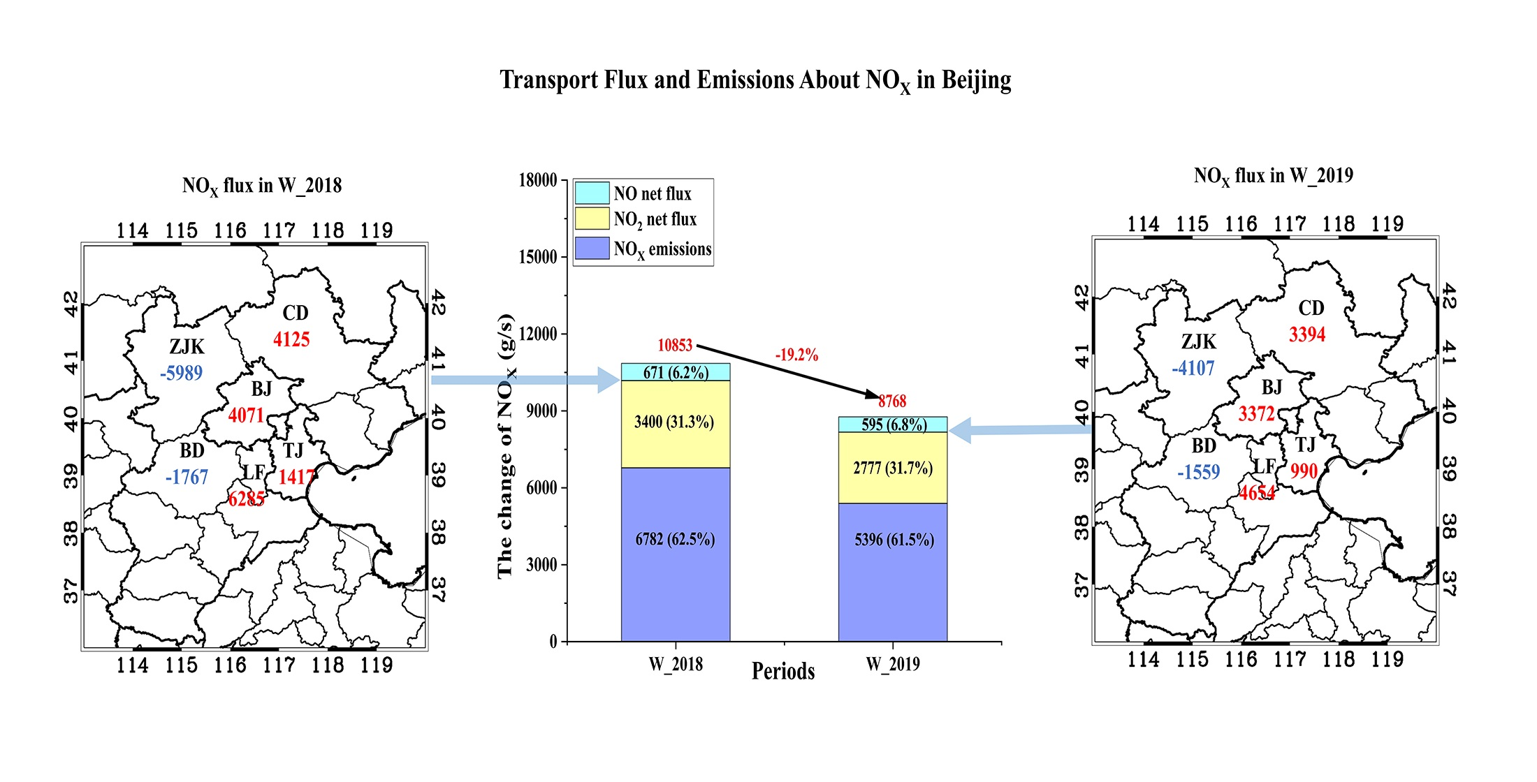
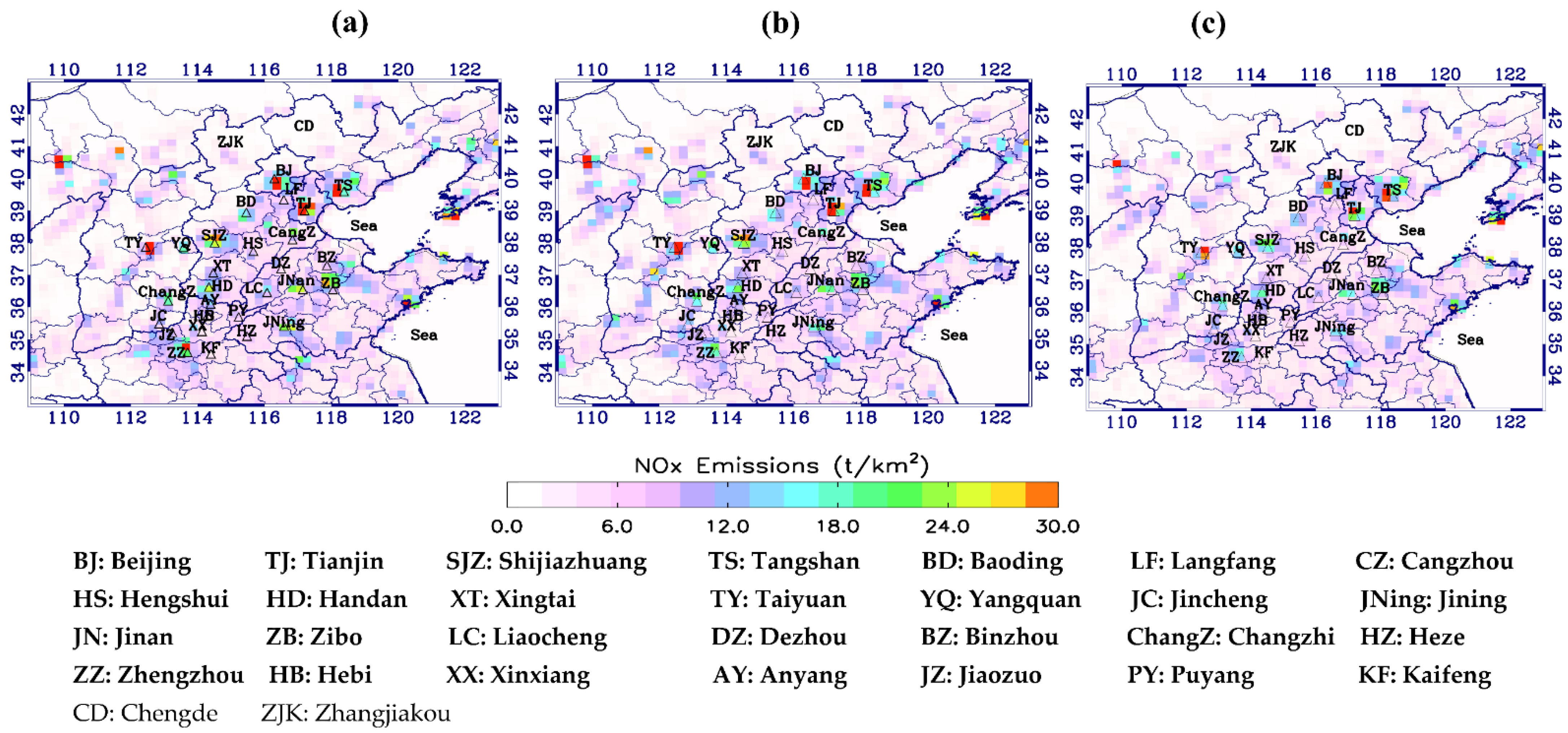
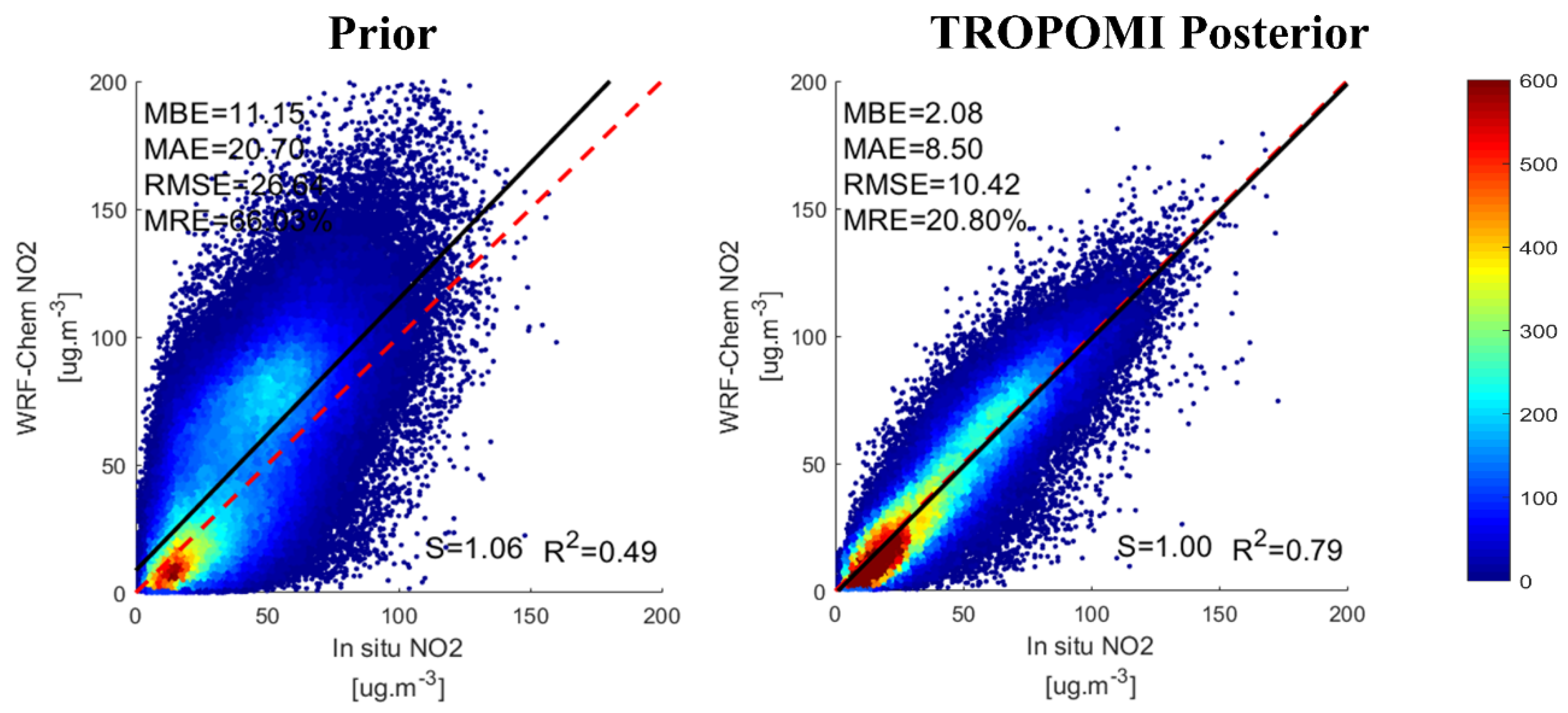
3.1. Top-down Emissions Evaluation

Wintertime air pollution is extremely severe in northern Chinese cities. In February 2017, the Ministry of Environmental Protection in China released the Air Pollution Prevention and Control Work Plan for BTH and its neighboring regions, which referred to the cities that transmit air pollution as “2 + 26” cities (represented by triangles in Figure 1) for the first time. The “2 + 26” cities represent 28 NOX polluted cities in the Beijing-Tianjin-Hebei and surrounding region, including 2 cities with significant NOX pollution (Beijing (BJ) and Tianjin (TJ)) and 26 cities (the rest of the cities) with high NOX concentrations.
Since the implementation of air emissions control in the “2 + 26” cities, the concentration of air pollution has been significantly reduced, and the air quality has been greatly improved. Monthly top-down NOX emissions were derived using the method described in Section 2. Figure 1 displays the spatial distribution of monthly averaged MEIC-2017 and top-down surface NOX emissions. “2 + 26” cities dominated in high NOx emissions. Figure 2 illustrates the regional emission differences. As exhibited in Figure 2a,b, the top-down NOX emissions in the south of BJ, southeast of Hebei province, northwest of Shandong province, and northern of Henan province were significantly reduced by 25–58% when compared to those of MEIC-2017. By contrast, NOX emissions in Taiyuan (TY) and Tangshan (TS) slightly increased. This phenomenon can also be observed in Figure S2a–f, except for January 2020. In February 2020, NO2 VCDs in the south of TY simulated from top-down W_2019 are slightly higher than that simulated from MEIC-2017 (Figure S2h). However, NO2 VCDs in the south of TY simulated from top-down W_2019 is slightly lower than that simulated from top-down W_2018 (Figure S2l) during February 2020. This means that NOx emissions in the south of TY during February 2020 are higher than that in the same period of 2017, but lower than that in the same period of 2019. Figure 2c displays the difference between the top-down inventories in W_2018 and W_2019. NOX emissions in all “2 + 26” cities significantly decreased. The monthly variation analysis (Figure S2i–l) shows that NOX emissions in the south of BJ and southeast of TJ and Langfang (LF) slightly increased, while NOX emissions in the other cities decreased in November 2019 compared to those in November 2018, particularly in central Shanxi. In December 2019, most cities in the southeast of Taihang Mountain exhibited significant NOX emission reductions compared to those in December 2018, while NOX emissions in central Shanxi province and Tangshan increased. In January 2020, NOX emissions across the entire study area exhibited a pronounced decreasing trend compared to those in January 2019; and the NO2 concentration in the BTH demonstrated a reduction of approximately 50% compared with that in January 2019. This result may be attributed to the lockdown policy during the outbreak of the COVID-19 pandemic. Additionally, it may have also resulted from the influence of the Spring Festival holiday.
Figure 3 compares the monthly averaged NO2 tropospheric VCDs simulated from MEIC-2017, top-down NOX emissions, and their differences. Figure 3a illustrates the monthly average distribution of tropospheric NO2 VCDs in W_2018, which was simulated using the MEIC-2017 inventory, and Figure 3b is the same as Figure 3a, except that it uses the top-down W_2018 NOX inventory, which was retrieved from the TROPOMI NO2 concentration during W_2018. Both Figure 3a and Figure 3b exhibit peak NO2 in BJ, TJ, TS, and certain cities in southeast of the Taihang mountains. Figure 3c displays the monthly averaged distribution of tropospheric NO2 in W_2019, which uses the same inventory as that in Figure 3a. The role of meteorological conditions can be understood based on the difference between Figure 3a and Figure 3c. The overall meteorology changes between W_2018 and W_2019 slightly influenced the NO2 VCDs and their spatial distribution. Figure 3d is the same as Figure 3c, except that it uses the top-down W_2018 inventory, the VCD distribution of which is similar to that of Figure 3b. Figure 3e is the same as Figure 3c, except that it uses the top-down W_2019 inventory, which was retrieved from the TROPOMI NO2 observations during W_2019. Figure 3f indicates the difference between Figure 3a and Figure 3b, reflecting the changes in the tropospheric NO2 VCDs during W_2018 when using the calibration inventory compared to that when using MEIC-2017. In most cities, the NO2 concentration dropped significantly, while strong (18–32%) NO2 concentration increases occurred in the center of Shanxi province and TS after NOX emission adjustments during W_2018. In February 2019, the simulated NO2 VCDs using top-down W_2018 inventory was significantly lower than that using MEIC-2017 in the study area (Figure S3a–d,i–l). This result was due to reduced NOX emissions over the Spring Festival holiday. Figure 3g indicates the difference between Figure 3c and Figure 3d, reflecting the changes in the tropospheric NO2 VCDs during W_2019 when using the top-down W_2018 inventory compared to that when using MEIC-2017. The decline in NO2 VCDs in Figure 3g is more pronounced than that in Figure 3f, which was caused by the unfavorable meteorological condition during W_2019 compared to that in W_2018. Figure 3h indicates the differences between Figure 3c and Figure 3e, reflecting the changes in the tropospheric NO2 VCDs during W_2019 when using the calibration inventory compared to that when using MEIC-2017. The NO2 VCDs simulated from the top-down-W_2019 are much lower than those from MEIC-2017, especially in January and February 2020. The NO2 concentration in the BTH region particularly decreased. The decline in NO2 VCDs in Figure 3h is more pronounced than that in Figure 3f, which was caused by the significantly decreased NOX emissions during W_2019. This substantial drop in the NO2 concentration was due to a combination of strict emission controls and the COVID-19 lockdown.
Figure 4 illustrates the simulation with optimized NOX emissions and removing the model’s systematic bias with respect to the hourly surface in-situ NO2 concentration, leading to an improved spatial agreement (slope = 1.0, R2 = 0.79) and reducing the mean relative error by 45%. Our findings demonstrate that air quality model simulations combined with satellite observations can be used to adjust surface NOX emissions before more rigorous bottom-up emissions inventories are released.

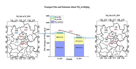
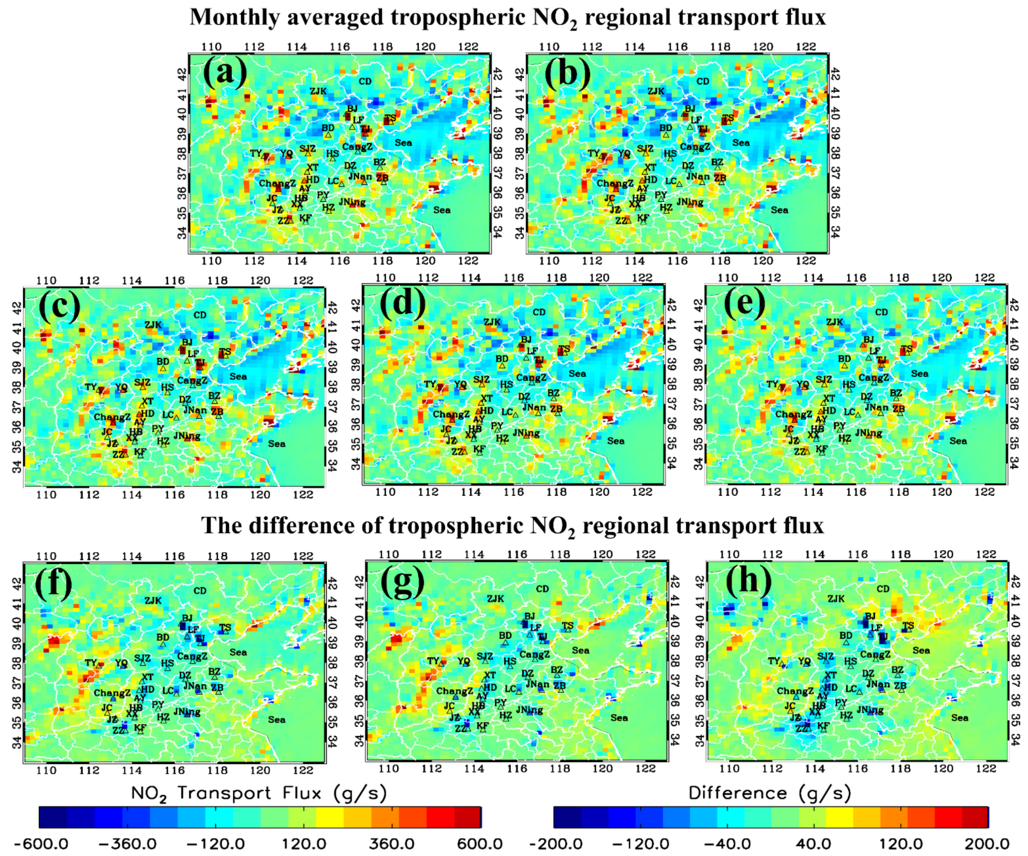
3.2. Regional Transport Flux

Studies have been extensively performed to investigate the impact of regional transport on BJ airborne species [63,64,65]. Figure 5a–h display the NO2 regional transport fluxes and their differences calculated using formulas (3–5), which correspond to Figure 3a–h, respectively. During the two periods, TS, TJ, and cities in southeast of Taihang mountain (Baoding (BD), Shijiazhuang, Xingtai, Handan, Anyang, and Hebi) were significant NO2 sources when using MEIC-2017 (Figure 5a,c), and they were lesser sources when using top-down NOX emissions (Figure 5f–h). These results indicate great achievements in emission reductions due to the implementation of strict emissions control measures. By contrast, cities in central Shanxi province exhibited more NOX emissions when using top-down NOX emissions than when using MEIC-2017 emissions. This result means that TY and its surrounding cities to the north need to strengthen their emission reduction management.
A city that exhibits a high NO2 concentration does not necessarily severely emit NOX. Moreover, the wind field makes NO2 flow into and accumulate in that city, which also leads to heavy NO2 pollution. For example, BJ exhibits a high NO2 concentration during the two periods; however, it is a NOX sink. In addition, the regional distribution of sources and sinks agrees with that of the NOX emissions. Satellite observations can be used to qualitatively analyze source distribution and strength without updating the bottom-up emissions. The distribution of sources in the regional transport flux is affected by the wind field. When the wind speed is low, and the wind direction frequently changes, the transport flux agreement with bottom-up NOX emissions improves. These findings are considerably important for implementing air quality control measures during special events.

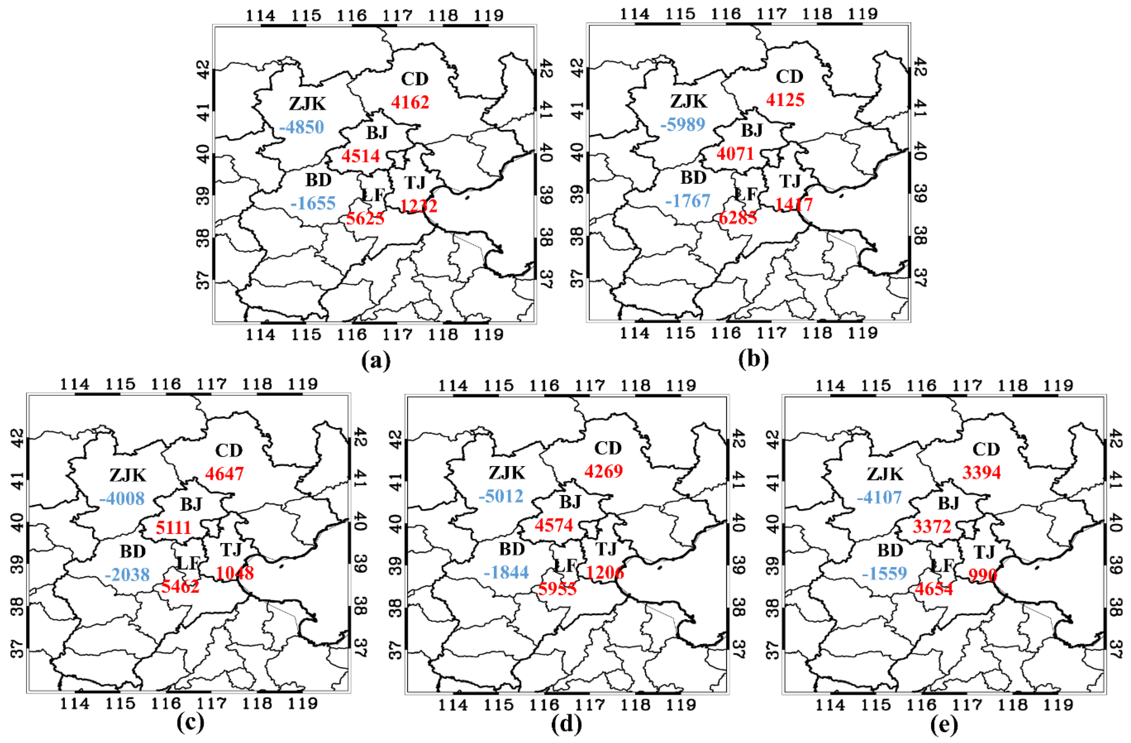
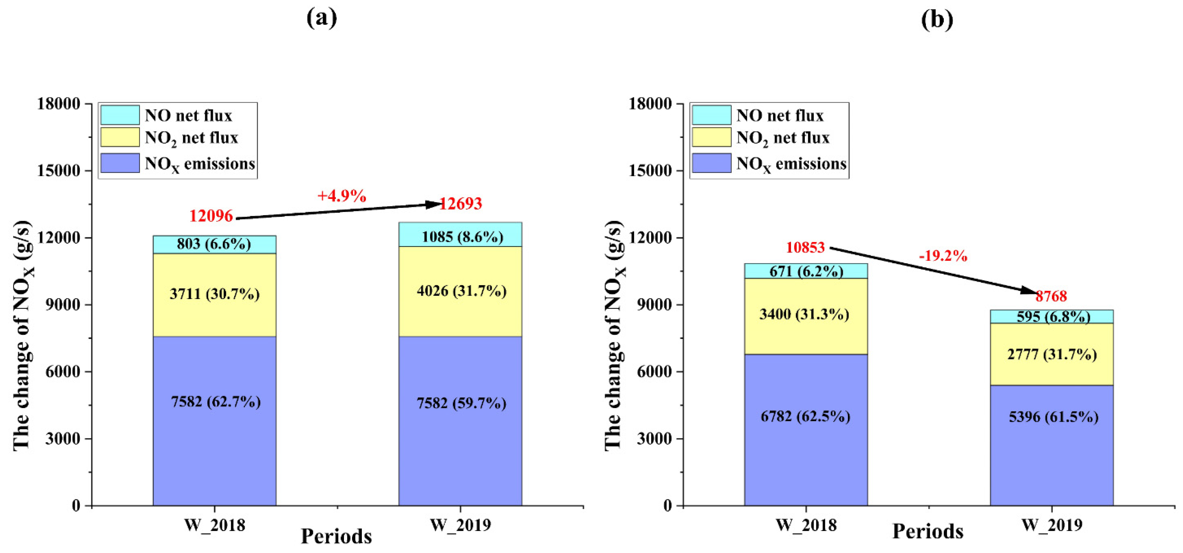
3.3. Assessment of City Boundary Transport Around BJ

To determine the effectiveness of emissions control measures on each city level, the relative contributions of local NOX emissions and city boundary transport fluxes must be quantified. Figure 6 represents the NOX transport fluxes surrounding BJ, the calculation method of which is derived from [35]. BJ is a large NOX sink in both periods. Zhangjiakou (ZJK) and BD, which are upwind of BJ, input NOX into BJ (the NOX transported through the outer boundary is a mixture of different sources and does not solely stem from the neighboring cities). BJ simultaneously exports NOX to the downwind cities, such as Chengde (CD), TJ, and LF. Figure 6a,c demonstrate the transport fluxes between BJ and its surrounding 5 cities during W_2018 and W_2019, which are simulated using MIEC-2017 (same MEIC-2017 NOX emissions but different meteorology). In that case, the difference (Figure 6c minus Figure 6a) in the boundary transport flux of BJ is due to the meteorology change between the two periods. In W_2019, BJ exhibits enhanced NOX input from surrounding cities by 597g/s (13.2%) compared to that of W_2018. The unfavorable meteorology in W_2019 can account for the 13.2% NOX concentration enhancement. Figure 6b exhibits the cities boundary transport flux between BJ and its surrounding cities during W_2018, which is the same as Figure 6a except that it uses the top-down W_2018 inventory. Figure 6d is the same as Figure 6c except that it uses the top-down W_2018 inventory. Comparing Figure 6d and Figure 6b, i.e., the weather of W_2019 compared to that of W_2018, demonstrated an increase in the BJ input flux by 503 g/s (12.4%), which also reflects the adverse meteorological conditions in W_2019 causing NOX concentration enhancement. Figure 6e is the same as Figure 6d, except that the top-down W_2019 inventory was used. Comparing Figure 6e and Figure 6d, the NOX emissions in top-down W_2019 compared to that in the top-down W_2018, for the BJ input were reduced by 1202 g/s (26.3%), which also reflects the favorable emissions control in W_2019 for NOX concentration reduction. Comparing Figure 6b and Figure 6a, the boundary transport flux simulated using MEIC-2017 overestimates the NO2 inflow flux in BJ by 443 g/s (10.9%) during W_2018. Comparing Figure 6e and Figure 6c demonstrates that the boundary transport flux simulated and calculated using MEIC-2017 overestimates the NO2 inflow flux in BJ by 1379 g/s (51.6%) during W_2019. Comparing Figure 6e and Figure 6b reflects that the input of NO2 from cities surrounding BJ exhibits a decrease in NOx emissions of 699 g/s (17.2%) from W_2018 to W_2019. This result is caused by the co-effects of meteorology and emissions changes. The favorable contribution of the emission reduction policy is 26.3%, while the unfavorable contribution of weather is approximately 13%.
Figure 7 displays the NOX emissions and net fluxes of NOX and NO2 from W_2018 to W_2019. As illustrated in Figure 7a, compared with W_2018, BJ NOX emissions remain unchanged (both use MEIC-2017), while NOX input to BJ increased by 13.2% (increase of 597 g/s) due to unfavorable meteorological conditions. BJ total NOX increment (including NOX emissions and NOX net flux) increased by 4.9% during W_2019. After the inventory adjustment, the top-down inventory demonstrates that, in W_2019, NOX emissions and transport in BJ decreased by 20.4% (reduction of 1386 g/s) and 17.2% (reduction of 699 g/s), respectively. BJ total NOX increment decreased by 19.2% compared to that of W_2018 (Figure 7b).
In the two periods, BJ NOX local emissions using MEIC-2017 were overestimated by 11.8% and 40.5%; and the NOX transport flux was underestimated by 10.9% and 51.6%. Based on the top-down inventory, the proportions of emissions in the two winters were 62.5% and 61.5%, and the proportions of the city boundary transport fluxes were 37.5% and 38.5%.

4. Discussion

The assimilation of satellite observations in atmospheric chemical transport models is vital for improving the accuracy of air pollutant simulations. This study derived optimized NOX emissions based on the TROPOMI/WRF-Chem relative difference using a mass balance approach. The pollutant distribution from TROPOMI is significantly impacted by meteorological conditions [66,67,68]. Thereby, the accuracy of this assimilated method (top-down emissions) decreases when strong transport on NO2 occur. The Inversion errors and model-based simulation errors relating local NO2 columns to local emissions constitute the uncertainty of top-down emissions. The overall error of the top-down emissions over NCP areas is estimated at ~50% [16].
Our results have taken COVID-19 lockdown and spring festival into account, which shows dramatic reductions (~50%) in NOX emissions over January 2020. Our results comply with the literature, [69] indicated that concentrations of NO2 decreased by ~45.1% observed by ground-based observations during January 2020 compared with that in January 2019. According to Figure 3, the slope of “Prior” is greater than 1, and the slope of TROPOMI Posterior is equal to 1. It means that the simulated NO2 before assimilation is higher than the observation and more accurate after calibration.
Several studies have found that accurate representation of noonday NO2 columns from highly localized sources requires a high model resolution. Since NOX emissions show a strong variation on the 20 × 20 km2 scale applied in this study. Increasing the model resolution can better represent these local gradients, thus improving the simulation of NO2 concentrations [17,70,71].
The relative proportion of NOX transport in BJ is about 40%. Similar results have been obtained in studies using a comparable regional model [65]. During the Asia-Pacific Economic Cooperation Forum week, non-local emissions contributed to 41.3% of the total PM2.5 concentration in BJ, emphasizing the correctness of strict and synergistic emissions control for BJ and its surrounding provinces.
Future work can be continued on the change of ozone and PM2.5 affected by the NOX emission variety after TROPOMI assimilation.

5. Conclusions

By optimizing NOX emissions with TROPOMI observations, sufficient NO2 simulation performance can be achieved, and the mean relative error can be reduced by 45%. Cities with high NOX emissions exhibit a pronounced decline (by 25–58%) after inventory adjustment. Particularly in January 2020, NOX exhibited a reduction of approximately 50% in BTH compared with that in January 2019. For BJ, in W_2018 and W_2019, the bottom-up NOX emissions were overestimated by 11.8% and 40.5% when compared to the top-down NOX emissions, respectively. According to the top-down inventory, compared with those of W_2018, NOX emissions in BJ decreased by 20.4% during W_2019. A city with decreased NO2 concentration may be due to not only reduced NOX emissions but also lower NO2 inflows. We found that NOX emissions can account for approximately 60% of the NOX concentration, and the remaining 40% is caused by regional transport.
Moreover, by analyzing the regional horizontal transport flux, we can identify the major sources and the strengths of NOX emissions without an immediately updated bottom-up inventory. This approach can be used to evaluate the effectiveness of implementing emission control measures, particularly during special events.
Transport fluxes depend on wind speed and emissions. This NOX inflow and outflow fluxes can be calculated according to the city boundaries transport. In W_2018 and W_2019, the BJ NOX input fluxes using MEIC-2017 were overestimated by 10.9% and 51.6%, respectively. The top-down inventory indicated the major NOX input and output directions and their specific NOX flux values for BJ, which were the NOX inflows from ZJK and BD and outflows to CD, TJ, and LF during the wintertime. Compared with W_2018, the NOX input flux decreased by 17.2% (−699 g/s) in BJ during W_2019, which resulted from negative meteorological conditions (+503 g/s) and positive NOX emission controls (−1202 g/s). These results illustrate the effectiveness of reducing local emissions through emissions controls.

Supplementary Materials

Available at https://www.mdpi.com/article/10.3390/rs13091798/s1. Figure S1: Monthly NOX emissions. (a–b) Taken from the MEIC-2017. (e–h) Top-down NOX emissions derived from TROPOMI NO2 VCDs in W_2018. (i–l) Same as (e-h) except in W_2019. Figure S2: Difference in surface NOX emissions between MEIC-2017 and top-down NOX emissions (a–h); (i–l) Change in surface NOX emissions between top-down W_2018 and top-down W_2019. Figure S3: Monthly averaged tropospheric NO2 VCDs simulated from MEIC-2017 (a–h) and top-down NOX emissions (i–t). Note that, (a–d) and (i–l) using the same meteorological condition (W_2018), while the different NOx inventories. (e–h) and (m–t) also using the same meteorological condition (W_2019), while the different NOX inventories. Figure S4: Variation in monthly averaged tropospheric NO2 VCDs simulated from MEIC-2017 and top-down NOX emissions. Note that, (a–d) using the meteorological condition in W_2018, while (e–l) using the same meteorological condition (W_2019). Figure S5: Monthly tropospheric NO2 regional transport flux drive from MEIC-2017 (a–h) and top-down NOX emissions (i–t). Note that, (a–d) and (i–l) using the same meteorological condition (W_2018), while the different NOX inventories. (e–h) and (m–t) also using the same meteorological condition (W_2019), while the different NOX inventories. Figure S6: Variation in monthly averaged tropospheric NO2 regional transport flux drive from MEIC-2017 and top-down NOX emissions. Note that, (a–d) using the meteorological condition in W_2018, while (e–l) using the same meteorological condition (W_2019).

Author Contributions

Conceptualization, Q.H., M.G., C.Z. (Chun Zhao) and C.L.; Data curation, Y.Z., C.Z. (Chengxin Zhang), L.Y. and X.H.; Formal analysis, Y.Z.; Funding acquisition, Q.H.; Investigation, Y.Z., T.L., Y.T. and W.S.; Methodology, Y.Z., M.G. and C.Z. (Chun Zhao); Project administration, Q.H. and C.L.; Resources, C.L.; Software, C.Z. (Chengxin Zhang), T.L. and W.S. All authors have read and agreed to the published version of the manuscript.

Funding

This research was supported by grants from the National Key Research and Development Program of China (No. 2017YFC0210002, 2018YFC0213104, 2016YFC0203302 and 2017YFC0212800), the National Natural Science Foundation of China (No. 41722501, 51778596, 41977184 and 41941011), Anhui Science and Technology Major Project (No. 18030801111), the Strategic Priority Research Program of the Chinese Academy of Sciences (No. XDA23020301), the National Key Project for Causes and Control of Heavy Air Pollution (No. DQGG0102 and DQGG0205), the Natural Science Foundation of Anhui Province (1908085QD170), Key Research and Development Project of Anhui Province (202004i07020002); the Youth Innovation Promotion Association of CAS (2021443); the Young Talent Project of the Center for Excellence in Regional Atmospheric Environment, CAS (CERAE202004).

Institutional Review Board Statement

Not applicable.

Informed Consent Statement

Not applicable.

Data Availability Statement

The WRF-Chem simulations output and TROPOMI product can be requested to the corresponding author.

Acknowledgments

We acknowledge all developers for contributing to the development of the WRF-Chem model, and are thankful for the use of the WRF-Chem preprocessor tool mozbc and fire_emiss provided by the Atmospheric Chemistry Observations and Modeling Lab (ACOM) of NCAR. We thank NCEP for providing final reanalysis dataset (FNL). We thank Zhang Qiang’s team at Department of Earth System Science, Tsinghua University for providing the MEIC inventory. We thank the Copernicus Open Access Hub and the European Space Agency for making the Sentinel-5P Level 1 and Level 2 products available online (https://scihub.copernicus.eu/, last access: 15 March 2020). We thank National Climate Detector Center of NOAA for offering surface meteorological data available online.

Conflicts of Interest

The authors declare no conflict of interest.

Abbreviations

The following abbreviations are used in this manuscript:
“2 + 26” cities
BJBeijing
TJTianjin
SJZShijiazhuang
TSTangshan
BDBaoding
LFLangfang
CZCangzhou
HSHengshui
HDHandan
XTXingtai
TYTaiyuan
YQYangquan
ChangZChangzhi
JCJincheng
JNJinan
ZBZibo
LCLiaocheng
DZDezhou
BZBinzhou
JNingJining
HZHeze
ZZZhengzhou
XXXinxiang
HBHebi
AYAnyang
JZJiaozuo
PYPuyang
KFKaifeng
ZJKZhangjiakou
CDChengde
Another two neighboring cities in the north of Beijing
ZJKZhangjiakou
CDChengde

References

  1. Vuuren, D.P.; Bouwman, L.F.; Smith, S.J.; Dentener, F. Global projections for anthropogenic reactive nitrogen emissions to the atmosphere: An assessment of scenarios in the scientific literature. Curr. Opin. Environ. Sustain. 2011, 3, 359–369. [Google Scholar] [CrossRef] [Green Version]
  2. Tanvir, A.; Javed, Z.; Jian, Z.; Zhang, S.; Bilal, M.; Xue, R.; Wang, S.; Bin, Z. Ground-Based MAX-DOAS observations of tropospheric NO2 and HCHO during COVID-19 lockdown and spring festival over Shanghai, China. Remote. Sens. 2021, 13, 488. [Google Scholar] [CrossRef]
  3. Jin, Y.; Andersson, H.; Zhang, S. Air pollution control policies in China: A retrospective and prospects. Int. J. Environ. Res. Public Health 2016, 13, 1219. [Google Scholar] [CrossRef] [Green Version]
  4. Tan, W.; Zhao, S.; Liu, C.; Chan, K.L.; Xie, Z.; Zhu, Y.; Su, W.; Zhang, C.; Liu, H.; Xing, C.; et al. Estimation of winter time NOx emissions in Hefei, a typical inland city of China, using mobile MAX-DOAS observations. Atmos. Environ. 2019, 200, 228–242. [Google Scholar] [CrossRef]
  5. Vu, T.V.; Shi, Z.; Cheng, J.; Zhang, Q.; He, K.; Wang, S.; Harrison, R.M. Assessing the impact of clean air action on air quality trends in Beijing using a machine learning technique. Atmos. Chem. Phys. 2019, 19, 11303–11314. [Google Scholar] [CrossRef] [Green Version]
  6. Lu, K.; Guo, S.; Tan, Z.; Wang, H.; Shang, D.; Liu, Y.; Li, X.; Wu, Z.; Hu, M.; Zhang, Y. Exploring atmospheric free-radical chemistry in China: The self-cleansing capacity and the formation of secondary air pollution. Natl. Sci. Rev. 2019, 6, 579–594. [Google Scholar] [CrossRef] [Green Version]
  7. Tan, W.; Liu, C.; Wang, S.; Xing, C.; Su, W.; Zhang, C.; Xia, C.; Liu, H.; Cai, Z.; Liu, J. Tropospheric NO2, SO2, and HCHO over the East China Sea, using ship-based MAX-DOAS observations and comparison with OMI and OMPS satellite data. Atmos. Chem. Phys. 2018, 18, 15387–15402. [Google Scholar] [CrossRef] [Green Version]
  8. Goldberg, D.L.; Lu, Z.; Streets, D.G.; de Foy, B.; Griffin, D.; McLinden, C.A.; Lamsal, L.N.; Krotkov, N.A.; Eskes, H. Enhanced Capabilities of TROPOMI NO2: Estimating NOX from North American Cities and Power Plants. Environ. Sci. Technol. 2019, 53, 12594–12601. [Google Scholar] [CrossRef]
  9. Bucsela, E.J.; Krotkov, N.A.; Celarier, E.A.; Lamsal, L.N.; Swartz, W.H.; Bhartia, P.K.; Boersma, K.F.; Veefkind, J.P.; Gleason, J.F.; Pickering, K.E. A new stratospheric and tropospheric NO2 retrieval algorithm for nadir-viewing satellite instruments: Applications to OMI. Atmos. Meas. Tech. 2013, 6, 2607–2626. [Google Scholar] [CrossRef] [Green Version]
  10. Georgoulias, A.K.; van der, A.R.J.; Stammes, P.; Boersma, K.F.; Eskes, H.J. Trends and trend reversal detection in 2 decades of tropospheric NO2 satellite observations. Atmos. Chem. Phys. 2019, 19, 6269–6294. [Google Scholar] [CrossRef] [Green Version]
  11. Shah, V.; Jacob, D.J.; Li, K.; Silvern, R.F.; Zhai, S.; Liu, M.; Lin, J.; Zhang, Q. Effect of changing NOx lifetime on the seasonality and long-term trends of satellite-observed tropospheric NO2 columns over China. Atmos. Chem. Phys. 2020, 20, 1483–1495. [Google Scholar] [CrossRef] [Green Version]
  12. Yin, H.; Sun, Y.; Liu, C.; Zhang, L.; Lu, X.; Wang, W.; Shan, C.; Hu, Q.; Tian, Y.; Zhang, C.; et al. FTIR time series of stratospheric NO2 over Hefei, China, and comparisons with OMI and GEOS-Chem model data. Opt. Express. 2019, 27, A1225–A1240. [Google Scholar] [CrossRef] [PubMed]
  13. Stavrakou, T.; Müller, J.F.; Boersma, K.F.; De Smedt, I.; van der, A.R.J. Assessing the distribution and growth rates of NOx emission sources by inverting a 10-year record of NO2 satellite columns. Geophys. Res. Lett. 2008, 35. [Google Scholar] [CrossRef]
  14. Lorente, A.; Boersma, K.F.; Eskes, H.J.; Veefkind, J.P.; van Geffen, J.; de Zeeuw, M.B.; Denier van der Gon, H.A.C.; Beirle, S.; Krol, M.C. Quantification of nitrogen oxides emissions from build-up of pollution over Paris with TROPOMI. Sci. Rep. 2019, 9, 20033. [Google Scholar] [CrossRef]
  15. Kong, H.; Lin, J.; Zhang, R.; Liu, M.; Weng, H.; Ni, R.; Chen, L.; Wang, J.; Yan, Y.; Zhang, Q. High-resolution (0.05° × 0.05°) NOx emissions in the Yangtze River Delta inferred from OMI. Atmos. Chem. Phys. 2019, 19, 12835–12856. [Google Scholar] [CrossRef] [Green Version]
  16. Zhao, C.; Wang, Y. Assimilated inversion of NOx emissions over east Asia using OMI NO2 column measurements. Geophys. Res. Lett. 2009, 36. [Google Scholar] [CrossRef] [Green Version]
  17. Goldberg, D.L.; Saide, P.E.; Lamsal, L.N.; de Foy, B.; Lu, Z.; Woo, J.-H.; Kim, Y.; Kim, J.; Gao, M.; Carmichael, G.; et al. A top-down assessment using OMI NO2 suggests an underestimate in the NOx emissions inventory in Seoul, South Korea, during KORUS-AQ. Atmos. Chem. Phys. 2019, 19, 1801–1818. [Google Scholar] [CrossRef] [Green Version]
  18. Vinken, G.C.M.; Boersma, K.F.; van Donkelaar, A.; Zhang, L. Constraints on ship NOx emissions in Europe using GEOS-Chem and OMI satellite NO2 observations. Atmos. Chem. Phys. 2014, 14, 1353–1369. [Google Scholar] [CrossRef] [Green Version]
  19. Rasool, Q.Z.; Zhang, R.; Lash, B.; Cohan, D.S.; Cooter, E.J.; Bash, J.O.; Lamsal, L.N. Enhanced representation of soil NO emissions in the Community Multiscale Air Quality (CMAQ) model version 5.0.2. Geosci. Model Dev. 2016, 9, 3177–3197. [Google Scholar] [CrossRef] [Green Version]
  20. Souri, A.H.; Choi, Y.; Jeon, W.; Li, X.; Pan, S.; Diao, L.; Westenbarger, D.A. Constraining NOx emissions using satellite NO2 measurements during 2013 DISCOVER-AQ Texas campaign. Atmos. Environ. 2016, 131, 371–381. [Google Scholar] [CrossRef]
  21. Nault, B.A.; Laughner, J.L.; Wooldridge, P.J.; Crounse, J.D.; Dibb, J.; Diskin, G.; Peischl, J.; Podolske, J.R.; Pollack, I.B.; Ryerson, T.B.; et al. Lightning NOx emissions: Reconciling measured and modeled estimates with updated NOx chemistry. Geophys. Res. Lett. 2017, 44, 9479–9488. [Google Scholar] [CrossRef] [Green Version]
  22. Zhou, D.; Ding, K.; Huang, X.; Liu, L.; Liu, Q.; Xu, Z.; Jiang, F.; Fu, C.; Ding, A. Transport, mixing and feedback of dust, biomass burning and anthropogenic pollutants in eastern Asia: A case study. Atmos. Chem. Phys. 2018, 18, 16345–16361. [Google Scholar] [CrossRef] [Green Version]
  23. Zheng, G.J.; Duan, F.K.; Su, H.; Ma, Y.L.; Cheng, Y.; Zheng, B.; Zhang, Q.; Huang, T.; Kimoto, T.; Chang, D.; et al. Exploring the severe winter haze in Beijing: The impact of synoptic weather, regional transport and heterogeneous reactions. Atmos. Chem. Phys. 2015, 15, 2969–2983. [Google Scholar] [CrossRef] [Green Version]
  24. Xue, L.; Ding, A.; Cooper, O.; Huang, X.; Wang, W.; Zhou, D.; Wu, Z.; McClure-Begley, A.; Petropavlovskikh, I.; Andreae, M.O.; et al. ENSO and Southeast Asian biomass burning modulate subtropical trans-Pacific ozone transport. Natl. Sci. Rev. 2020. [Google Scholar] [CrossRef]
  25. Chen, L.; Xing, J.; Mathur, R.; Liu, S.; Wang, S.; Hao, J. Quantification of the enhancement of PM2.5 concentration by the downward transport of ozone from the stratosphere. Chemosphere 2020, 255, 126907. [Google Scholar] [CrossRef] [PubMed]
  26. Abdalmogith, S.S.; Harrison, R.M. The use of trajectory cluster analysis to examine the long-range transport of secondary inorganic aerosol in the UK. Atmos. Environ. 2005, 39, 6686–6695. [Google Scholar] [CrossRef] [Green Version]
  27. Li, D.; Liu, J.; Zhang, J.; Gui, H.; Du, P.; Yu, T.; Wang, J.; Lu, Y.; Liu, W.; Cheng, Y. Identification of long-range transport pathways and potential sources of PM2.5 and PM10 in Beijing from 2014 to 2015. J. Env. Sci. 2017, 56, 214–229. [Google Scholar] [CrossRef] [PubMed]
  28. Hong, Q.; Liu, C.; Chan, K.L.; Hu, Q.; Xie, Z.; Liu, H.; Si, F.; Liu, J. Ship-based MAX-DOAS measurements of tropospheric NO2, SO2, and HCHO distribution along the Yangtze River. Atmos. Chem. Phys. 2018, 18, 5931–5951. [Google Scholar] [CrossRef] [Green Version]
  29. Sun, Y.; Chen, C.; Zhang, Y.; Xu, W.; Zhou, L.; Cheng, X.; Zheng, H.; Ji, D.; Li, J.; Tang, X. Rapid formation and evolution of an extreme haze episode in Northern China during winter 2015. Sci. Rep. 2016, 6, 1–9. [Google Scholar]
  30. Qingqing, Z.; Xuhui, C.; Mengting, G.; Yu, S.; Xiaoling, Z. Long-term mean footprint and its relationship to heavy air pollution episodes in Beijing. Acta Entiarum Nat. Univ. Pekin. 2018. [Google Scholar]
  31. Yao, L.; Yang, L.; Yuan, Q.; Yan, C.; Dong, C.; Meng, C.; Sui, X.; Yang, F.; Lu, Y.; Wang, W. Sources apportionment of PM2.5 in a background site in the North China Plain. Sci. Total Environ. 2016, 541, 590–598. [Google Scholar] [CrossRef] [PubMed]
  32. Wang, L.; Li, W.; Sun, Y.; Tao, M.; Xin, J.; Song, T.; Li, X.; Zhang, N.; Ying, K.; Wang, Y. PM2.5 Characteristics and regional transport contribution in five cities in southern north China plain, during 2013–2015. Atmosphere 2018, 9, 157. [Google Scholar] [CrossRef] [Green Version]
  33. Zong, Z.; Wang, X.; Tian, C.; Chen, Y.; Fu, S.; Qu, L.; Ji, L.; Li, J.; Zhang, G. PMF and PSCF based source apportionment of PM2.5 at a regional background site in North China. Atmos. Res. 2018, 203, 207–215. [Google Scholar] [CrossRef] [Green Version]
  34. Xing, C.; Liu, C.; Wang, S.; Chan, K.L.; Gao, Y.; Huang, X.; Su, W.; Zhang, C.; Dong, Y.; Fan, G.; et al. Observations of the vertical distributions of summertime atmospheric pollutants and the corresponding ozone production in Shanghai, China. Atmos. Chem. Phys. 2017, 17, 14275–14289. [Google Scholar] [CrossRef] [Green Version]
  35. Chang, X.; Wang, S.; Zhao, B.; Cai, S.; Hao, J. Assessment of inter-city transport of particulate matter in the Beijing–Tianjin–Hebei region. Atmos. Chem. Phys. 2018, 18, 4843–4858. [Google Scholar] [CrossRef]
  36. Dong, Z.; Wang, S.; Xing, J.; Chang, X.; Ding, D.; Zheng, H. Regional transport in Beijing-Tianjin-Hebei region and its changes during 2014–2017: The impacts of meteorology and emission reduction. Sci. Total Environ. 2020, 737, 139792. [Google Scholar] [CrossRef] [PubMed]
  37. Ding, D.; Xing, J.; Wang, S.; Chang, X.; Hao, J. Impacts of emissions and meteorological changes on China’s ozone pollution in the warm seasons of 2013 and 2017. Front. Environ. Sci. Eng. 2019, 13, 1–9. [Google Scholar] [CrossRef]
  38. Tie, X.; Brasseur, G.; Ying, Z. Impact of model resolution on chemical ozone formation in Mexico City: Application of the WRF-Chem model. Atmos. Chem. Phys. 2010, 10, 8983–8995. [Google Scholar] [CrossRef] [Green Version]
  39. Grell, G.A.; Peckham, S.E.; Schmitz, R.; McKeen, S.A.; Frost, G.; Skamarock, W.C.; Eder, B. Fully coupled “online” chemistry within the WRF model. Atmos. Environ. 2005, 39, 6957–6975. [Google Scholar] [CrossRef]
  40. Liu, H.; Liu, C.; Xie, Z.; Li, Y.; Huang, X.; Wang, S.; Xu, J.; Xie, P. A paradox for air pollution controlling in China revealed by “APEC Blue” and “Parade Blue”. Sci. Rep. 2016, 6, 34408. [Google Scholar] [CrossRef] [Green Version]
  41. Li, M.; Liu, H.; Geng, G.; Hong, C.; Liu, F.; Song, Y.; Tong, D.; Zheng, B.; Cui, H.; Man, H.; et al. Anthropogenic emission inventories in China: A review. Natl. Sci. Rev. 2017, 4, 834–866. [Google Scholar] [CrossRef]
  42. Zheng, B.; Tong, D.; Li, M.; Liu, F.; Hong, C.; Geng, G.; Li, H.; Li, X.; Peng, L.; Qi, J.; et al. Trends in China’s anthropogenic emissions since 2010 as the consequence of clean air actions. Atmos. Chem. Phys. 2018, 18, 14095–14111. [Google Scholar] [CrossRef] [Green Version]
  43. Shu-Hua Chen, W.-Y.S. A one-dimensional time dependent cloud model. J. Meteorol. Soc. Jpn. 2002, 80, 99–118. [Google Scholar] [CrossRef] [Green Version]
  44. Iacono, M.J.; Delamere, J.S.; Mlawer, E.J.; Shephard, M.W.; Clough, S.A.; Collins, W.D. Radiative forcing by long-lived greenhouse gases: Calculations with the AER radiative transfer models. J. Geophys. Res. 2008, 113. [Google Scholar] [CrossRef]
  45. Grell, G.A.; Freitas, S.R. A scale and aerosol aware stochastic convective parameterization for weather and air quality modeling. Atmos. Chem. Phys. 2014, 13, 23845–23893. [Google Scholar] [CrossRef] [Green Version]
  46. Tewari, M.; Chen, F.; Wang, W.; Dudhia, J.; LeMone, M.A.; Mitchell, K.M.; Ek, G.; Gayno, J.; Wegiel, R.; Cuenca, H. Implementation and verification of the unified NOAH land surface model in the WRF model. Geoscience 2004. [Google Scholar]
  47. Hong, S.Y.; Yign, N.; Jimy, D. A new vertical diffusion package with an explicit treatment of entrainment processes. Mon. Weather Rev. 2006, 134, 2318–2341. [Google Scholar] [CrossRef] [Green Version]
  48. Zhang, C.; Liu, C.; Chan, K.L.; Hu, Q.; Liu, H.; Li, B.; Xing, C.; Tan, W.; Zhou, H.; Si, F.; et al. First observation of tropospheric nitrogen dioxide from the Environmental Trace Gases Monitoring Instrument onboard the GaoFen-5 satellite. Light Sci. Appl. 2020, 9, 1–9. [Google Scholar] [CrossRef] [PubMed] [Green Version]
  49. Cugny, B.; Karafolas, N.; Armandillo, E.; van der Valk, N.; Lobb, D.; de Vries, J.; Veefkind, P.; Aben, I.; Wood, T.; Bhatti, I.S.; et al. TROPOMI, the Sentinel 5 precursor instrument for air quality and climate observations: Status of the current design. In International Conference on Space Optics—ICSO 2012; International Society for Optics and Photonics: Bellingham, Washington, DC, USA, 2017; Volume 10546, p. 105641Q. [Google Scholar] [CrossRef] [Green Version]
  50. Su, W.; Liu, C.; Hu, Q.; Fan, G.; Xie, Z.; Huang, X.; Zhang, T.; Chen, Z.; Dong, Y.; Ji, X.; et al. Characterization of ozone in the lower troposphere during the 2016 G20 conference in Hangzhou. Sci. Rep. 2017, 7, 17368. [Google Scholar] [CrossRef] [Green Version]
  51. Fayt, C.; De Smedt, I.; Letocart, V.; Merlaud, A.; Pinardi, G.; Van Roozendael, M.; Roozendael, M. QDOAS Software user manual. Belg. Inst. Space Aeron. Bruss. Belg. 2011, 1, 1–117. [Google Scholar]
  52. Zara, M.; Boersma, K.F.; De Smedt, I.; Richter, A.; Peters, E.; van Geffen, J.H.G.M.; Beirle, S.; Wagner, T.; Van Roozendael, M.; Marchenko, S.; et al. Improved slant column density retrieval of nitrogen dioxide and formaldehyde for OMI and GOME-2A from QA4ECV: Intercomparison, uncertainty characterisation, and trends. Atmos. Meas. Tech. 2018, 11, 4033–4058. [Google Scholar] [CrossRef] [Green Version]
  53. Spurr, R.J.D. VLIDORT: A linearized pseudo-spherical vector discrete ordinate radiative transfer code for forward model and retrieval studies in multilayer multiple scattering media. J. Quant. Spectrosc. Radiat. Transf. 2006, 102, 316–342. [Google Scholar] [CrossRef]
  54. Veefkind, J.P.; de Haan, J.F.; Sneep, M.; Levelt, P.F. Improvements to the OMI O2–O2 operational cloud algorithm and comparisons with ground-based radar-lidar observations. Atmos. Meas. Tech. 2016, 9, 6035–6049. [Google Scholar] [CrossRef] [Green Version]
  55. Beirle, S.; Hormann, C.; Jockel, P.; Liu, S.; de Vries, M.P.; Pozzer, A.; Sihler, H.; Valks, P.; Wagner, T. The stratospheric estimation algorithm from Mainz (STREAM): Estimating stratospheric NO2 from nadir-viewing satellites by weighted convolution. Atmos. Meas. Tech. 2016, 9, 2753–2779. [Google Scholar] [CrossRef] [Green Version]
  56. Zhang, C.; Liu, C.; Hu, Q.; Cai, Z.; Su, W.; Xia, C.; Zhu, Y.; Wang, S.; Liu, J. Satellite UV-Vis spectroscopy: Implications for air quality trends and their driving forces in China during 2005–2017. Light Sci. Appl. 2019, 8, 1–12. [Google Scholar] [CrossRef] [PubMed] [Green Version]
  57. Kuhlmann, G.; Hartl, A.; Cheung, H.M.; Lam, Y.F.; Wenig, M.O. A novel gridding algorithm to create regional trace gas maps from satellite observations. Atmos. Meas. Tech. 2014, 7, 451–467. [Google Scholar] [CrossRef] [Green Version]
  58. Su, W.; Liu, C.; Chan, K.L.; Hu, Q.; Liu, H.; Ji, X.; Zhu, Y.; Liu, T.; Zhang, C.; Chen, Y.; et al. An improved TROPOMI tropospheric HCHO retrieval over China. Atmos. Meas. Tech. 2020, 13, 6271–6292. [Google Scholar] [CrossRef]
  59. Walker, T.W.; Martin, R.V.; van Donkelaar, A.; Leaitch, W.R.; MacDonald, A.M.; Anlauf, K.G.; Cohen, R.C.; Bertram, T.H.; Huey, L.G.; Avery, M.A.; et al. Trans-Pacific transport of reactive nitrogen and ozone to Canada during spring. Atmos. Chem. Phys. 2010, 10, 8353–8372. [Google Scholar] [CrossRef] [Green Version]
  60. Lamsal, L.N.; Martin, R.V.; Padmanabhan, A.; van Donkelaar, A.; Zhang, Q.; Sioris, C.E.; Chance, K.; Kurosu, T.P.; Newchurch, M.J. Application of satellite observations for timely updates to global anthropogenic NOx emission inventories. Geophys. Res. Lett. 2011, 38, 1–5. [Google Scholar] [CrossRef]
  61. Visser, A.J.; Boersma, K.F.; Ganzeveld, L.N.; Krol, M.C. European NOx emissions in WRF-Chem derived from OMI: Impacts on summertime surface ozone. Atmos. Chem. Phys. 2019, 19, 11821–11841. [Google Scholar] [CrossRef] [Green Version]
  62. Jiang, F.; Wang, T.; Wang, T.; Xie, M.; Zhao, H. Numerical modeling of a continuous photochemical pollution episode in Hong Kong using WRF–chem. Atmos. Environ. 2008, 42, 8717–8727. [Google Scholar] [CrossRef]
  63. Feng, T.; Zhou, W.; Wu, S.; Niu, Z.; Cheng, P.; Xiong, X.; Li, G. High-resolution simulation of wintertime fossil fuel CO2 in Beijing, China: Characteristics, sources, and regional transport. Atmos. Environ. 2019, 198, 226–235. [Google Scholar] [CrossRef]
  64. Miao, Y.; Guo, J.; Liu, S.; Liu, H.; Zhang, G.; Yan, Y.; He, J. Relay transport of aerosols to Beijing-Tianjin-Hebei region by multi-scale atmospheric circulations. Atmos. Environ. 2017, 165, 35–45. [Google Scholar] [CrossRef]
  65. Gao, M.; Liu, Z.; Wang, Y.; Lu, X.; Ji, D.; Wang, L.; Li, M.; Wang, Z.; Zhang, Q.; Carmichael, G.R. Distinguishing the roles of meteorology, emission control measures, regional transport, and co-benefits of reduced aerosol feedbacks in “APEC Blue”. Atmos. Environ. 2017, 167, 476–486. [Google Scholar] [CrossRef]
  66. Qu, Y.; Voulgarakis, A.; Wang, T.; Kasoar, M.; Wells, C.; Yuan, C.; Varma, S.; Mansfield, L. A study of the effect of aerosols on surface ozone through meteorology feedbacks over China. Atmos. Chem. Phys. 2021, 21, 5705–5718. [Google Scholar] [CrossRef]
  67. Wang, Z.; Uno, I.; Yumimoto, K.; Itahashi, S.; Chen, X.; Yang, W.; Wang, Z. Impacts of COVID-19 lockdown, Spring Festival and meteorology on the NO2 variations in early 2020 over China based on in-situ observations, satellite retrievals and model simulations. Atmos. Environ. 2021, 244, 117972. [Google Scholar] [CrossRef]
  68. Zhai, S.; Jacob, D.J.; Wang, X.; Shen, L.; Li, K.; Zhang, Y.; Gui, K.; Zhao, T.; Liao, H. Fine particulate matter (PM2.5) trends in China, 2013–2018: Separating contributions from anthropogenic emissions and meteorology. Atmos. Chem. Phys. 2019, 19, 11031–11041. [Google Scholar] [CrossRef] [Green Version]
  69. Li, L.; Li, Q.; Huang, L.; Wang, Q.; Zhu, A.; Xu, J.; Liu, Z.; Shi, L.; Li, R.; Azari, M.; et al. Air quality changes during the COVID-19 lockdown over the Yangtze River Delta Region: An insight into the impact of human activity pattern changes on air pollution variation. Sci. Total Environ. 2020, 732, 139282. [Google Scholar] [CrossRef]
  70. Salmon, O.E.; Shepson, P.B.; Ren, X.; He, H.; Hall, D.L.; Dickerson, R.R.; Stirm, B.H.; Brown, S.S.; Fibiger, D.L.; McDuffie, E.E.; et al. Top-Down estimates of NOx and CO emissions from Washington, D.C.-Baltimore during the winter campaign. J. Geophys. Res. Atmos. 2018. [Google Scholar] [CrossRef]
  71. Hu, X.-M.; Nielsen-Gammon, J.W.; Zhang, F. Evaluation of three planetary boundary layer schemes in the WRF model. J. Appl. Meteorol. Climatol. 2010, 49, 1831–1844. [Google Scholar] [CrossRef] [Green Version]
Figure 1. Four-month averaged nitrogen oxide (NOX) emissions for (a) the multi-resolution emission inventory for China in 2017 (MEIC-2017), (b) top-down 1 November 2018 to 28 February 2019 (W_2018), and (c) top-down 1 November 2019 to 29 February 2020 (W_2019). (a) is four-month average for January, February, November, and December. ‘Four-month averaged’ in this paper refers to average of four months as indicated above, while the supplementary material is average of each month.
Remotesensing 13 01798 g001
Figure 2. Differences in four-month averaged NOX emissions between MEIC-2017 and top-down NOX emissions; (a) indicates top-down W_2018 minus MEIC-2017; (b) indicates top-down W_2019 minus MEIC-2017. (c) Change in surface NOX emissions between top-down W_2018 and top-down W_2019 (top-down W_2019 minus top-down W_2018).
Remotesensing 13 01798 g002
Figure 3. Four-month averaged tropospheric NO2 VCDs simulated from MEIC-2017, top-down NOX emissions, and their differences. (a) Simulated NO2 VCDs in W_2018 with MEIC-2017 inventory. (b) Same as (a) except with top-down W_2018 inventory. (c) Simulated NO2 VCDs in W_2019 with MEIC-2017 inventory. (d) Same as (c) except with top-down W_2018 inventory. (e) Same as (c) except with top-down W_2019 inventory. (f) Difference between (a) and (b) ((b) minus (a)). (g) Difference between (c) and (d) ((d) minus (c)). (h) Difference between (c) and (e) ((e) minus (c)).
Remotesensing 13 01798 g003
Figure 4. Correlation analysis of in-situ surface NO2 concentrations (from China National Environmental Monitoring Centre) and simulated NO2 using prior (MEIC-2017) and TROPOMI posterior (top-down W_2018 and W_2019) inventories. MBE: Mean Bias Error, MAE: Mean Absolute Error, RMSE: Root Mean Squared Error, MRE: Mean Relative Error.
Remotesensing 13 01798 g004
Figure 5. Four-month averaged tropospheric NO2 regional transport flux (region with positive value indicates source of NO2, and negative value indicates sink of NO2) derived from MEIC-2017, top-down NOX emissions, and their differences. (a) Calculated NO2 flux in W_2018 with MEIC-2017 inventory. (b) Same as (a) except with top-down W_2018 inventory. (c) Calculated NO2 flux in W_2019 with MEIC-2017 inventory. (d) Same as (c) except with top-down W_2018 inventory. (e) Same as (c) except with top-down W_2019 inventory. (f) Difference between (a) and (b) ((b) minus (a)). (g) Difference between (c) and (d) ((d) minus (c)). (h) Difference between (c) and (e) ((e) minus (c)).
Remotesensing 13 01798 g005
Figure 6. Four-month averaged tropospheric NOx transport fluxes across city boundary for BJ. (a) Calculated NO2 flux in W_2018 with MEIC-2017 inventory. (b) Same as (a) except with top-down W_2018 inventory. (c) Calculated NO2 flux in W_2019 with MEIC-2017 inventory. (d) Same as (c) except with top-down W_2018 inventory. (e) Same as (c) except with top-down W_2019 inventory. Red number means net flux is inflow the NOx. Blue number means net flux is outflow NOx. Unit of flux is g/s.
Remotesensing 13 01798 g006
Figure 7. Variations in NOX emissions, city boundary transport fluxes, and their relative contributions in BJ. (a) Simulated with MEIC-2017 inventory. (b) Simulated with top-down NOX inventory.
Remotesensing 13 01798 g007
Table 1. Model configuration options.
SchemesDescription
MicrophysicsPurdue Lin Scheme [43]
Longwave radiationRapid radiative
transfer model (RRTMG) scheme [44]
Shortwave radiationRRTMG scheme
Cumulus parameterizationGrell–Freitas Ensemble Scheme [45]
Land surfaceUnified Noah Land Surface Model [46]
Planetary boundary layerYonsei University scheme [47]
Chemical mechanismCarbon-Bond Mechanism version Z
Photolysis schemeFast-J photolysis
Table 2. Comparison of wind field from WRF simulation and NOAA observations.
Meteorological ParameterStatisticUnitMeanStandard Deviation
Wind SpeedMeanOBS(m/s)4.32
MeanPRD(m/s)3.97
Bias(m/s)0.37≤±0.5
GrossError(m/s)1.13<2
Root mean square error (RMSE)(m/s)1.86<2
Wind DirectionMeanOBS(°)337
MeanPRD(°)288
Bias(°)5.25≤10
GrossError(°)48.32≤±30
RMSE(°)79.81
Publisher’s Note: MDPI stays neutral with regard to jurisdictional claims in published maps and institutional affiliations.

