
Assessment of a Fusion Sea Surface Temperature Product for Numerical Weather Predictions in China: A Case Study


1
Tianjin Key Laboratory for Oceanic Meteorology, Tianjin 300074, China
2
Tianjin Institute of Meteorological Sciences, Tianjin 300074, China
3
Meteorology Administration of Xiqing District, Tianjin 300380, China
4
National Meteorological Information Center, Beijing 100081, China
*
Author to whom correspondence should be addressed.
Atmosphere 2021, 12(5), 604; https://doi.org/10.3390/atmos12050604
Submission received: 30 March 2021
/
Revised: 20 April 2021
/
Accepted: 24 April 2021
/
Published: 6 May 2021
(This article belongs to the Section Meteorology)
Abstract
:A common approach used for multi-source observation data blending is the fusion method. This study assesses the applicability of the first-generation fusion sea surface temperature (SST) product of the China Meteorological Administration (CMA) in the Yellow–Bohai Sea region for numerical weather predictions. First, daily and 6 h fusion SST measurements are compared with data derived from 21 buoy sites for 2019 to 2020. The error analysis results show that the root-mean-square error (RMSE) of the daily SST ranges from 0.64 to 1.36 °C (overall RMSE of 0.996 °C). The RMSE of the 6 h SST varies from 0.64 to 1.73 °C (overall RMSE of 1.06 °C). According to the simulation result, the SST difference could affect the value and location distribution of liquid water content in the fog area. A lower SST is favorable for increasing the liquid water content, which fits the mechanisms of advection fog formation by warm air flowing over colder water.
1. Introduction
The sea surface temperature (SST) is an important thermal factor that affects weather and climate systems, and it plays a key role in the energy exchange at the sea–air interface [1]. The energy exchange at the sea–air interface has a great influence on oceanic weather systems such as tropical cyclones and typhoons [2,3,4,5]. Similarly, the precision of SST data can have a significant impact on the ocean weather prediction accuracy of numerical weather prediction (NWP) models, for example, sea fog and land winds at Bohai Bay in northern China [6,7,8]. However, because of the scarcity of high-precision SST data in Bohai Bay, SSTs with high temporal and spatial resolutions are required for ocean weather forecasting [9].
The use of data fusion for ocean meteorology has become increasingly common during meteorological data processing in recent years [10,11,12]. Reynolds first proposed a blending method that in situ merges two types of observations to define the shape of the field in regions with little or no SST data [13]; subsequently, he used the optimum interpolation method to blend the grid data and satellite data to avoid the sudden increase in variance when satellite data are used [14]. Several SST fusion methods have been proposed, among which the objective analysis (OA), optimum interpolation (OI), and variational (Var) methods are the most commonly used algorithms for blending SSTs [15,16,17]. The fusion method could attain more sufficient SST information in regions with sparse buoy sites [18]. With the development of new meteorological and oceanographic observation technologies, researchers can now use more real-time and high-resolution SST observations to study the interactions between the ocean and atmosphere. The use of such data fusion methods in oceanic meteorology can help researchers quickly obtain abundant weather information over small- and mesoscale multi-source observations. Moreover, SST analyses that integrate multi-source observation data can play an important role in elucidating the state of ocean weather [19,20]. Fusion SSTs are more suitable for applications involving NWP models than buoy SSTs because the former contain rich mesoscale ocean information with good prospects for improving cloud and precipitation forecasts.
In the Yellow Sea and Bohai Sea regions, SST also has an influence on sea fog and other weather phenomena [21,22]. However, coarse-resolution SST data may affect the prediction accuracy of the numerical model [23], whereas various weather types are differently affected by the air–sea temperature difference [24]. At present, it is not clear whether the prediction ability of regional numerical weather models will affect the prediction accuracy of sea fog in the Yellow Sea and Bohai Sea regions in response to fine SST information, which is the lower boundary condition of NWP.
This study aims to analyze the accuracy of the Chinese global fusion SST product and assess the influence of fine SST on the prediction accuracy for sea fog, with the former being an operational global SST and the latter being a next-generation high-resolution SST. The actual fusion SSTs in China may lead to improvements in the prediction accuracy of the NWP model for oceanic meteorology, which can provide fine surface meteorological information for researchers in Bohai Bay.
2. Methods and Data
2.1. Fusion SST Product for China
The fusion SST product is developed by the National Meteorological Information Center of the China Meteorological Administration (CMA) and generated by the Ocean Data Analysis System (CODAS) at the CMA.
The CODAS fusion of daily SST used the retrieval SST distributions of METOP-A, which is an advanced very-high-resolution radiometer (MetOp-B/AVHRR); it also utilized the advanced microwave sounding radiometer 2 (GCOM-W1/AMSR2), FengYun-3C visible and infrared radiometer (FY-3C/VIRR), and SST observations from buoys and ships. The daily fusion SST data have been available for operation since January 2019 in the CMA and cover the global ocean surface (90° S–90° N, 180° W–180° E) with a spatial resolution of 0.25° × 0.25°.
The CODAS 6 h fusion SST is a next generation fusion SST, which is still a test product under development at CMA with a spatial resolution of 0.1° × 0.1°; it covers the area at 10° S–45° N, 90° E–142° E. The fused base SST used by 6 h fusion SST includes the SSTs derived using the FengYun-4A geostationary satellite, Himawari-8 geostationary satellite, FengYun-3C, FengYun-3D, and so on. The retrieved SST is sourced from the National Satellite Meteorological Center of CMA.
The verification period ranged from July 2019 to June 2020, and the buoy SSTs subjected to verification passed the quality control checks.
2.2. Multi-Scale Fusion Method
The multi-scale fusion method adopted by CODAS uses a multi-scale three-dimensional (3D) variational scheme for blending multi-scale SST; the method can combine much fine SST information in time and space and be conducive to improving the accuracy of fusion SST [25,26].
The multi-scale three-dimensional (3D) variational is utilized by the multi-scale grid method. The target function on each grid is as follows:
where Y = Yobs − HXb, δX = Xa − Xb, γ is the diffusion coefficient, and S is the Lagrangian filter coefficient. O is the error covariance matrix of the observation field; Xb is the background field vector; Xa is the analysis field vector; Yobs is the observed constant vector; H is the bilinear interpolation operator from the model grid to the observation point; and X denotes the correction vector of the model vector that is calculated using the variable assimilation system. Y is the difference between the observation field and the model field. Furthermore, n represents the nth mesh, and N is the scale number of the mesh.
The multi-scale analysis starts at a large scale. When n = 1, Y(1) is the deviation associated with mapping the observation and the model background field to the observation position, and X(n−1) is the solution or approximate solution of J(n−1). After solving J(n−1), X(n−1) is interpolated into a smaller scale at the nth layer. Y(n) can be calculated using Equation (2), and X(n) can be solved via J(n) minimization. The final analysis result presents the superposition of the analysis results of the multi-scale grid:
where Xa is the fusion field, Xb is the background field, and XL is the large-scale field.
2.3. SST Data Used For Numerical Simulations
Three types of SSTs were used in the lower boundary condition of the numerical simulation experiments. The first set of SSTs comprised the daily mean SSTs obtained by CODAS, with a spatial resolution of 0.25° × 0.25°. The second set of SSTs included the 6 h SSTs obtained by CODAS, with a spatial resolution of 0.1° × 0.1°. The third set of SSTs consisted of the global reanalysis data obtained using the Final Operational Global Analysis (FNL) with a temporal resolution of 6 h by the National Centers for Environmental Prediction (NCEP). The FNL atmospheric data also represent the initial field of the Weather Research and Forecasting (WRF) model, and the FNL SST was compared with the CODAS SST in this study.
3. Comparison of CODAS Fusion SSTs with Buoy SSTs
The CODAS fusion SSTs were generated by using infrared and microwave data from satellite remote sensing applications. However, data from satellite remote sensing are often contaminated by the presence of clouds, water vapor, and aerosols in the atmosphere, which inevitably leads to observation errors [15]. In addition, the low resolution of microwave remote sensing poses some difficulties near coastal areas; hence, the satellite observation error will affect the retrieval accuracy of SSTs. The CODAS fusion SST is a new SST product in China, and its accuracy needs to be examined through comparisons with the buoy SST.
3.1. Information on the CODAS Fusion SST and Verification Method for SST Accuracy
3.1.1. Verification Region for CODAS Fusion SSTs
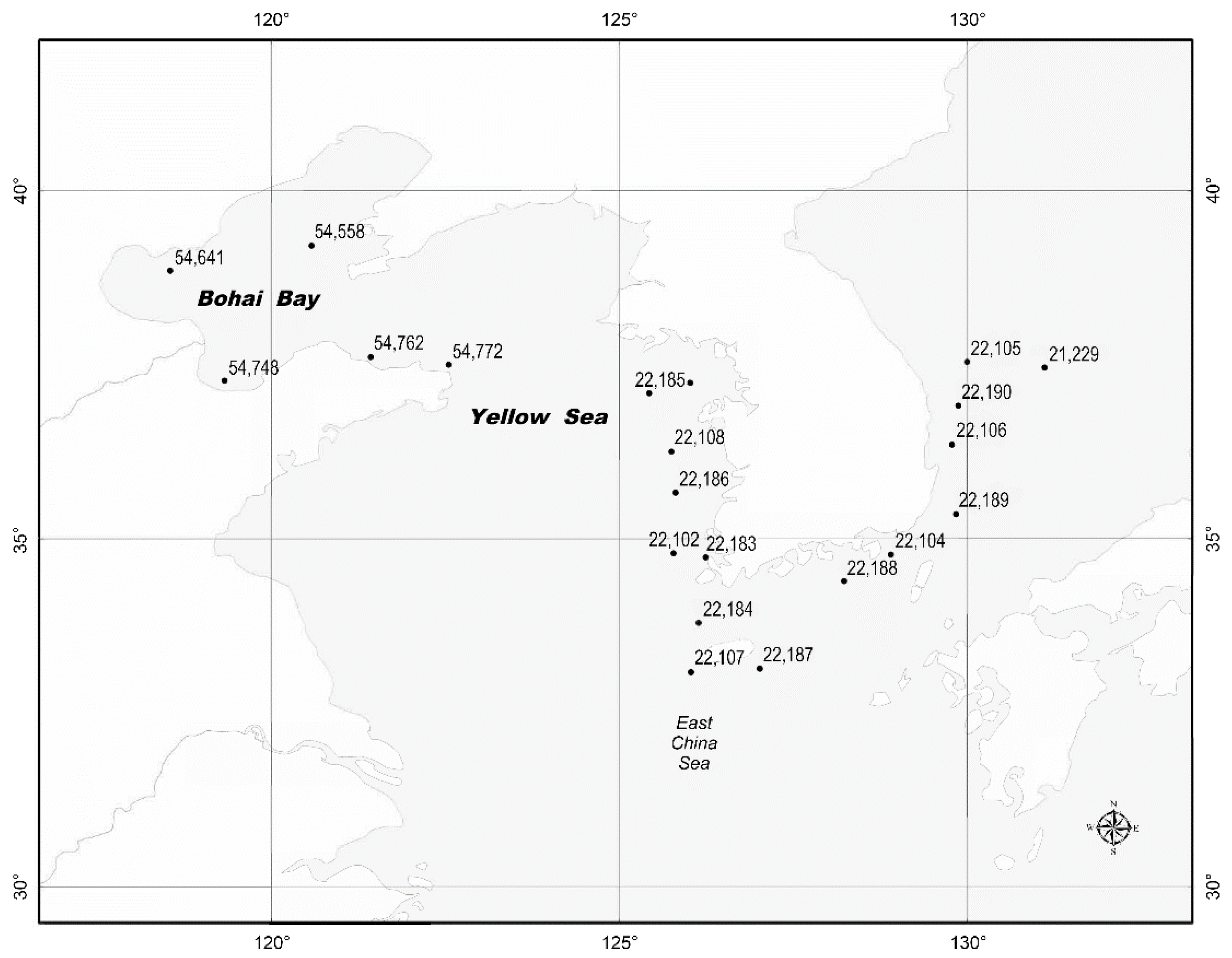
The verification scope of fusion SST products included the Bohai Sea, Yellow Sea, and offshore of Korea. The buoy SST data were obtained from the China Integrated Meteorological Information Service System (CIMISS) of the CMA, and 16 buoy sites around the vicinity of Korea and five buoys in Bohai Bay were selected for the quality assessment (Figure 1); all sites were located offshore. Owing to little buoys being distributed on the Bohai Sea and Yellow Sea, the verification is dependent on different factors; for example, the near coast area represents the key location for SST quality improvements because the coastline has a certain influence on the SSTs retrieved using microwave remote sensing and this can result in a decrease in SST accuracy. Moreover, the larger daily variation in SST causes the SST error to increase.
3.1.2. Verification Method for CODAS Fusion SSTs
For verification, we adopted the assessment method issued by CMA, i.e., the Actual Analysis Product Quality Assessment Specification (2019 version). In this method, the mean error (ME) and root-mean-square error (RMSE) are used to examine the accuracy of fusion SST products. The assessment equations are as follows:
Equation (4) provides the mean error and Equation (5) provides the root-mean-square error.
In the above equations, Oi is the observation value of the buoy site, Gi is the interpolated value of the CODAS fusion SST at the buoy site, and N is the monthly total sample number.
3.2. Quality Assessment of CODAS Fusion SSTs
3.2.1. Quality Assessment Procedure for CODAS Fusion SSTs
The assessment process for SSTs was as follows. First, the grid data of the fusion SST were interpolated to the buoy sites, in which the inverse distance interpolation method was adopted. Then, the accuracy of the fusion SSTs was inspected using the above verification method. Since the buoy SSTs were hourly SSTs and the CODAS fusion SSTs were daily or 6 h mean SSTs, hourly buoy SST data were processed into 24 h-averaged values for comparison with the daily CODAS SSTs and 6 h averaged values. Thus, it was possible to attain temporal correspondence between the two types of data.
3.2.2. Assessment Results for the Daily Fusion SSTs of CODAS
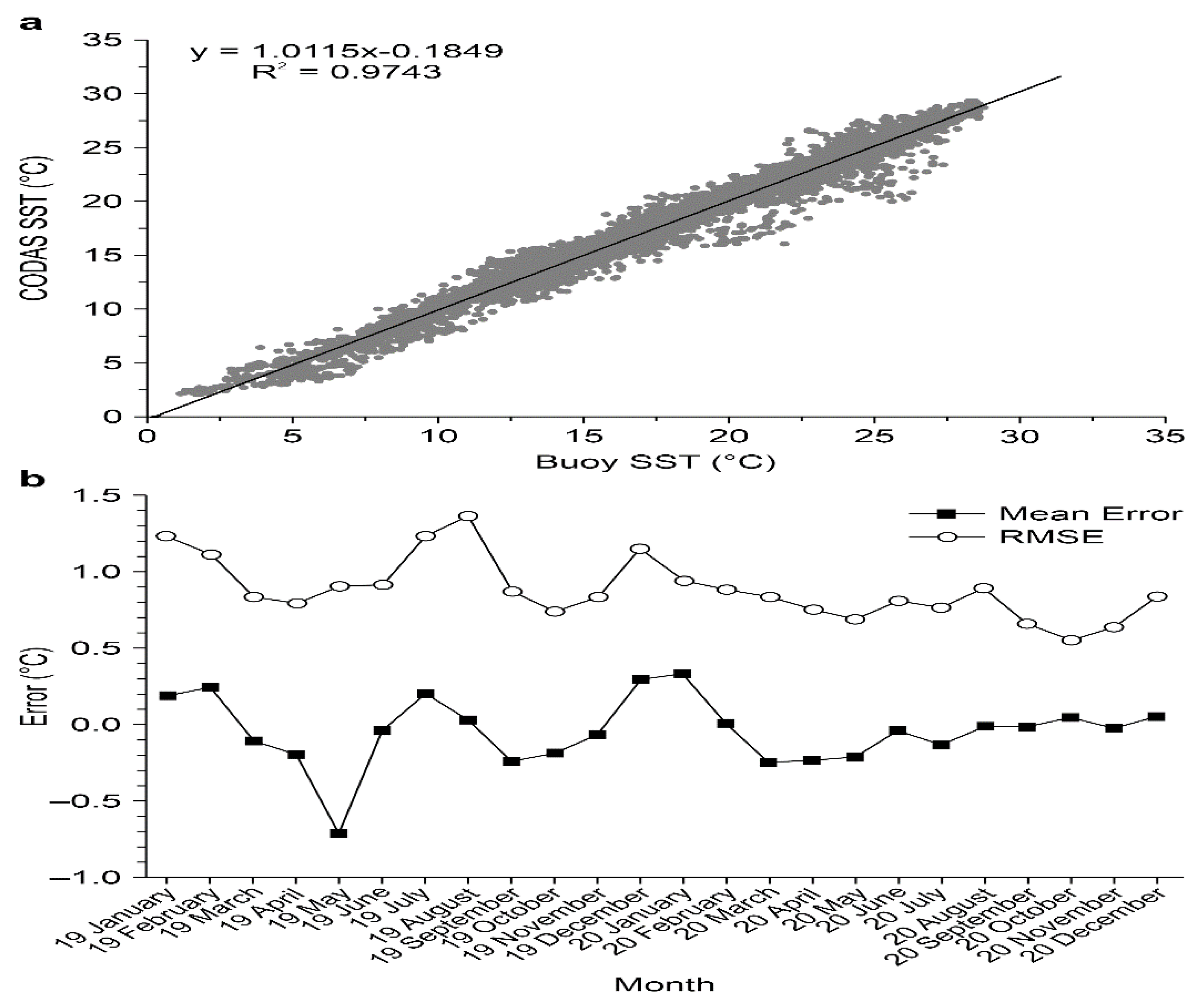
The scatter plots of daily fusion SST and buoy SST were drawn using 5512 sets of SSTs (Figure 2a). The two kinds of SSTs showed good fitting results. The fitting equation was y = 1.0115x + 0.1849, where x is the buoy SST and y is the CODAS fusion SST. The mean error and RMSE were −0.015 °C and 0.996 °C, respectively.
Tang et al. [15] researched the SST errors of different fusion methods and found that the mean errors of different fusion methods were between 0.15 °C and 0.18 °C, and that the RMSEs were between 0.72 °C and 0.83 °C. Sakaida et al. [27] pointed out that the biases and RMSEs of Global Imager (GLI) SSTs are 0.03 K and 0.66 K for daytime and −0.01 K and 0.70 K for nighttime. Cloud contamination is a key factor that influences the retrieval of SSTs, with the corresponding results being 3 °C colder than other observations [28], particularly in areas where marine stratiform clouds are seasonally prevalent and where the >1.0 K increase in RMSE values from June to August can be found in the daytime. Tang et al. revealed that the mean error of the CODAS fusion SST was more than 10 times smaller than the mean error obtained in their research [15]; this was similar to the results obtained by Sakaida et al. [27]. The RMSE was slightly larger than that found in these two previous studies.
Figure 2b shows the time series of the monthly mean errors and RMSE of the daily CODAS SST and the daily buoy SST of 21 buoy sites from January 2019 to December 2020. The variation in the monthly mean error ranged from −0.71 to 0.33 °C, and the monthly RMSE was 0.64–1.36 °C. Both the monthly mean deviation and RMSE of CODAS fusion SSTs showed a significant improvement from January 2019 to December 2020. However, there still were larger monthly RMSEs in summer and winter, which occurred because of the greater number of cloudy days in summer and the greater number of foggy days in winter in north China than in the other seasons. Clouds and fog may affect the accuracy of the retrieved SSTs from satellite remote sensing owing to the threshold variation of cloud masks in different places [29], and this could result in an increase in the mean error and RMSE.
3.2.3. Assessment Results for the 6 h Fusion SSTs of CODAS
Figure 3a shows the scatter plots of 6 h fusion SST and 6 h buoy SST with 16,753 sets of SST. The fitting equation was y = 0.9902x + 0.1423, where x is the buoy SST and y is the CODAS fusion SST. The fusion SST and buoy SST showed good fitting results.
Figure 3b shows the time series of monthly mean errors and RMSEs of the 6 h CODAS fusion SST and the 6 h buoy SST at 21 buoy sites from July 2019 to June 2020. Their monthly mean errors ranged from −0.26 to 0.45 °C, and the monthly RMSE was 0.64–1.73 °C. The mean error and RMSE of all samples for 13 months were 0.04 °C and 1.06 °C, respectively. The 6 h CODAS fusion SST had a similar error level as that of the daily fusion SST, and larger errors also occurred in summer and winter.
4. Influence of Different SSTs on the Simulation Results for Sea Fog
4.1. Characteristics of Fog Events around Bohai Bay
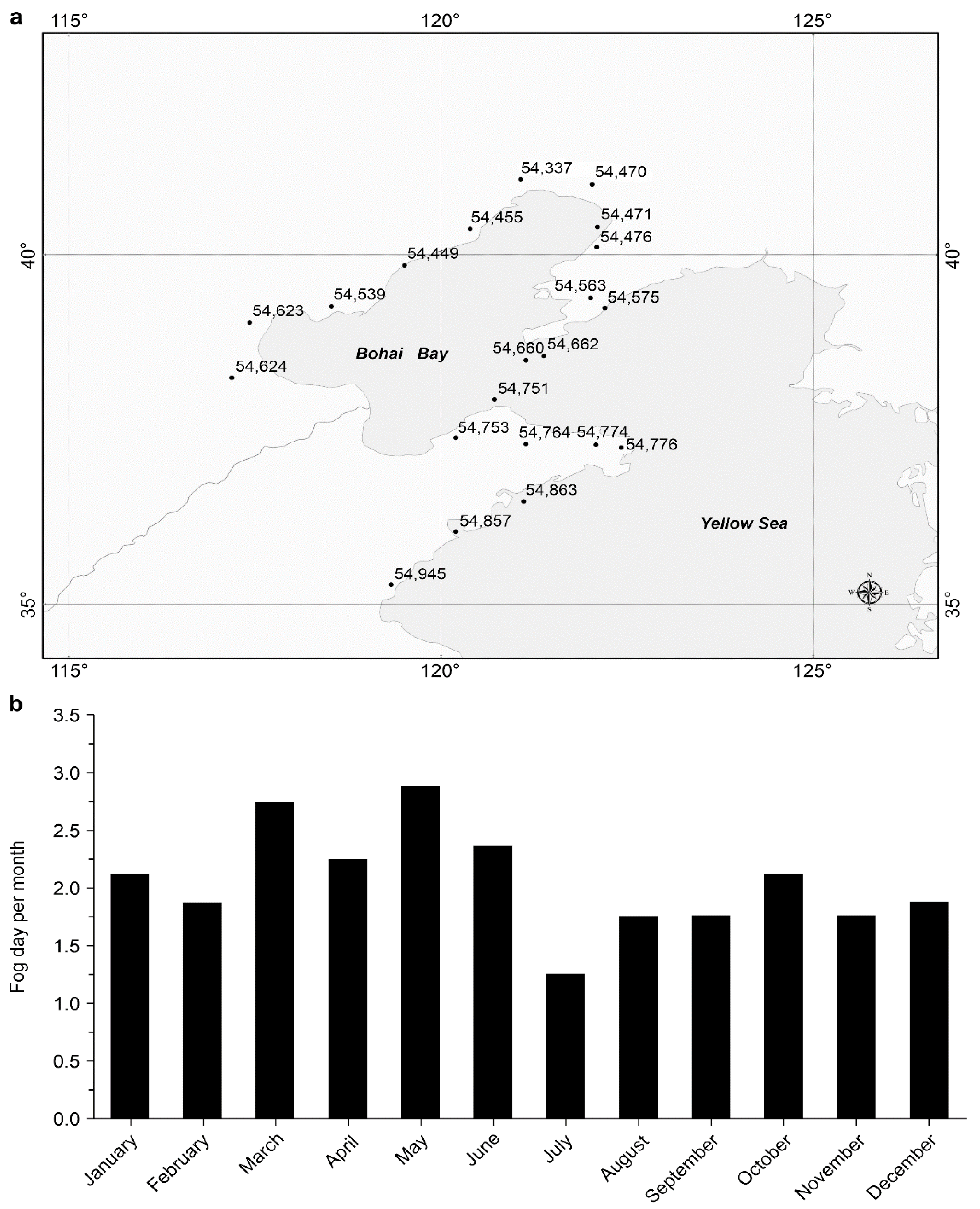
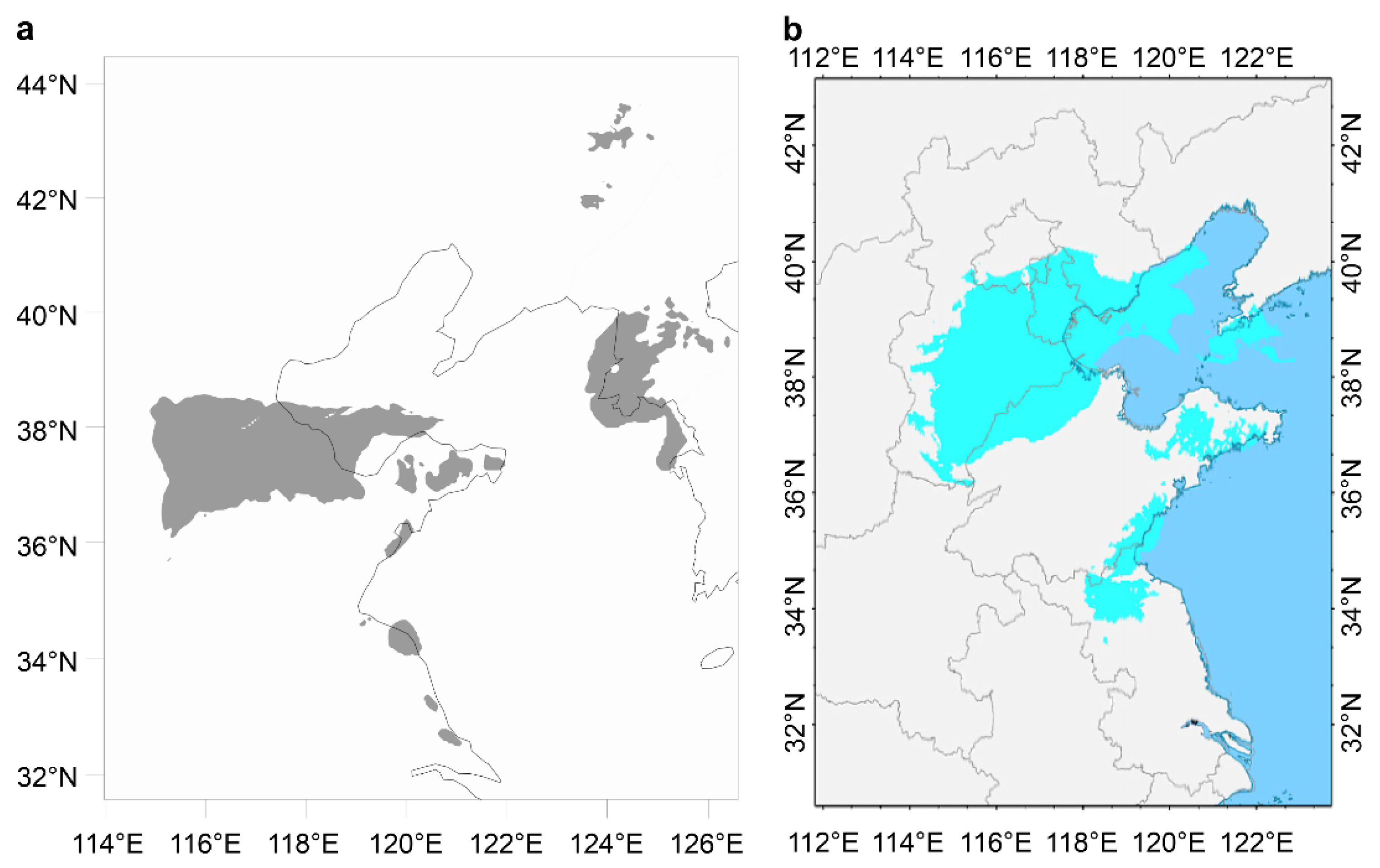
Errors in SST may affect the prediction accuracy of NWPs for fog, which is a key weather phenomenon that influences urban and oceanic traffic. To understand the characteristics of fog in Bohai Bay, the monthly characteristics of coastal fog events were analyzed in terms of 3-h surface meteorological data collected at 21 observation stations in Bohai Bay from 2011 to 2018 (Figure 4a).
Regional fog occurs every month around the Yellow–Bohai region (Figure 4b). Fog is most frequent in January in winter, while March and May are the most popular times for fog in spring. June has the highest number of foggy days in summer, while October has the maximum number for foggy days in autumn. Additionally, Zheng et al. pointed out that there is also a high frequency of fog events at station 54,455 in October [30]. The monthly characteristic chart shows that fog peaks in the region generally correspond to the period of the larger temperature difference between the air and sea.
4.2. Information on Fog Events and the Simulation Scheme
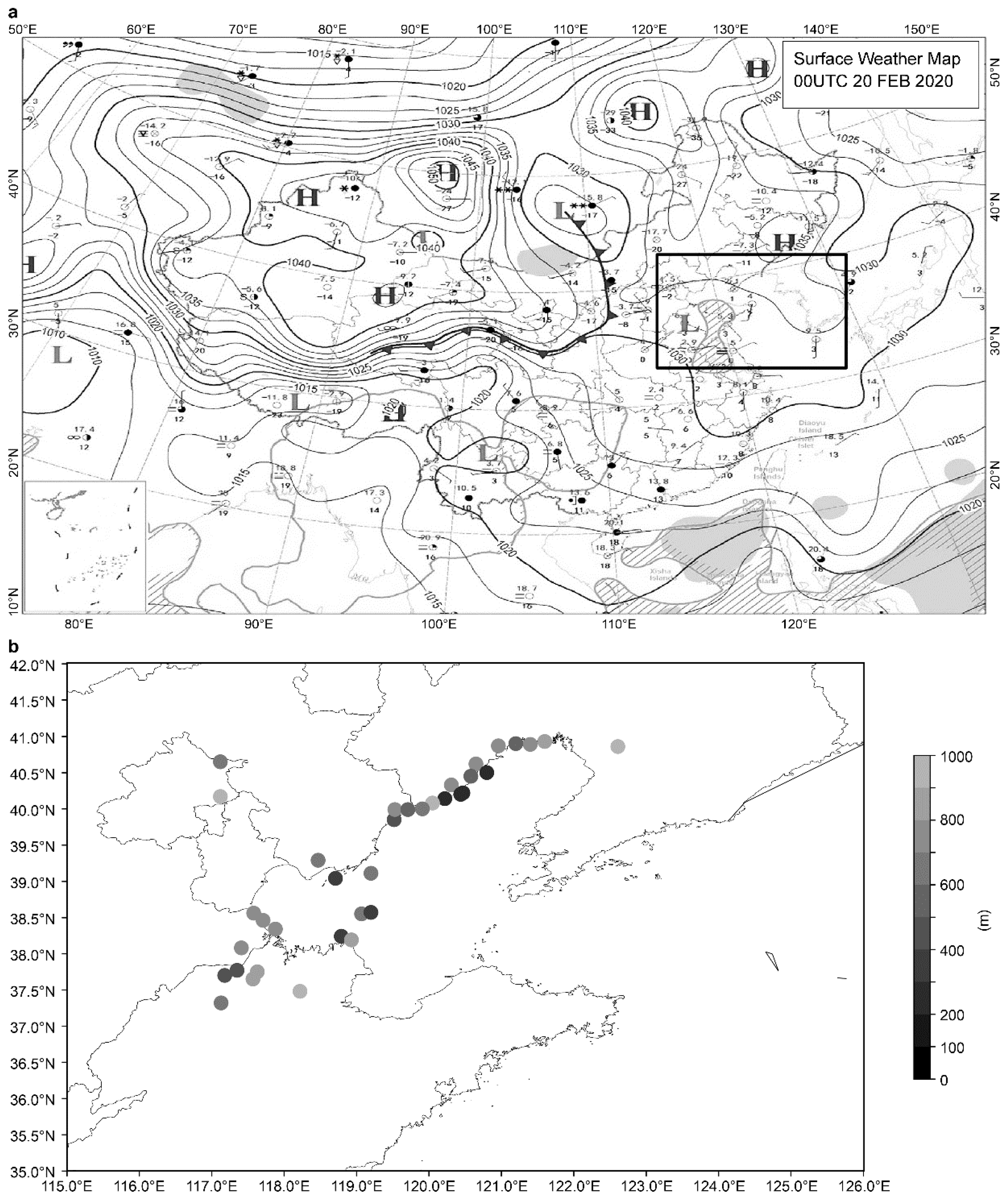
A notable fog event was selected for the simulations, which involved thick fog in Bohai Bay on 19–20 February 2020. The satellite image on the morning of February 19 showed the thick fog along the Bohai coast, and it extended westward over the Beijing–Tianjin–Hebei region at 00:00 (UTC) on February 20. Simultaneously, fog also appeared in the Bohai Strait and along the Shandong coast (Figure 5a). The surface weather map showed that the fog area was located at the back of a high-pressure system where the sparse isobars were conducive to the zone of fog formation (Figure 5b).
The temperature difference field between different SST products was used as to determine the impact of the SST error, which may have an influence on the temperature differences between the air and sea playing an important role in fog formation [31,32,33,34]. In the simulated fog zone, 0.05 g/kg of liquid water content (the sum of cloud water and cloud ice) in the lowest layer of the model was used as the threshold for fog identification.
The model parameters of the numerical simulations refer to the WRF model of the Tianjin Meteorological Administration. The horizontal resolution of the grid was 5 km, with 51 layers being in the vertical direction. The model center was located at 115° E, 40° N. The WRF single-moment (WSM) level 6 (graupel) method was selected as the microphysics scheme, and the Yonsei University (YSU) scheme was used for the boundary layer; the Noah scheme was used for the land surface, and the Rapid Radiative Transfer Model for General Circulation Model (RRTMG) scheme was used for both long-wave (wavelength more than 4.0 µm) and short-wave (wavelength less than 4.0 µm) radiations [35,36]. Owing to the occurrence of fog during stable weather conditions, the Kain–Fritsch cumulus parameterization scheme was chosen for performing the simulations.
The experimental scheme was divided into the following two groups: a control group and a contrast group. The surface temperature of FNL was used as the control group SST, and CODAS SST was used as the contrast group SST. The simulation scheme is shown in Table 1. The start time of simulation is at 00:00 UTC on 18 February 2020, the end time is at 12:00 UTC on 21 February 2020, the forecast horizon is 84 h.
4.3. Simulation Results of Daily CODAS SST
4.3.1. SST Field for Simulations
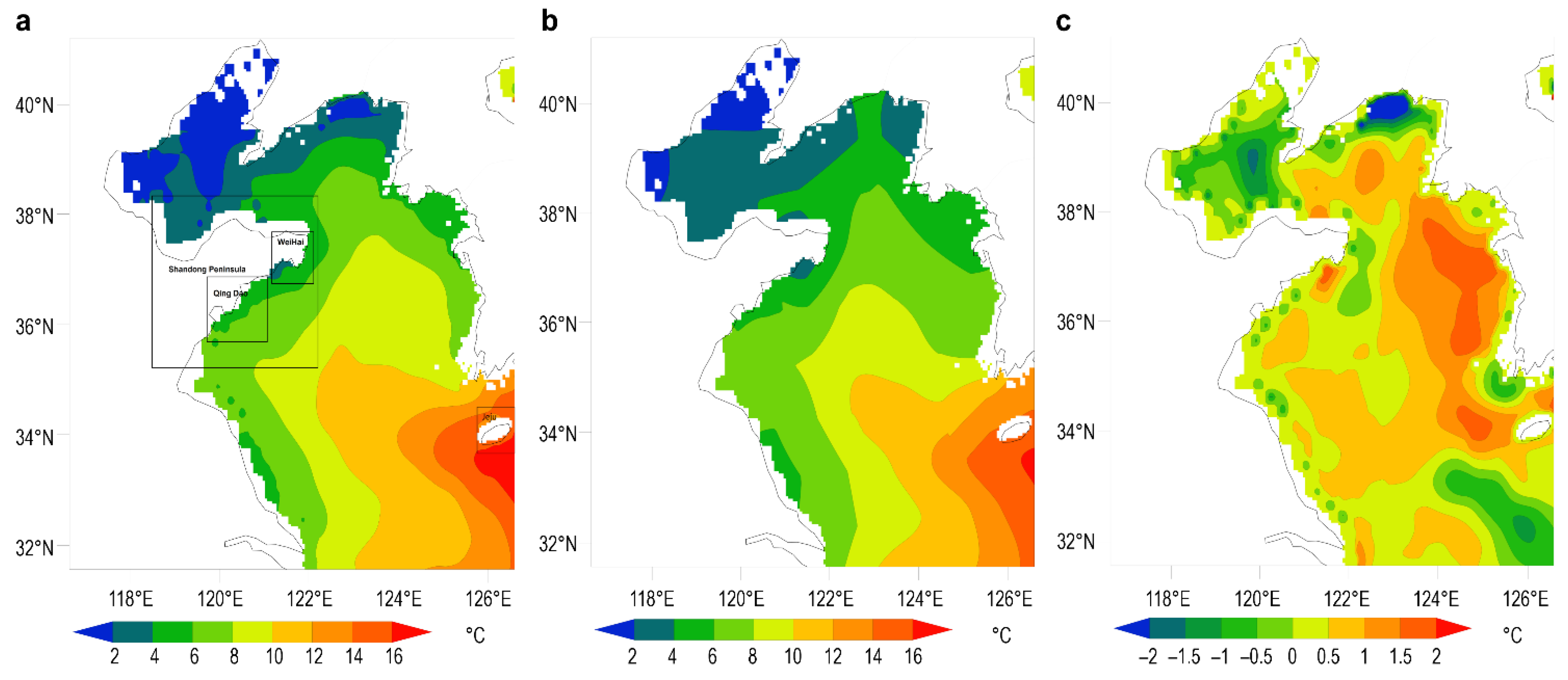
Figure 6a shows the CODAS SST as the control group, and Figure 6b shows the FNL SST as the contrast group. Figure 6c presents the temperature difference between the CODAS SST and FNL SST; the results show that the fusion SST had lower values in Bohai Bay and higher values in the eastern part of the Yellow Sea.
The fusion SST in most regions of Bohai Bay was approximately 0 to 1 °C lower than the FNL SST, and the fusion SST was lower than the FNL SST by 1 to 2 °C at the center of Bohai Bay. In most areas of the Yellow Sea, the fusion SST was 0–2 °C higher than that of the FNL. However, the fusion SST near WeiHai was approximately 0.5 °C lower than that of the FNL, and more than 2 °C lower than the FNL SST at the northern part of the Yellow Sea. Fusion SSTs can cause the distribution of the FNL SSTs to change in the lower boundary condition of the numerical model.
By comparing the simulated fog distribution with the FY4A monitoring fog (Figure 7), we can see that the simulated result is smaller than the satellite monitored fog area. However, the simulated fog region is included in the satellite monitoring fog area.
4.3.2. Influence of SST Differences on Sensible Heat Flux between the Air and Sea
At 00:00 (UTC) on 20 February, the SST of the CODAS contrast group showed that the sensible heat flux of air and sea and its flux difference were positive in most areas of the Yellow–Bohai Sea. However, negative sensible heat flux also appeared in certain regions (Figure 8). Moreover, the difference chart of sensible heat flux showed that the variation in sensible heat flux was positively correlated with the SST changes (Figure 8b). For example, the variation in sensible heat flux was more sensitive to SST changes in the northern and southern parts of the Yellow Sea and in the sea around the Shandong Peninsula, especially the waters near Jeju Island; its variation ratio exceeded 5 W/(m2·°C). The SST change can impact atmospheric heat variation through the sensible heat flux variation.
4.3.3. Influence of SST Differences on Temperature in the Fog Region
Air temperature is a key atmospheric heat factor that has a close relationship with the sensible heat flux, which led to a significant positive correlation between the air temperature and SST difference. Moreover, the extent of the larger air temperature variation between the CODAS simulation and FNL simulation was related to the value and area of the SST anomalies (Figure 9). Air temperature was more sensitive to the SST change in the center of Bohai Bay and the southern part of the sea area near the Shandong Peninsula and the coastal zone. The ratio of air temperature variation and SST change exceeded 1. However, the change was not linear; it was also affected by weather processes. In general, the SST change can have an influence on the air temperature of fog areas.
4.3.4. Influence of SST Differences on Specific Humidity and Liquid Water in the Fog Region
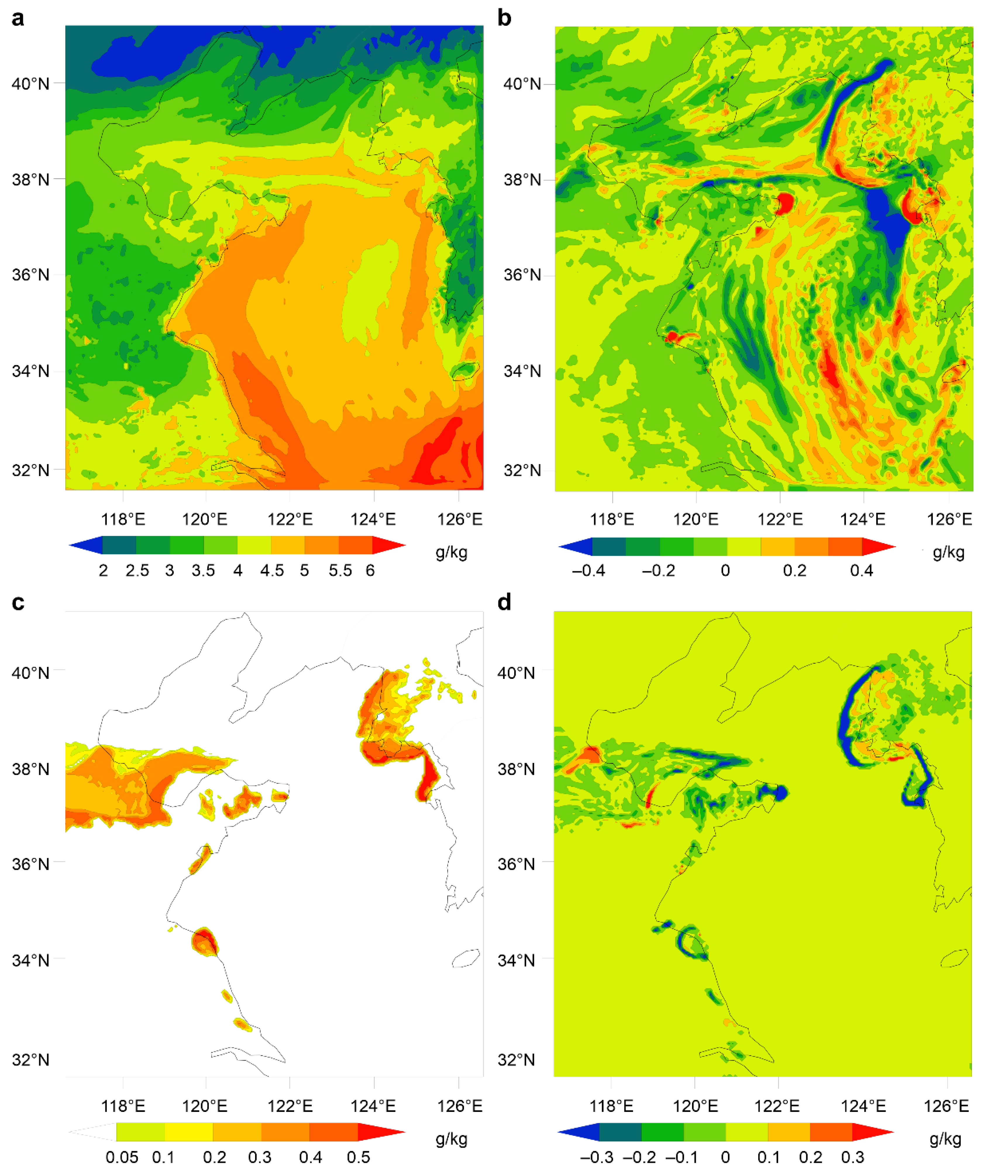
Figure 10 shows the distribution of the simulated liquid water content and specific humidity, and the differences in liquid water content and specific humidity between the CODAS simulation and the FNL simulation. There was a complex relationship between the specific humidity variation and SST change. A positive correlation appeared in Bohai Bay, but positive or negative changes appeared alternately in the Yellow Sea (Figure 10b). The negative variation of specific humidity weakened the former high specific humidity in this area, and the change ratio of specific humidity and SST change reached as high as 0.4 g/(kg·°C).
Liquid water content is the key parameter for determining fog visibility in the NWP model. Figure 10c shows that there were larger foggy areas in Bohai Bay and its coastal regions of the Shandong Peninsula and Sulu, as well as the northeastern part of the Yellow Sea. Meanwhile, the liquid water content increased in the western part of the foggy area in Bohai Bay, while it clearly decreased in the foggy area of Shandong Peninsula, coast of Sulu, and the northeastern part of the Yellow Sea (Figure 10d).
According to the SST variation (Figure 6c), lower SSTs in Bohai Bay cause the liquid water content to increase in the nearby sea fog, which fits the mechanisms of advection fog formation by warm air flowing over colder water because of more condensate being produced when the temperature contrast between the upstream warmer and colder surface is larger. Meanwhile, higher SSTs in the central and northern Yellow Sea cause the liquid water content to decrease in the sea fog region. The warm SSTs may increase the temperature of the air above the sea surface, which can evaporate the liquid water in the fog region.
In general, the daily CODAS SST significantly changed the simulated liquid water content of WRF in the simulated fog area of the Bohai Bay, as compared to the daily FNL SST.
4.4. Simulation Result of CODAS 6 h SST
CODAS 6 h SST shows the spatial variation in more detail compared to those of the CODAS daily SST and FNL SST, as shown in Figure 11a; therefore, it was necessary to analyze if the difference had an influence on the sea fog simulation. Three fog simulation schemes were designed using different SSTs: the 6 h scheme with CODAS 6H SST being the lower boundary condition of WRF, daily scheme with CODAS daily SST, and FNL scheme with FNL 6 h SST.
4.4.1. Comparison of Sea Fog Simulation with the Three SST Schemes
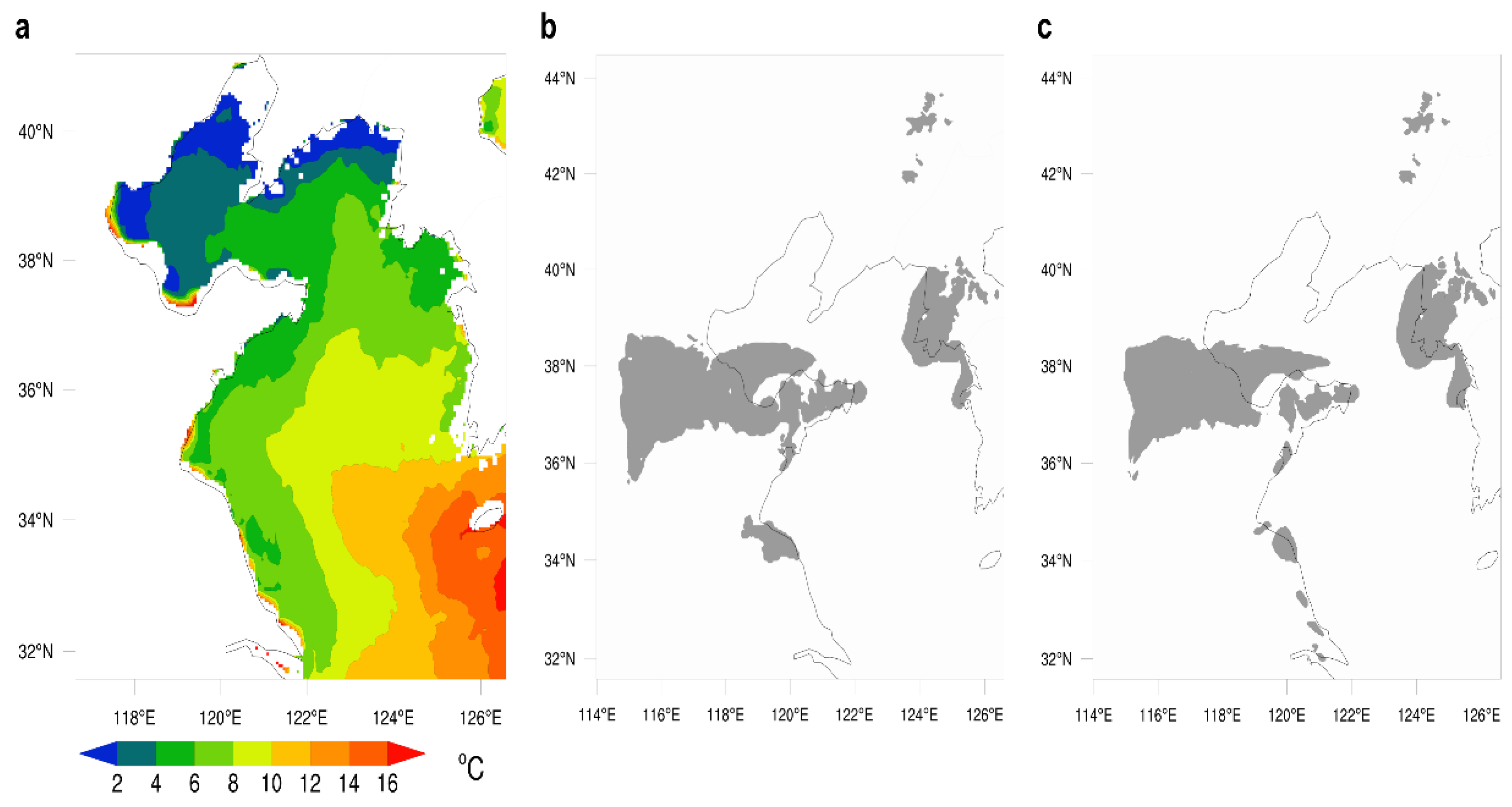
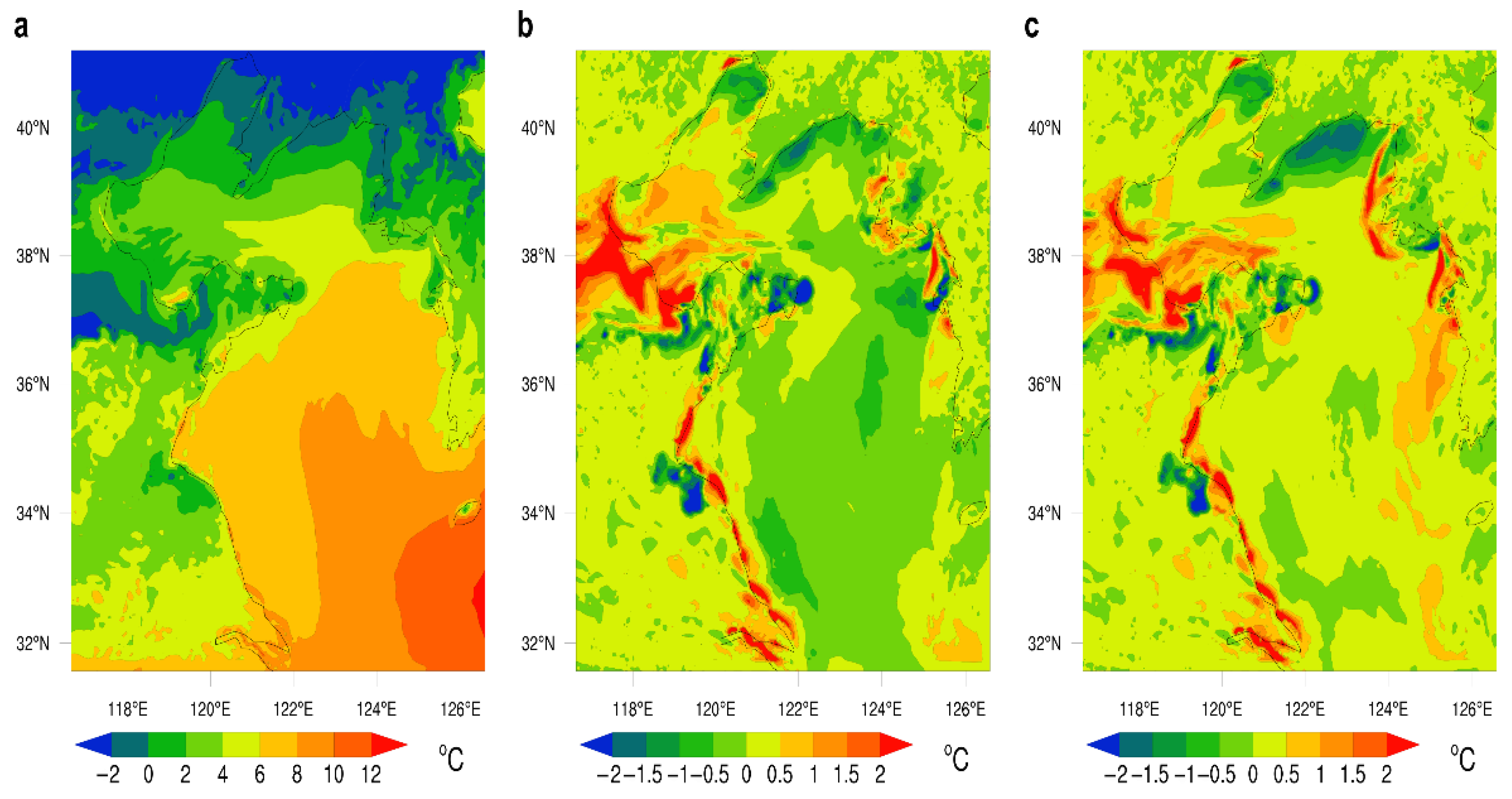
At 00:00 on 20 February 2020, the CODAS 6 h SSTs exhibit obvious regional differences between the northern and the southern regions of the Yellow Sea and Bohai Sea (Figure 11a). The lowest SST can reach 0 °C in the north of the simulated area, and the highest SST is more than 15 °C in the southeast.
For most areas, the simulated fog area using the 6 h scheme is similar to that simulated using the other two schemes; however, it is larger than that of the other schemes in the vicinity of Shandong Peninsula, which may be due to the spatial detail difference of CODAS 6 h SST (Figure 7a and Figure 11b,c).
4.4.2. Spatial Differences of the Three SST Schemes
To understand the effect of high temporal and spatial resolution SST on NWP fog simulation, the differences are analyzed by comparing the simulations of the three SST schemes.
The difference between the results obtained by the 6 h scheme and daily scheme shows there are more detailed spatial variations in the simulated area. In the Bohai Sea, the SST of the 6 h scheme is 1–2 °C higher than that of the daily scheme. However, it is lower by 0.5 °C than the SST of the daily scheme in most areas of the Yellow Sea, and even lower by 1–2 C in the central and eastern areas of the Yellow Sea (Figure 12a).
The difference between the results of the 6 h scheme and FNL scheme is significant, and ranges from −2 °C to +2 °C (Figure 2b). The SST of the 6 h scheme is 1–2 °C higher than that of the FNL scheme in the middle eastern part of the Bohai Sea and the northern and eastern parts of the Yellow Sea. However, the SST of the 6 h scheme is lower than that of the FNL scheme in the middle eastern part of the Yellow Sea, while being lower by 2 °C in the coastal area at the north of the Yellow Sea.
Compared with the fog area observed by satellite, the fog area simulated using the FNL scheme is smaller than that in the west of the Bohai Sea and Shandong Peninsula; however, it is larger than that observed in the northeastern parts of the Yellow Sea. The fog area simulated using the daily scheme is similar to that simulated by the FNL scheme; the coverage and intensity of both the simulated fog areas are relatively large. The fog area simulated using the daily scheme is similar to the fog distribution in the northeastern part of the Yellow Sea. Compared with the above-mentioned schemes, the fog coverage simulated using the 6 h scheme is enlarged in the west of the Bohai Sea and Shandong Peninsula. However, the simulated fog area decreases in the northeastern parts of the Yellow Sea, which is in accordance with the actual fog area. The 6 h scheme has a different impact on fog simulation in different simulation areas.
4.4.3. Effect of Different SSTs on Sensible Heat Flux at Air–Sea Interface
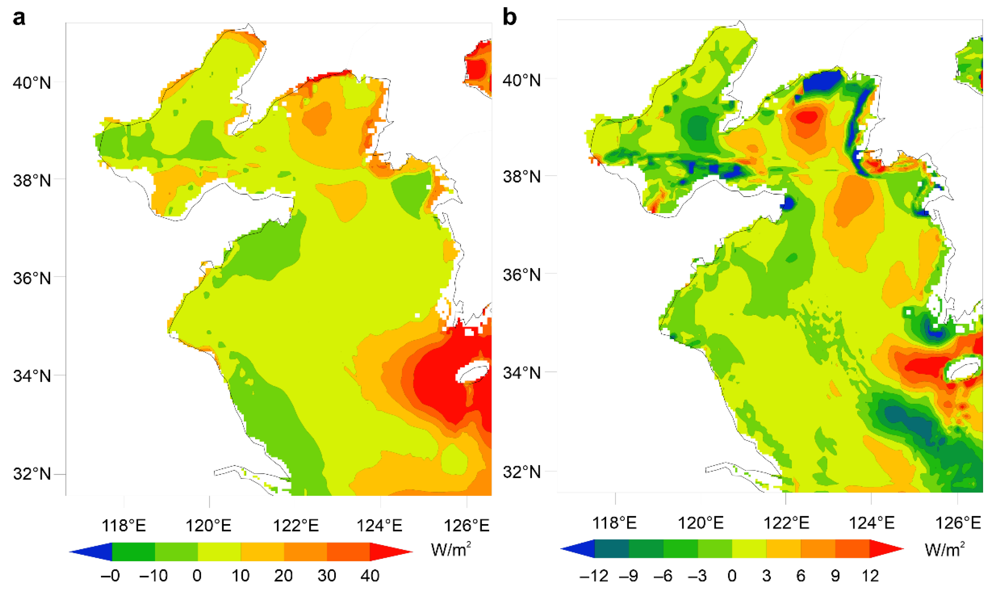
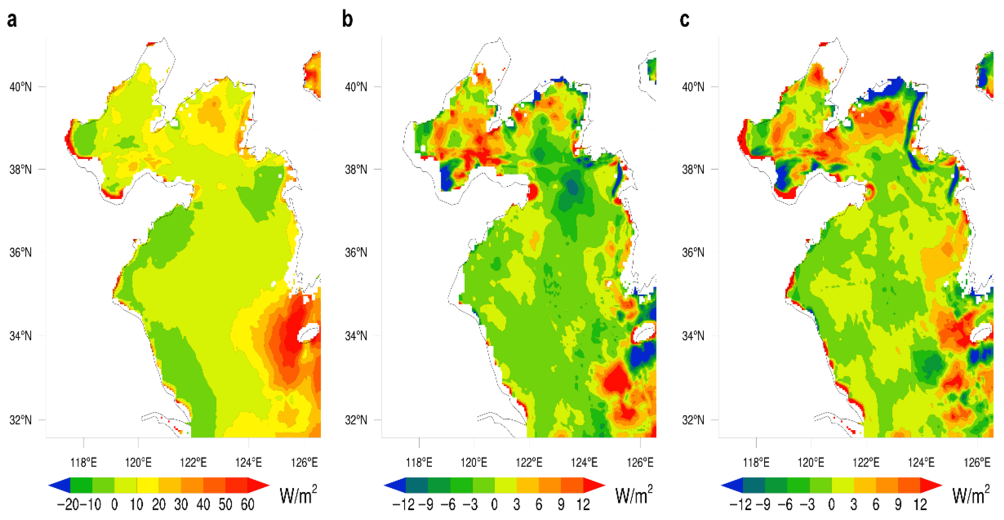
As shown in Figure 13a, the sensible heat flux simulated using the 6 h scheme is generally positive in most areas of the Yellow Sea and Bohai Sea; it exhibits a value of approximately 10–20 W/m2, which exceeds 30 W/m2 in the northern Yellow Sea. The high sensible heat flux exists in the southeast region of the simulated area; it exhibits values exceeding 50 W/m2. These phenomena imply that the atmosphere absorbs heat from the ocean in most areas of the Bohai Sea and Yellow Sea. However, the sensible heat flux is negative in the western part of the Bohai Sea, as well as in parts of the east coast and northeastern parts of the Yellow Sea; i.e., the negative sensible heat flux is within −10 W/m2.
The sensible heat flux simulated using the 6 h scheme and daily scheme shows that a negative difference occurs at the middle of the Yellow Sea, where the absolute difference exceeds 6 W/m2 (Figure 13b). This shows that the sensible heat flux of the 6 h scheme is smaller than that of the daily scheme. A positive difference in the sensible heat flux occurs in most areas of the Bohai Sea, with the difference being more than 12 W/m2 in the eastern Bohai Sea.
The differences between the simulations of the 6 h scheme and FNL scheme show some variation comparable to those between the simulations of the 6 h scheme and daily scheme. In Figure 13c, the significantly positive and negative variations in the central Bohai Sea can be observed. The negative value is less than −12 W/m2 and the positive value is greater than −12 W/m2 in the Bohai Sea. However, the area covered by the negative values is larger than that observed when comparing the 6 h scheme and daily scheme in the Bohai Sea, while it is smaller for the same comparison at the middle of the Yellow Sea.
In general, the variation in the sensible heat flux exhibits increase or decrease to the positive or negative differences changing among the three SST schemes with regard to spatial distributions, and the average ratio of the sensible heat flux difference to the SST difference can reach 6 W/m2.
4.4.4. Difference in Temperatures Simulated Using Three Schemes in Foggy Area
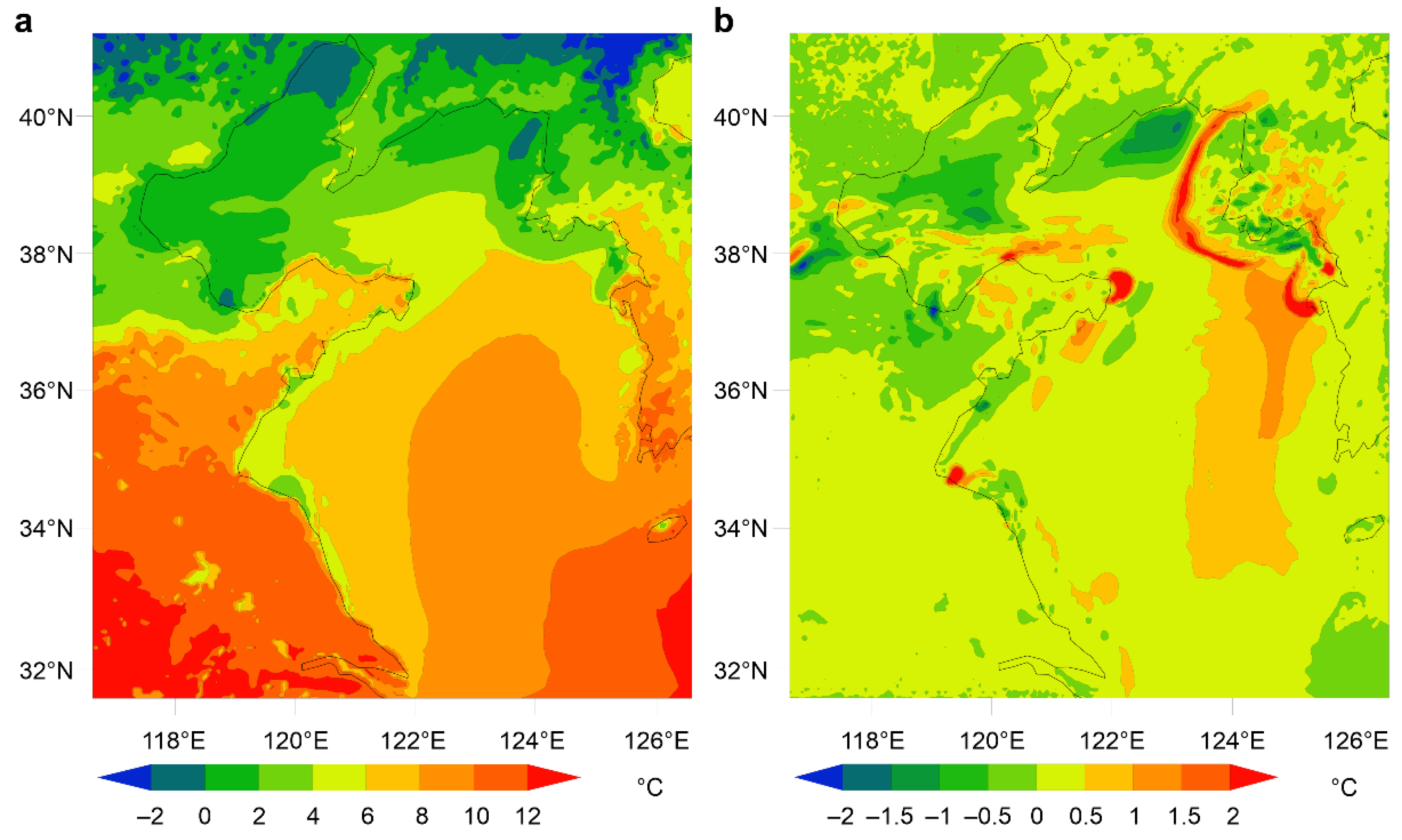
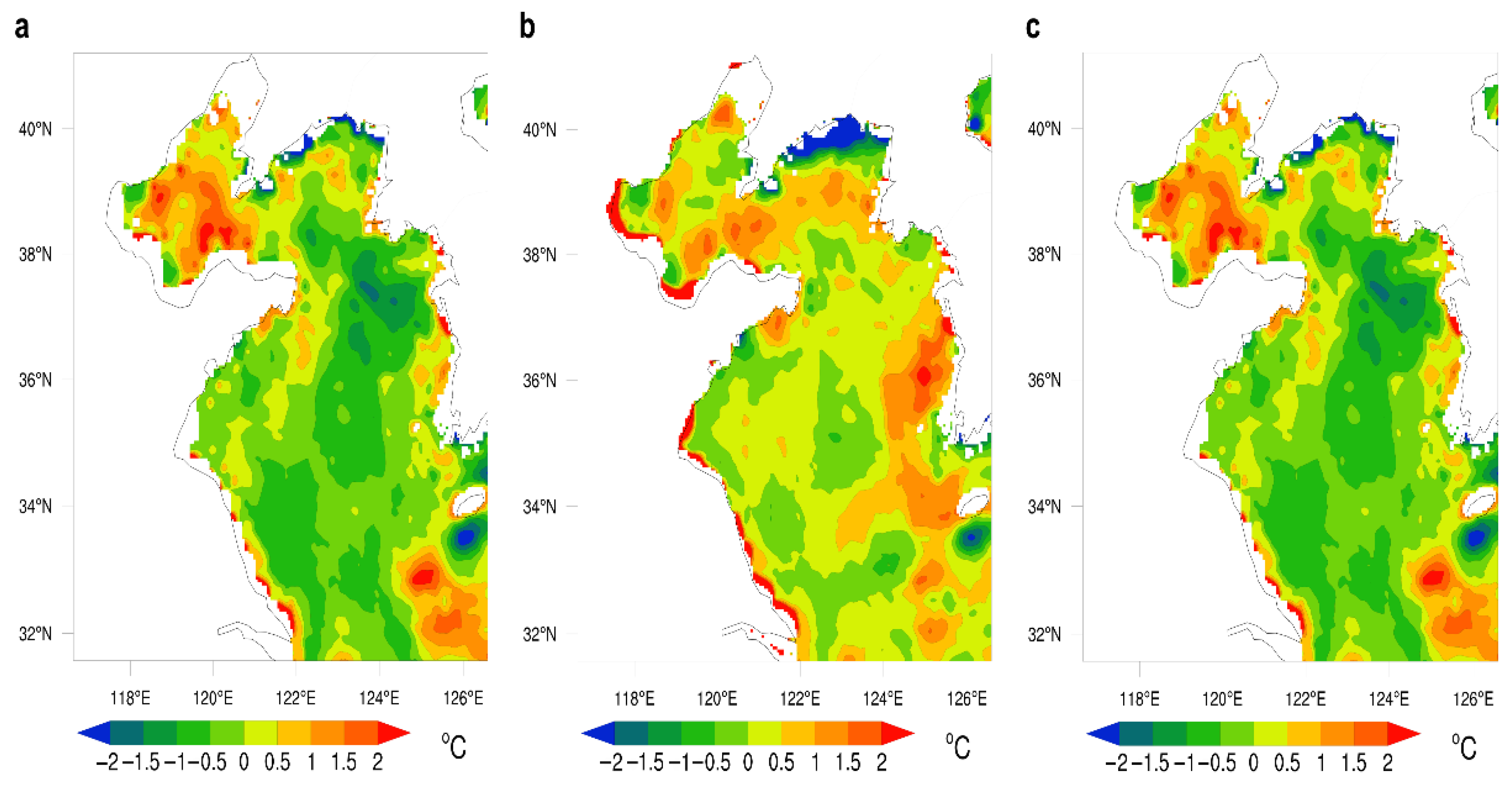
The result of the 2-m air temperature with the 6 h scheme shows there is obvious gradient difference from north to south in the simulation area, which is similar to the SST distribution (Figure 14a). Meanwhile, SST is slightly higher than that obtained with the 2-m air temperature, with the temperature difference between the SST and air temperature being positive. The distribution of the positive sensible heat flux coincides with the area of the positive temperature difference between SST and air temperature.
The 2-m temperature between the 6 h scheme and daily scheme can reach 1–2 °C (Figure 14b), and the difference in the distribution is similar to that observed with SST distribution. An SST difference of more than 1 °C is consistent with a 2-m temperature above 0.5 °C in the middle of the Bohai Sea, and the SST difference lower than 1–2 °C is consistent with a 2-m temperature lower than 0.5 °C in the north coast and middle of the Yellow Sea.
The temperature difference between the 6 h scheme and FNL scheme shows that the temperature difference is higher than 1–2 °C in the southern Bohai Sea and the eastern Yellow Sea, and lower than −2 °C along the northern coast of the Yellow Sea. The spatial distribution of the air temperature difference is basically consistent with the SST difference of the 6 h scheme and FNL scheme, and the value of the air temperature difference is lower than the SST difference. The air temperature difference is proportional to the SST difference (Figure 14c).
4.4.5. Difference in Specific Humidity and Liquid Water Content between the Three SST Schemes
The spatial distribution of the 2-m specific humidity with the 6 h scheme presents significant nonuniformity in the fog region. Moreover, the specific humidity over ocean is higher than that over land (Figure 15a).
The difference in the 2-m specific humidity is ±0.2 g/kg when comparing the 6 h scheme and daily scheme in most areas of the Yellow Sea and Bohai Sea, while a positive difference of more than 0.3–0.4 g/kg is also observed (Figure 15b). However, the 2-m specific humidity varies differently with SST in different simulation areas. For example, the simulation results of 6 h scheme show that the lower SST corresponds to the lower specific humidity in the northern Yellow Sea, while the higher SST also corresponds to a lower specific humidity in the central and eastern Yellow Sea. This phenomenon may indicate that the specific humidity not only depends on the variation of SST, but also is impacted by the meteorological conditions.
At the same time, the difference in the 2-m specific humidity simulated by the 6 h scheme and FNL scheme also shows the same characteristics (Figure 15c), which implies that SST could have an influence on the 2-m specific humidity; however, it does not have a significant proportional relationship with the 2-m specific humidity.
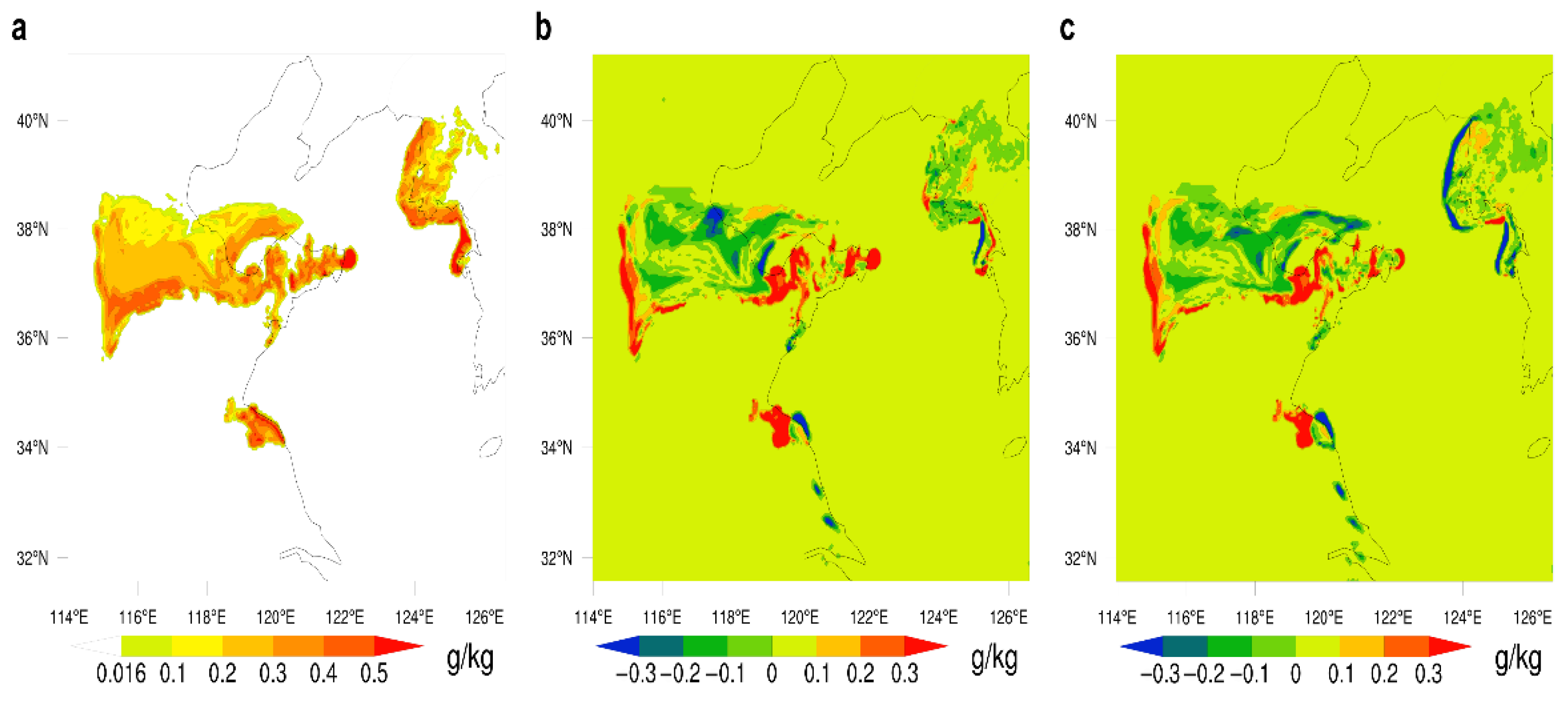
The distribution of the liquid water content simulated using the 6 h scheme shows that there are three fog areas. The liquid water content in the north side of the fog area over the Bohai Sea is less than that in the south side where the liquid water content is more than 0.4 g/kg in the Shandong Peninsula. In the fog area of the northeastern Yellow Sea, the liquid water content in the west is higher than that in the east (Figure 16a).
The analysis of liquid water content with the three SST schemes shows that the SSTs have an influence on the liquid water content. A difference in liquid water content of more than 0.1 g/kg shows that liquid water content is sensitive to SST changes. In most fog areas, the higher SST corresponds to a lower liquid water content while the lower SST corresponds to a higher liquid water content (Figure 16b,c). This result is consistent with the discussion on the advection fog formation mechanism in the previous analysis of the CODAS daily SST simulation.
4.5. Summary of CODAS SST Simulation
To quantitatively analyze the overall relationship between the meteorological elements and SST changes, a sensitivity index is introduced to reflect the sensitivity of meteorological elements to sea surface temperature changes, which is the ratio of the absolute differences sum of meteorological elements to the sum of the absolute differences of SST in the Yellow Sea and Bohai Sea. The sensitivity index shows that the sensible heat flux on sea surface, air temperature, specific humidity, and liquid water content varies significantly with a change in the SST (Table 2). The sensible heat flux and 2-m air temperature exhibit a significant positive correlation with SST, with the average ratio of 0.528 °C/°C and 6.092 W/(M2·°C). Meanwhile, the liquid water content has a significant negative correlation with SST, with the ratio of −0.0143 g/(kg·°C). The specific humidity at 2 m is also affected by SST to a certain extent, with a ratio of 0.185 g/(kg·°C); however, the specific humidity is not directly proportional to SST variation.
The simulation results show that meteorology elements of sea fog in the Yellow Sea and Bohai Sea are sensitive to variations in SST. Higher SSTs can increase the air temperature above the sea surface, thereby allowing the sensible heat flux of the sea surface to strengthen and the atmosphere to be heated.
At the same time, warm SSTs correspond to a decrease in the liquid water content and lead to the simulated fog areas narrowing, which fits the mechanism of the advection cooling fog over the Yellow Sea and Bohai Sea; this is because sea fog is mostly suitable for air–sea temperature differences from −2 °C to 0 °C. However, the rising SST decreases the absolute value of the negative temperature difference between air and sea, or exhibits positive values that strengthen the turbulence activity of the air–sea interface and decrease the conversion from water vapor to liquid water. There is a non-linear interaction between SST and liquid water content, which can explain why warm SST is unfavorable for the formation and development of sea fog. However, the movement of warm air to the cold sea surface is conducive to the condensation of water vapor in the fog area promoting the development of sea fog.
5. Conclusions
The verification results show that the RMSE of the daily SST ranges from 0.64 to 1.36 °C (overall RMSE of 0.996 °C), and the RMSE of the 6 h SST varies from 0.64 to 1.73 °C (overall RMSE of 1.06 °C). The error levels between the fusion SST and observed SST are in a similar range to those published in the literature [15,27]. Moreover, the following conclusions were drawn from the numerical simulation results:
- (1)
- The simulation results show that the three SST schemes can greatly affect the sensible heat flux in the Yellow Sea and Bohai Sea. CODAS 6 h SST can provide a more detailed view of the variation in the sensible heat flux. All three SST schemes are significantly and positively correlated with the 2-m air temperature.
- (2)
- The CODAS 6 h SST scheme is better than the FNL SST scheme as regards the value and location distribution of the liquid water content in the modeled lower layer of the fog area. In particular, the lower 6 h SST more than other schemes is favorable for increasing the liquid water content, which fits the mechanisms of advection fog formation of warm air flowing over colder water.
- (3)
- The high spatial and temporal resolution SST in the Yellow Sea and Bohai Sea can significantly impact the fog forecast near the sea.
We believe that the fusion SST is an effective method to obtain SST data in remote ocean areas with scarce observation sites. The application of the first generation of actual fusion SST in China has been found to be conducive to improving the prediction accuracy of the NWP model for oceanic meteorology, and it can provide oceanic meteorology researchers with fine surface meteorological information for Bohai Bay. This development is favorable for meteorologists who study oceanic meteorology and will improve the accuracy of oceanic meteorological forecasts.
Author Contributions
Formal analysis, P.Q. and Z.L.; writing—original draft preparation, W.W.; visualization, X.G.; supervision, C.S.; methodology, B.X. All authors have read and agreed to the published version of the manuscript.
Funding
This research was funded by the Collaborative Innovation of Meteorological Science and Technique in Huang-Bohai Region program, grant number QYXM201801; and the key operational special plan of the China Meteorological Administration (YBGJXM (2020) 1A-10 and YBGJXM (2019) 01-09).
Data Availability Statement
All data were derived from the CMA operational network. The datasets used during the current study are available from the corresponding author on reasonable request.
Acknowledgments
We would like to thank Zhi-Hong Liao for providing the CODAS information and the CODAS 6 h SST.
Conflicts of Interest
The authors declare no conflict of interest. The funders had no role in the design of the study; in the collection, analyses, or interpretation of data; in the writing of the manuscript; or in the decision to publish the results.
References
- Khan, M.Z.K.; Sharma, A.; Mehrotra, R. Global seasonal precipitation forecasts using improved sea surface temperature predictions. J. Geophys. Res. Atmos. 2017, 122, 4773–4785. [Google Scholar] [CrossRef]
- Booth, J.F.; Thompson, L.A.; Patoux, J.; Kelly, K.A. Sensitivity of midlatitude storm intensification to perturbations in the sea surface temperature near the Gulf Stream. Mon. Weather Rev. 2012, 140, 1241–1256. [Google Scholar] [CrossRef]
- Cione, J.J.; Uhlhorn, E.W. Sea surface temperature variability in hurricanes: Implications with respect to intensity change. Mon. Weather Rev. 2003, 131, 1783–1796. [Google Scholar] [CrossRef] [Green Version]
- Tuleya, R.E.; Kurihara, Y.A. Note on the sea surface temperature sensitivity of a numerical model of tropical storm genesis. Mon. Weather Rev. 1982, 110, 2063–2069. [Google Scholar] [CrossRef] [Green Version]
- Wang, J.H.; Shao, C.X.; Miao, C.S.; Zhong, Q.; Wu, Y.R. Near-shore SST’s impact on typhoon return to the sea in numerical simulation. J. Trop. Oceanogr. 2012, 31, 106–115. [Google Scholar]
- Kim, C.K.; Yum, S.S. A numerical study of sea-fog formation over cold sea surface. Bound. Layer Meteorol. 2012, 143, 481–505. [Google Scholar] [CrossRef]
- Lenderink, G.; Meijgaard, E.V.; Selten, F. Intense coastal rainfall in the Netherlands in response to high sea surface temperatures: Analysis of the event of August 2006 from the perspective of a changing climate. Clim. Dyn. 2009, 32, 19–33. [Google Scholar] [CrossRef]
- Lombardo, K.; Sinsky, E.; Edson, J.; Whitney, M.M.; Jia, Y. Sensitivity of offshore surface fluxes and sea breezes to the spatial distribution of sea surface temperature. Bound. Layer Meteorol. 2018, 166, 475–502. [Google Scholar] [CrossRef]
- Wang, W.; Wu, D.Z.; Qu, P.; Li, Y.; Liu, L.L.; Wu, B.G. The retrieve and data fusion of the sea surface temperature with FengYun geostationary satellite data. J. Water Res. Ocean Sci. 2016, 5, 53–63. [Google Scholar]
- Khaleghi, B.; Khamis, A.; Karray, F.O.; Karray, F.O.; Razavi, S.N. Multisensor data fusion: A review of the state-of-the-art. Inform. Fusion 2013, 14, 28–44. [Google Scholar]
- Hilker, T.; Wulder, M.A.; Coops, N.C.; Linke, J.; McDermid, G.; Masek, J.G.; Gao, F.; White, J.C. A new data fusion model for high spatial-and temporal-resolution mapping of forest disturbance based on Landsat and MODIS. Remote Sens. Environ. 2009, 113, 1613–1627. [Google Scholar] [CrossRef]
- Zhang, W.; Li, A.N.; Jin, H.A.; Bian, J.; Zhang, Z.; Lei, G.; Qin, Z.; Huang, C. An enhanced spatial and temporal data fusion model for fusing Landsat and Modis surface reflectance to generate high temporal Landsat-like Data. Remote Sens. 2013, 5, 5346–5368. [Google Scholar] [CrossRef] [Green Version]
- Reynolds, R.W. A real-time global sea surface temperature analysis. J. Clim. 1988, 1, 75–86. [Google Scholar] [CrossRef] [Green Version]
- Reynolds, R.W.; Smith, T.M.; Liu, C.Y.; Chelton, D.B.; Casey, K.S.; Schlax, M.G. Daily high-resolution-blended analyses for sea surface temperature. J. Clim. 2007, 20, 5473–5496. [Google Scholar]
- Tang, S.L.; Yang, X.F.; Dong, D.; Li, Z. Merging daily sea surface temperature data from multiple satellite using a Bayesian maximum entropy method. Front. Earth Sci. 2015, 9, 722–731. [Google Scholar]
- Hosoda, K.; Kawamura, H.; Sakaida, F. Improvement of New Generation Sea Surface Temperature for Open ocean (NGSST-O): A new sub-sampling method of blending microwave observations. J. Oceanogr. 2015, 71, 205–220. [Google Scholar]
- Wang, G.; Sheng, S.X.; Liu, H.L.; Wu, R.; Yang, Y. Discontinuous data 3D/4D variation fusion based on the constraint of L1 norm regularization term. Adv. Earth Sci. 2017, 32, 757–768. [Google Scholar]
- Wu, Y.M.; Shen, H.; Cui, X.S.; Yang, S.L.; Fan, W. Evaluation and fusion of SST data from MTSAT and TMI in East China Sea, Yellow Sea and Bohai Sea in 2008. Chin. J. Oceanol. Limnol. 2012, 30, 697–702. [Google Scholar]
- Kumar, B.P.; Cronin, M.F.; Joseph, S.; Ravichandran, M.; Sureshkumar, N. Latent heat flux sensitivity to sea surface temperature: Regional perspectives. J. Clim. 2017, 30, 129–143. [Google Scholar]
- Tory, K.J.; Montgomery, M.T.; Davidson, N.E. Prediction and diagnosis of tropical cyclone formation in an NWP system. Part I: The critical role of vortex enhancement in deep convection. J. Atmos. Sci. 2006, 63, 3077–3090. [Google Scholar] [CrossRef] [Green Version]
- Tang, Y. The effect of variable sea surface temperature on forecasting sea fog and sea breezes: A case study. J. Appl. Meteor. Climatol. 2012, 51, 986–990. [Google Scholar] [CrossRef]
- Yamamoto, M. Mesoscale structures of two types of cold-air outbreaks over the East China Sea and the effect of coastal sea surface temperature. Meteorol. Atmos. Phys. 2012, 115, 89–112. [Google Scholar] [CrossRef]
- Jeong, J.I.; Park, R.J.; Cho, Y.K. Effect of sea surface temperature errors on snowfall in WRF: A case study of a heavy snowfall event in Korea in December 2012. Terr. Atmos. Ocean. Sci. 2014, 25, 827–837. [Google Scholar] [CrossRef] [Green Version]
- Wang, W.; Wang, Y.; Qu, P.; Liu, L.L.; Wang, Q.L. Diurnal variation of SST in relation to season and weather phenomena in the Bohai region. J. Trop. Meteor. 2019, 25, 399–413. [Google Scholar]
- Miyazawa, Y.; Varlamov, S.M.; Miyama, T.; Guo, X.; Hihara, T.; Kiyomatsu, K.; Kachi, M.; Kurihara, Y.; Murakami, H. Assimilation of high-resolution sea surface temperature data into an operational nowcast/forecast system around Japan using a multi-scale three-dimensional variational scheme. Ocean Dyn. 2017, 67, 713–728. [Google Scholar] [CrossRef]
- Wang, W.; Liu, Z.-J.; Zhao, Y.; Gong, X.-Q. The application of data fusion method in the analysis of ocean and meteorology observation data. Int. J. Hydrol. 2019, 3, 205–208. [Google Scholar]
- Sakaida, F.; Hosoda, K.; Moriyama, M.; Murakami, H.; Mukaida, A.; Kawamura, H. Sea surface temperature observation by global imager (GLI)/ADEOS-II: Algorithm and accuracy of the product. J. Oceanogr. 2006, 62, 311–319. [Google Scholar] [CrossRef]
- Wang, W.Q.; Xie, P.P. A multiplatform-merged (MPM) SST analysis. J. Clim. 2007, 20, 1662–1679. [Google Scholar] [CrossRef]
- Vazquez-Cuervo, J.; Armstrong, E.M.; Harris, A. The effect of aerosols and clouds on the retrieval of infrared sea surface temperatures. J. Clim. 2004, 17, 3921–3933. [Google Scholar] [CrossRef]
- Zheng, Y.; Li, R.; Shi, D.D.; Wang, Y.N.; Sun, M.N. Characteristics of offshore and coastal sea fog in the mid-west Bohai Sea. Mar. Forecast. 2016, 33, 74–80. [Google Scholar]
- Wang, B.H. Sea Fog, 1st ed.; China Ocean Press: Beijing, China, 1985; pp. 1–330. [Google Scholar]
- Gao, S.H.; Lin, H.; Shen, B.; Fu, G. A heavy sea fog event over the Yellow Sea in March 2005: Analysis and numerical modeling. Adv. Atmos. Sci. 2007, 24, 65–81. [Google Scholar] [CrossRef]
- Fu, G.; Wang, J.Q.; Zhang, M.G.; Guo, J.T.; Guo, M.K.; Guo, K.C. An observational and numerical study of a sea fog event over the Yellow Sea on 11 April 2004. J. Ocean Univ. China 2004, 34, 720–726. (In Chinese) [Google Scholar]
- Fu, G.; Li, P.; Crompton, J.G.; Guo, J.; Gao, S.; Zhang, S. An observational and modeling study of a sea fog event over the Yellow Sea on 1 August 2003. Meteorol. Atmos. Phys. 2010, 107, 149–159. [Google Scholar] [CrossRef]
- Bang, C.H.; Lee, J.W.; Hong, S.Y. Predictability experiments of fog and visibility in local airports over Korea using the WRF model. J. Korean Soc. Atmos. Environ. 2008, 24, 92–101. [Google Scholar]
- Yang, Y.; Gao, S. The impact of turbulent diffusion driven by fog-top cooling on sea fog development. J. Geophys. Res. Atmos. 2020, 125, e2019JD031562. [Google Scholar] [CrossRef]
Short Biography of Authors
Ping Qu. Nanjing University of Information Science & Technology, MSc., graduated in 2009. Engineer working at the Tianjin Institute of Meteorological Sciences. Main research interest is oceanic meteorology.
Wei Wang. Nanjing University of Information Science & Technology, PhD., graduated in 2004. Professor-level Senior Engineer working at the Tianjin Institute of Meteorological Sciences. Research interests are atmosphere remote sensing and data analysis.
Zhijie Liu. Ocean University of China, MSc., graduated in 2014. Engineer working at the Meteorology Administration of Xiqing District. Research interests are sea fog mechanisms and numerical forecasts.
Xiaoqing Gong. Ocean University of China, PhD., graduated in 2014. Engineer working at the Tianjin Institute of Meteorological Sciences. Main research interest is air–sea interactions.
Chunxiang Shi. Institute of Atmospheric Physics, Chinese Academy of Sciences, PhD., graduated in 2008. Professor-level Senior Researcher working at the Meteorology Data Research Office of the National Meteorological Information Center, Chief Scientist of multi-source data fusion and assimilation. Research interests are atmospheric data assimilation and reanalysis, and multi-source data fusion and analysis.
Bin Xu. University of Chinese Academy of Sciences, PhD., graduated in 2016. Senior Engineer working at the National Meteorological Information Center. Main research interest is multi-source meteorological data fusion.
Figure 1.
Region for the fusion SST verification and distribution of buoy sites. The numbers denote the station identification of buoy sites.
Figure 1.
Region for the fusion SST verification and distribution of buoy sites. The numbers denote the station identification of buoy sites.

Figure 2.
Verification of daily fusion SSTs. (a) Daily SST scatter plots of CODAS and buoy sites; (b) time series of the mean error and RMSE from January 2019 to December 2020.
Figure 2.
Verification of daily fusion SSTs. (a) Daily SST scatter plots of CODAS and buoy sites; (b) time series of the mean error and RMSE from January 2019 to December 2020.

Figure 3.
Verification of 6 h fusion SSTs. (a) 6 h SST scatter plots of CODAS and buoy sites; (b) time series of the mean error and RMSE from July 2019 to June 2020.
Figure 3.
Verification of 6 h fusion SSTs. (a) 6 h SST scatter plots of CODAS and buoy sites; (b) time series of the mean error and RMSE from July 2019 to June 2020.

Figure 4.
Monthly characteristics of sea fog events around the Yellow–Bohai Sea. (a) Distribution of coastal meteorology stations; (b) monthly statistical characteristics.
Figure 4.
Monthly characteristics of sea fog events around the Yellow–Bohai Sea. (a) Distribution of coastal meteorology stations; (b) monthly statistical characteristics.

Figure 5.
Weather map and position of the thick fog at 00:00 UTC on 20 February 2020. (a) Surface weather map, where the black frame on the surface map represents the study area; (b) Distribution of visibility less than 1000 m.
Figure 5.
Weather map and position of the thick fog at 00:00 UTC on 20 February 2020. (a) Surface weather map, where the black frame on the surface map represents the study area; (b) Distribution of visibility less than 1000 m.

Figure 6.
Daily SST distribution and temperature difference between FNL and CODAS at 00:00 UTC on 18 February 2020. (a) CODAS SST, (b) FNL SST, and (c) temperature difference between CODAS SST and FNL SST.
Figure 6.
Daily SST distribution and temperature difference between FNL and CODAS at 00:00 UTC on 18 February 2020. (a) CODAS SST, (b) FNL SST, and (c) temperature difference between CODAS SST and FNL SST.

Figure 7.
(a) Simulated fog distribution with the daily CODAS SST at 00:00 UTC on 20 February 2020 for 48-h forecasting, in which the liquid water content was less than 0.05 g/kg; (b) fog retrieval image of FY4A taken at 00:45 UTC on 20 February 2020.
Figure 7.
(a) Simulated fog distribution with the daily CODAS SST at 00:00 UTC on 20 February 2020 for 48-h forecasting, in which the liquid water content was less than 0.05 g/kg; (b) fog retrieval image of FY4A taken at 00:45 UTC on 20 February 2020.

Figure 8.
(a) CODAS sensible heat flux and (b) its difference with respect to FNL sensible heat flux at 00:00 on 20 February 2020 for 48-h forecasting.
Figure 8.
(a) CODAS sensible heat flux and (b) its difference with respect to FNL sensible heat flux at 00:00 on 20 February 2020 for 48-h forecasting.

Figure 9.
(a) CODAS simulated 2-m temperature and (b) its difference with respect to the FNL simulated 2-m temperature at 00:00 on 20 February 2020 for 48-h forecasting.
Figure 9.
(a) CODAS simulated 2-m temperature and (b) its difference with respect to the FNL simulated 2-m temperature at 00:00 on 20 February 2020 for 48-h forecasting.

Figure 10.
CODAS simulated specific humidity and liquid water content at 2 m and its difference with respect to FNL simulated results at 00:00 on 20 February 2020 for 48-h forecasting. (a) Specific humidity of CODAS at 2 m, (b) specific humidity difference between CODAS and FNL, (c) liquid water content of CODAS, and (d) liquid water content difference between CODAS and FNL.

Figure 11.
Distribution of simulated fog with the three SST schemes at 00:00 UTC on 20 February 2020. (a) CODAS 6 h sea surface temperature; (b) simulated fog area using 6 h scheme; (c) FNL scheme.
Figure 11.
Distribution of simulated fog with the three SST schemes at 00:00 UTC on 20 February 2020. (a) CODAS 6 h sea surface temperature; (b) simulated fog area using 6 h scheme; (c) FNL scheme.

Figure 12.
Distribution of the sea surface temperature difference obtained with three schemes at 00:00 UTC on 20 February 2020. (a) Difference between CODAS 6 h and CODAS daily SST; (b) difference between CODAS 6 h SST and FNL SST; (c) Difference between CODAS daily SST and FNL SST.
Figure 12.
Distribution of the sea surface temperature difference obtained with three schemes at 00:00 UTC on 20 February 2020. (a) Difference between CODAS 6 h and CODAS daily SST; (b) difference between CODAS 6 h SST and FNL SST; (c) Difference between CODAS daily SST and FNL SST.

Figure 13.
Sensible heat flux simulated using the 6 h scheme and the difference compared with other schemes at 00:00 (UTC) on 20 February 2020. (a) Sensible heat flux of the 6 h scheme; (b) difference in the sensible heat flux between the 6 h scheme and daily scheme; (c) difference in the sensible heat flux between the 6 h scheme and FNL scheme.

Figure 14.
Temperature simulated using the 6 h scheme and the temperature difference compared with other schemes at 00:00 UTC on 20 February 2020. (a) 2-m temperature of the 6 h scheme; (b) temperature difference between the 6 h scheme and daily scheme; (c) temperature difference between the 6 h scheme and FNL scheme.

Figure 15.
Specific humidity simulated using the 6 h scheme and the difference compared with other schemes at 00:00 UTC on 20 February 2020. (a) 2-m specific humidity of the 6 h scheme; (b) humidity difference between the 6 h scheme and daily scheme; (c) humidity difference between the 6 h scheme and FNL scheme.

Figure 16.
Liquid water content of the WRF lowest layer simulated using the 6 h scheme and the difference between other schemes at 00:00 UTC on 20 February 2020. (a) Liquid water content of the WRF lowest layer in the 6 h scheme; (b) difference in the liquid water content between the 6 h scheme and daily scheme; (c) difference in the liquid water content between the 6 h scheme and FNL scheme.


Table 1.
Scheme for numerical simulations.
| Period of Simulation (UTC) | Initial Field | Control Set | Comparative Set |
|---|---|---|---|
| 18 February 2020 00:00–21 February 2020 12:00 | FNL Data | FNL SST | CODAS SST |
Table 2.
Ratio of the sum of absolute differences of meteorological elements to the sum of the absolute differences of SST in the Yellow Sea and Bohai Sea at 00:00 UTC on 20 February 2020.
Table 2.
Ratio of the sum of absolute differences of meteorological elements to the sum of the absolute differences of SST in the Yellow Sea and Bohai Sea at 00:00 UTC on 20 February 2020.
| Schemes | Air Temperature/SST °C/°C | Specific Humidity/SST g/(kg·°C) | Sensible Heat Flux/SST W/(m2·°C) | Liquid Water Content/SST g/(kg·°C) |
|---|---|---|---|---|
| Between 6 h scheme and FNL scheme | 0.534 | 0.187 | 6.462 | 0.0153 |
| Between 6 h scheme and daily scheme | 0.522 | 0.182 | 5.721 | 0.0132 |
Publisher’s Note: MDPI stays neutral with regard to jurisdictional claims in published maps and institutional affiliations. |
© 2021 by the authors. Licensee MDPI, Basel, Switzerland. This article is an open access article distributed under the terms and conditions of the Creative Commons Attribution (CC BY) license (https://creativecommons.org/licenses/by/4.0/).
Share and Cite
MDPI and ACS Style
Qu, P.; Wang, W.; Liu, Z.; Gong, X.; Shi, C.; Xu, B. Assessment of a Fusion Sea Surface Temperature Product for Numerical Weather Predictions in China: A Case Study. Atmosphere 2021, 12, 604. https://doi.org/10.3390/atmos12050604
AMA Style
Qu P, Wang W, Liu Z, Gong X, Shi C, Xu B. Assessment of a Fusion Sea Surface Temperature Product for Numerical Weather Predictions in China: A Case Study. Atmosphere. 2021; 12(5):604. https://doi.org/10.3390/atmos12050604
Chicago/Turabian StyleQu, Ping, Wei Wang, Zhijie Liu, Xiaoqing Gong, Chunxiang Shi, and Bin Xu. 2021. "Assessment of a Fusion Sea Surface Temperature Product for Numerical Weather Predictions in China: A Case Study" Atmosphere 12, no. 5: 604. https://doi.org/10.3390/atmos12050604
Note that from the first issue of 2016, this journal uses article numbers instead of page numbers. See further details here.