A Comparison of Global Surface Air Temperature Over the Oceans Between CMIP5 Models and NCEP Reanalysis

Introduction

Climate models and Earth system models that consider complex geo-bio-chemical processes are important tools for projecting future climate change (Zeng et al., 2008; IPCC, 2013; Prinn, 2012). Currently, the climate models commonly used worldwide are the Earth system models from the phase 5 of the Coupled Model Intercomparison Project (CMIP5), and the results of which have also been adopted by the IPCC fifth assessment report (Taylor et al., 2012). Based on these, large number of global and regional climate change simulations and projections under different historical and future greenhouse gas emission scenarios have been carried out using the results of the CMIP5 models (Tebaldi et al., 2005; Jiang and Tian, 2013; Wei and Qiao, 2016; Wang et al., 2017). However, before the Earth system models are applied to project future climate change, its performance needs to be evaluated (Grose et al., 2020).

To quantitatively evaluate model performance, a lot of research has been carried out, and some new progresses have been made in model evaluation methods. At present, the evaluation objects of model performance have changed from the evaluation of climate state to the climate extremes, climate trends, climate phenomena, etc. Model evaluation methods have developed from qualitative evaluation to quantitative evaluation, such as quantitative calculation of the reliability and uncertainty of the model simulation (Zhao et al., 2013). Many studies on the evaluation of CMIP5 model simulation capabilities (Alexander et al., 2006; Alexander and Arblaster,2009; Rusticucci, 2012; Kharin et al., 2013; Kruger and Sekele, 2013; Zhou et al., 2016; Zhu et al., 2017; Gusain et al., 2019) and the application of these models to project future climate change (Tebaldi et al., 2006; Kharin et al., 2007; Sillmann et al., 2013; Zhou et al., 2014; Ji and Kang, 2015) have been carried out internationally. A great number of studies have confirmed that the current CMIP5 models have good ability to simulate global climate, and the results of these models can be used to project the characteristics of future global climate change. However, these evaluation methods mainly consider the statistical differences between the model simulations and the observation, but lack the comparison of the observation data and the simulation data in the sense of dynamic characteristics. Therefore, the method to quantitatively evaluate the dynamic characteristics of climate systems has been developed (Zhao, 2014).

Long-range correlation (LRC) is an important dynamic characteristic of climate system (Bunde and Havlin., 2002). Detrended fluctuation analysis (DFA) can effectively distinguish LRCs of time series from trend under the influence of non-stationarities. DFA and wavelet techniques have been used to analyze temporal correlations in the atmospheric variability (Koscielny-Bunde et al., 1996, Koscielny-Bunde et al., 1998). Some studies have analyzed the simulation results of the HadCM3 and ECHAM4/OPYC global models using the DFA method, and showed that the models can reproduce the scale features of the global surface temperature comparing with the reanalysis data of the National Centers for Environment Prediction (Blender and Fraedric, 2003). Some researchers also evaluated the result of Beijing Climate Center Climate System Model (BCC_CSM) in simulating daily temperature over China based the DFA method, and found that the model can simulate the LRCs of temperature in most part of China well (Zhao, 2014).

At present, the studies on evaluation of global climate models using DFA method mainly focus on the climate elements over land, while researches on the climate elements over ocean have seldom been carried out. Based on the DFA method, this paper evaluates the performance of eight CMIP5 coupled models on the daily mean sea surface temperature (SST) over ocean, indicating the shortcomings of the models on SST, and the similarities and differences among the models. The results can provide basis for model improvements and application for future predictions. Chapter 2 introduces the data and methods; Chapter 3 introduces the evaluation results of CMIP5 models on SST over ocean based on DFA method; Chapter 4 is the main conclusions and discussions.

Data and Method

Data

The observed DAT during 1960–2005 is from The National Centers for Environmental Prediction (NCEP) reanalysis data (Kalnay et al., 1996; Kanamitsu et al., 2002). The simulated SST of eight CMIP5 climate models is available from the IPCC Data Distribution Center (https://esgf-node.llnl.gov/search/cmip5/). Table 1 provides basic information about the eight global climate models (GCM). The selected models include physical climate models as well as ESMs. The present-day historical simulations performed by the eight models in the CMIP5 are used in this study. The term “historical” (HIST) refers to coupled climate model simulations forced by observed concentrations of greenhouse gases, solar forcing, erosols, ozone, and land-use change over the 1850–2005 period (Taylor et al. 2012). CMIP5 provided the results of Earth System models (ESMs), which include carbon cycle models, and in some cases interactive prognostic erosol, chemistry, and dynamical vegetation components. The last 46 years (1960–2005) was analyzed to compare CMIP5 models with the observations. The GCM output used here are the daily sea surface temperature. To facilitate GCM intercomparison and validation against the gauge observations, both the daily fields of GCM temperature and the gauged data were interpolated to 1.0° × 1.0°grids using the inverse distance weighting approach. For all models and experiments, the results of the first ensemble member (r1i1p1) were used in this study.

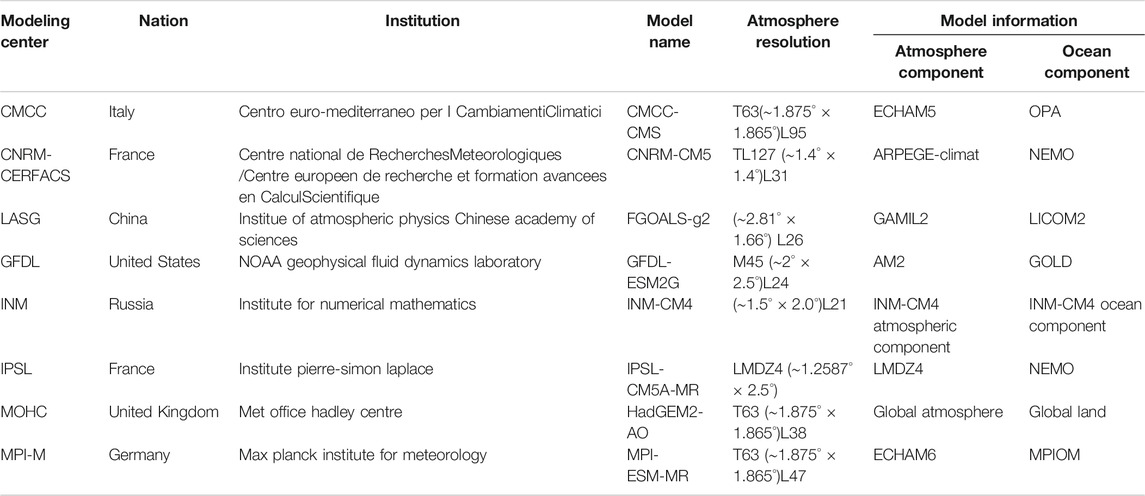
TABLE 1. Information about the CMIP5 climate models.

To uncover the geographical heterogeneity of DFA for SST in the oceans, we divided the oceans into 12 ocean basins (Table 2 and Figure 1). The 12 ocean basins are modified based on Chan et al (2015). We calculated the area-averaged DFA indexes in each ocean basin for NCEP and model output daily temperatures, then the area-averaged DFA indexes were compared to show the differences between the NCEP and model outputs.

TABLE 2. Names and coordinates for 12 ocean basins.

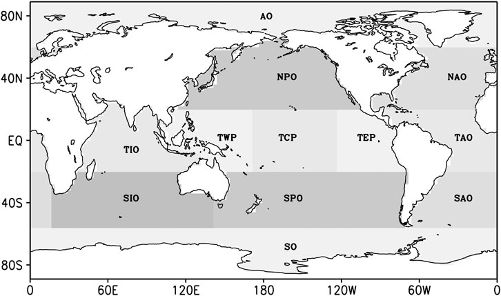
FIGURE 1. Divisions of the oceans.

Method

The DFA method can quantify LRC as index of power law exponent, namely, scaling exponent (Peng et al, 1994; Bunde et al., 2002, Bunde et al., 2005). DFA has been widely applied to study LRC in climate variabilities (Talkner and Weber, 2000; Kantelhardt et al., 2006; Gan et al., 2007; Jiang et al., 2013). For a giving time series, {X_i, i = 1, 2, …, N}, the departures x_i of X_i is calculated and cumulated to get the profile y(k).

Then profile y(k) is divided into n = Int (N/τ) non-overlapping segments of equal length τ. In each segment, a polynomial function is used to fit the local trend. If l-order polynomial function is used for the fitting, the order of DFA is l (DFA1 if l = 1, DFA2 if l = 2, etc.). Next, the local trend y_τ(k) is subtracted from profile y(k) in each segment, and the fluctuation function (F (τ)) of each segment is calculated by

A linear relationship on a log-log plot indicates the presence of the power law. In this case, fluctuations functions can be characterized by a scaling exponent α.

If α > 0.5, the time series {X_i, i = 1, 2, …, N} is positive long range correlation. If α = 0.5, the time series is uncorrelated. If α < 0.5, the time series has anti-persistent correlation. In this study, the DFA2 method is used to estimate the scaling exponent in a time series.

Long-Range Correlations of Daily Mean SST Over Ocean Simulated by CMIP5 Models

Characteristics of Daily mean SST Over Ocean

The equatorial Pacific Ocean (185°E, 0°) was selected as an example to study the long-range correlation characteristics of temperature over ocean. In the equatorial Pacific Ocean, the DFA value of NCEP daily temperature is 1.36, and the DFA values of the daily temperature simulated by the eight models vary between 0.91 and 1.41 (Figure 2A). In spring, the DFA value of NCEP’s daily temperature is 1.25. Except for FGOALS-G2, DFA values of the daily temperature simulated by the other seven models are all greater than 1.0, and that of GFDL-ESM2G is the largest, reaching 1.44 (Figure 2B). In summer, the DFA value of NCEP’s daily temperature is 1.23, slightly lower than that in spring. Except for FGOALS-G2 and INM-CM4, the DFA values of the other six models are all between one and 1.36 (Figure 2C). In autumn, the DFA value of NCEP's daily temperature is larger than these in spring and summer, reaching 1.31. Among the results of each model, the DFA value of daily temperature of GFDL-ESM2 is the smallest, reaching 0.72, and the largest is IPSL-CM5A-MR, reaching 1.41 (Figure 2D). In winter, the DFA value of NCEP's daily temperature is 1.35. Except for INM-CM4, the DFA values of the remaining seven models are all greater than 1, in which the maximum is1.47 of GFDL-ESM2G (Figure 2E).

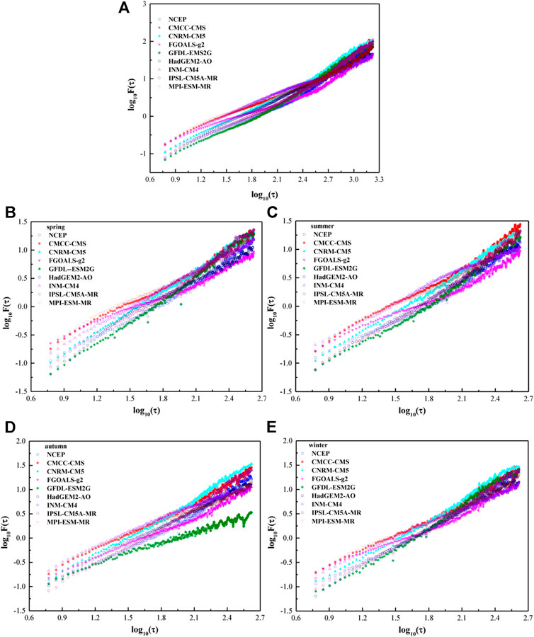
FIGURE 2. The DFA2 results of daily mean SST from NCEP and CMIP5 models at the point of (185°E, 0°) for (A) year, (B) spring, (C) summer, (D) autumn, and (E) winter.

Figure 3 shows that the DFA value of the daily temperature in this area over the years is larger than that of the four seasons, and the seasonal variation of the DFA value is not large, but the DFA value is smaller in spring and summer than that in autumn and winter. Except for GFDL-ESM2G, INM-CM4, and HadGEM2-AO, the seasonal changes of DFA values of the other models are close to NCEP data.

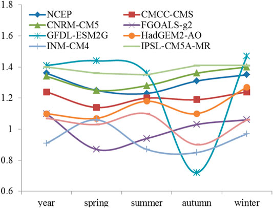
FIGURE 3. The DFA2 indexes of daily mean SST from NCEP and CMIP5 models at the point of (185°E, 0°) for year and all four seasons.

On the annual time scale, the median performance errors between the DFA values of the global daily mean SST simulated by CMCC-CMS, CNRM-CM5, HadGEM2-AO, and MPI-ESM-MR and those of the NCEP do not exceed ±0.01, while the median performance errors of INM-CM4 and FGOALS-g2 exceed −0.05 (Figure 4A). From the 5–95% error range of each model, the error margins of CMCC-CMS, GFDL-ESM2G, HadGEM2-AO and IPSL-CM5A-MR are less than 0.3, while those of the remaining four models are above 0.3, in which the maximum is 0.47 of INM-CM4. In spring, the median performance errors of CMCC-CMS, GFDL-ESM2G, IPSL-CM5A-MR and MPI-ESM-MR do not exceed ±0.01, and that of INM-CM4 exceeds −0.08 (Figure 4B). From the 5–95% error range of each model, the error margins of GFDL-ESM2G and HadGEM2-AO are the minimum, reaching 0.28, while the maximum is 0.37 of MPI-ESM-MR, and those of the other models are between 0.31 and 0.36. In summer, the median performance errors of CMCC-CMS, GFDL-ESM2G and MPI-ESM-MR are no more than ±0.01, that of INM-CM4 is -0.07, and those of the rest models are between ±0.01 and 0.06 (Figure 4C). From the 5–95% error range, the error margins of CNRM-CM5, GFDL-ESM2G, HadGEM2-AO and IPSL-CM5A-MR are the minimum, reaching 0.31, while the maximum is 0.45 of FGOALS-g2, and those of the rest are between 0.32 and 0.38. In autumn, the median performance errors of IPSL-CM5A-MR and MPI-ESM-MR are less than ±0.01, while that of INM-CM4 exceeds −0.07, and those of other models are between ±0.01 and 0.03 (Figure 4D). From the 5–95% error range, the minimum error margin is 0.25 of IPSL-CM5A-MR, while the maximum is 0.46 of INM-CM4, and those of the rest are between 0.26 and 0.4. In winter, the median performance errors of CMCC-CMS and GFDL-ESM2G are less than ±0.01, while that of FGOALS-g2 is −0.05, and those of the rest models are between ±0.01 and 0.04 (Figure 4E). From the 5–95% error range, the minimum error margin is 0.3 of IPSL-CM5A-MR, while the maximum is 0.46 of MPI-ESM-MR, and those of the rest are between 0.33 and 0.45.

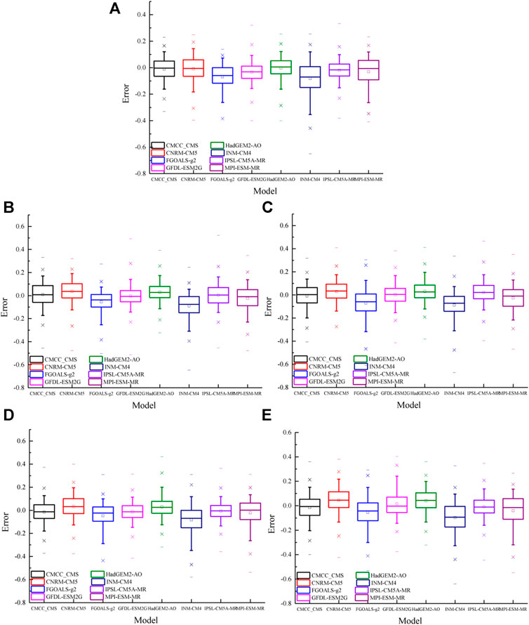
FIGURE 4. Box charts of the errors of DFA values from CMIP5 models for (A) year, (B) spring, (C) summer, (D) autumn, and (E) winter.

Long-Range Correlation Characteristics of Daily Mean SST in Various Regions of the Ocean

The zonal average value of the NCEP daily mean SST DFA index over the years shows that the DFA value is small in mid-high latitudes and large in tropical areas (Figure 5A), which decreases rapidly from the equator to the north and south direction. The zonal average DFA index exceeds 1.1 near the equator and decreases to 0.6 near the high latitudes of the southern and northern hemispheres. The DFA index of daily mean SST simulated by the eight models also shows similar characteristics of variation with the latitude, but the DFA values of the models in tropical regions are all smaller than the NCEP values, with large differences between the models. The zonal changes of DFA index in INM-CM4, MPI-ESM-MR and FGOALS-g2 models are smaller than NCEP. The minimum correlation coefficient between the INM-CM4 zonal average DFA value and the NCEP value is 0.78, and those of the other models are all above 0.9, in which the maximum correlation coefficient is 0.98 of IPSL-CM5A-MR.

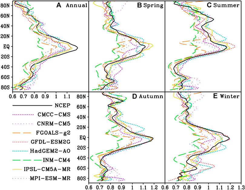
FIGURE 5. The zonal average distribution of the DFA index of NCEP and eight models of daily mean SST (A) year, (B) spring, (C) summer, (D) autumn, (E) winter.

In spring of the northern hemisphere, the zonal average value of the DFA index for NCEP daily mean SST is symmetrically distributed in the northern and southern hemispheres. DFA index of the tropical area is above 0.9, of which the equatorial area exceeds 1.1, and the mid-high latitude of the northern hemisphere is generally between 0.8 and 0.9, while that of the mid-high latitudes of the southern hemisphere is between 0.7 and 0.8 (Figure 5B). In the extratropical areas of the northern hemisphere, the zonal average DFA index changes slightly with latitudes, while that of the extratropical areas of the southern hemisphere increases slightly around 60°S, and then continues to decrease. The meridional changes of DFA index of INM-CM4, MPI-ESM-MR and FGOALS-g2 models are small. The zonal average DFA value of HadGEM2-AO has two peaks in the area outside the equator. The DFA values of GFDL-ESM2G and IPSL-CM5A-MR near the equator are larger than the NCEP values. The minimum correlation coefficient between the zonal average DFA index of INM-CM4 and MPI-ESM-MR and NCEP is 0.76, while those of the rest models are above 0.8, in which the maximum correlation coefficient is 0.97 of GFDL-ESM2G.

In summer of the northern hemisphere, the zonal average value of the NCEP daily temperature DFA index is still the largest near the equator, but the DFA value in the northern hemisphere is obviously larger than that in the southern hemisphere (Figure 5C). The zonal average DFA value displays a peak around 60°N in the northern hemisphere, reaching about 1.1, and then decreases toward higher latitudes rapidly. In the southern hemisphere, the zonal average DFA index rapidly decreases from the equator to around 40°S to a minimum of 0.7, and then goes up with the increase of latitudes. The zonal average DFA values of the eight models can all reflect the characteristic that the DFA value of the northern hemisphere is larger than that of the southern hemisphere. The zonal average DFA values of INM-CM4 and FGOALS-g2 do not reach a peak near the equator. The minimum correlation coefficient is 0.78 between the zonal average DFA index of FGOALS-g2 and NCEP, while those of the rest models are above 0.88, in which the maximum correlation coefficient is 0.96 of HadGEM2-AO.

In autumn of the northern hemisphere, the zonal average value of the DFA index for NCEP daily mean SST is symmetrically distributed in the northern and southern hemispheres, reaching a peak close to 1.2 near the equator, two small peaks near 50°N and 70°N in the northern hemisphere, and a smaller peak in 60°S in the southern hemisphere and then decreases towards higher latitudes (Figure 5D). The eight models can all reflect the characteristics that the zonal average DFA value is the largest near the equator, and the distribution in the northern and southern hemispheres is relatively symmetric. The zonal average DFA indices of INM-CM4, FGOALS-g2, and CMCC-CMS models vary little with latitudes and are significantly smaller than the NCEP value in tropical regions. The DFA value of HadGEM2-AO has a large peak near 20°N in the northern hemisphere. The minimum correlation coefficient between the zonal average DFA value of INM-CM4 and the NCEP value is 0.64, while those of the other models are all above 0.81, among which the correlation coefficients of GFDL-ESM2G and IPSL-CM5A-MR are up to 0.97.

In winter of the northern hemisphere, the zonal average value of the DFA index for NCEP daily mean SST is greater in the southern hemisphere than that in the northern hemisphere, and the peak still appears near the equator, reaching about 1.2. The DFA index of the northern hemisphere drops sharply to 0.8 from the equator to 30°N, then slowly decreases towards mid-high latitudes, and to about 0.7 near the north pole. The DFA index of the southern hemisphere decreases rapidly to about 0.7 from the equator to high latitudes (Figure 5E). The zonal average DFA index of the INM-CM4 and FGOALS-g2 models varies slightly with latitudes and is smaller than the NCEP value in tropical regions. Except that the correlation coefficient of zonal average DFA value and the NCEP value of HadGEM2-aO and IPSL-CM5A-MR exceeds 0.9, the correlation coefficients of the rest models are all less than 0.9, in which the minimum value is 0.72 of INM-CM4.

In general, the zonal average value of the DFA index for NCEP daily mean SST is the largest near the equator and smaller at mid-high latitudes, with obvious seasonal changing pattern. The variation range of the zonal average DFA value of INM-CM4 and FGOALS-g2 is smaller than the NCEP value, and the correlation coefficient with NCEP is relatively lower, while that of IPSL-CM5A-MR and HadGEM2-AO is closer to the NCEP value, with similar variation characteristics with latitudes.

Judging from the DFA value for daily mean SST of each region, the difference between the models and the DFA value of the NCEP is large in tropical regions. Among them, the tropical Central and Eastern Pacific has the largest difference, while that in middle and high latitudes is relatively small, generally less than ±0.1 (Figure 6A). In the North Atlantic (NAO), the simulated DFA values of the eight models have an error of less than ±0.05; in the Southern Ocean and the South Atlantic (SO and SAO), one model has an error of more than ±0.05. The errors of INM-CM4 and FGOALS-g2 are larger than those of other models.

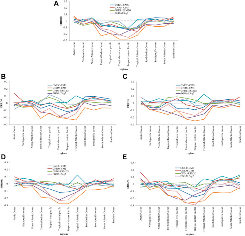
FIGURE 6. Differences between the DFA index of daily mean SST and the NCEP value in each region simulated by eight models, (A) throughout the year, (B) spring, (C) summer, (D) autumn, (E) winter.

In spring, the difference between the simulated daily mean SST DFA value and NCEP is still large in tropical regions, but the error in the mid-high latitudes of the northern hemisphere is significantly smaller than that in other parts of the world (Figure 6B). In the North Pacific (NPO) and North Atlantic (NAO), there is one model whose error is greater than ±0.05. In the Arctic Ocean (AO) and Southern Ocean (SO), there are two models whose errors exceed ±0.05. For Tropical Eastern Pacific (TEP), only HadGEM2-AO and IPSL-CM5A-MR have errors of less than ±0.05. The errors of INM-CM4, FGOALS-g2, and MPI-ESM-MR are larger than those of other models.

In summer, the difference between the DFA and NCEP values of most models is still larger in the tropics and smaller in the southern hemisphere (Figure 6C). The errors of all models in the South Indian Ocean (SIO) are all within ±0.05, and only one model has an error exceeding ±0.05 in the South Pacific (SPO). For the Arctic Ocean (AO), South Atlantic (SAO) and Southern Ocean (SO), only two models have an error exceeding ±0.05. In the tropical western Pacific (TWP), only HadGEM2-AO and IPSL-CM5A-MR have an error less than ±0.05.

In autumn, the error between the models’ DFA values and the NCEP values is larger in tropical regions, but smaller in mid-high latitudes in the northern and southern hemispheres (Figure 6D). In the North Atlantic (NAO), South Atlantic (SAO) and Southern Ocean (SO), the simulation error of only one model does not exceed ±0.05. In the North Pacific (NPO), Tropical Indian Ocean (TIO), South Indian Ocean (SIO) and South Pacific (SPO), there are two models with an error of more than ±0.05. In the tropical Atlantic, only GFDL-ESM2G and IPSL-CM5A-MRhave an error less than ±0.05.

In winter, the difference between the models’ DFA values and NCEP values is larger in the tropics, but smaller in the mid-high latitudes of the northern hemisphere (Figure 6E). In the North Atlantic Ocean (NAO), the simulation errors of all models are less than ±0.05. In the North Pacific (NPO), only INM-CM4 has a simulation error greater than ±0.05. In the South Indian Ocean (SIO), only HadGEM2-AO and INM-CM4 have an error greater than ±0.05. In the Tropical Atlantic (TAO) and South Pacific (SPO), only two models have simulation errors less than ±0.05.

Long-Range Correlation Assessment of Daily Mean SST Over Ocean in Multiple Models

The NCEP global daily mean SST has long-range correlation characteristics in most parts of the world. The DFA value over the tropical ocean is generally between 0.9 and 1.3. The DTA value of daily mean SST over the tropical Central and Eastern Pacific is above 1.3, and that of the mid-high latitudes is relatively small, in which that in the high latitudes of the northern hemisphere is below 0.7 (Figure 7A). Compared with the NCEP values, the DFA values of CMCC-CMS, CNRM-CM5, HadGEM2-AO and MPI-ESM-MR are smaller in the tropics, while the NCEP values are close to or larger than those in the tropics (Figure 7B,C,F,I). The DFA values of FGOALS-g2 and INM-CM4 are relatively small in most regions of the world except in the Arctic Ocean (Figure 7D,G). The DFA values of GFDL-ESM2G and IPSL-CM5A-MR are larger in some parts of the tropical western Pacific and mid-high latitudes in the southern hemisphere, while those in the rest of the world are close to or smaller than NCEP values (Figure 7H).

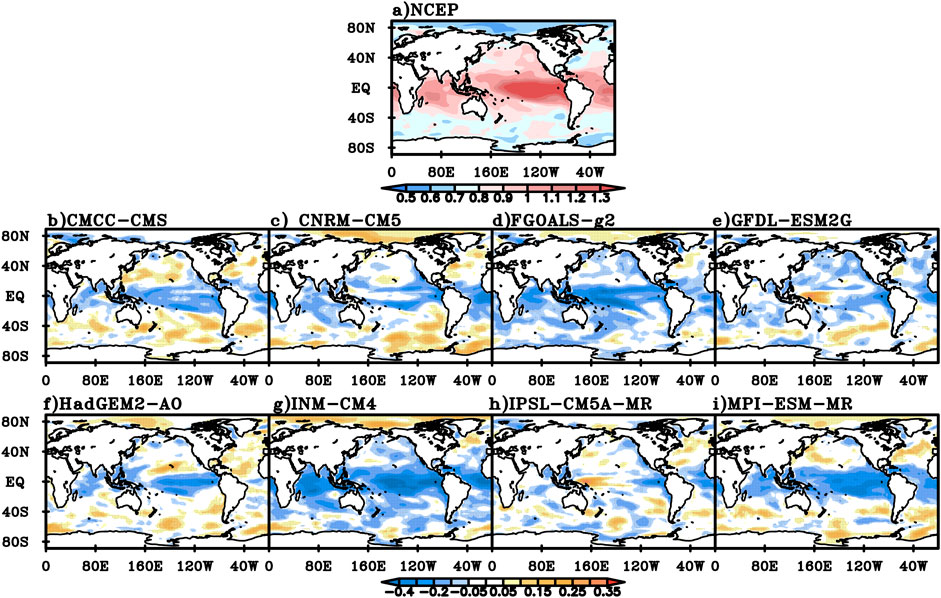
FIGURE 7. The DFA index for NCEP daily mean SST over the years (A) and the difference between the DFA index for daily mean SST simulated in the eight models and NCEP value (B) CMCC-CMS, (C) CNRM-CM5, (D) FGOALS-g2, (E) GFDL-ESM2G, (F) HadGEM-AO, (G) INM-CM4, (H) IPSL-CM5A-MR, (I) MPI-ESM-MR.

In spring, the DFA index for NCEP daily mean SST over the global ocean is generally above 0.7, and the DFA value in tropical area is generally between 0.9 and 1.2, while that over the equatorial Central and Eastern Pacific is above 1.2 (Figure 8A). Compared with the NCEP data, the DFA values for daily mean SST of CMCC-CMS and MPI-ESM-MR are mainly smaller near the equator, larger outside the tropics, and close to the NCEP value in the high latitudes of the northern hemisphere (Figure 8B,I). The DFA value of CNRM-CM5 is only small near the equator, large in the Arctic Ocean, and close to the NCEP value in the rest of the world (Figure 8C). The DFA value of FGOALS-g2 is close to or smaller than the NCEP value in most parts of the world, especially near the equator (Figure 8D). The DFA value of GFDL-ESM2G is larger in most parts of the tropical Pacific, tropical Indian Ocean and South Atlantic, and is close to or smaller than the NCEP value in the rest of the world (Figure 8E). For HadGEM2-AO, except that the DFA value is relatively small in the equatorial Central and Eastern Pacific, the value is close to or relatively larger than the NCEP value in most of the rest of the world (Figure 8F). The DFA value of INM-CM4 is smaller in most of the areas except the Arctic Ocean (Figure 8G). The DFA value of IPSL-CM5A-MR is smaller in the Arctic Ocean and the North Pacific, and is close to or larger than the NCEP value in the rest of the world (Figure 8H).

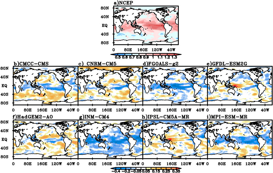
FIGURE 8. The DFA index for NCEP spring daily mean SST (A) and the difference between the DFA index for daily mean SST simulated in the eight models and NCEP value (B) CMCC-CMS, (C) CNRM-CM5, (D) FGOALS-g2, (E) GFDL-ESM2G, (F) HadGEM-AO, (G) INM-CM4, (H) IPSL-CM5A-MR, (I) MPI-ESM-MR.

In summer, the DFA value of NCEP daily mean SST is generally below 0.9 at mid-high latitudes in the southern hemisphere and the Arctic Ocean, generally between 0.9 and 1.3 in tropical oceans and mid-high latitudes in the northern hemisphere, and above 1.3 in the equatorial Central and Eastern Pacific (Figure 9A). Compared with NCEP data, the DFA values for daily mean SST of the CMCC-CMS and MPI-ESM-MR models are smaller in the tropical Pacific, North Pacific, tropical Atlantic and North Atlantic, but close to or larger than the NCEP value in the rest of the world (Figure 9B,I). The DFA value of CNRM-CM5 is larger in parts of the Arctic Ocean and Southern Ocean, smaller in the equatorial ocean and close to the NCEP value in the rest of the world (Figure 9C). For FGOALS-g2 and INM-CM4, except that the DFA values are larger in the Arctic Ocean, the values are close to or smaller than the NCEP value in the rest areas, especially notably smaller in tropical regions (Figure 9D,G). For GFDL-ESM2G and HadGEM2-AO, the DFA values are larger over the tropical ocean, and close to or smaller than the NCEP value in the rest of the world (Figure 9E,F). The DFA value of IPSL-CM5A-MR is larger in the tropical Pacific and Arctic Ocean, and is close to or smaller than the NCEP value in the rest of the world (Figure 9H).

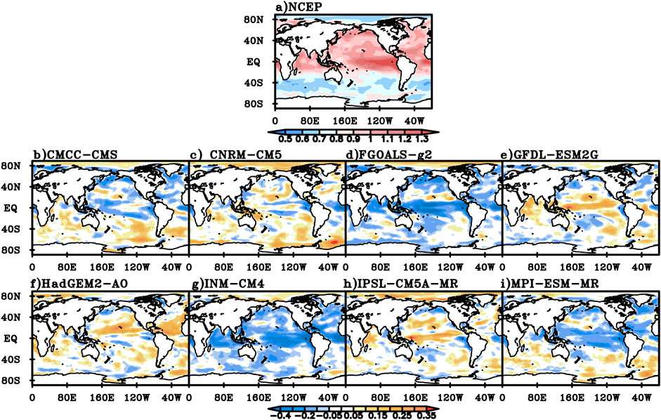
FIGURE 9. The DFA index for NCEP summer daily mean SST (A) and the difference between the DFA index for daily mean SST simulated in the eight models and NCEP value (B) CMCC-CMS, (C) CNRM-CM5, (D) FGOALS-g2, (E) GFDL-ESM2G, (F) HADGEM-AO, (G) INM-CM4, (H) IPSL-CM5A-MR, (I) MPI-ESM-MR.

In autumn, the DFA index for NCEP daily mean SST greater than 0.9 is mainly concentrated in tropical areas, while that in the Arctic Ocean and the southern hemisphere mid-high latitudes areas is generally below 0.7 (Figure 10A). Compared with the NCEP data, the DFA values of CMCC-CMS, FGOALS-g2 and MPI-ESM-MR models are larger over tropical oceans, but close to or smaller than the NCEP value in most other regions of the world (Figure 10B,D,I). The DFA values of CNRM-CM5 and GFDL-ESM2G are smaller in the equatorial Pacific, equatorial Atlantic, and parts of the South Indian Ocean, larger in parts of the Arctic Ocean and Southern Ocean, and close to the NCEP value in most parts of the world (Figure 10C,E). The DFA value of HadGEM2-AO is larger in the equatorial Pacific, the western and northern parts of the tropical Indian Ocean, and some parts of the Southern Ocean, and close to or larger than the NCEP value in the rest of the world, and is especially notably larger in the tropical North Pacific, the tropical North Atlantic and the Arctic Ocean (Figure 10F). The DFA value of INM-CM4 is only larger in the Arctic Ocean, but smaller in most parts of the world (Figure 10G). The DFA value of IPSL-CM5A-MR is smaller in parts of the South Indian Ocean, the tropical eastern Pacific, the South Atlantic, and the Southern Ocean, and is close to or larger than the NCEP value in most of the rest of the world (Figure 10I).

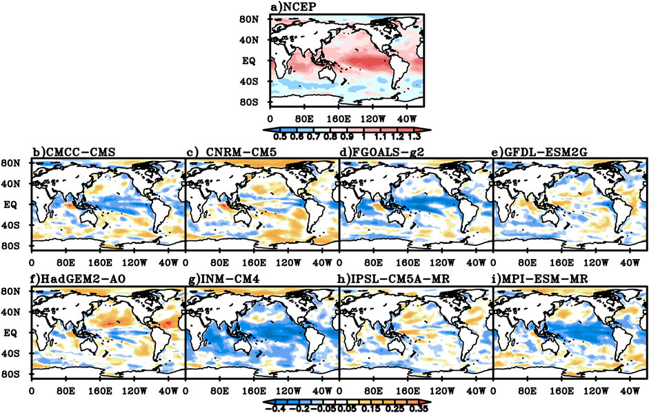
FIGURE 10. The DFA index for NCEP daily mean SST in autumn (A) and the difference between the DFA index for daily mean SST simulated in the eight models and NCEP value (B) CMCC-CMS, (C) CNRM-CM5, (D) FGOALS-g2, (E) GFDL-ESM2G, (F) HadGEM-AO, (G) INM-CM4, (H) IPSL-CM5A-MR, (I) MPI-ESM-MR.

In winter, the DFA index for NCEP daily mean SST is generally between 0.9 and 1.3 in tropical regions and the Southern Ocean, and that in the tropical Central and Eastern Pacific is generally above 1.3 (Figure 11A). Compared with the NCEP data, the DFA values of CMCC-CMS, FGOALS-g2, IPSL-CM5A-MR and MPI-ESM-MR models are smaller in tropical regions and parts of the Southern Ocean, but close to or larger than the NCEP value in the rest of the world (Figure 11B,D,H,I). The DFA value of CNRM-CM5 is smaller in the equatorial region, but larger in parts of the Arctic Ocean and Southern Ocean, and close to the NCEP value in most other parts of the world (Figure 11C). The DFA value of GFDL-ESM2G is close to or smaller than the NCEP value in the northern hemisphere, while close to or larger than the NCEP value in most parts of the southern hemisphere except the south Indian Ocean (Figure 11E). The DFA value of HadGEM2-AO is only smaller in parts of the tropical Pacific and North Pacific, and close to or larger than the NCEP value in most other parts of the world, of which the value in South Pacific and Southern Ocean is significantly larger (Figure 11F). The DFA value of INM-CM4 value is larger in the Arctic Ocean and smaller in most other parts of the world (Figure 11G).

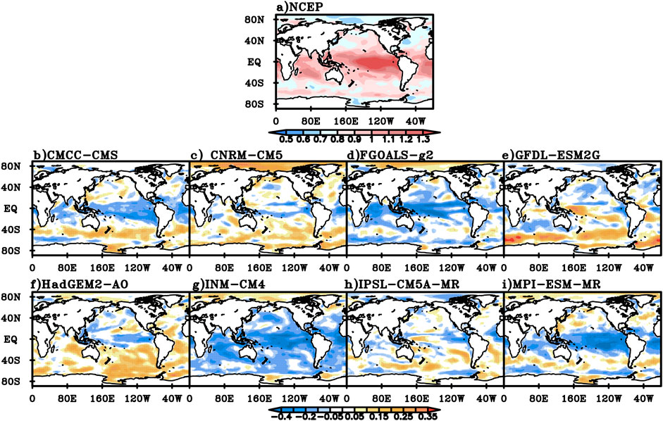
FIGURE 11. The DFA index for NCEP winter daily mean SST (A) and the difference between the DFA index for daily mean SST simulated in the eight models and NCEP value (B) CMCC-CMS, (C) CNRM-CM5, (D) FGOALS-g2, (E) GFDL-ESM2G, (F) HadGEM-AO, (G) INM-CM4, (H) IPSL-CM5A-MR, (I) MPI-ESM-MR.

Discussion and Conclusion

Based on NCEP data, the simulations of daily mean SST by eight CMIP5 models during 1960–2005 are evaluated using DFA method. The results of NCEP data showed that the daily mean SST in most regions of the ocean has long-range correlation characteristics. The DFA values of daily mean SST over ocean basins are large in the tropics while small in mid-high latitudes. The zonal average DFA values of IPSL-CM5A-MR and HadGEM2-AO had a meridional variation characteristic, which was close to NCEP. The regional average of the DFA values of eight models are all close to those of the NCEP data in North Atlantic, Southern Ocean, and North Pacific.

The DFA value of daily mean SST over the years showed that the DFA values of DAT is relatively large in tropical regions, especially in the equatorial Central and Eastern Pacific. In the view of the DFA bias of different models, there were fewer areas where the DFA bias exceeds ±0.05 for CNRM-CM5, HadGEM2-AO and ISPL-CM5A-MR. In spring, the DFA value of the NCEP DAT was generally above 0.7 over the global ocean, between 0.9 and 1.2 in tropical areas, and above 1.2 over the equatorial Central and Eastern Pacific. In the view of DFA bias, the performance of CNRM-CM5, GFDL-ESM2G, HadGEM2-AO and IPSL-CM5A-MR was better than other models. In summer, the DFA values of NCEP DAT was larger in the northern hemisphere than those in the southern hemisphere. The DFA values of CNRM-CM5, GFDL-ESM2G, HadGEM2-AO and ISPL-CM5A-MR are close to those of NCEP in most parts of the global ocean, indicating good performance. In autumn, the DFA values of NCEP DAT were generally above 0.9 in tropical regions and above 1.3 in the equatorial Central and Eastern Pacific. The DFA bias of CNRM-CM5, GFDL-ESM2G, and IPSL-CM5A-MR were relatively small in most regions of the global ocean. In winter, the DFA values of NCEP DAT were generally above 1.0 in tropical regions, while below 0.8 only in the Arctic Ocean and the North Atlantic. The performance of CNRM-CM5, FGAOLS-g2, and IPSL-CM5A-MR were good in most parts of the global ocean.

The LRC method has been widely used to verify the performance of climate models for the climate simulation (Zhao et al., 2017; He and Zhao, 2018). However, most of previous studies focus on the land surface air temperature, little research on sea surface temperature has been conducted. Therefore, some significant conclusions in this paper have been shown for the revelation of sea surface temperature simulation by climate models using LRC method. Although, it is important to make sure that the different sources of uncertainty are identified when using CMIP models to conduct climate projection. Future emissions, internal variability of the climate system and model response uncertainty are the three main sources of uncertainty in CMIP MME. Different responses to the same forcing can emerge due to different processes and feedbacks as well as due to the parametrization used in the different models (Zelinka et al., 2020). There are uncertainties exiting in the interpolation for outputs from CMIP models and the gauged data to 1.0° × 1.0°grids using the inverse distance weighting approach. Hence, the model weighting scheme for MME and dynamic downscaling method with more complete physical and dynamic processes will be adopted to conduct the region climate simulation and projection based on CMIP5/6 model output in the future, and it will significantly improve the reliability of simulations and projections. These will be the topic of our research in future.

Data Availability Statement

The original contributions presented in the study are included in the article/Supplementary Material, further inquiries can be directed to the corresponding author.

Author Contributions

SZ and WH conceived of the presented idea. XZ and TD carried out the implementation. XZ performed the calculations. All authors discussed the results and contributed to the final manuscript.

Funding

This work was funded by National Key R&D Program of China (2016YFA0602703), the National Natural Science Foundation of China (Grant No. 41775092, 41875120, and 41605069), the China Postdoctoral Science Foundation (Grant No. 2020M672942), the Fundamental Research Funds for the Central Universities from Sun Yat-Sen University (Grant No. 20lgzd06 and 19lgpy31).

Conflict of Interest

The authors declare that the research was conducted in the absence of any commercial or financial relationships that could be construed as a potential conflict of interest.

References

Alexander, L. V., and Arblaster, J. M. (2009). Assessing Trends in Observed and Modelled Climate Extremes over Australia in Relation to Future Projections. Int. J. Climatol. 29, 417–435. doi:10.1002/joc.1730
Alexander, L. V., Zhang, X., Peterson, T. C., Caesar, J., Gleason, B., Klein Tank, A. M. G., et al. (2006). Global Observed Changes in Daily Climate Extremes of Temperature and Precipitation. J. Geophys. Res. 111, D05109. doi:10.1029/2005JD006290
Blender, R., and Fraedrich, K. (2003). Long Time Memory in Global Warming Simulations. Geophys. Res. Lett. 30 (14), 1769. doi:10.1029/2003gl017666
Bunde, A., Eichner, J. F., Kantelhardt, J. F., and Havlin, S. (2005). Long-Term Memory: A Natural Mechanism for the Clustering of Extreme Events and Anomalous Residual Times in Climate Records. Phys. Rev. Lett. 94, 048701. doi:10.1103/physrevlett.94.048701
Bunde, A., and Havlin, S. (2002). Power-law Persistence in the Atmosphere and in the Oceans. Physica A: Stat. Mech. its Appl. 314, 15–24. doi:10.1016/s0378-4371(02)01050-6
Chan, D., and Wu, Q. (2015). Attributing Observed SST Trends and Subcontinental Land Warming to Anthropogenic Forcing during 1979-2005. J. Clim. 28, 3152–3170. doi:10.1175/jcli-d-14-00253.1
Gan, Z., Yan, Y., and Qi, Y. (2007). Scaling Analysis of the Sea Surface Temperature Anomaly in the South China Sea. J. Atmos. Ocean. Tech. 24, 681–687. doi:10.1175/jtech1981.1
Grose, M. R., Narseym, S., Delage, F., Dowdy, A. J., Bador, M., Boschat, G., et al. (2020). Insights from CMIP6 for Australia's Future Climate. Earth's Future 8 (5), e2019EF001469. doi:10.1029/2019EF001469
Gusain, A., Ghosh, S., and Karmakar, S. (2020). Added Value of CMIP6 over CMIP5 Models in Simulating Indian Summer Monsoon Rainfall. Atmos. Res. 232, 104680. doi:10.1016/j.atmosres.2019.104680
He, W. P., and Zhao, S. S. (2018). Assessment of the Quality of NCEP-2 and CFSR Reanalysis Daily Temperature in China Based on Long-Range Correlation. Clim. Dyn. 50, 493–505. doi:10.1007/s00382-017-3622-0
IPCC (2013). Climate Change 2013: The Physical Science Basis. Contribution of Working Group I to the Fifth Assessment Report of the Intergovernmental Panel on Climate Change. Cambridge, UK, and New York, NY: Cambridge University Press.
Ji, Z., and Kang, S. (2015). Evaluation of Extreme Climate Events Using a Regional Climate Model for China. Int. J. Climatol. 35, 888–902. doi:10.1002/joc.4024
Jiang, D., and Tian, Z. (2013). East Asian Monsoon Change for the 21st century: Results of CMIP3 and CMIP5 Models. Chin. Sci. Bull. 58, 1427–1435. doi:10.1007/s11434-012-5533-0
Jiang, L., Zhao, X., Li, N., Li, F., and Guo, Z. (2013). Different Multifractal Scaling of the 0 Cm Average Ground Surface Temperature of Four Representative Weather Stations over China. Adv. Meteorology 2013, 1–8. doi:10.1155/2013/341934
Kalnay, E., Kanamitsu, M., Kistler, R., Collins, W., Deaven, D., Gandin, L., et al. (1996). The NCEP/NCAR 40-year Reanalysis Project. Bull. Amer. Meteorol. Soc. 77, 437–471. doi:10.1175/1520-0477(1996)077<0437:tnyrp>2.0.co;2
Kanamitsu, M., Ebisuzaki, W., Woollen, J., Yang, S.-K., Hnilo, J. J., Fiorino, M., et al. (2002). NCEP-DOE AMIP-II Reanalysis (R-2). Bull Amer. Meteorol. Soc. 83, 1631–1643. doi:10.1175/bams-83-11-1631(2002)083<1631:nar>2.3.co;2
Kantelhardt, J. W., Koscielny-Bunde, E., Rybski, D., Braun, P., Bunde, A., and Havlin, S. (2006). Long-term Persistence and Multifractality of Precipitation and River Runoff Records. J. Geophys. Res. 111. doi:10.1029/2005JD005881
Kharin, V. V., Zwiers, F. W., Zhang, X., and Hegerl, G. C. (2007). Changes in Temperature and Precipitation Extremes in the IPCC Ensemble of Global Coupled Model Simulations. J. Clim. 20, 1419–1444. doi:10.1175/jcli4066.1
Kharin, V. V., Zwiers, F. W., Zhang, X., and Wehner, M. (2013). Changes in Temperature and Precipitation Extremes in the CMIP5 Ensemble. Climatic Change 119 (2), 345–357. doi:10.1007/s10584-013-0705-8
Koscielny-Bunde, E., Roman, H. E., Bunde, A., Havlin, S., and Schellnhuber, H. J. (1998). Long-range Power-Law Correlations in Local Daily Temperature Fluctuation. Philosophical Mag. B 77 (5), 1331–1340.
Koscielny-Bunde, E., Bunde, A., Havlin, S., and Goldreich, Y. (1996). Analysis of Daily Temperature Fluctuations. Physica A: Stat. Mech. its Appl. 231 (4), 393–396. doi:10.1016/0378-4371(96)00187-2
Kruger, A. C., and Sekele, S. S. (2013). Trends in Extreme Temperature Indices in South Africa: 1962-2009. Int. J. Climatol. 33, 661–676. doi:10.1002/joc.3455
Peng, C.-K., Buldyrev, S. V., Havlin, S., Simons, M., Stanley, H. E., and Goldberger, A. L. (1994). Mosaic Organization of DNA Nucleotides. Phys. Rev. E 49, 1685–1689. doi:10.1103/physreve.49.1685
Prinn, R. G. (2012). Development and Application of Earth System Models,Proc. Natl. Acad. Sci. 110. Supplement_1 3673–3680. doi:10.1073/pnas.1107470109pnas.1107470109
Rusticucci, M. (2012). Observed and Simulated Variability of Extreme Temperature Events over South America. Atmos. Res. 106, 1–17. doi:10.1016/j.atmosres.2011.11.001
Sillmann, J., Kharin, V. V., Zwiers, F. W., Zhang, X., and Bronaugh, D. (2013). Climate Extremes Indices in the CMIP5 Multimodel Ensemble: Part 2. Future Climate Projections. J. Geophys. Res. Atmos. 118, 2473–2493. doi:10.1002/jgrd.50188
Talkner, P., and Weber, R. O. (2000). Power Spectrum and Detrended Fluctuation Analysis: Application to Daily Temperatures. Phys. Rev. E 62 (1), 150–160. doi:10.1103/physreve.62.150
Taylor, K. E., Stouffer, R. J., and Meehl, G. A. (2012). An Overview of CMIP5 and the experiment Design. Bull. Amer. Meteorol. Soc. 93, 485–498. doi:10.1175/bams-d-11-00094.1
Tebaldi, C., Smith, R. L., Nychka, D., and Mearns, L. O. (2005). Quantifying Uncertainty in Projections of Regional Climate Change: a Bayesian Approach to the Analysis of Multimodel Ensembles. J. Clim. 18, 1524–1540. doi:10.1175/jcli3363.1
Wang, Y., Zhou, B., Qin, D., Wu, J., Gao, R., and Song, L. (2017). Changes in Mean and Extreme Temperature and Precipitation over the Arid Region of Northwestern China: Observation and Projection. Adv. Atmos. Sci. 34 (3), 287–305. doi:10.1007/s00376-016-6160-5
Wei, M., and Qiao, F. (2016). Attribution Analysis for the Failure of CMIP5 Climate Models to Simulate the Recent Global Warming Hiatus. Sci. China Earth Sci. 60 (2), 397–408. doi:10.1007/s11430-015-5465-y
Zelinka, M. D., Myers, T. A., McCoy, D. T., Po‐Chedley, S., Caldwell, P. M., Ceppi, P., et al. (2020). Causes of Higher Climate Sensitivity in CMIP6 Models. Geophys. Res. Lett. 47, 1–12.Z. doi:10.1029/2019gl085782
Zeng, Q. C., Zhou, G. Q., Pu, Y. F., Chen, W., Li, R. F., Liao, H., et al. (2008). Research on the Earth System Dynamic Model and Some Related Numerical Simulations. Chin. J. Atmos. Sci. 32 (4), 653–690. doi:10.3724/SP.J.1148.2008.00288
Zhao, S. S., and He, W. P. (2014). Performance Evaluation of Chinese Air Temperature Simulated by Beijing Climate Center Climate System Model on the Basis of the Long-Range Correlation. Acta Physica Sinica 63 (20), 209201
Zhao, S. S., He, W. P., and Jiang, Y. (2017). Evaluation of NCEP-2 and CFSR Reanalysis Seasonal Temperature Data in China Using Detrended Fluctuation Analysis. Int. J. Climatol 38, 252–263. doi:10.1002/joc.5173
Zhao, Z. C., Luo, Y., and Huang, J. B. (2013). A Review on Evaluation Methods of Climate Modeling[J]. Progressus Inquisitiones de Mutatione Climatis 9 (1), 1–8.
Zhou, B., Wen, Q. H., Xu, Y., Song, L., and Zhang, X. (2014). Projected Changes in Temperature and Precipitation Extremes in china by the Cmip5 Multimodel Ensembles. J. Clim. 27, 6591–6611. doi:10.1175/jcli-d-13-00761.1
Keywords: detrended fluctuation analysis, long-range correlation, CMIP5, NCEP, SST
Citation: Zhu X, Dong T, Zhao S and He W (2021) A Comparison of Global Surface Air Temperature Over the Oceans Between CMIP5 Models and NCEP Reanalysis. Front. Environ. Sci. 9:656779. doi: 10.3389/fenvs.2021.656779
Received: 21 January 2021; Accepted: 06 May 2021;
Published: 21 May 2021.
Edited by:
Boyin Huang, National Oceanic and Atmospheric Administration, United StatesReviewed by:
Fei Xie, Beijing Normal University, ChinaRuiqiang Ding, Beijing Normal University, China
Copyright © 2021 Zhu, Dong, Zhao and He. This is an open-access article distributed under the terms of the Creative Commons Attribution License (CC BY). The use, distribution or reproduction in other forums is permitted, provided the original author(s) and the copyright owner(s) are credited and that the original publication in this journal is cited, in accordance with accepted academic practice. No use, distribution or reproduction is permitted which does not comply with these terms.
*Correspondence: Shanshan Zhao, zhaoss@cma.gov.cn