
Debris Flow and Rockslide Analysis with Advanced Photogrammetry Techniques Based on High-Resolution RPAS Data. Ponte Formazza Case Study (NW Alps)

 ,
,  , , ,
, , ,
Abstract
:
1. Introduction
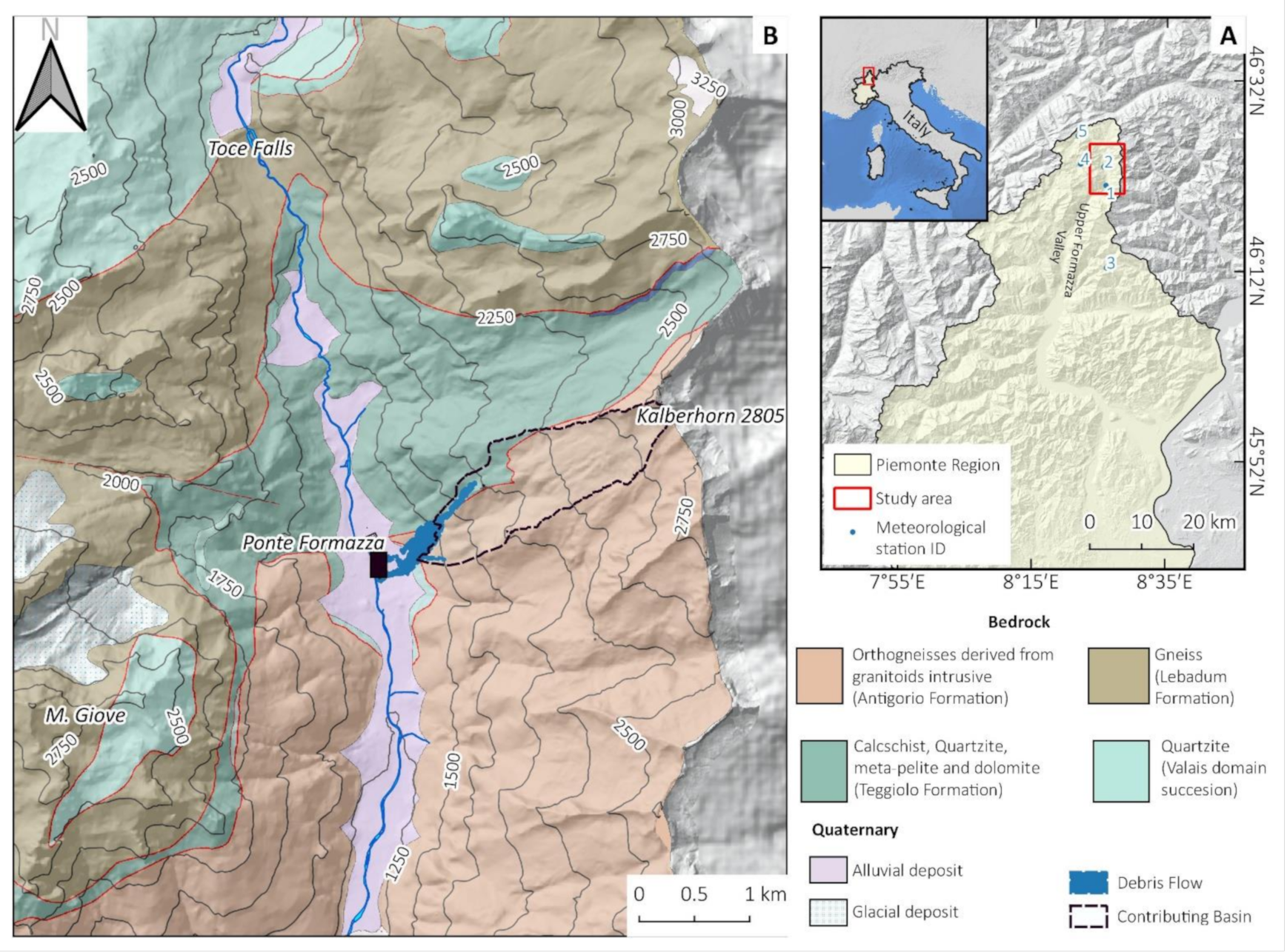
2. Study Area
2.1. Geological and Geomorphological Settings
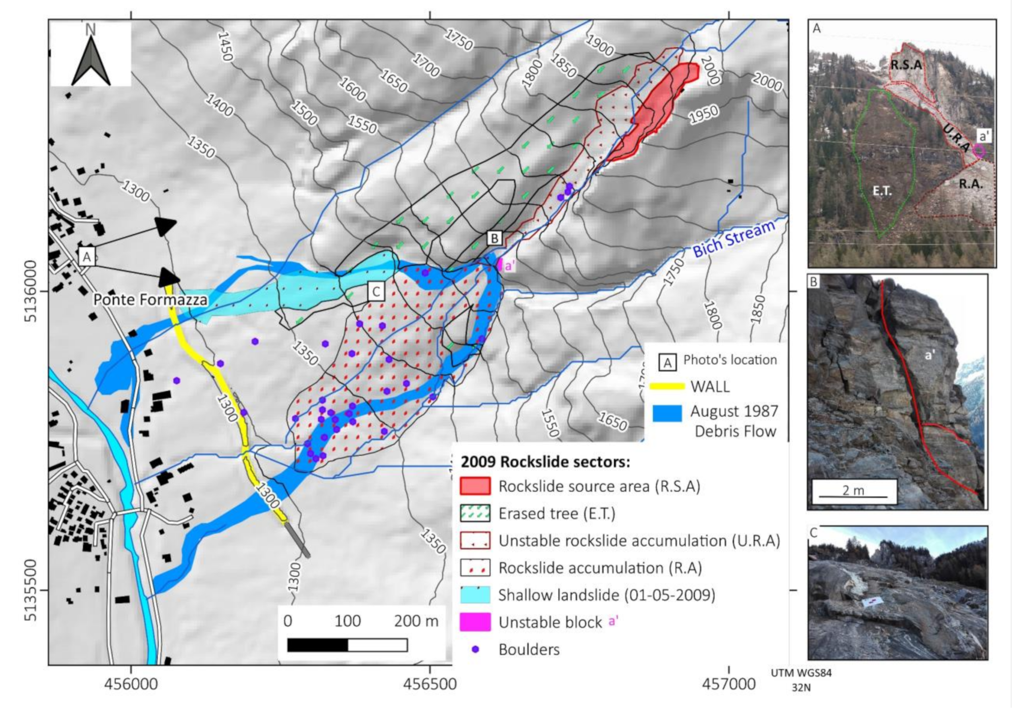
2.2. Previous Events: April 2009 Rockslide
3. Materials and Methods
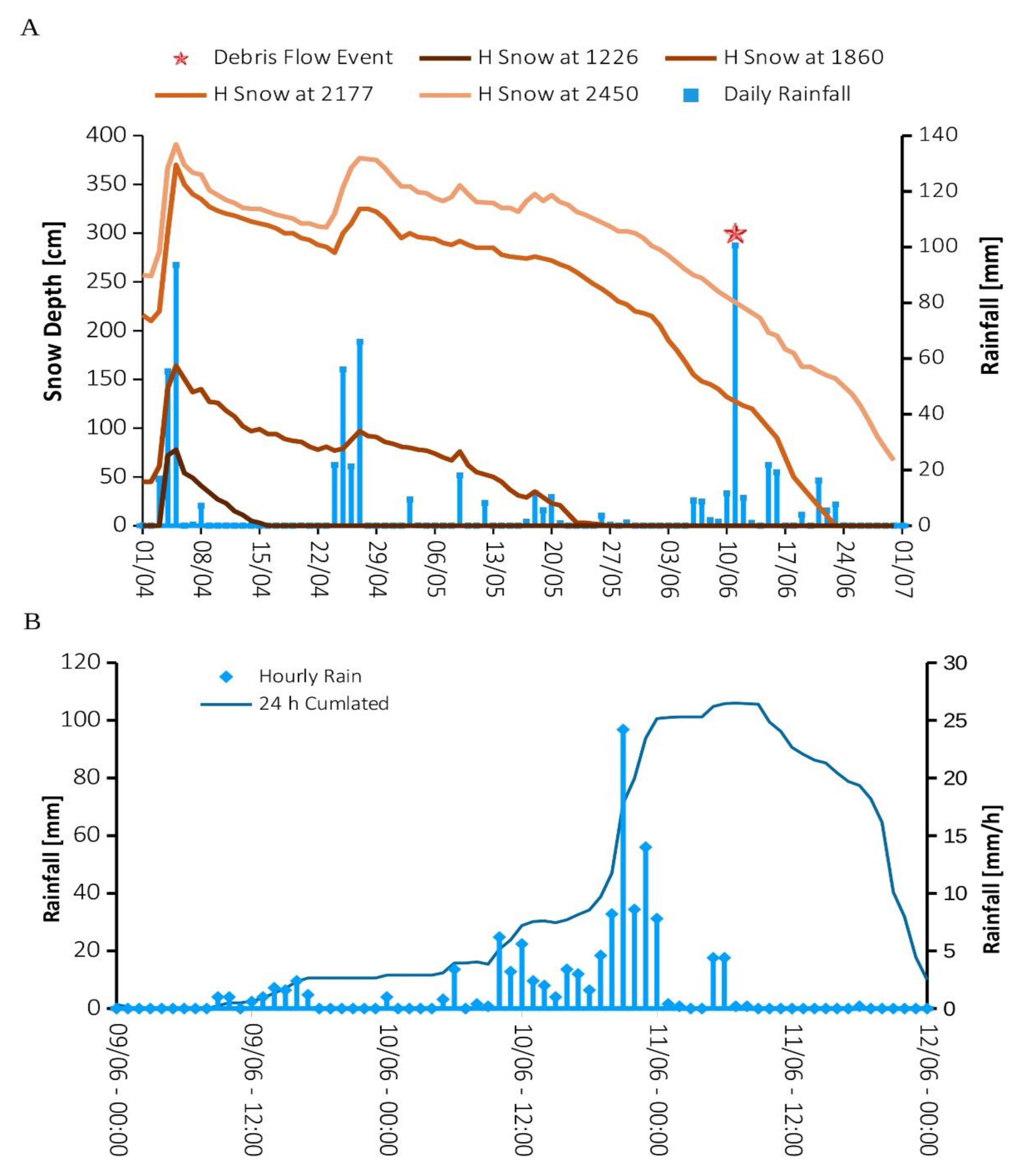
3.1. Meteorological Data
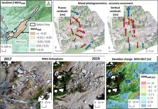
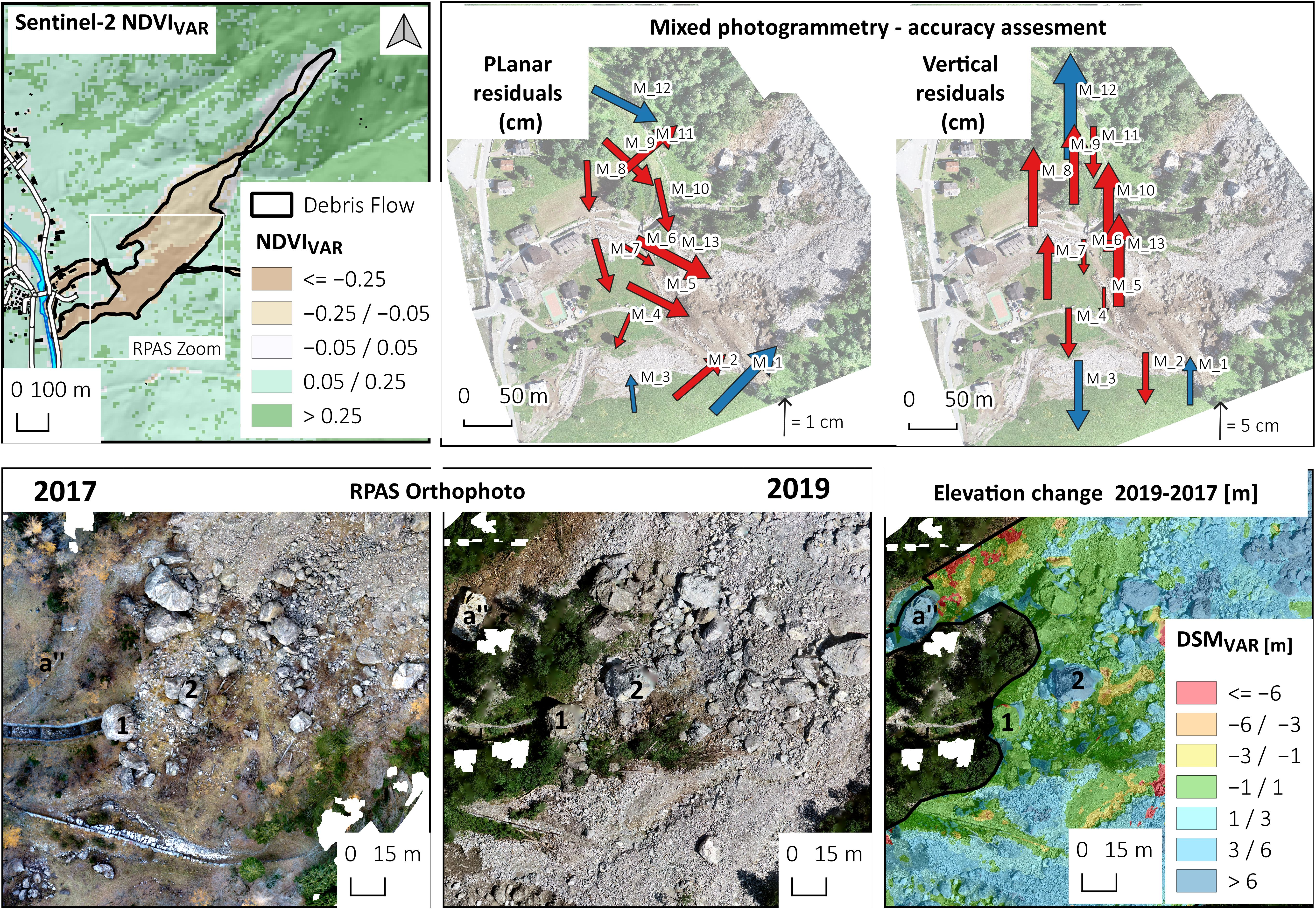
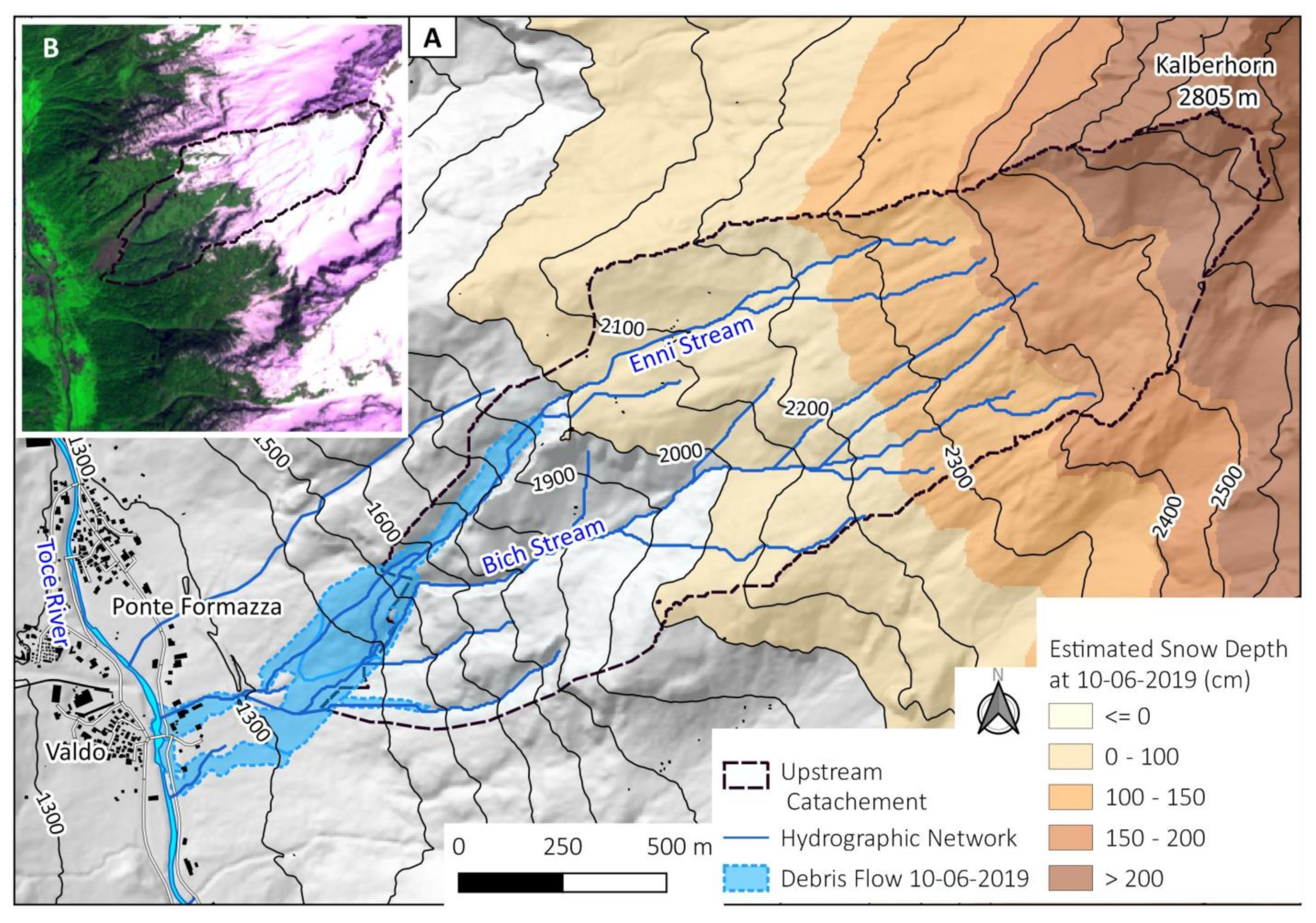
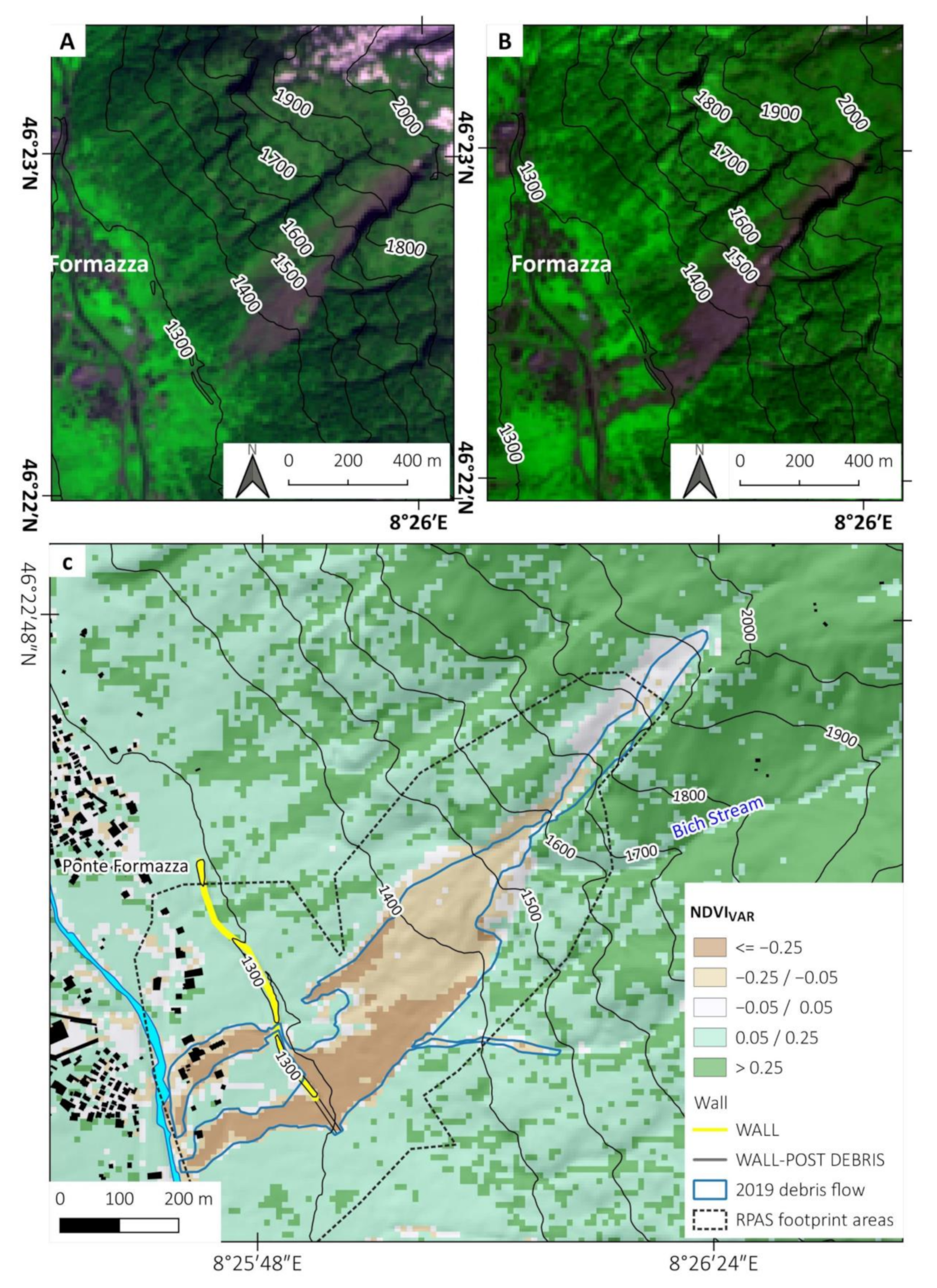
3.2. Low-resolution Mapping and Snow Coverage Estimation
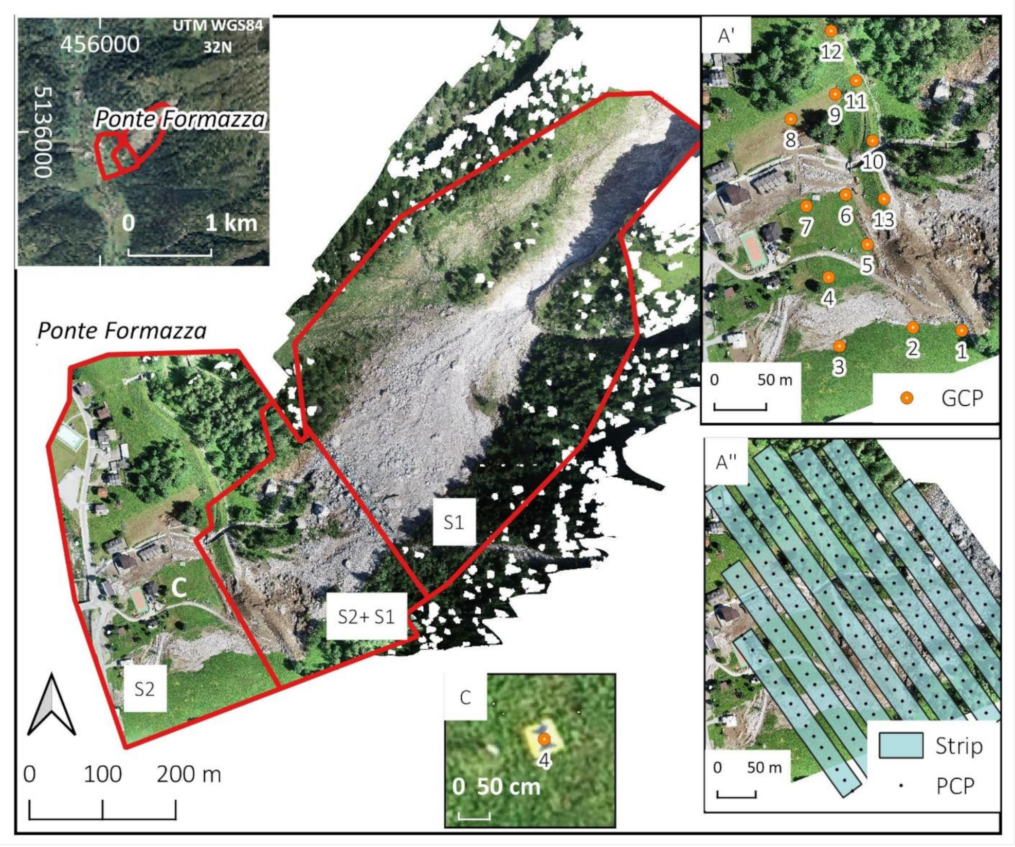
3.3. High-Resolution Mapping Strategy
3.4. Mapping with RPAS: Processing Strategies in Emergency Cases
Traditional, Direct and Mixed Photogrammetry Techniques Using an SfM Software
- Finding homologous points, named key points, in all photograms.
- Performing the relative orientation of the images (also named camera frames orientation).
- Performing the absolute orientation of the block of photograms with some measures (GCPs and/or PCs). This part is classically named “Aerial Triangulation” (AT).
- Building the dense cloud.
- Building of mesh and texture.
- Building of DSM, DTM, and Orthophoto.
- Traditional photogrammetry: Using Ground Control Points only (GCPs).
- Direct photogrammetry: the use of Projection Centre Points (PCPs).
- Mixed approach: the use of both PCPs and a variable number of GCPs (from one up to 13).
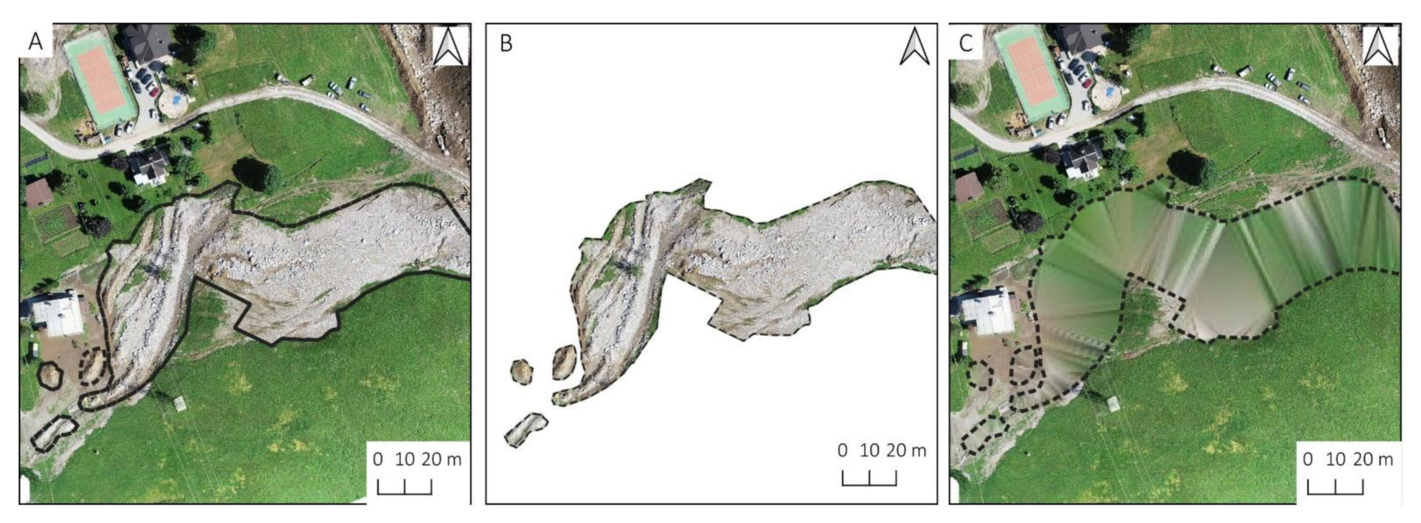
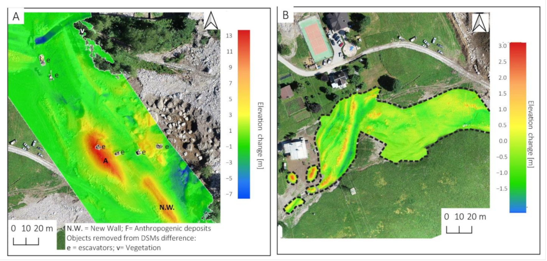
3.5. Volume Estimation and Geomorphological Mapping of the Debris Flow
- we first cut out from DSM the area covered by debris (Figure 4B);
- we proceeded to interpolate the clipped part to reconstruct the surface before the event (Figure 4C);
- we calculated the difference between the original raw DSM and the reconstructed DSM pre-event. This allowed us to estimate the volume also of this sector (see Figure 8A in the results).
4. Results
4.1. Meteorological Analysis of the 2019 Event
4.2. Low-Resolution Mapping
4.3. High-Resolution Mapping Results
4.3.1. SfM for DSM and Orthophoto Production
4.3.2. Accuracy Results in SfM Software for the Aerial Triangulation Cases
4.3.3. DSM and Volume Accuracy in the Lower Sector of Landslides
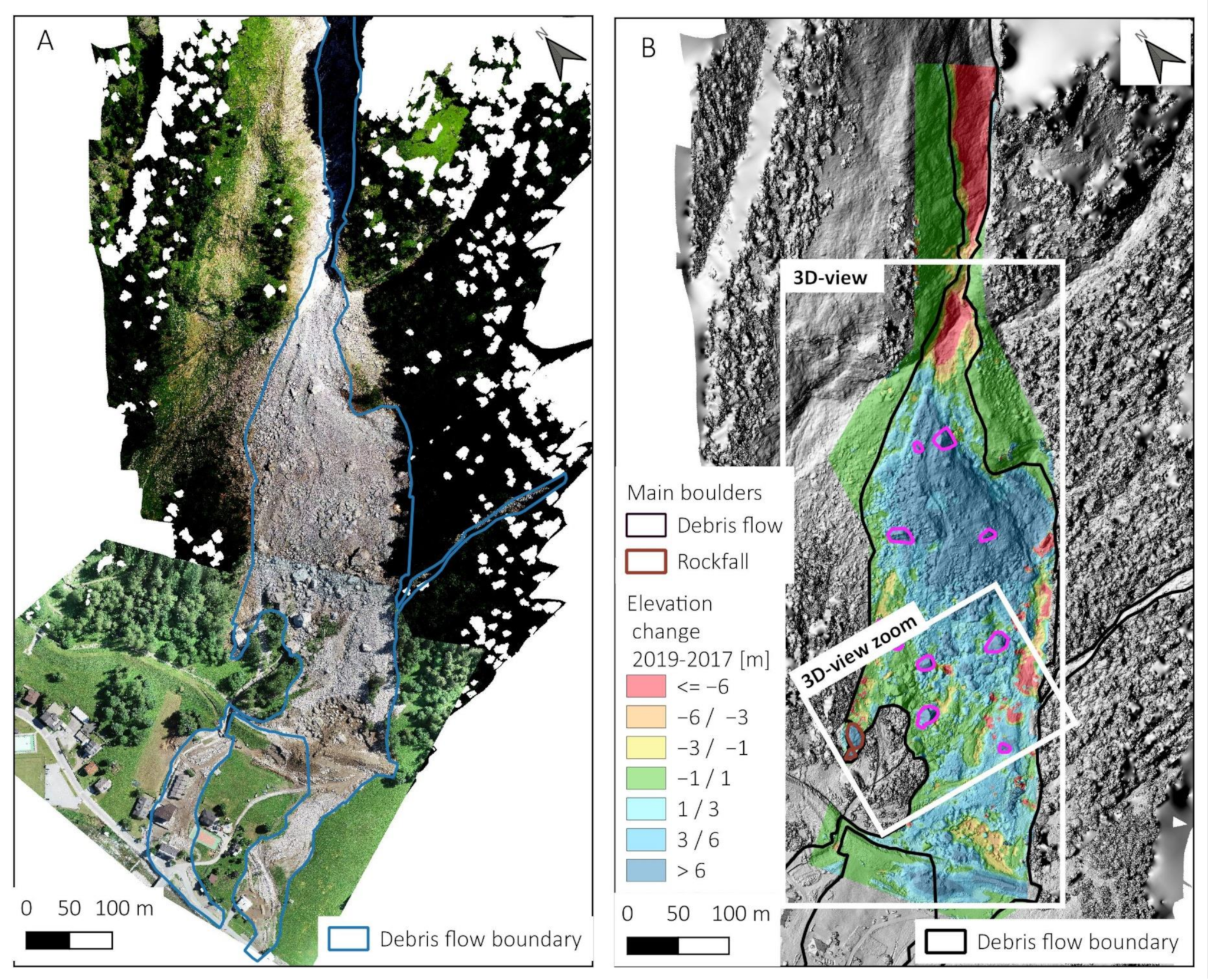
4.3.4. Rockslide and Debris Flow Volume Estimation and Mapping Based on SfM
4.4. Geomorphological Interpretation
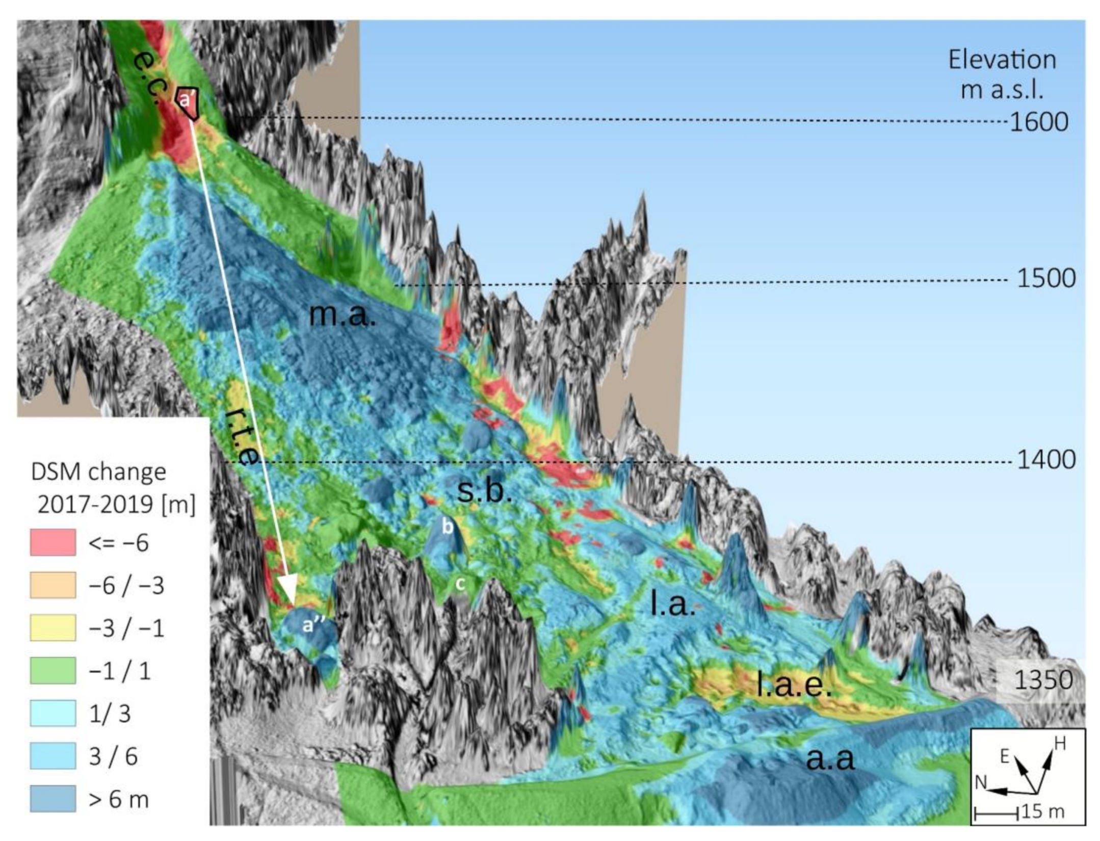
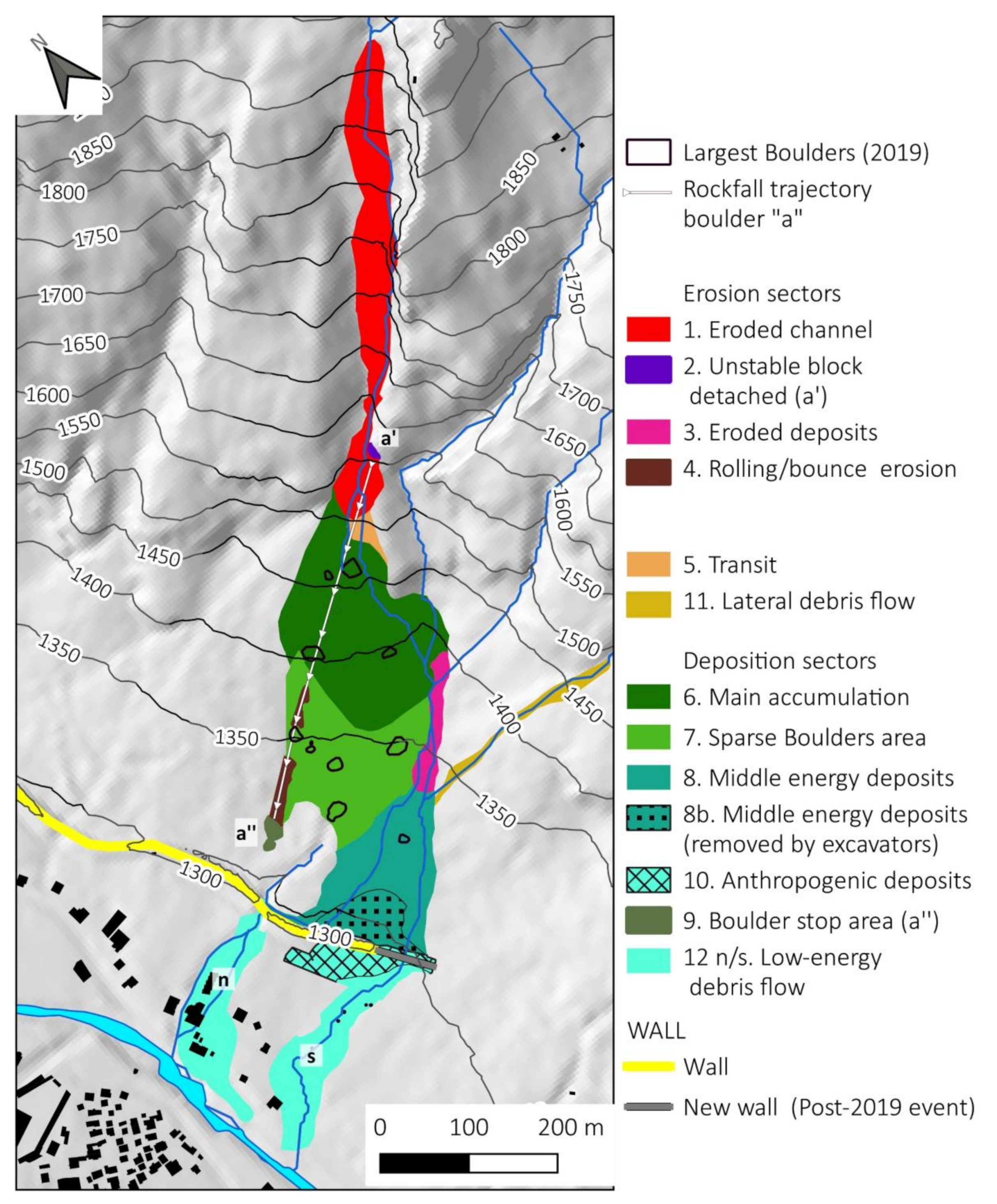
- Erosion sectors (red/violet colors in Figure 13). Here it is possible to find the eroded channel (1) (source of most of the material mobilized; the area of the detachment of the block a’) (2) and the erosion caused by its rolling and bounce (4 a/b); a small area of erosion (3) on the left side of the rockslide deposit related to debris flow action increased by the Bich stream.
- A small transit sector (5) where erosion and deposits are balanced (orange color in Figure 13). Another transit sector is the lateral debris flow (12) that increased the energy for the middle section of the slope.
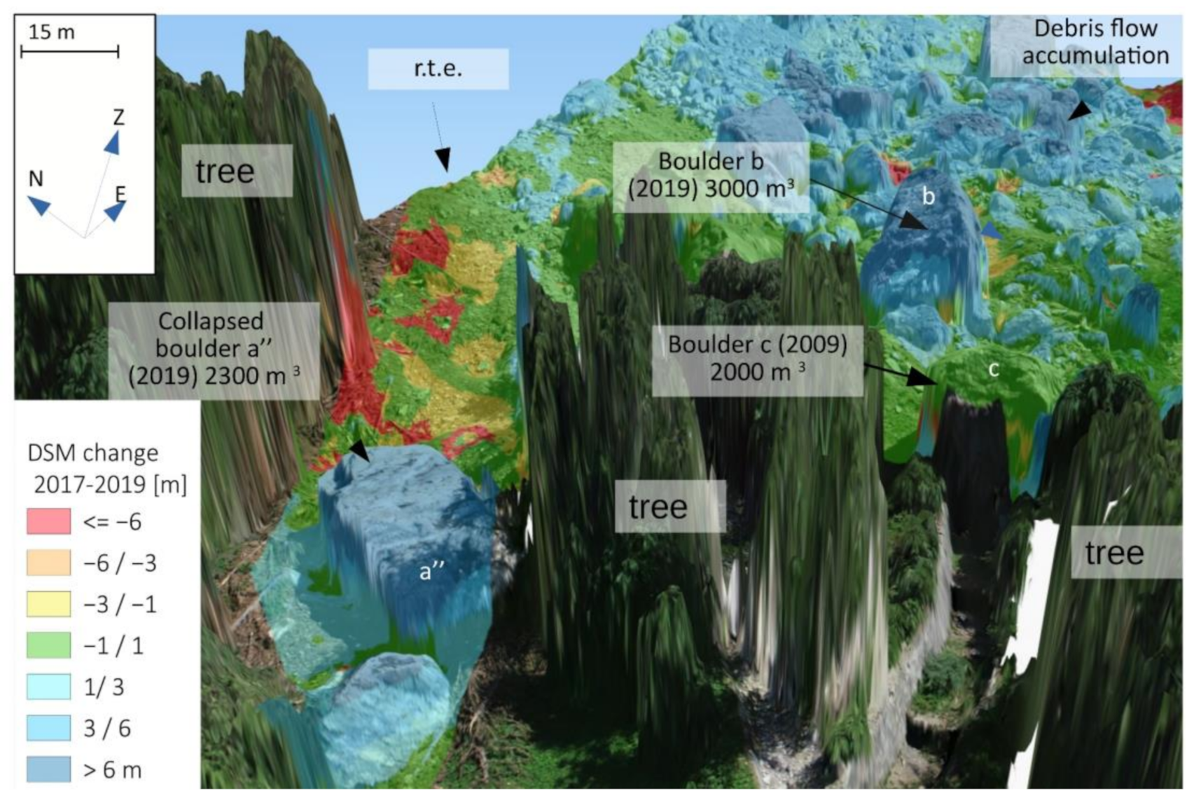
- Deposition sectors (green colors in Figure 13). Most of the debris was deposits in the middle sector of the slope just after the channel (6) at 1400 m a.s.l. Just below this deposit, we can find a dispersed accumulation where most of the boulders stopped (about 211,000 m3) (7); the lower sector of the slope (under 1350 m) is characterized by middle energy deposits blocked by the wall (8) and partly removed by remedial work in July 2019 (8b). Part of the removed material was used to build a new section of the wall (10). On the right side of the accumulation, we can also find the collapsed boulder a” (2000 m3) that stopped about 30 m from the wall (9).
- Low-energy sectors (cyan colors in Figure 13). A small portion of debris flow overpassed the wall for these deposits (11). We calculated the volume for the ‘s’ portion (155 m3) with the method described in Section 3.5 and showed in Figure 8B.
5. Discussion
6. Conclusions
Supplementary Materials
Author Contributions
Funding
Data Availability Statement
Acknowledgments
Conflicts of Interest
References
- Giordan, D.; Adams, M.S.; Aicardi, I.; Alicandro, M.; Allasia, P.; Baldo, M.; De Berardinis, P.; Dominici, D.; Godone, D.; Hobbs, P. The Use of Unmanned Aerial Vehicles (UAVs) for Engineering Geology Applications. Bull. Eng. Geol. Environ. 2020, 79, 3437–3481. [Google Scholar] [CrossRef] [Green Version]
- Giordan, D.; Hayakawa, Y.; Nex, F.; Remondino, F.; Tarolli, P. The Use of Remotely Piloted Aircraft Systems (RPASs) for Natural Hazards Monitoring and Management. Nat. Hazards Earth Syst. Sci. 2018, 18, 1079–1096. [Google Scholar] [CrossRef] [Green Version]
- Daakir, M.; Pierrot-Deseilligny, M.; Bosser, P.; Pichard, F.; Thom, C. UAV Onboard Photogrammetry and GPS Positionning for Earthworks. Int. Arch. Photogramm. Remote Sens. Spat. Inf. Sci. 2015, 40, 293. [Google Scholar] [CrossRef] [Green Version]
- Forlani, G.; Dall’Asta, E.; Diotri, F.; di Cella, U.M.; Roncella, R.; Santise, M. Quality Assessment of DSMs Produced from UAV Flights Georeferenced with On-Board RTK Positioning. Remote Sens. 2018, 10, 311. [Google Scholar] [CrossRef] [Green Version]
- Chiabrando, F.; Lingua, A.; Piras, M. Direct Photogrammetry Using UAV: Tests and First Results. Int. Arch. Photogramm. Remote Sens. Spat. Inf. Sci. 2013, 1, 81–86. [Google Scholar] [CrossRef] [Green Version]
- Zhang, H.; Aldana-Jague, E.; Clapuyt, F.; Wilken, F.; Vanacker, V.; Oost, K.V. Evaluating the Potential of Post-Processing Kinematic (PPK) Georeferencing for UAV-Based Structure-from-Motion (SfM) Photogrammetry and Surface Change Detection. Earth Surf. Dyn. 2019, 7, 807–827. [Google Scholar] [CrossRef] [Green Version]
- Godone, D.; Allasia, P.; Borrelli, L.; Gullà, G. UAV and Structure from Motion Approach to Monitor the Maierato Landslide Evolution. Remote Sens. 2020, 12, 1039. [Google Scholar] [CrossRef] [Green Version]
- Cignetti, M.; Godone, D.; Wrzesniak, A.; Giordan, D. Structure from Motion Multisource Application for Landslide Characterization and Monitoring: The Champlas Du Col Case Study, Sestriere, North-Western Italy. Sensors 2019, 19, 2364. [Google Scholar] [CrossRef] [Green Version]
- Lucieer, A.; de Jong, S.M.; Turner, D. Mapping Landslide Displacements Using Structure from Motion (SfM) and Image Correlation of Multi-Temporal UAV Photography. Prog. Phys. Geogr. 2014, 38, 97–116. [Google Scholar] [CrossRef]
- Rossi, G.; Tanteri, L.; Tofani, V.; Vannocci, P.; Moretti, S.; Casagli, N. Multitemporal UAV Surveys for Landslide Mapping and Characterization. Landslides 2018, 15, 1045–1052. [Google Scholar] [CrossRef] [Green Version]
- Mateos, R.M.; Azañón, J.M.; Roldán, F.J.; Notti, D.; Pérez-Peña, V.; Galve, J.P.; Pérez-García, J.L.; Colomo, C.M.; Gómez-López, J.M.; Montserrat, O.; et al. The Combined Use of PSInSAR and UAV Photogrammetry Techniques for the Analysis of the Kinematics of a Coastal Landslide Affecting an Urban Area (SE Spain). Landslides 2016, 14, 743–754. [Google Scholar] [CrossRef]
- Keilig, K.-P.; Dietrich, A.; Krautblatter, M. Comparison of Multi-Temporal Elevation Models of a Debris-Flow Channel. In Proceedings of the IAEG/AEG Annual Meeting Proceedings, San Francisco, CA, USA, 2018; Springer: Berlin/Heidelberg, Germany, 2019; Volume 1, pp. 275–282. [Google Scholar]
- Liu, C.-C.; Chen, P.-L.; Matsuo, T.; Chen, C.-Y. Rapidly Responding to Landslides and Debris Flow Events Using a Low-Cost Unmanned Aerial Vehicle. J. Appl. Remote Sens. 2015, 9, 096016. [Google Scholar] [CrossRef]
- Stumpf, A.; Malet, J.-P.; Kerle, N.; Niethammer, U.; Rothmund, S. Image-Based Mapping of Surface Fissures for the Investigation of Landslide Dynamics. Geomorphology 2013, 186, 12–27. [Google Scholar] [CrossRef] [Green Version]
- Giordan, D.; Manconi, A.; Tannant, D.D.; Allasia, P. UAV: Low-Cost Remote Sensing for High-Resolution Investigation of Landslides. In Proceedings of the 2015 IEEE International Geoscience and Remote Sensing Symposium (IGARSS), Milan, Italy, 26–31 July 2015; pp. 5344–5347. [Google Scholar]
- Fernández, T.; Pérez, J.L.; Cardenal, J.; Gómez, J.M.; Colomo, C.; Delgado, J. Analysis of Landslide Evolution Affecting Olive Groves Using UAV and Photogrammetric Techniques. Remote Sens. 2016, 8, 837. [Google Scholar] [CrossRef] [Green Version]
- Al-Rawabdeh, A.; He, F.; Moussa, A.; El-Sheimy, N.; Habib, A. Using an Unmanned Aerial Vehicle-Based Digital Imaging System to Derive a 3D Point Cloud for Landslide Scarp Recognition. Remote Sens. 2016, 8, 95. [Google Scholar] [CrossRef] [Green Version]
- Peterman, V. Landslide Activity Monitoring with the Help of Unmanned Aerial Vehicle. Int. Arch. Photogramm. Remote Sens. Spat. Inf. Sci. 2015, 40, 215. [Google Scholar] [CrossRef] [Green Version]
- Hsieh, Y.-C.; Chan, Y.-C.; Hu, J.-C. Digital Elevation Model Differencing and Error Estimation from Multiple Sources: A Case Study from the Meiyuan Shan Landslide in Taiwan. Remote Sens. 2016, 8, 199. [Google Scholar] [CrossRef] [Green Version]
- Jakob, M.; Hungr, O.; Jakob, D.M. Debris-Flow Hazards and Related Phenomena; Springer: Berlin/Heidelberg, Germany, 2005; Volume 739. [Google Scholar]
- Tiranti, D.; Crema, S.; Cavalli, M.; Deangeli, C. An Integrated Study to Evaluate Debris Flow Hazard in Alpine Environment. Front. Earth Sci. 2018, 6, 60. [Google Scholar] [CrossRef]
- Ciurean, R.L.; Hussin, H.; Van Westen, C.J.; Jaboyedoff, M.; Nicolet, P.; Chen, L.; Frigerio, S.; Glade, T. Multi-Scale Debris Flow Vulnerability Assessment and Direct Loss Estimation of Buildings in the Eastern Italian Alps. Nat. Hazards 2017, 85, 929–957. [Google Scholar] [CrossRef] [Green Version]
- Nikolopoulos, E.I.; Borga, M.; Marra, F.; Crema, S.; Marchi, L. Debris Flows in the Eastern Italian Alps: Seasonality and Atmospheric Circulation Patterns. Nat. Hazards Earth Syst. Sci. 2015, 15, 647–656. [Google Scholar] [CrossRef] [Green Version]
- Beniston, M.; Stoffel, M. Rain-on-Snow Events, Floods and Climate Change in the Alps: Events May Increase with Warming up to 4 C and Decrease Thereafter. Sci. Total Environ. 2016, 571, 228–236. [Google Scholar] [CrossRef] [PubMed]
- Gariano, S.L.; Guzzetti, F. Landslides in a Changing Climate. Earth Sci. Rev. 2016, 162, 227–252. [Google Scholar] [CrossRef] [Green Version]
- Turkington, T.; Remaître, A.; Ettema, J.; Hussin, H.; van Westen, C. Assessing Debris Flow Activity in a Changing Climate. Clim. Chang. 2016, 137, 293–305. [Google Scholar] [CrossRef] [Green Version]
- Giorgi, F.; Torma, C.; Coppola, E.; Ban, N.; Schär, C.; Somot, S. Enhanced Summer Convective Rainfall at Alpine High Elevations in Response to Climate Warming. Nat. Geosci. 2016, 9, 584–589. [Google Scholar] [CrossRef]
- Allen, S.K.; Rastner, P.; Arora, M.; Huggel, C.; Stoffel, M. Lake Outburst and Debris Flow Disaster at Kedarnath, June 2013: Hydrometeorological Triggering and Topographic Predisposition. Landslides 2016, 13, 1479–1491. [Google Scholar] [CrossRef]
- Baer, P.; Huggel, C.; McArdell, B.W.; Frank, F. Changing Debris Flow Activity after Sudden Sediment Input: A Case Study from the Swiss Alps. Geol. Today 2017, 33, 216–223. [Google Scholar] [CrossRef]
- Hürlimann, M.; Coviello, V.; Bel, C.; Guo, X.; Berti, M.; Graf, C.; Hübl, J.; Miyata, S.; Smith, J.B.; Yin, H.-Y. Debris-Flow Monitoring and Warning: Review and Examples. Earth Sci. Rev. 2019, 199, 102981. [Google Scholar] [CrossRef]
- Adams, M.S.; Fromm, R.; Lechner, V. High-Resolution Debris Flow Volume Mapping with Unmanned Aerial Systems (UAS) and Photogrammetric Techniques. Int. Arch. Photogramm. Remote Sens. Spat. Inf. Sci. 2016, 41. [Google Scholar] [CrossRef]
- Piana, F.; Fioraso, G.; Irace, A.; Mosca, P.; d’Atri, A.; Barale, L.; Falletti, P.; Monegato, G.; Morelli, M.; Tallone, S. Geology of Piemonte Region (NW Italy, Alps–Apennines Interference Zone). J. Maps 2017, 13, 395–405. [Google Scholar] [CrossRef]
- Tropeano, D.; Luino, F.; Turconi, L. Evento Alluvionale Del 14-15 Ottobre Nell’Italia Nord-Occidentale. Fenomeni Ed Effetti. Geam Torino 2000, 37, 203–216. [Google Scholar]
- Coluccino, M. Fenomeno Franoso del 19.04.2009 Lungo il rio Rich, Versante Sinistro Idrografico Della Val Formazza, a Monte Della Località Ponte (Comune di Formazza, VCO). Rapporto di Valutazione Geologica Preliminare a Seguito del Sopralluogo del 21.04.2009; Provincia del Verbano: Verbania, Italy, 2009. [Google Scholar]
- Boldrini, N. Studio, Caratterizzazione e Valutazione Qualitativa della Pericolosità della Frana di Crollo di Formazza (Località Ponte/Valdo, VB); Milano Bicocca: Milano, Italy, 2010. [Google Scholar]
- Dammeier, F.; Guilhem, A.; Moore, J.R.; Haslinger, F.; Loew, S. Moment Tensor Analysis of Rockslide Seismic Signals. Bull. Seismol. Soc. Am. 2015, 105, 3001–3014. [Google Scholar] [CrossRef]
- Accesso Ai Dati Annali Meteorologici Ed Idrologici Banca Dati Meteorologica. Available online: https://www.arpa.piemonte.it/rischinaturali/accesso-ai-dati/annali_meteoidrologici/annali-meteo-idro/banca-dati-meteorologica.html (accessed on 6 May 2020).
- Notti, D.; Giordan, D.; Caló, F.; Pepe, A.; Zucca, F.; Galve, J. Potential and Limitations of Open Satellite Data for Flood Mapping. Remote Sens. 2018, 10, 1673. [Google Scholar] [CrossRef] [Green Version]
- Giordan, D.; Notti, D.; Villa, A.; Zucca, F.; Calò, F.; Pepe, A.; Dutto, F.; Pari, P.; Baldo, M.; Allasia, P. Low Cost, Multiscale and Multi-Sensor Application for Flooded Area Mapping. Nat. Hazards Earth Syst. Sci. 2018, 18, 1493–1516. [Google Scholar] [CrossRef] [Green Version]
- Gabrlik, P.; la Cour-Harbo, A.; Kalvodova, P.; Zalud, L.; Janata, P. Calibration and Accuracy Assessment in a Direct Georeferencing System for UAS Photogrammetry. Int. J. Remote Sens. 2018, 39, 4931–4959. [Google Scholar] [CrossRef] [Green Version]
- Qgis2threejs Plugin Document—Qgis2threejs Plugin 2.4 Documentation. Available online: https://qgis2threejs.readthedocs.io/en/docs/ (accessed on 22 July 2020).
- ARPA Piemonte. RAPPORTO EVENTO 11/06/2019 Colata Detritica nel Comune di Formazza; ARPA Piemonte: Turin, Italy, 2019; p. 28. Available online: https://www.arpa.piemonte.it/pubblicazioni-2/relazioni-tecniche/analisi-eventi/eventi2019/rapportoformazza. pdf (accessed on 22 July 2020).
- Segoni, S.; Piciullo, L.; Gariano, S.L. A Review of the Recent Literature on Rainfall Thresholds for Landslide Occurrence. Landslides 2018, 15, 1483–1501. [Google Scholar] [CrossRef]
- Guzzetti, F.; Peruccacci, S.; Rossi, M.; Stark, C.P. The Rainfall Intensity–Duration Control of Shallow Landslides and Debris Flows: An Update. Landslides 2008, 5, 3–17. [Google Scholar] [CrossRef]
- Palladino, M.R.; Viero, A.; Turconi, L.; Brunetti, M.T.; Peruccacci, S.; Melillo, M.; Luino, F.; Deganutti, A.M.; Guzzetti, F. Rainfall Thresholds for the Activation of Shallow Landslides in the Italian Alps: The Role of Environmental Conditioning Factors. Geomorphology 2018, 303, 53–67. [Google Scholar] [CrossRef]
- Local Team Frana a Formazza, Case Raggiunte. Il Drone in Volo Sulla Colata—Local Team. Available online: https://www.localteam.it/video/frana-a-formazza-case-raggiunte-il-drone-in-volo-sulla-colata (accessed on 3 July 2020).


| Station Name | Parameters | ID | Distance from the Study Area | Elevation m. a.s.l. |
|---|---|---|---|---|
| Formazza Bruggi | Hourly and daily rainfall | 1 | 3.5 km S | 1226 |
| Formazza Ponte | Snow depth | 2 | 0 | 1300 |
| Larecchio | Snow depth | 3 | 18 km S | 1860 |
| Lago Vannino | Snow depth | 4 | 5 km W | 2177 |
| Formazza | Snow depth | 5 | 9 km NE | 2450 |
| Image Source | Spatial Resolution | Image Acquisition Date | Event Studied | Products Obtained | |
|---|---|---|---|---|---|
| Pre-Event | Post-Event | ||||
| Aerial Photo (Regione Piemonte) | 0.5 m | 2006 | 2010 | 2009 rockslide | Rockslide manual mapping |
| Sentinel-2 | 10 m | 1 June 2019 | 16 June 2019 | 2019 debris flow | NDVIvar, Snow Coverage. |
| RPAS Model | Sector Covered | Flight Date | Photogrammetry Approach | Product Obtained |
|---|---|---|---|---|
| Phantom 4 Pro | S1, S1+S2 | Nov. 2017 (pre-event) | Traditional (GCPs) | DSM, Orthophoto, points cloud |
| Phantom 4 Pro | S1, S1+S2 | July 2018 (pre-event) | Traditional (GCPs) | DSM, Orthophoto, points cloud |
| Phantom 4 Pro | S1, S1+S2 | July 2019 (post-event) | Traditional (GCPs) | DSM, Orthophoto, points cloud |
| Phantom 4 RTK | S2, S1+S2 | July 2019 (post-event) | Traditional (GCPs) Direct (PCPs) & Mixed (GCPs+PCs) | Test of photogrammetry method precision DSM, Orthophoto, points cloud, |
| Camera | Sensor size and memory 1”: 20 M pixel |
| Pixel size = 2.4 μm | |
| Principal distance = 8.8 mm (24 mm FF) | |
| RPAS Model | DJI Phantom 4 RTK |
| Flight | Relative height average on the ground = 100 m |
| Average scale of photos = 1:11300 | |
| Ground Sample Dimension of 1 pixel (GSD) = 2.7 cm | |
| Number of photos: 246 | |
| Ground size of photos 150 m × 100 m | |
| Coverage: along track 80%, across track 70% | |
| Flight time: 11 min mean speed = 7 m/s | |
| Area Measured at ground | 150,000 m2 13 GCPs (50 × 50 cm size marker) |
| Cases | Kind of Adjustment | n. GCP | n. CKP | n. PCP |
|---|---|---|---|---|
| Case 1 | Aerial Triangulation with only 9 GCPs | 9 | 4 | 0 |
| Case 2 | Direct Photogrammetry: i.e., use only PCPs | 0 | 13 | 246 |
| Case 3a | Mixed solution–minimal Case: use only 1 GCP | 1 | 12 | 246 |
| Case 3b | Mixed solution–intermediate case: use 3 GCPs | 3 | 10 | 246 |
| Case 3c | Mixed solution–complete Case use all 13 GCPs | 13 | 0 | 246 |
| RPAS Model | Date | Area Covered km2 | GCPs Count | RMSE (cm) | Image (Pixel) | Pixel Size (m) | ||||
|---|---|---|---|---|---|---|---|---|---|---|
| X (East) | Y (North) | Z (Height) | Total | Orthophoto | DSM | |||||
| Ph4 pro | Nov-17 | 0.188 | 11 | 2.08 | 1.52 | 1.60 | 3.03 | 0.45 | 0.02 | 0.05 |
| Ph4 pro | Jul-18 | 0.218 | 9 | 0.67 | 1.37 | 1.58 | 2.19 | 0.22 | 0.02 | 0.05 |
| Ph4 pro | Jul-19 | 0.264 | 7(2) | 1.51 | 1.40 | 4.60 | 5.04 | 0.62 | 0.05 | 0.05 |
| Residuals Mean and Standard Deviation | Residuals on CKP | Residuals on GCP | ||||
|---|---|---|---|---|---|---|
| n° of CKP | Plan (cm) | h (cm) | n. GCP | Plan (cm) | h (cm) | |
| Case 1 | 4 | 3.1 ± 2.1 | −3.8 ± 1.8 | 9 | 1.3 ± 0.7 | −0.1 ± 3.3 |
| Case 2 | 13 | 3.8 ± 1.6 | 5.9 ± 10.1 | 0 | ||
| Case 3a with 1 GCP M_5 | 12 | 3.7 ± 1.5 | 6.8 ± 10.1 | 1 | ||
| Case 3a with 1 GCP M_13 | 12 | 1.9 ± 1.4 | 2.8 ±10.4 | 1 | ||
| Case 3b | 10 | 1.9 ± 0.8 | 4.7 ± 7.5 | 3 | 2.4 ± 4.9 | 4.9 ± 13.8 |
| Case 3c | 0 | 13 | 1.6 ± 1.0 | 1.6 ± 8.7 | ||
| GCP id | DSMVAR | GCP id | DSMVAR |
|---|---|---|---|
| GCP 106 | 6.71 | GCP 110 | −2.39 |
| GCP 100 | 19.20 | GCP 111 | −11.13 |
| GCP 101 | 9.22 | GCP 103 | 23.14 |
| GCP 102 | −2.27 | GCP 112 | −10.33 |
| GCP 108 | −6.84 | GCP 104 | 0.11 |
| GCP 109 | 30.97 | GCP 105 | 16.21 |
| Sector | ID | Area m2 | DSMVAR (2019–2017) | Volume Change m3 | |
|---|---|---|---|---|---|
| Mean (m) | St. dev. | ||||
| Eroded channel | 1 | 18,799 | −11.00 | 11.80 | −206.8 × 10³ |
| Boulder “a” detach point | 2 | 116 | −10.32 | 6.57 | −1.2 × 10³ |
| Eroded deposits | 3 | 2887 | −5.66 | 7.81 | −16.4 × 10³ |
| Rolling/bounce erosion | 4a | 487 | −1.40 | 0.69 | −0.681 × 10³ |
| Rolling/bounce erosion | 4b | 1172 | −4.21 | 8.77 | −4.94 × 10³ |
| Transit | 5 | 1023 | 0.32 | 0.94 | 0.327 × 10³ |
| Main accumulation | 6 | 28,235 | 7.48 | 4.63 | 211.2 × 10³ |
| Sparse Boulders area | 7 | 18,483 | 2.13 | 3.72 | 39.4 × 10³ |
| Middle energy deposits removed | 8b | 4641 | 1.13 | 2.86 | 5.3 × 10³ |
| Middle energy deposits | 8 | 12,974 | 1.86 | 4.86 | 24.1 × 10³ |
| Boulder “a” stop point | 9 | 438 | 6.42 | 3.36 | 2.81 × 10³ |
| Anthropogenic accumulation | 10 | 4581 | 4.57 | 2.97 | 20.9 × 10³ |
| Lateral debris flow | 11 | 2357 | No data | No data | No data |
| Low-energy debris flow | 12 n | 10,329 | No data | No data | No data |
| Low-energy debris flow | 12 s | 10,587 | The volume was calculated with the interpolation method (0.155 × 10³ m3) | ||
| f (μm) | cx (μm) | cy (μm) | K1 | K2 | K3 | K4 | ||
|---|---|---|---|---|---|---|---|---|
| Case 3-c PC + 13 GCP | m= | 8757.480 | −8.277 | 16.434 | −0.653 | 0.295 | −0.128 | 0.029 |
| σ= | 0.113 | 0.046 | 0.038 | 5.04 × 10⁻⁵ | 1.65 × 10⁻⁴ | 2.01 × 10⁻⁴ | 8.33 × 10⁻⁵ | |
| Case 3-a PC + 1 GCP | m= | 8742.528 | −8.532 | 16.309 | −0.651 | 0.293 | −0.127 | 0.029 |
| σ= | 0.312 | 0.046 | 0.038 | 6.82 × 10⁻⁵ | 1.67 × 10⁻⁴ | 1.99 × 10⁻⁴ | 8.16 × 10⁻⁵ |
Publisher’s Note: MDPI stays neutral with regard to jurisdictional claims in published maps and institutional affiliations. |
© 2021 by the authors. Licensee MDPI, Basel, Switzerland. This article is an open access article distributed under the terms and conditions of the Creative Commons Attribution (CC BY) license (https://creativecommons.org/licenses/by/4.0/).
Share and Cite
Notti, D.; Giordan, D.; Cina, A.; Manzino, A.; Maschio, P.; Bendea, I.H. Debris Flow and Rockslide Analysis with Advanced Photogrammetry Techniques Based on High-Resolution RPAS Data. Ponte Formazza Case Study (NW Alps). Remote Sens. 2021, 13, 1797. https://doi.org/10.3390/rs13091797
Notti D, Giordan D, Cina A, Manzino A, Maschio P, Bendea IH. Debris Flow and Rockslide Analysis with Advanced Photogrammetry Techniques Based on High-Resolution RPAS Data. Ponte Formazza Case Study (NW Alps). Remote Sensing. 2021; 13(9):1797. https://doi.org/10.3390/rs13091797
Chicago/Turabian StyleNotti, Davide, Daniele Giordan, Alberto Cina, Ambrogio Manzino, Paolo Maschio, and Iosif Horea Bendea. 2021. "Debris Flow and Rockslide Analysis with Advanced Photogrammetry Techniques Based on High-Resolution RPAS Data. Ponte Formazza Case Study (NW Alps)" Remote Sensing 13, no. 9: 1797. https://doi.org/10.3390/rs13091797