Hydrodynamic Modelling for a Transportation System of Two Unmanned Underwater Vehicles: Semi-Empirical, Numerical and Experimental Analyses

Abstract

Underwater transportation is an essential approach for scientific exploration, maritime construction and military operations. Determining the hydrodynamic coefficients for a complex underwater transportation system comprising multiple vehicles is challenging. Here, the suitability of a quick and less costly semi-empirical approach to obtain the hydrodynamic coefficients for a complex transportation system comprising two Unmanned Underwater Vehicles (UUVs) is investigated, where the interaction effects between UUVs are assumed to be negligible. The drag results were verified by Computational Fluid Dynamics (CFD) analysis at the steady state. The semi-empirical results agree with CFD in heave and sway; however, they were overpredicted in surge due to ignoring the wake effects. Furthermore, experiments were performed for the validation of the time-domain motion simulations with semi-empirical and CFD results. The simulations which were performed with the CFD drags were close to the experiments. The semi-empirical approach could be relied on once a correction parameter is included to account for the interactive effect between multiple UUVs. Overall, this work makes a contribution by deriving a semi-empirical approach for the dynamic and controlling system of dual UUVs, with CFD and experiments applied to ascertain its accuracy and potential improvement.

1. Introduction

Underwater transportation is an important requirement for the scientific, commercial and military sectors as it can place an underwater structure at a precise location [1,2,3]. Unmanned Underwater Vehicles (UUVs) can be used in different systems to undertake underwater transportation based on the connection between the vehicles and the payload, i.e., Rigid Connection Transportation System (RCTS) and Flexible Connection Transportation System (FCTS). In RCTS, UUVs are connected to the payload via solid links as used in [4,5,6,7]. The whole system is considered to be a single body. Alternatively, in FCTS the vehicles are connected to the payload via flexible links, as adopted in [8,9,10,11,12], where there is a relative motion between the vehicles and the payload. In this paper, hydrodynamic modelling is studied for an RCTS system operating underwater.

The development of the dynamic model for an underwater transportation system is vital to design stable, robust, high-accuracy and low-power-consumption control systems. The dynamic model consists of inertia, hydrostatic and hydrodynamic terms. The inertia and hydrostatic parameters can be directly measured with accuracy as they mainly depend on the physical system. The hydrodynamic parameters describe the opposition to the motion of the system due to the medium in which it is moving. Obtaining an accurately tuned dynamic model for an ROV and designing an appropriate control system are challenging due to the uncertainties in the hydrodynamic parameters [13,14]. The difficulty increases for complex systems comprising multiple vehicles. It is important that the hydrodynamic parameters for an underwater vehicle or an underwater system are determined accurately, which can be performed experimentally, numerically or semi-empirically.

A wide range of different experimental methods has been used to determine the hydrodynamic parameters of UUVs. For example, a planar motion mechanism (PMM) can be used to forcibly oscillate the vehicle whilst being towed through water in a towing tank; in [15], PMM was employed to work out the hydrodynamic coefficient for an open-frame ROV called LAURS. An alternative approach, the free decay test, can also be used to work out the hydrodynamic coefficients [16,17]. This technique was first proposed by Morisons [18] on ROV Hylas for determining the hydrodynamic coefficients in heave. In his procedure, the ROV was suspended in water and then released with the oscillations decaying over time. The hydrodynamic coefficients were calculated from the recorded location data history. Currently, the System Identification (SI) technique is widely used to determine the model parameters of UUVs from free water trials [19,20,21]. Here, the data of onboard sensors and the control signals of thrusters are used to identify the parameters. This technique is relatively cheaper than using a PMM and repeatability is high [15]. However, the accuracy of the parameters is affected due to sensor noise, which is caused by the magnetic field of the thruster motors, and due to difficulties in determining the thrusters’ actuation forces/moments exactly [15].

Mesh-based CFD methods, e.g., Finite Volume Method (FVM), can account well for complex structures, such as UUVs. FVM allows for the precise representation of a complex geometry inside a computational domain, in which a 3D geometry may be expressed as a closed surface that is in contact with numerous computational cells, which fully accounts for its structural complexity and boundary effect. The fluid fields outside the geometry and inside the computational domain can be obtained through solving fully nonlinear Navier–Stokes equations [22]. The accuracy of CFD has been reported to be very good for hydrodynamic problems where a solid body interacts with fluid flows [23,24,25,26,27] with viscous and turbulent flows being well modelled [28,29,30,31,32]; particular CFD studies on UUVs can be seen in [33,34,35,36,37,38,39].

Although the CFD and experimental methods can provide accurate results, they are generally time-consuming and expensive. This is a problem especially for multi-vehicular transportation systems due to their complexity and reconfigurability to many different arrangements. Therefore, a semi-empirical approach is preferred for determining hydrodynamic parameters in many studies [40,41,42,43,44]. Due to its rapidity and low cost, the estimated parameters using the semi-empirical method help in the optimal design of an underwater vehicle and to predict its behaviour [45]. Moreover, the parameters could be used for the plant/controller optimisation for increased performance of an underwater vehicle before it is fabricated and tested [46].

The semi-empirical approach of estimating the hydrodynamic coefficients for an underwater vehicle is mainly based on Morison’s equation [47], which divides the parameters into non-viscous added mass and viscous damping terms. The added mass part is derived based on the potential flow theory and the drag part is obtained from the experimental analysis. Hence, the term “semi-empirical” stems from the added mass term coming from a fluid dynamics model, whereas the viscous drag term is from an empirical coefficient.

There are high uncertainties associated with the assumptions which are made in the semi-empirical method of calculating hydrodynamic coefficients. For instance, when Det Norske Veritas (DNV) standards [48] are used to calculate the added mass of an ROV, as accomplished in [40], it was assumed that the vehicle is a rectangular prism where two of the three sides are equal or the difference between two of the three sides is not more than ±10%. Moreover, the ROV was initially assumed to be a solid prism; therefore, the results needed adjusting to account for the gaps. Therefore, the results of the semi-empirical approach need to be verified and validated and necessary coefficients must be added to make the approach’s application feasible.

Hydrodynamic models have been developed for a single UUV based on a semi-empirical approach. Prestero [41] developed a semi-empirical hydrodynamic model for a torpedo-shaped Autonomous Underwater Vehicle (AUV). The empirical formula was used to work out the drag term in the axial direction, whereas strip theory was used for the drag terms in other direction separately for the cylindrical hull and fins. The coefficients were used from the empirical data. The roll drag was estimated by considering only the fins, as the major portion of rolling resistance comes from fins. For the axial added mass term, the vehicle hull was approximated by an ellipsoid for which the major axis is half the vehicle length and the minor axis is half the vehicle diameter. The added mass terms in other directions were worked out using the strip theory separately for the cylindrical and cruciform hull cross-sections. The rolling added mass was calculated only for the fins as the smooth hull sections only generate a small added mass in roll which was neglected. The empirical formulas were used to work out the body and fin lift coefficients in all directions. Humphreys [44] worked out the added mass terms in detail for each part of a torpedo-shaped AUV using the semi-empirical approach. In [43], the lift, drag and pitching moment coefficients were calculated for a bare hull AUV using the semi-empirical equations which were derived in the literature, and CFD analysis was carried out to verify them. In [42], analytical and semi-empirical (ASE) methods were used to approximate the hydrodynamic parameters for AUV. Eidsvik [40] calculated the hydrodynamic parameters for a box-shaped Remotely Operated Vehicle (ROV) using the DNV-standard [48], which is based on the Applied Fluid Dynamics book by Blevins [49]. In his approach, the ROV was assumed to be a solid prism where two to three sides are equal. This assumption could be true for some specific ROVs such as SF-30k, AC-ROV 100, Seabotics LBV600-6 and Videoray PRO-4, where the height and width are approximately the same. Appropriate scaling coefficient was included to account for the penetrating flow through the ROV. The translational added mass terms were calculated using the potential flow data. However, the 3D data for the rotational added mass terms could not be found. Therefore, they were approximated by the 2D data and strip theory. The translational drag terms were calculated using the empirical. Again, the 3D data for the rotational drag parameters were not available. Therefore, they were approximated for small angles where rotational motion can be transformed to translational motion.

The calculation of hydrodynamic parameters for complex-shaped underwater vehicles or the underwater systems which consist of multiple UUVs is lacking in the literature. Therefore, hydrodynamic models are required to be developed for such systems. Moreover, the semi-empirical approach needs to be improved to reduce hydrodynamic uncertainties. The contribution of this work is twofold: (1) an effective semi-empirical approach is introduced to estimate the hydrodynamic coefficients for a system of multiple UUVs; (2) the method is verified against CFD results and validated with experimental measurements.

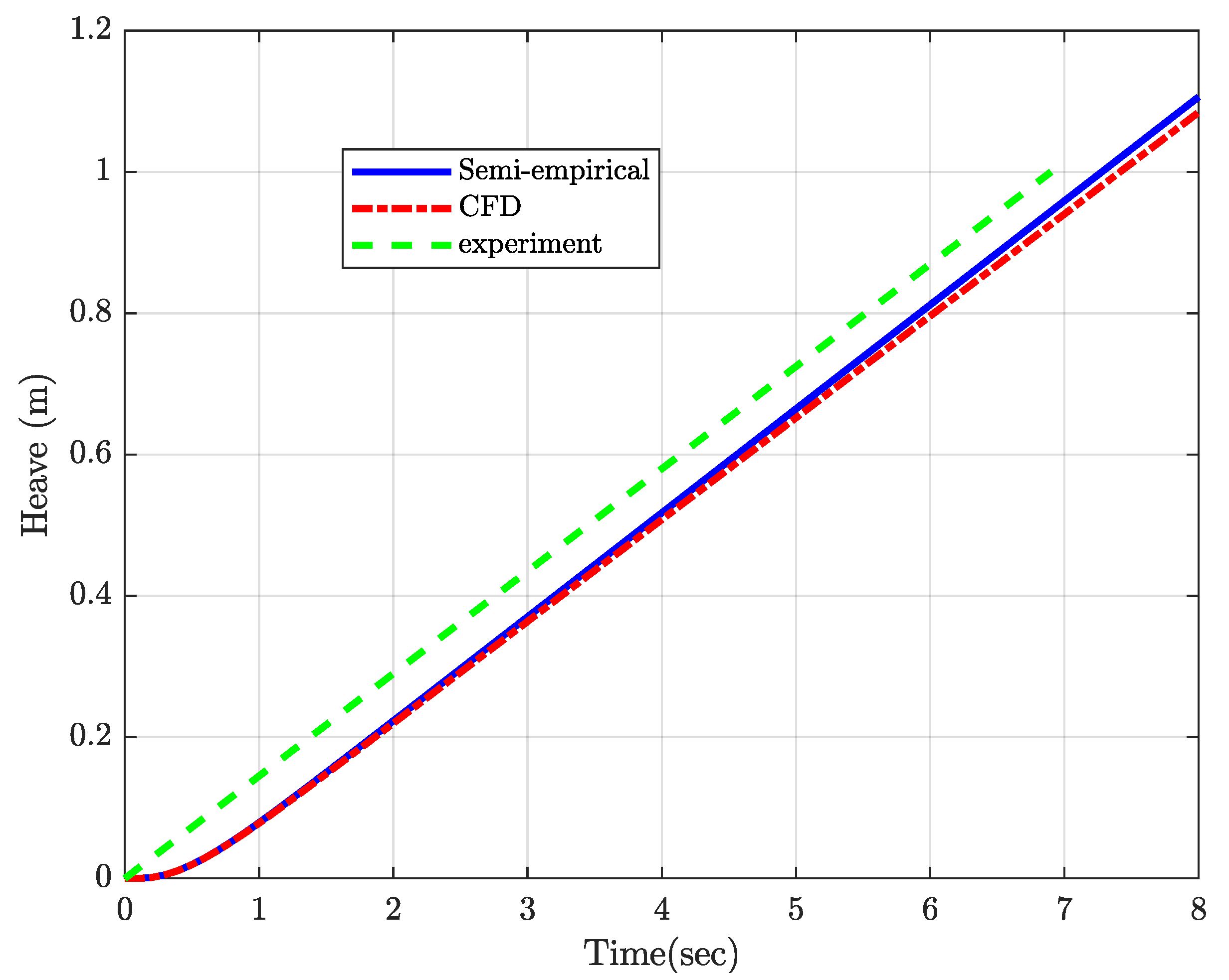
In this paper, the hydrodynamic parameters were not calculated in the experiments. Instead, the system was run in the towing tank and its motion response was recorded in the time domain. On the other hand, the dynamic model was developed for the system with the calculated hydrodynamic parameters from, respectively, the semi-empirical approach and CFD. The time-domain motion simulations were performed on the dynamic model. The motion response of the simulations was compared to the experiments for validation. A similar approach was used by Singh [50] for an underwater glider in which the hydrodynamic parameters were calculated using CFD analysis. These coefficients were used in the motion equations proposed by Leonard and Graver [51] in the vertical plane to obtain a simulation model. Subsequently, the motion response in simulations was compared to the experiments for validation.

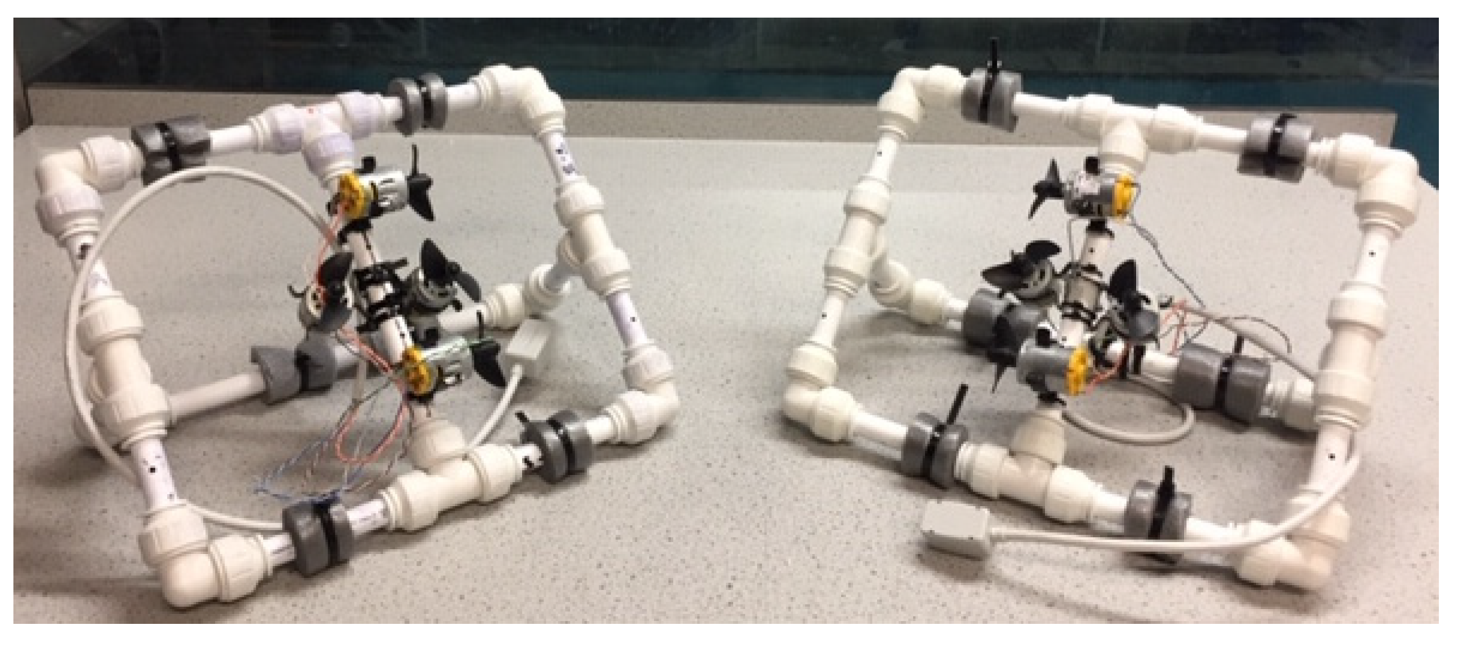
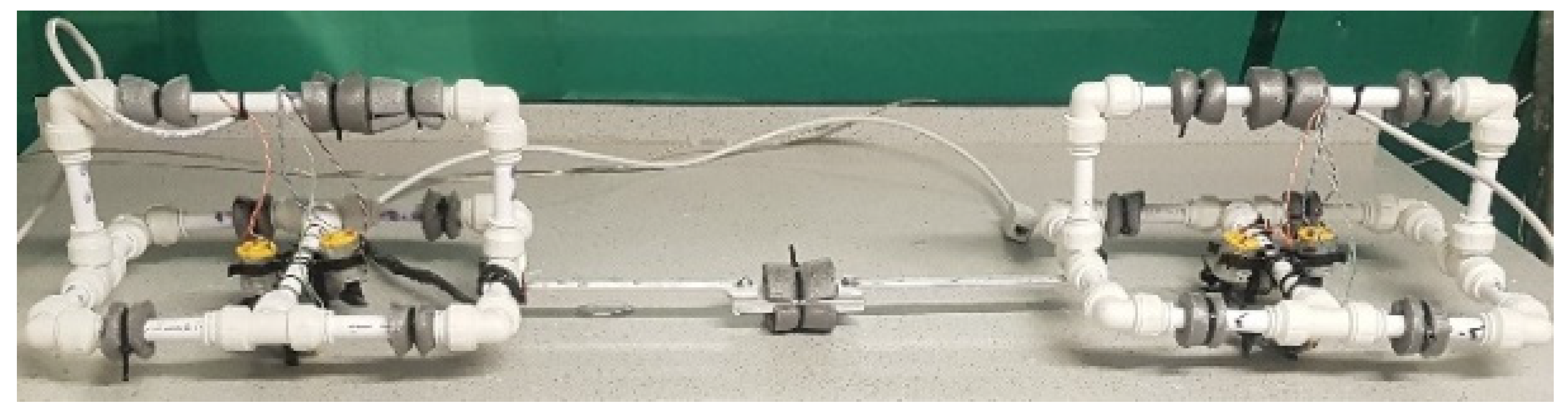
The rest of the paper is arranged as follows. Section 2 describes the fabrication of the rigid connection transportation system (RCTS), which was tested in the towing tank and velocities were measured. This system, comprising two UUVs, represents the case study analysed in this work. In Section 3, the hydrodynamic parameters are calculated using the semi-empirical approach and the drag forces are verified with CFD analysis. A dynamic model is also developed to run time-domain motion simulations. In Section 4, the drag forces, which are obtained by semi-empirical and CFD methods, are compared and the difference is discussed to analyse the potential deficiency of the semi-empirical approach. The time-domain motion simulations are carried out with the coefficients computed with both methods, which are compared to the experiments for validation. Finally, concluding remarks are given in Section 5.

2. Experiment

The hydrodynamic modelling is performed on an available system that can be tested in the towing tank for validation.

2.1. Fabrication

For the dual UUVs transportation system, which is rigidly connected to the payload, two identical modified Seaperch UUVs [52,53] were fabricated using PVC pipes which were connected through elbows and T joints, as shown in Figure 1. The sizes of pipe, elbow and T-joint are shown in

Table 1. Size of pipe, elbow and T-joint of Seaperch UUV.

	Size
Pipe	Diameter = 1.65 ± 0.1 cm
Elbow	$L_1\times L_2\times D=3.5\pm 0.1\mathrm{cm}\times 3.5\pm 0.1\mathrm{cm}\times 3\pm 0.1\mathrm{cm}$
T-joint	$L_1\times L_2\times L_3\times D=2.4\pm 0.1\mathrm{cm}\times 2.4\pm 0.1\mathrm{cm}\times 2.4\pm 0.1\mathrm{cm}\times 3\pm 0.1\mathrm{cm}$

.

This design of Seaperch was selected as it is highly stable with a COG well below its COB. Four thrusters were attached to each Seaperch: two to move the vehicle in the vertical direction and two to move the UUV in the axial direction. Each vehicle is underactuated as no thrusters are applied in the transverse direction, so that only surge, heave, pitch and yaw can be controlled.

After the fabrication, the mass and volume of each UUV were measured to determine the weight and buoyancy. The COG of each vehicle was also measured, whilst the COB of the vehicle was calculated using the COB and volume of each part of the vehicle.

In practice, the underwater vehicles are made slightly positively buoyant so that they rise to the sea surface in case of an emergency [54]. However, for research studies, especially for designing the control systems, the test models are made to be neutrally buoyant to ease analysis [40,55,56,57,58]. Therefore, each Seaperch UUV was made neutrally buoyant, and after attaching the manipulators and payload to the UUVs, the whole system was made neutrally buoyant by attaching small patches of buoyancy sheet. The power cables were made neutrally buoyant to nullify their impact on the hydrostatic parameters. After fabrication and connections, the whole system is shown in Figure 2.

A MATLAB program was developed to provide input to the thrusters of the system using the Arduino hardware. An initial estimate of the dynamic stability of the system was obtained from the Routh Hurwitz criteria [59]. However, after the fabrication of the system, several initial tests were performed to ensure the dynamic stability of the system. The parameters of the fabricated RCTS are shown in

Table 2. RCTS parameters.

Parameters	Values
$\mathrm{Mass}\mathrm{of}\mathrm{Seaperch}\mathrm{UUV}\left(m_{ROV}\right)$	0.8 kg ± 0.02 kg
$\mathrm{Mass}\mathrm{of}\mathrm{RCTS}\left(m\right)$	1.97 ± 0.05 kg
Centre of Buoyancy from Keel (COB)	(1.8 ± 0.1 cm, 0 cm, 0 cm)
Centre of Gravity from Keel (COG)	(2.5 ± 0.1 cm, 0 cm, 0 cm)

, including instrument precision.

2.2. Velocity Measurement

In tests conducted in the UCL towing tank, the system was given a constant thrust input via the Arduino hardware and the time taken to achieve the marked distances on the towing tank glass boundary was measured. The acceleration stage was assumed to last a short time from simulations and was thus neglected. The velocities, which were measured in surge and heave, are shown in

Table 3. Measured velocities.

Velocity	Value (m/sec)
Surge	0.167 ± 0.0058
Heave	0.144 ± 0.016

. An uncertainty analysis was undertaken to quantify the systematic and random errors, with the uncertainty being driven low by repeating the tests multiple times.

3. Hydrodynamic Modelling

In this section, the hydrodynamic forces are calculated for the fabricated RCTS using the semi-empirical approach, with each piece of the Seaperch UUV, manipulator and payload being analysed separately and then summed together. Additionally, in this section, a CFD model was built and used to obtain the drag forces.

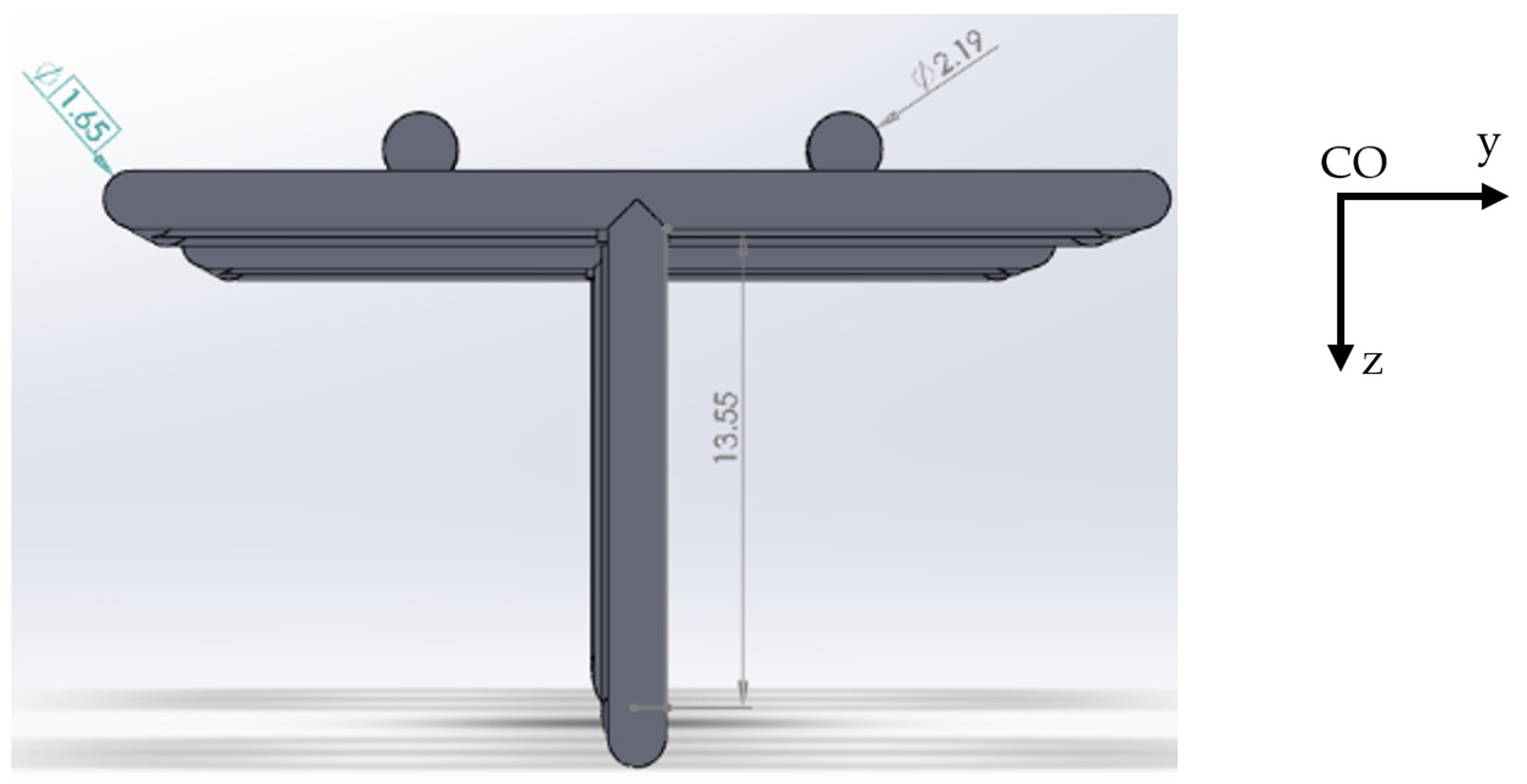
3.1. Geometry

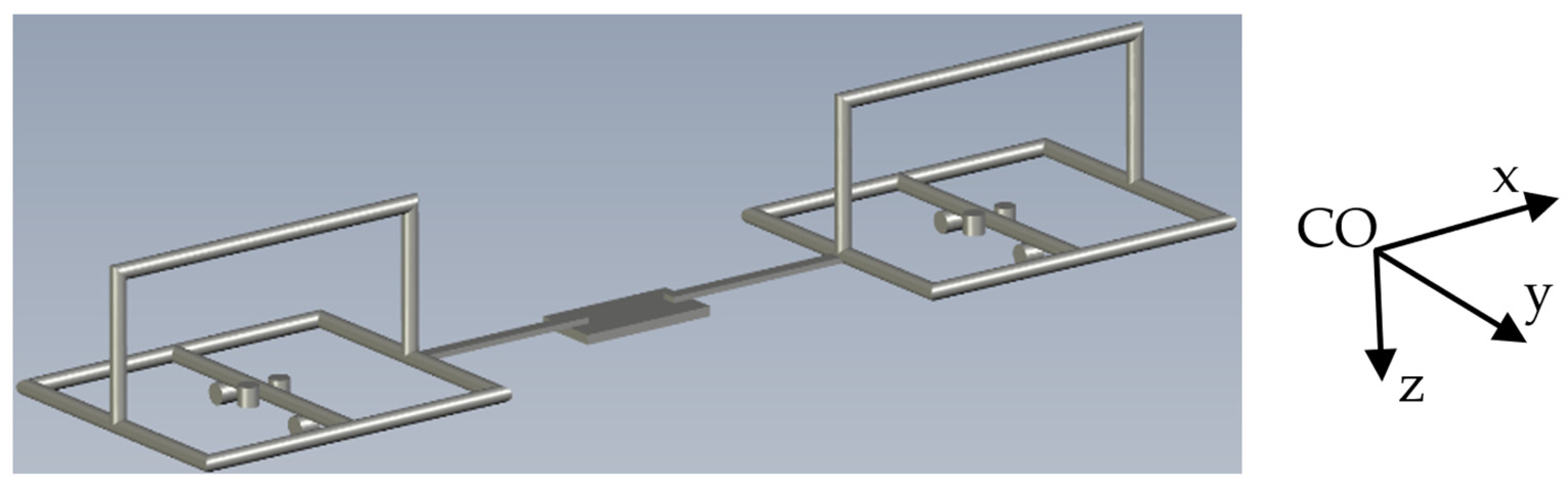
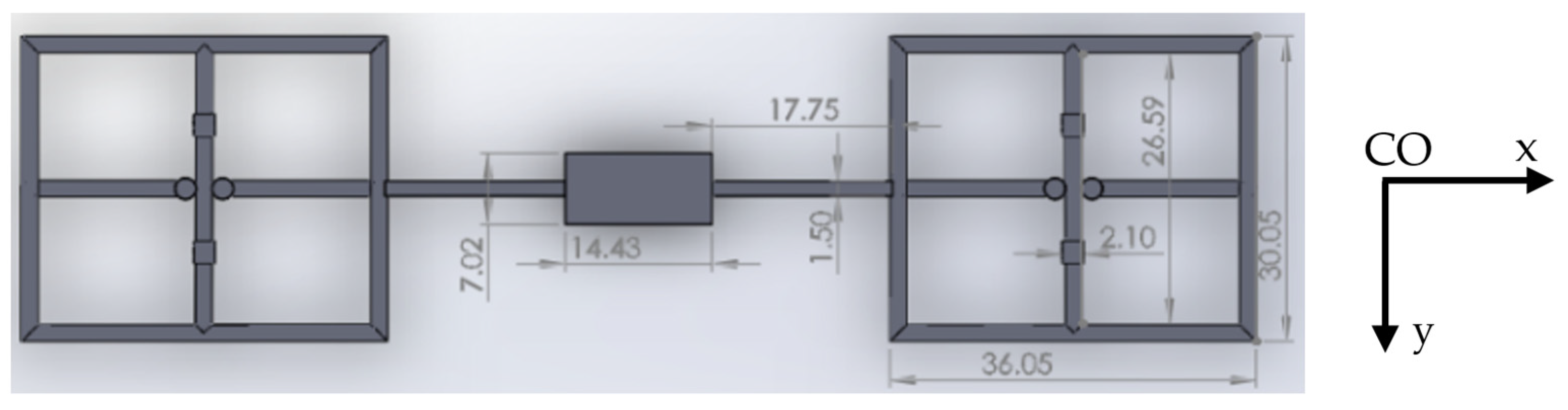
A 3D model of the system was produced in the SolidWorks software [60], as shown in Figure 3. The plan, profile and front views are shown in Figure 4, Figure 5 and Figure 6, respectively.

3.2. Assumptions

The following assumptions were made when calculating the hydrodynamic parameters for the studied system using the semi-empirical and CFD methods:

• The system is a rigid body, i.e., there is no relative motion between the mass particles of the system. This is generally true as the parts on the system were not found to bend during testing.
• The system’s mass and its distribution do not change during the motion. This is a valid assumption and ensured during testing.
• The system is operating below base wave depth, i.e., the depth at which the sea wave effects are negligible. The baseline depth is equal to $\lambda /2$ where $\lambda$ is equal to the wavelength [61]. This was ensured in the experiments.
• The system only has translational motion, i.e., in surge, sway and heave. This was ensured during experiments as only the respective thrusters were used for motion in each direction and no disturbances were included.
• The vehicle does not experience a memory effect, i.e., the vehicle does not pass through its own wake.
• The vehicle does not experience the ocean current. The calm water in the towing tank would have negligible water currents.
• Interaction with the seabed or other underwater bodies is neglected. This was ensured during the experiments.
• The flow interaction amongst the parts of the system is ignored in the semi-empirical approach. This is something of concern and could be the main reason to cause an error. This effect is accounted for in CFD.
• The blades of the thrusters are ignored. They are small in size; therefore, their effect on the overall hydrodynamic results is small.
• The elbows and T-joints are considered to have pipes of the same inner and outer diameters as of the other pipes, and the length is the same as of the respective elbow or T-joint. This would have a small impact as the extended portion of elbows and T-joint is only 6.5 mm.
• The impact of buoyancy sheet patches on the hydrodynamic parameters is also ignored.

Although the system is underactuated and cannot move in pure sway, the added mass and drag forces were calculated in all three translational directions, i.e., surge, sway and heave. The velocity in sway is assumed to be the same as in surge.

3.3. Semi-Empirical Approach

The semi-empirical methods which are mostly applied in the literature to calculate the hydrodynamic parameters for a single UUV consider the whole vehicle, either a cylinder with fins or a solid prism. However, they are only true for specific types and shapes of UUVs. For the complex shaped UUV or a system of multiple UUVs, there is a lack of research in the literature to work out the hydrodynamic parameters. Therefore, in this study, a different approach of estimating the hydrodynamic parameters for an underwater vehicle is proposed, in which the system is cut down to simple individual parts. The parameters are calculated for each part and combined to obtain the net effect.

The hydrodynamic parameters were calculated for one Seaperch UUV and one manipulator plate, which were then doubled to obtain the effect of two Seaperch UUVs and two manipulators. The payload plate was evaluated separately. For the Seaperch UUV, the hydrodynamic parameters were evaluated separately for each pipe and thruster motor. They were then summed to obtain the net effect in each direction. The system parts are shown in

Table 4. Quantity of each part in the combined system.

Serial Number	Parts	Quantity
1.	30.05 m pipe	04
2.	26.59 cm pipe	02
3.	36.05 cm pipe	06
4.	13.55 cm pipe	04
5.	Axial thruster motors	04
6.	Vertical thruster motors	04
7.	Manipulator plate	02
8.	Payload plate	01

.

3.3.1. Added Mass

The added mass is the inertia added to the vehicle as it displaces the surrounding water during acceleration or deceleration. The calculation of added mass does not take into account the viscous effects. The added mass part of Morison’s equation for a solid body is given as [47]:

$$A_i=\rho C_a{V}_R,$$

(1)

where $A_i$ is the added mass term due to acceleration $i$ or, in other words, the derivative of the added mass w.r.t acceleration $i$. For instance, the added mass terms in surge, sway and heave are $X_{\dot{u}}$, $Y_{\dot{v}}$ and $Z_{\dot{w}}$, respectively. $\rho$ is the density of water (in this case, freshwater), $C_a$ is the added mass coefficient and $V_R$ is the reference volume.

The added mass terms were calculated separately for each pipe and thruster motor of the Seaperch UUV and for the manipulator and payload plates using the data which are based on the DNV standards [48]. The detailed calculations are shown in Appendix A. After calculations, the added mass terms for each part of the system are shown in

Table 5. Added mass terms calculated for each part.

Serial Number	Parts	Surge (kg)	Sway (kg)	Heave (kg)
1.	30.05 m pipe	0.064	0	0.064
2.	26.59 m pipe	0.057	0	0.057
3.	36.05 cm pipe	0	0.077	0.077
4.	13.55 cm pipe	0.027	0.027	0.0025
5.	Axial thruster motors	0.005	0.004	0.004
6.	Vertical thruster motors	0.004	0.004	0.005
7.	Manipulator plate	0.002	0.002	0.01
8.	Payload plate	0.0022	0.0022	0.15

. They were summed together to obtain the total added mass terms in each surge, sway and heave, as shown in

Table 6. Total added mass terms.

Serial Number	Parts	Quantity	Surge (kg)	Sway (kg)	Heave (kg)
1.	30.05 m pipe	04	0.256	0	0.256
2.	26.59 m pipe	02	0.114	0	0.114
3.	36.05 cm pipe	06	0	0.462	0.462
4.	13.55 cm pipe	04	0.11	0.11	0.01
5.	Axial thruster motors	04	0.02	0.016	0.016
6.	Vertical thruster motors	04	0.016	0.016	0.02
7.	Manipulator plate	02	0.004	0.004	0.02
8.	Payload plate	01	0.0022	0.0022	0.15
	Total		0.52	0.61	1.05

. The impact of added mass on the overall motion response would be less significant due to the short acceleration duration.

The added mass terms are added to the total mass of the system to obtain the net inertia terms, which are then multiplied by the accelerations to obtain the inertial forces.

3.3.2. Drag

The resistance to the motion of the vehicle due to the viscosity of water is called drag. The drag part of Morison’s equation for a solid body is given as [47]:

$$B_i=\frac{\rho }{2}{C}_{D/f}{A}_{c/s},$$

(2)

where $B_i$ is the drag term due to velocity $i$. For instance, the drag terms in surge, sway and heave are $X_{u\left|u\right|}$, $Y_{v\left|v\right|}$ and $Z_{w\left|w\right|}$, respectively. $C_{D/f}$ is the drag coefficient where $D$ or $f$ depends on the form or frictional drag, which further depends on the shape of the part in front of the flow and the flow velocity. The drag coefficients were also calculated from the data based on DNV standards given in [48]. $A_{c/s}$ is the cross-sectional or surface area depending on the form or frictional drag.

Initially, it is important to know whether the flow over a body predominantly exerts form or frictional drag.

Similar to the added mass, the drag terms were calculated separately for each part of the Seaperch UUVs, manipulators and payload. Initially, it was worked by Reynold’s number (Re) whether the flow over a part body predominantly exerts form or frictional drag.

The detailed calculations are shown in Appendix B. The total drag terms for the system in surge, sway and heave are shown in

Table 7. Total drag terms.

Serial Number	Parts	Surge (kg/m)	Sway (kg/m)	Heave (kg/m)
1.	30.05 cm pipe	7.2	0.612	7.2
2.	26.59 cm pipe	3.16	0.28	3.16
3.	36.05 cm pipe	1.02	13.38	13.38
4.	13.55 cm pipe	2.96	2.96	0.445
5.	Axial thruster motors	0.628	0.48	0.48
6.	Vertical thruster motors	0.48	0.48	0.628
7.	Manipulator plate	0.011	0.039	5.7
8.	Payload plate	0.017	0.031	5.93
	Total	15.5	18.26	36.92

.

The drag forces in surge, sway and heave were obtained by multiplying the drag terms by the square of the velocities in each direction.

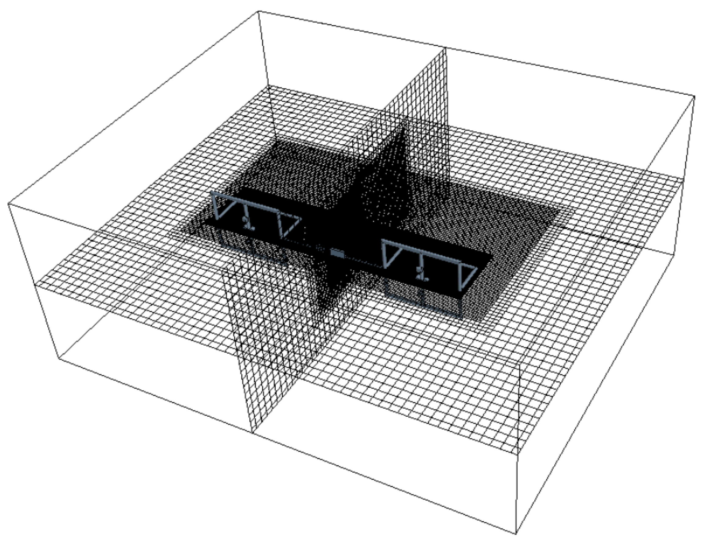
3.4. CFD Analysis

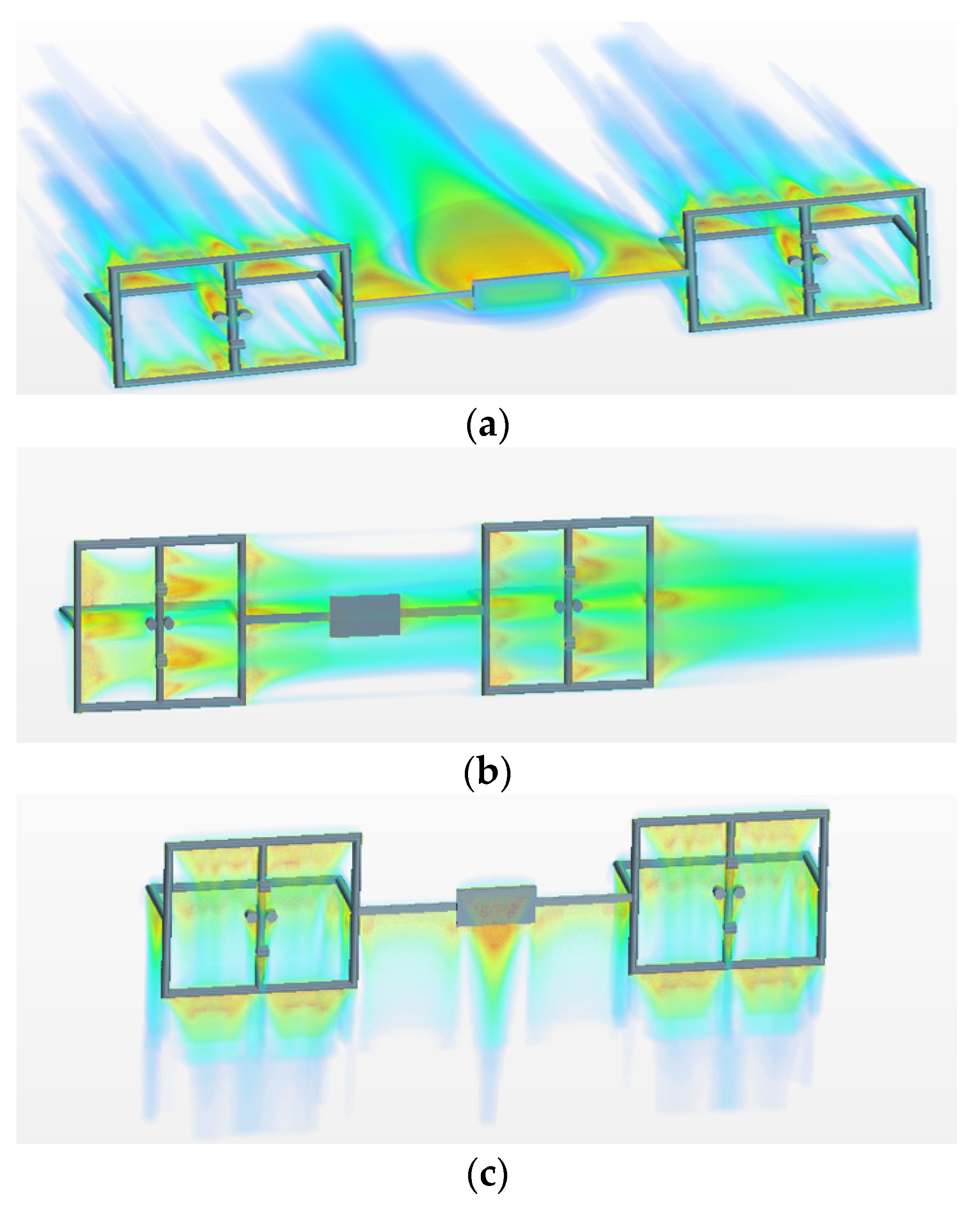
The computational domain was built for the studied transportation system introduced in Section 2, using the STAR-CCM+ CFD software [62]. A three-dimensional cuboid computational domain was established, and the transportation system is fixed in the middle of the domain, as shown in Figure 7. The domain size is sufficiently large to avoid the system feeling any boundaries, in line with the experiments. The boundary conditions consist of a velocity inlet and a pressure outlet to propagate a constant flow against the device. The other four boundaries were defined as zero-gradient to model far fields. The domain is filled with water, and the water was defined as flowing with a constant velocity (U_water) against the system. Thus, a relative velocity exists between the system and water, where U_water indicates the advancing speed of the system in calm water (U_water = U), which is known in surge, sway and heave. This approach is similar to previous work studying the hydrodynamic performance of objects in water [63,64]. The direction of the water flow is set according to different motions of the system, as shown in Figure 8, in which the corresponding velocity fields at steady state are presented.

The solution of the fluid domain was obtained by solving the Reynolds-averaged Navier–Stokes (RANS) equations for an incompressible Newtonian fluid:

$$\nabla \cdot \overline{v}=0$$

(3)

$$\frac{\partial \left(\rho \overline{v}\right)}{\partial t}+\nabla \cdot \left(\rho \overline{vv}\right)=-\nabla \overline{p}+\nabla \cdot \left(\overline{\tau }-\rho \overline{v^{\prime }{v}^{\prime }}\right)+\rho g$$

(4)

where $\overline{v}$ is the time-averaged velocity, $v^{\prime }$ is the velocity fluctuation, ρ is the fluid density, $\overline{p}$ denotes the time-averaged pressure, $\overline{\tau }$ = µ [∇v+ (∇v)^T] is the viscous stress term, µ is the dynamic viscosity and g is gravitational acceleration set at 9.81 m/s². The density of the water was set at 1000 kg/m³ and the dynamic viscosity was 8.90 × 10⁻⁴ N·s/m². Since the RANS equations have been adopted to account for the turbulent effects, a turbulence model needs to be applied; here, the Shear Stress Transport (SST) k − ω model was adopted to close the equations.

The drag force is the steady-state force from fluid on the transportation system against the motion. This can be calculated as the integration of pressure and viscous forces on the system’s surface depending on the direction of motion.

The mesh was refined around the device and for the nearby flow field. Following the ITTC guideline [65], the mesh was globally scaled by a factor of $\sqrt{2}$, which resulted in three mesh sets of, respectively, 1.56, 2.2 and 3.1 million cells. The corresponding drag forces in heave are 0.75, 0.80 and 0.80 N, which means the drag achieved convergence at 2.2 million cells, and further increasing the cells to 3.1 million could not alter the results. Therefore, the mesh set with 2.2 million cells was applied for further studies to save computational costs. The time step size was set based on the Courant number equalling to one. The applied CFD is a standard method and the numerical setup follows mature guidelines of the field [65], which has been extensively validated to be highly accurate, while this specific CFD model will be further validated by an experimental model introduced later.

3.5. Dynamic Modelling

The dynamic model is developed for the transportation system to run the time-domain motion simulations. Fossen’s approach [66] is used in the development of the dynamic model in which the position and orientation of the system are defined in the earth-fixed frame (EFF), whereas velocities, forces and moments are defined in the body-fixed frame (BFF). Though the power cables were made neutrally buoyant, their inertia would have an impact on the overall inertia of the system. However, the inertia of the power cables was ignored in the system’s dynamic model due to the difficulty of taking their effect on the centre of origin of the system (CO). Moreover, assumptions 1 to 7 in Section 3.2 were also made in the development of the dynamic model for the studied transportation system.

The kinematics provides the change in the position and orientation of the system, which is written in the vectorial form as:

$$\dot{\mathit{\eta }}=\mathit{J}\mathit{v},$$

(5)

where $\mathit{J}$ is the transformation matrix to convert velocity vector $\left(\mathit{v}\right)$ in the earth-fixed frame (EFF), which is equated to the change in position and orientation vector $\left(\dot{\mathit{\eta }}\right)$.

The kinetics provides the change in the velocity terms, which can be written in the vectorial form as [2]:

$$\dot{\mathit{v}}={\mathit{M}}^{\mathbf{-}\mathbf{1}}\left(-\mathit{C}\left(\mathit{v}\right)\mathit{v}-\mathit{D}\left(\mathit{v}\right)\mathit{v}\left|\mathit{v}\right|-\mathit{g}\left(\mathit{\eta }\right)+\mathit{\tau }\right),$$

(6)

where:

• $\mathit{M}={\mathit{M}}_{\mathit{R}\mathit{B}}+{\mathit{M}}_{\mathit{A}}$—Mass matrix (rigid body + added mass matrices).
• $\mathit{C}\left(\mathit{v}\right)={\mathit{C}}_{\mathit{R}\mathit{B}}\left(\mathit{v}\right)+{\mathit{C}}_{\mathit{A}}\left(\mathit{v}\right)$—Coriolis and centripetal matrix (rigid body + added mass Coriolis and centripetal matrices).
• $\mathit{D}\left(\mathit{v}\right)$—Damping matrix.
• $\mathit{g}\left(\mathit{\eta }\right)$—Vector of hydrostatic forces and moments.

Only the translational motions are investigated for the system in this study. The same is also ensured during the experiments. Therefore, the rigid body mass matrix $\left({\mathit{M}}_{\mathit{R}\mathit{B}}\right)$ consists of only the mass terms, given as:

$${\mathit{M}}_{\mathit{R}\mathit{B}}=\left[\begin{array}{c}\begin{array}{ccc}m& 0& 0\\ 0& m& 0\\ 0& 0& m\end{array}\end{array}\right]$$

(7)

The mass of the system $(m$) was measured, as shown in Table 2. The added mass matrix is shown in Equation (8). The added mass terms which were used in the time-domain motion simulations for both the semi-empirical and drag methods were the ones calculated by the semi-empirical method. They were ignored in the calculations using the CFD method and would have less impact as the acceleration lasts a short time.

$${\begin{array}{c}\mathit{M}\end{array}}_{\mathit{A}}=\left[\begin{array}{c}\begin{array}{ccc}{X}_{\dot{u}}& 0& 0\\ 0& Y_{\dot{v}}& 0\\ 0& 0& Z_{\dot{w}}\end{array}\end{array}\right]$$

(8)

The damping matrix contains the terms which were calculated either by the semi-empirical or CFD method. The separate motion simulations would take place with the damping results of semi-empirical and CFD methods. The damping matrix is written as:

$$\mathit{D}\left(\mathit{v}\right)=\left[\begin{array}{ccc}{X}_{u\left|u\right|}& 0& 0\\ 0& Y_{v\left|v\right|}& 0\\ 0& 0& Z_{w\left|w\right|}\end{array}\right]$$

(9)

The Coriolis and centripetal terms are due to the rotation of the body-fixed frame (BFF) about the earth-fixed frame (EFF). Due to the consideration of no rotational motion, ${\mathit{C}}_{\mathit{R}\mathit{B}}\left(\mathit{v}\right)$ and ${\mathit{C}}_{\mathit{A}}\left(\mathit{v}\right)$ become zero.

$\mathit{g}\left(\mathit{\eta }\right)$ is the vector of hydrostatic forces and moments, which is obtained by the difference between weight and buoyancy. This is given as:

$$\mathit{g}\left(\mathit{\eta }\right)=\left[\begin{array}{c}0\\ 0\\ \begin{array}{c}\left(W-B\right)\end{array}\end{array}\right]$$

(10)

$\mathit{\tau }$ is the vector of thrust forces and moments of the system.

The thrust vector of each thruster $\left({\mathit{\tau }}_i\right)$ can be calculated from [66]:

$${\mathit{\tau }}_{\mathit{i}}=\left[\begin{array}{c}\mathit{f}\\ {\mathit{l}}_i\times \mathit{f}\end{array}\right]=\left[\begin{array}{c}{f}_x\\ f_y\\ \begin{array}{c}{f}_z\\ l_y{f}_z-l_z{f}_y\\ \begin{array}{c}{l}_z{f}_x-l_x{f}_z\\ l_x{f}_y-l_y{f}_x\end{array}\end{array}\end{array}\right],$$

(11)

where $f_x$, $f_y$ and $f_z$ are the thrust forces applied in surge, sway and heave by each thruster, $\left(l_x,l_y,l_z\right)$ is the position of each thruster w.r.t the centre of the combined body (CO), which is taken at the centre of the payload.

Due to the consideration of only the translational force effects, ${\mathit{\tau }}_{\mathit{i}}$ for each thruster is written as:

$${\mathit{\tau }}_{\mathit{i}}=\left[\begin{array}{c}{f}_x\\ f_y\\ \begin{array}{c}{f}_z\end{array}\end{array}\right]$$

(12)

The combined thrust vector $\left(\mathit{\tau }\right)$ can be written as the product of the thrust allocation matrix $\left({\mathit{T}}_{\mathit{a}}\right)$ and the vector of thrust forces of the thrusters $\left(\mathit{f}\right)$, given as:

$$\mathit{\tau }={\mathit{T}}_{\mathit{a}}\mathit{f}$$

(13)

The thrust allocation matrices for the two Seaperch UUVs in the system are shown as:

$${\mathit{T}}_{\mathit{a}\mathbf{1}}=\left[\begin{array}{cccc}1& 1& 0& 0\\ 0& 0& 0& 0\\ \begin{array}{c}0\end{array}& \begin{array}{c}0\end{array}& \begin{array}{c}1\end{array}& 1\end{array}\right]$$

(14)

$${\mathit{T}}_{\mathit{a}\mathbf{2}}=\left[\begin{array}{cccc}1& 1& 0& 0\\ 0& 0& 0& 0\\ \begin{array}{c}0\end{array}& \begin{array}{c}0\end{array}& \begin{array}{c}1\end{array}& 1\end{array}\right]$$

(15)

All these matrices were incorporated in MATLAB [67] and the 4th order Runge–Kutta method was applied to simulate the motion response of the system over time.

4. Results and Discussion

For the experimental velocities, the corresponding CFD drag forces, as well as those calculated by the semi-empirical method, are shown in

Table 8. Drag forces from CFD and semi-empirical methods.

Title	Heave	Surge	Sway
System velocity (m/s)	0.144	0.167	0.167
CFD drag force (N)	0.80	0.32	0.49
Semi-empirical drag force (N)	0.77	0.43	0.51

.

4.1. Comparison between the Semi-Empirical and CFD Predictions

It can be seen that the CFD and the semi-empirical values of heave and sway drag forces agree very well. For surge, CFD predicted a considerably lower value of drag than the semi-empirical method. This is because the semi-empirical method considers the parts of the system as encountering the flow directly and separately. Hence, the assumption that the semi-empirical method ignores the interaction between the individual components of the two UUVs may not be appropriate. In Figure 8b, it can be seen that the aft of the system stays in the wake of the forward side in surge, which significantly reduces the drag of the aft parts, though this was ignored in the semi-empirical equation. For heave and sway, the interaction effect of the front part on the back part is not notable, thus the semi-empirical equation reasonably predicted the drag forces.

Overall, the CFD analysis proved the general accuracy of the semi-empirical method. For surge, a correction coefficient needs to be added to the semi-empirical equation to calibrate the drag prediction. The value of the correction parameter should be a function of velocity and could be derived through further CFD tests. Once the calibration is done, the semi-empirical method is expected to be reliable for the prediction of the UUV’s resistance. Despite its higher accuracy, CFD cannot provide immediate assessment when a new set of input conditions is given, limiting its application for real-time purposes. Therefore, using CFD to derive the parameters for the semi-empirical method is a superior solution to enable real-time UUV control.

4.2. Validation Against Experiments

The time-domain motion simulations were carried out separately for the semi-empirical and CFD drag coefficients and they were then compared to the experimental velocity results in surge and heave.

Figure 9 compares the heave results of the system which were obtained during simulations and experiment. The experimental results assume zero initial acceleration and the immediate achievement of steady-state conditions. It can be seen that the simulation results which were obtained using the semi-empirical and CFD drag parameters are close to the experimental result. These findings show that the simulations using both the semi-empirical and CFD drag terms have well predicted the motion response in heave. Nonetheless, it can be seen that the heave response shows a slight shift for either the CFD or semi-empirical method. There could be a small impact of ignoring the blades of thruster and buoyancy sheet patches in the hydrodynamic calculations and considering the elbows and T-joints having the same diameters as pipes (as can be seen between Figure 2 and Figure 3). Therefore, the deviation may result from the fact that the dynamic model ignores the inertia of the power cables.

Figure 10 shows the surge response of the system. A substantial difference can be seen between the results of experiments and motion simulations using the semi-empirical drag terms. Conversely, when the CFD drag terms were used in the simulations, the obtained surge response is much closer to the experimental results. This justifies the assumption of the limited impact of the neutrally buoyant tether on the system’s dynamics.

An estimate of the time and cost involved in the three methods is shown in

Table 9. Time and cost estimate of experiments, CFD and semi-empirical methods.

Method		Time (Hours)	Cost (GBP)
Experiments	Fabrication and Attachments	168	2400
	Programming	2	30
	Tests	35	500
CFD	3D CAD Model	5	75
	Computational Model	5	75
	Mesh Convergence Study	10	150
	Simulation	2	30
Semi-empirical	Calculations	5	75
	Simulation	2	30

. The whole experimental procedure had the highest time involvement due to several steps involved in the fabrication, programming and tank tests, as shown in Section 2. On the other hand, CFD analysis was carried out in less time compared to experiments, which involved the development of a 3D CAD model in SolidWorks, building a 3D computational model in STAR-CCM+ [62], CFD mesh convergence study and obtaining the drag forces. For the semi-empirical method, the practical system or the 3D model of the system was not required. Therefore, this method was completed in comparatively less time.

For the cost analysis, the material costs were only involved in the fabrication and attachments of the physical system in the experiments. Other costs were estimated based on the cost of the man-hours. The cost of experiments is the highest as this involves the cost of fabrication and attachments, the manpower cost of fabrication, attachments, programming and tank tests. For the CFD and semi-empirical methods, only the manpower cost was involved, which is higher for CFD compared to the semi-empirical approach.

The time and cost requirements would increase with the complexity of the transportation system. However, the rise would be lower for the semi-empirical approach compared to the experiments and CFD.

Although the semi-empirical method is less accurate, it still offers the superior solution for the design of dynamic models of transportation systems, as its much lower computational cost and time-efficiency enable the treatment of multiple configurations with ease. Additionally, the performance of the semi-empirical method can be improved by applying corrections from the CFD solutions.

4.3. Future Work

The added mass terms used in the validation study were calculated by the potential flow theory based on the DNV standard. The potential flow theory is proved to be accurate for finding added mass terms for underwater vehicles in the translational directions. For instance, the added mass terms calculated using WAMIT potential flow software closely matched the terms found using free decay pendulum tests [68,69]. However, due to the spatial combination of multiple parts of various geometric shapes in the studied transportation system, the pressure gradient of added mass is likely to be affected by the arrangement of these parts in the combined system. For instance, accelerated flow over one part blocked by another would exhibit a pressure gradient different from the stand-alone rigid bodies of specific shapes. Therefore, a further experimental study is required for the accelerated motion of the system. This can be performed by attaching an Inertial Measurement Unit (IMU), which has accelerometers to measure linear acceleration and gyroscopes to measure angular velocities [70]. A commonly used IMU for underwater vehicles is MPU6050, which contains a triple-axis accelerometer and triple axis gyroscope [71,72]. After attaching MPU6050 to the transportation system, serial communication can be set to obtain the real-time acceleration reading in MATLAB via Arduino hardware. The linear acceleration profile can be integrated to obtain the velocity response and double integrated to obtain the displacement response of the system over time. The displacement response during the acceleration phase can be included in the experimental graph for the validation of the simulation response. This, in turn, validates the semi-empirical added mass terms which were used in the dynamic model for simulations.

5. Conclusions

The hydrodynamic parameters were estimated using a semi-empirical approach for a fabricated transportation system of two Seaperch UUVs. The hydrodynamic coefficients were worked out for each part of the system separately and they were summed together to obtain the net value in each direction. The semi-empirical drag results were then verified with a CFD analysis. It was found that the heave and sway drag forces are well estimated by the semi-empirical method, whereas the surge drag is overestimated. This is because the wake region generated by the front of the system, which affects the drag force on the aft bodies, was ignored in the semi-empirical method. Therefore, a corrective function needs to be derived and included in the semi-empirical equation to account for the interactions.

The semi-empirical approach can be improved by including a corrective function in the semi-empirical equation to account for the interactions. Once the semi-empirical equation is refined, it has the potential to facilitate the hydrodynamic assessment of multiple UUV systems. Although experiments and CFD are proved to be generally more accurate, they are relatively slow to complete and also costly. Thus, the rapid and less costly semi-empirical calculations are useful to develop a powerful tool in the design and controller optimisation of an underwater vehicle before it is built and tested.

References

1. Rehman, F.U.; Thomas, G.; Anderlini, E. Centralized control system design for underwater transportation using two hovering autonomous underwater vehicles (HAUVs). IFAC-Pap. Line 2019, 52, 13–18. [Google Scholar] [CrossRef]
2. Rehman, F.U.; Thomas, G.; Anderlini, E. Development of a simulation platform for underwater transportation using two hovering autonomous underwater vehicles (HAUVs). In Proceedings of the 6th International Conference of Control, Dynamic Systems, and Robotics (CDSR’19), Ottawa, ON, Canada, 6–7 June 2019; pp. 1–8. [Google Scholar]
3. Rehman, F.U.; Anderlini, E.; Thomas, G. The impact of sea current on underwater transportation using four AUVs. In Proceedings of the International Conference on Maritime Autonomous Surface Ships, Ulsan, Korea, 11–12 November 2020; pp. 49–58. [Google Scholar]
4. Zaerpoora, A.; Nili, M. Distributed object transportation on a desired path based on Constrain and Move strategy. Rob. Auton. Syst. 2005, 50, 115–128. [Google Scholar] [CrossRef]
5. Lee, H.; Kim, H.; Kim, H.J. Planning and control for collision-free cooperative aerial transportation. IEEE Trans. Autom. Sci. Eng. 2018, 15, 189–201. [Google Scholar] [CrossRef]
6. Mellinger, D. Trajectory Generation and Control for Quadrotors. Mechanical Engineering and Applied Mechanics. Ph.D. Thesis, University of Pennsylvania, Philadelphia, PA, USA, 2012. [Google Scholar]
7. Ahmadabadi, M.N.; Nakano, E. A ‘constrain and move’ approach to distributed object manipulation. IEEE Trans. Robot. Autom. 2001, 17, 157–172. [Google Scholar] [CrossRef]
8. Bernard, M.; Kondak, K. Generic slung load transportation system using small size helicopters. In Proceedings of the 2009 IEEE International Conference on Robotics and Automation, Kobe, Japan, 12–17 May 2009; pp. 3258–3264. [Google Scholar]
9. Li, Z.; Horn, J.F.; Langelaan, J.W. Coordinated transport of a slung load by a team of autonomous rotorcraft. In Proceedings of the AIAA Guidance, Navigation, and Control Conference, National Harbor, MD, USA, 13–17 January 2014; pp. 1–23. [Google Scholar]
10. Michael, N.; Fink, J.; Kumar, V. Cooperative manipulation and transportation with aerial robots. Auton. Robot. 2010, 1–14. [Google Scholar] [CrossRef] [Green Version]
11. Ryu, J.; Agrawal, S.K. Dynamics and control of a helicopter carrying a payload using a cable-suspended robot. J. Mech. Des. 2006, 128, 1113–1121. [Google Scholar]
12. Goodarzi, F.A.; Lee, D.; Lee, T. Geometric stabilization of a quadrotor UAV with a payload connected by flexible cable. In Proceedings of the American Control Conference, Portland, OR, USA, 4–6 June 2014; pp. 4925–4930. [Google Scholar]
13. Alessandri, A.; Bono, R.; Caccia, M.; Indiveri, G.; Veruggio, G. Experiences on the modelling and identification of the heave motion of an open-frame UUV. In Proceedings of the Oceans Conference Record, Nice, France, 28 September–1 October 1998. [Google Scholar]
14. Conte, G.; Zanoli, S.M.; Scaradozzi, D.; Conti, A. Evaluation of hydrodynamics parameters of a UUV, A preliminary study. In Proceedings of the First International Symposium on Control, Communications and Signal Processing, Hammamet, Tunisia, 21–24 March 2004. [Google Scholar]
15. Avila, J.P.J.; Adamowski, J.C. Experimental evaluation of the hydrodynamic coefficients of a ROV through Morison’s equation. Ocean Eng. 2011, 38, 2162–2170. [Google Scholar] [CrossRef]
16. Eng, Y.; Lau, W.; Low, E.; Seet, G.; Chin, C. Estimation of the hydrodynamics coefficients of an ROV using free decay pendulum motion. Eng. Lett. 2008, 16, 326–331. [Google Scholar]
17. Yi, D.S.L.; Al-Qrimli, H.F. Identification of hydrodynamics coefficient of underwater vehicle using free decay pendulum method. J. Powder Metall. Min. 2017, 6. [Google Scholar] [CrossRef] [Green Version]
18. Morrison, A.T.; Yoerger, D.R. Determination of the hydrodynamic parameters of an underwater vehicle during small scale, nonuniform, 1-dimensional translation. In Proceedings of the OCEANS ’93, Victoria, BC, Canada, 18–21 October 1993; Volume 2, pp. 277–282. [Google Scholar]
19. Caccia, M.; Indiveri, G.; Veruggio, G. Modeling and identification of open-frame variable configuration unmanned underwater vehicles. IEEE J. Ocean. Eng. 2000, 25, 227–240. [Google Scholar] [CrossRef]
20. Smallwood, D.A.; Whitcomb, L.L. Adaptive identification of dynamically positioned underwater robotic vehicles. IEEE Trans. Constrol Syst. Technol. 2003, 11, 505–515. [Google Scholar] [CrossRef]
21. Ridao, P.; Tiano, A.; El-Fakdi, A.; Carreras, M.; Zirilli, A. On the identification of non-linear models of unmanned underwater vehicles. Control Eng. Pract. 2004, 12, 1483–1499. [Google Scholar] [CrossRef]
22. Versteeg, H.K.; Malalasekera, W. An Introduction to Computational Fluid Dynamics: The Finite Volume Method; Pearson Education: London, UK, 2007. [Google Scholar]
23. Skene, D.M.; Bennetts, L.G.; Wright, M.; Meylan, M.H.; Maki, K.J. Water wave overwash of a step. J. Fluid Mech. 2018, 839, 293–312. [Google Scholar] [CrossRef]
24. Ni, B.Y.; Chen, Z.W.; Zhong, K.; Li, X.A.; Xue, Y.Z. Numerical simulation of a polar ship moving in level ice based on a one-way coupling method. J. Mar. Sci. Eng. 2020, 8, 692. [Google Scholar] [CrossRef]
25. Cha, R.; Wan, D. Numerical investigation of motion response of two model ships in regular waves. Procedia Eng. 2015, 116, 20–31. [Google Scholar] [CrossRef] [Green Version]
26. Benites-Munoz, D.; Huang, L.; Anderlini, E.; Marín-Lopez, J.R.; Thomas, G. Hydrodynamic modelling of an oscillating wave surge converter including power take-off. J. Mar. Sci. Eng. 2020, 8, 771. [Google Scholar] [CrossRef]
27. Huang, L.; Li, M.; Romu, T.; Dolatshah, A.; Thomas, G. Simulation of a ship operating in an open-water ice channel. Ships Offshore Struct. 2020, 1–10. [Google Scholar] [CrossRef]
28. Fuhrman, D.R.; Li, Y. Instability of the realizable k–ε turbulence model beneath surface waves. Phys. Fluids 2020, 32, 115108. [Google Scholar] [CrossRef]
29. Khojasteh, D.; Tavakoli, S.; Dashtimanesh, A.; Dolatshah, A.; Huang, L.; Glamore, W.; Sadat-Noori, M.; Iglesias, G. Numerical analysis of shipping water impacting a step structure. Ocean Eng. 2020, 209, 107517. [Google Scholar] [CrossRef]
30. Hu, Z.Z.; Greaves, D.; Raby, A. Numerical wave tank study of extreme waves and wave-structure interaction using OpenFoam®. Ocean Eng. 2016, 126, 329–342. [Google Scholar] [CrossRef] [Green Version]
31. Chen, L. Modelling of Marine Renewable Energy; University of Bath: Somerset, UK, 2015. [Google Scholar]
32. Huang, L.; Thomas, G. Simulation of wave interaction with a circular ice floe. J. Offshore Mech. Arct. Eng. 2019, 141, 041302. [Google Scholar] [CrossRef]
33. Yang, R.; Clement, B.; Mansour, A.; Li, M.; Wu, N. Modeling of a complex-shaped underwater vehicle for robust control scheme. J. Intell. Robot. Syst. Theory Appl. 2015, 80, 491–506. [Google Scholar] [CrossRef]
34. Feng, Z.; Chen, C.W.; Yu, Z.; Huang, H.C.; Su, H.; Leng, J.X.; Chen, Y. Hydrodynamic performance analysis of underwater helicopter based on STAR-CCM+. In Proceedings of the 2018 Ocean MTS/IEEE Kobe Techno-Oceans, Kobe, Japan, 28–31 May 2018; Volume 2018, pp. 3–7. [Google Scholar]
35. Amiri, M.M.; Esperança, P.T.; Vitola, M.A.; Sphaier, S.H. An initial evaluation of the free surface effect on the maneuverability of underwater vehicles. Ocean Eng. 2020, 196, 106851. [Google Scholar] [CrossRef]
36. Yue, C.; Guo, S.; Li, M. ANSYS FLUENT-based modeling and hydrodynamic analysis for a spherical underwater robot. In Proceedings of the 2013 IEEE International Conference on Mechatronics and Automation. IEEE ICMA 2013, Takamatsu, Japan, 4–7 August 2013; Volume 2013, pp. 1577–1581. [Google Scholar]
37. Du, X.; Wang, H.; Hao, C.; Li, X. Analysis of hydrodynamic characteristics of unmanned underwater vehicle moving close to the sea bottom. Def. Technol. 2014, 10, 76–81. [Google Scholar] [CrossRef]
38. Nematollahi, A.; Dadvand, A.; Dawoodian, M. An axisymmetric underwater vehicle-free surface interaction: A numerical study. Ocean Eng. 2015, 96, 205–214. [Google Scholar] [CrossRef]
39. Da Silva Costa, G.; Ruiz, A.; Reis, M.A.; da Cunha Lima, A.T.; de Almeida, M.P.; da Cunha Lima, I.C. Numerical analysis of stability and manoeuvrability of autonomous underwater vehicles (AUV) with fishtail shape. Ocean Eng. 2017, 144, 320–326. [Google Scholar] [CrossRef]
40. Eidsvik, O.A. Identification of Hydrodynamic Parameters for Remotely Operated Vehicles; Norwegian University of Science and Technology: Trondheim, Norway, 2015. [Google Scholar]
41. Milgram, J.; Von Alt, C.; Prestero, T. Verification of a Six-Degree of Freedom Simulation Model for the REMUS100 AUV; University of California: Davis, CA, USA, 2001. [Google Scholar]
42. de Barros, E.A.; Pascoal, A.; de Sa, E. Investigation of a method for predicting AUV derivatives. Ocean Eng. 2008, 35, 1627–1636. [Google Scholar] [CrossRef]
43. Madan, A.D.; Issac, M.T. Hydrodynamic analysis of AUV hulls using semi-empirical and CFD approach. Univers. J. Mech. Eng. 2017, 5, 137–143. [Google Scholar]
44. Humphreys, D.E.; Watkinson, K.W. Prediction of Acceleration Hydrodynamic Coefficients for Underwater Vehicles from Geometric Parameters; Naval Coastal Systems Lab: Panama City, FL, USA, 1978. [Google Scholar]
45. De Barros, E.A.; Pascoal, A.; De Sa, E. AUV dynamics: Modelling and parameter estimation using analytical, semi-empirical, and CFD methods. IFAC Proc. 2004, 37, 369–376. [Google Scholar] [CrossRef]
46. Silvestre, C.; Pascoal, A.; Kaminer, I.; Healey, A.J. Combined plant/controller optimization with applications to autonomous underwater vehicles (AUVS). IFAC Proc. 1998, 31, 321–326. [Google Scholar] [CrossRef]
47. Morison, J.R.; O’Brien, M.P.; Johnson, J.W.; Schaf, S.A. The force exerted by surface waves on piles. Pet. Technol. 1950, 2, 149–154. [Google Scholar] [CrossRef]
48. DNV. Modelling and analysis of marine operations. In Technology Report DNV-RP-H103; DNV: Trondheim, Norway, 2010; pp. 1–91. [Google Scholar]
49. Blevins, R.D. Applied Fluid Dynamics Handbook; Krieger Publishing Company: Malabar, FL, USA, 2003. [Google Scholar]
50. Singh, Y.; Bhattacharyya, S.K.; Idichandy, V.G. CFD approach to modelling, hydrodynamic analysis and motion characteristics of a laboratory underwater glider with experimental results. J. Ocean Eng. Sci. 2017, 2, 90–119. [Google Scholar] [CrossRef]
51. Leonard, N.E.; Graver, J.G. Model-based feedback control of autonomous underwater gliders. IEEE J. Ocean. Eng. 2001, 26, 633–645. [Google Scholar] [CrossRef] [Green Version]
52. Nelson, S.G.; Cooper, K.B.; Djapic, V. SeaPerch: How a start-up hands-on robotics activity grew into a national program. In Proceedings of the OCEANS 2015-Genova, Genova, Italy, 18–21 May 2015; pp. 1–3. [Google Scholar]
53. Anderlini, E.; Bradbeer, N.; Savage, C.; Thomas, G. Ocean engineering minor: Use of ROVs for the teaching of ocean engineering. In Proceedings of the Education & Professional Development of Engineers in the Maritime Industry, London, UK, 14–15 November 2018. [Google Scholar]
54. Mo, S.M. Development of a Simulation Platform for ROV Systems. Master’s Thesis, Norwegian University of Science and Technology, Trondheim, Norway, 2015. [Google Scholar]
55. Soylu, S.; Buckham, B.J.; Podhorodeski, R.P. A chattering-free sliding-mode controller for underwater vehicles with fault-tolerant infinity-norm thrust allocation. Ocean Eng. 2008, 35, 1647–1659. [Google Scholar] [CrossRef]
56. Fernandez, R.A.S.; Grande, D.; Martins, A.; Bascetta, L.; Dominguez, S.; Rossi, C. Modeling and control of underwater mine explorer robot UX-1. IEEE Access 2019, 7, 39432–39447. [Google Scholar] [CrossRef]
57. Aili, A.; Ekelund, E. Model-Based Design, Development and Control of an Underwater Vehicle. Master’s Thesis, Linkoping University, Linkoping, Sweden, 2016. [Google Scholar]
58. Alam, K.; Ray, T.; Anavatti, S.G. Design and construction of an autonomous underwater vehicle. Neurocomputing 2014, 142, 16–29. [Google Scholar] [CrossRef]
59. Phillips, A.; Furlong, M.; Turnock, S.R. The use of computational fluid dynamics to assess the hull resistance of concept autonomous underwater vehicles. In Proceedings of the Ocean. 2007 Europe, Aberdeen, UK, 18–21 June 2007; Volume 5, pp. 1–6. [Google Scholar]
60. Dessault Systemes. Solidworks 2019; Dessault Systemes: Vélizy-Villacoublay, France.
61. Robotics, I.; Journal, A. Effective depth of regular wave on submerged submarines and AUVs. Int. Robot. Autom. J. 2017, 2. [Google Scholar] [CrossRef] [Green Version]
62. Siemens Digital Industries Software. STAR-CCM+ 14.06.013; Siemens Digital Industries Software: Plano, TX, USA.
63. Huang, L.; Tuhkuri, J.; Igrec, B.; Li, M.; Stagonas, D.; Toffoli, A.; Cardiff, P.; Thomas, G. Ship resistance when operating in floating ice floes: A combined CFD&DEM approach. Mar. Struct. 2020, 74, 102817. [Google Scholar]
64. Huang, L.; Ren, K.; Li, M.; Tuković, Ž.; Cardiff, P.; Thomas, G. Fluid-structure interaction of a large ice sheet in waves. Ocean Eng. 2021, 182, 102–111. [Google Scholar] [CrossRef] [Green Version]
65. ITTC. Recommended procedures and guidelines. In Practical Guidelines for Ship CFD Applications, 7.5; ITTC: Zurich, Switzerland, 2011; pp. 1–18. [Google Scholar]
66. Fossen, T.I. Handbook of Marine Craft Hydrodynamics and Motion Control, 1st ed.; John Wiley & Sons: Sussex, UK, 2011. [Google Scholar]
67. Mathworks. MATLAB R2020A; Mathworks: Natick, MA, USA, 2021. [Google Scholar]
68. Eng, Y.H.; Chin, C.S.; Lau, M.W.S. Added mass computation for control of an open-frame remotely-operated vehicle: Application using WAMIT and MATLAB. J. Mar. Sci. Technol. 2014, 22, 405–416. [Google Scholar]
69. Eng, Y.H.; Lau, W.S.; Low, E.; Seet, G.G.L. Identification of the hydrodynamics coefficients of an underwater vehicle using free decay pendulum motion. In Proceedings of the International MultiConference of Engineers and Computer Scientists, Hong Kong, China, 19–21 March 2008; Volume 2, pp. 1244–1249. [Google Scholar]
70. Karras, G.C.; Panagou, D.J.; Kyriakopoulos, K.J. Localization of an underwater vehicle using an IMU and a laser-based vision system. In Proceedings of the 15th Mediterranean Conference on Control & Automation, Athens, Greece, 27-29 June 2007. [Google Scholar]
71. Zarkasi, A.; Yudi, E.D.; Al-Ravi, M.; Angkotasan, I.J. Design depth and balanced control system of an autonomous underwater vehicle with fuzzy logic. In Proceedings of the Sriwijaya International Conference on Information Technology and Its Applications (SICONIAN 2019), Palembang, Indonesia, 16 November 2019; Volume 172, pp. 211–217. [Google Scholar]
72. Yang, Y.; Shen, S. Development a self-rescue system for autonomous underwater vehicle using micro-inertial sensing module. In Proceedings of the World Congress on Structures, Daejeon, Korea, 28 August–1 September 2016. [Google Scholar]
Figure 1. Two Seaperch UUVs.
Jmse 09 00500 g001
Figure 2. System of two Seaperch UUVs connected to a plated payload via plated manipulators (RCTS).
Jmse 09 00500 g002
Figure 3. Three-dimensional CAD model of the transportation system (developed with SolidWorks [60]).
Jmse 09 00500 g003
Figure 4. Plan view of the model (dimensions in cm) developed (developed with SolidWorks [60]).
Jmse 09 00500 g004
Figure 5. Front view of the model (dimensions in cm) (developed with SolidWorks [60]).
Jmse 09 00500 g005
Figure 6. Profile view of the model (dimensions in cm) (developed with SolidWorks [60]).
Jmse 09 00500 g006
Figure 7. CFD domain with the mesh layout for heave; the domain size and refined region were adjusted when simulating surge and sway (developed with STAR-CCM+ [62]).
Jmse 09 00500 g007
Figure 8. Simulation view of the transportation system of two Seaperch UUVs (developed with STAR-CCM+ [62]). (a) Heave; (b) Surge; (c) Sway.
Jmse 09 00500 g008
Figure 9. Heave response (developed with MATLAB [67]).
Jmse 09 00500 g009
Figure 10. Surge response (developed with MATLAB [67]).
Jmse 09 00500 g010