Temperature Response to Changes in Vegetation Fraction Cover in a Regional Climate Model

Abstract

Vegetation plays a key role in partitioning energy at the surface. Meteorological and Climate Models, both global and regional, implement vegetation using two parameters, the vegetation fraction and the leaf area index, obtained from satellite data. In most cases, models use average values for a given period. However, the vegetation is subject to strong inter-annual variability. In this work, the sensitivity of the near surface air temperature to changes in the vegetation is analyzed using a regional climate model (RCM) over the Iberian Peninsula. The experiments have been designed in a way that facilitates the physical interpretation of the results. Results show that the temperature sensitivity to vegetation depends on the time of year and the time of day. Minimum temperatures are always lower when vegetation is increased; this is due to the lower availability of heat in the ground due to the reduction of thermal conductivity. Regarding maximum temperatures, the role of increasing vegetation depends on the available moisture in the soil. In the case of hydric stress, the maximum temperatures increase, and otherwise decrease. In general, increasing vegetation will lead to a higher daily temperature range, since the decrease in minimum temperature is always greater than the decrease for maximum temperature. These results show the importance of having a good estimate of the vegetation parameters as well as the implications that vegetation changes due to natural or anthropogenic causes might have in regional climate for present and climate change projections.

1. Introduction

Vegetation is a key parameter in land surface processes contributing to the evolution of the planetary boundary layer of the atmosphere. Vegetation, soil and atmosphere interact in several ways by exchanging heat, momentum and moisture as well as modifying physical properties at the surface and soil such as albedo, thermal conductivity, etc., influencing regional climate. The role of vegetation on such processes has been widely studied in large-scale [1,2,3], regional [4,5,6,7] and mesoscale models [8,9,10].

Vegetation is described in models by three main parameters; the green vegetation fraction, the leaf area index (LAI) and the vegetation class [11]. The green vegetation fraction, also know as fraction of vegetation cover (FVC), represents the horizontal density of live vegetation. FVC is calculated through the Normalized Difference Vegetation Index (NDVI) and several algorithms have been developed for this task [12]. LAI quantifies the vertical density of vegetation cover and can be calculated from NDVI index, although NDVI has limited sense to LAI values greater than 3–4. FVC and LAI are not entirely independent parameters, depending on how LAI is defined. In this way, a quadratic relationship between NDVI and FVC is more suitable when LAI is less than 3 [13,14].

The role of FVC in numerical weather and climate models is crucial, since it determines how energy is partitioned between latent (LE) and sensible (H) heat flux at surface. By means of LE, the water available in soil and vegetation is released to the atmosphere. FVC defines how total evaporation (E) is partitioned into soil evaporation and plants transpiration [15,16]. Increasing FVC in a certain surface area results in enhancing transpiration and decreasing soil evaporation under the same soil moisture condition. In addition, FVC also has some implications in the ground heat transport since soil thermal conductivity (K_t) is moduled by FVC [17] in some land surface models (LSMs).

Matsui et al. [18] analyze several key issues regarding the spatial and temporal variability of FVC. FVC is calculated through NDVI and several algorithms have been developed for this task; simple linear [19], quadratic [13], etc. These models as well as the various NDVI database available produce some uncertainty in the estimation of FVC that influence climate simulations [12,16,20]. On the other hand, some differences are also found when comparing climatological FVC datasets (constant monthly values, [19]) with those that account for temporal evolution. In the latter, the wet-dry year variability provides a substantial temporal and spatial FVC heterogeneity. This issue has been treated profusely on regional climate modeling [16,20,21,22,23]. Therefore, there are several key points related to the FVC data employed in regional climate modeling that introduce some uncertainties in climate simulations.

Thus, it is relevant to quantify how the variations of the FVC affect the prediction of the regional climate models (RCMs) as well as to identify the main physical factors involved. This quantification must be carried out under ideal conditions for a simpler explanation of physical processes and trying to cover both different times of the year and soil moisture conditions that allow addressing a wide range of cases. Therefore, it is desirable that the study situation and area include a high range of soil moisture conditions. The Iberian Peninsula (IP) is characterized by a high climatic and bioclimatic variability. Located as the western limit of the Mediterranean arc and bordering the desert areas of Africa, its complex orography and its position in relation to the North Atlantic storm track lead to a remarkable diversity of regional climatic conditions [24,25], with annual precipitation ranging from 2000 to 200 mm/y.

The main goal of this study is to analyze the impact changing FVC in a RCM. For this task the Noah LSM [26] coupled to a climate version of the MM5 model [27] is used over a domain covering the IP. The work focuses on the sensitivity of temperature to changes in FVC, by means of two one year long simulations with different values of constant FVC in time and space.

2. Methods and Data

2.1. Land Surface Model

LSMs provide the boundary conditions at the land-atmosphere interface (e.g., surface temperature and fluxes, albedo). Their role is partitioning available energy at the surface into sensible and latent heat flux components and rainfall into runoff and evaporation. In addition they update state variables which affect surface fluxes (e.g., snow cover, soil moisture, soil temperature). They are key component of climate models.

This section focuses on the effect of the parameterized FVC in different modules of the Noah LSM related to hydraulic and thermodynamic processes. This LSM is based on the coupling of the diurnally dependent Penman potential evaporation approach of [28], the multilayer soil model of [29], and the primitive canopy model of [30]. It has been extended by [31] to include the modestly complex canopy resistance approach of [15,32]. Noah model consists of one canopy layer and prognoses; soil moisture (SM) and temperature (ST) in the soil layers, water stored on the canopy, and snow stored on the ground. The soil model has four soil layers those thickness are 0.1, 0.3, 0.6, and 1.0 m (total depth 2 m). This configuration permits to capture the daily, weekly, and seasonal evolution of SM and ST and also to mitigate the possible truncation error due to discretization. The root zone is 1 m depth. The lower 1-m soil layer acts like a reservoir with a gravity drainage at the bottom.

2.1.1. Soil Thermodynamics

Soil thermodynamics are treated by the usual diffusion prognostic equation for soil temperature (T):

$$C\left(\Theta \right)\frac{\partial T}{\partial t}=\frac{\partial }{\partial z}(K_t\left(\Theta \right)\frac{\partial T}{\partial z})$$

(1)

where z and t denote depth soil and time respectively. The volumetric heat capacity C and the thermal conductivity K_t are formulated as functions of volumetric soil water content $\Theta$ (fraction of unit soil volume occupied by water). C is linearly related to $\Theta$ and K_t is a highly nonlinear function of $\Theta$ that increases by several orders of magnitude from dry to wet soil conditions [33]. The layer-integrated form for the ith soil layer is:

$$\Delta z_i{C}_i\frac{\partial T_i}{\partial t}={(K_t\frac{\partial T}{\partial z})}_{z_{i+1}}-{(K_t\frac{\partial T}{\partial z})}_{z_i}$$

(2)

The prognosis of T_i is performed using the fully implicit Crank–Nicholson scheme. In the top layer the last term in Equation (2) represents ground heat flux (G), an important component in the surface energy balance and is computed using the surface skin temperature (T_g). G is the upper boundary condition for the soil thermodynamic model. Therefore:

$$K_t{(\frac{\partial T}{\partial z})}_{z=0}=G$$

(3)

The gradient at the bottom of the model (assumed to be 3 m below ground surface) is computed using the bottom boundary temperature that is calculated as the annual mean surface air temperature.

K_t is a function of soil texture and increases by increasing SM content. The effect of increasing K_t is a larger G leading to a more damped diurnal signal of surface temperature.

In the presence of a vegetation layer, G is reduced because of the lower K_t through vegetation [17]. The explicit approach of [34] states that the soil thermal conductivity under vegetation (K_v) is reduced in respect to the “bare soil” value (K_t) by an exponential function of the Leaf Area Index (LAI). The Noah LSM adopted a similar formulation using the FVC where:

$$K_{veg}=K_{t}exp(-{\beta }_{veg}FVC)$$

(4)

where ${\beta }_{veg}$ is an empirical coefficient equal to 2.0.

2.1.2. Soil Hydrology

The total evapotranspiration (E) from the soil canopy surface, used in the single surface energy balance, is given by

$$E=E_{dir}+E_c+E_t$$

(5)

where $E_{dir}$ is the direct evaporation from the top shallow soil layer, E_c is the evaporation of precipitation intercepted by the canopy and E_c is the transpiration through canopy and roots. FVC is critical in partitioning E in these three components [26]. The direct evaporation from the ground surface adopts a simple linear method [35]:

$$E_{dir}=(1-FVC)\beta E_p$$

(6)

where

$$\beta =\frac{{\Theta }_1-{\Theta }_w}{{\Theta }_{ref}-{\Theta }_w}$$

(7)

where Ep is the potential evaporation, ${\Theta }_{ref}$ is the volumetric water field capacity, ${\Theta }_w$ denotes the wilting point and ${\Theta }_1$ accounts for the volumetric water content in the upper soil layer. Ep is the diurnally Penman potential evaporation following [28] that includes the influence of atmospheric stability on turbulent transport of water vapor. $E_{dir}$ can reach the potential evaporation rate when the SM at the surface is rather moist and FVC is negligible. Note that direct evaporation can only proceed at the rate by which the top soil layer can transfer water from below. This is controlled by ${\Theta }_{ref}$ and ${\Theta }_w$ reference values that depend upon the soil type and are determined from the soil database used [29,33].

The wet canopy evaporation is modeled as

$$E_c=FVC{E}_p{(\frac{W_c}{S})}^{0.5}$$

(8)

where, $W_c$ is intercepted canopy water content and S is the maximum canopy capacity. The intercepted canopy water budget depends on precipitation P, the rate of precipitation reaching the ground D, and evaporation $E_c$, being

$$\frac{\partial W_c}{\partial t}=FVCP-D-E_c$$

The transpiration rate released by the canopy (E_t) is based on the potential evaporation (E_p) and is controlled by plant stress through time-dependent canopy resistance index (R_c) and the intercepted canopy water content (W_c):

$$E_t=FVC{E}_p{B}_c[1-{(\frac{W_c}{S})}^{0.5}]$$

(9)

here $B_c$ is a function of canopy resistance and ($W_c)/S_n$) and serves as a weighting factor to suppress $E_t$ in favor of $E_c$ as the canopy surface becomes wetter [31]. $B_c$ is defined as

$$B_c=\frac{1+\frac{\Delta }{R_r}}{1+R_c{C}_h}+\frac{\Delta }{R_r}$$

(10)

where $C_h$ is the surface exchange coefficient for heat and moisture, $\Delta$ depends on the slope of the saturation specific humidity curve and $R_r$ is a function of the surface air temperature. The canopy resistance, $R_c$, follows the formulation of [15] and is a function of solar radiation deficit ($F_1$), vapor pressure deficit ($F_2$), air temperature deficit ($F_3$), SM deficit ($F_4$), minimum stomatal resistance ($R_{cmin}$) and leaf area index (LAI):

$$R_c=\frac{R_{cmin}}{LAI{F}_1{F}_2{F}_3{F}_4},$$

(11)

where

$$F_1=\frac{R_{cmin}/R_{cmax}+f}{1+f},(\mathrm{s}\mathrm{o}\mathrm{l}\mathrm{a}\mathrm{r} \mathrm{r}\mathrm{a}\mathrm{d}\mathrm{i}\mathrm{a}\mathrm{t}\mathrm{i}\mathrm{o}\mathrm{n} \mathrm{d}\mathrm{e}\mathrm{f}\mathrm{i}\mathrm{c}\mathrm{i}\mathrm{t})$$

(12)

$$F_2=\frac{1}{1+h_s[q_s\left(T_a\right)-q_a]},(\mathrm{v}\mathrm{a}\mathrm{p}\mathrm{o}\mathrm{r} \mathrm{p}\mathrm{r}\mathrm{e}\mathrm{s}\mathrm{s}\mathrm{u}\mathrm{r}\mathrm{e} \mathrm{d}\mathrm{e}\mathrm{f}\mathrm{i}\mathrm{c}\mathrm{i}\mathrm{t})$$

(13)

$$F_3=1-0.0016{(T_{ref}-T_a)}^2,(\mathrm{a}\mathrm{i}\mathrm{r} \mathrm{t}\mathrm{e}\mathrm{m}\mathrm{p}\mathrm{e}\mathrm{r}\mathrm{a}\mathrm{t}\mathrm{u}\mathrm{r}\mathrm{e} \mathrm{d}\mathrm{e}\mathrm{f}\mathrm{i}\mathrm{c}\mathrm{i}\mathrm{t}\mathrm{)}$$

(14)

$$F_4=\sum _{i=1}^3\frac{({\Theta }_i-{\Theta }_w)d{z}_i}{({\Theta }_{ref}-{\Theta }_w)(d{z}_1-d{z}_2)},(\mathrm{s}\mathrm{o}\mathrm{i}\mathrm{l} \mathrm{m}\mathrm{o}\mathrm{i}\mathrm{s}\mathrm{t}\mathrm{u}\mathrm{r}\mathrm{e} \mathrm{d}\mathrm{e}\mathrm{f}\mathrm{i}\mathrm{c}\mathrm{i}\mathrm{t})$$

(15)

where $f=0.55\frac{R_g}{R_{gl}}\frac{2}{LAI}$, $q_s\left(T_a\right)$ is the saturated water vapor mixing ratio at the temperature ($T_a$), $R_{cmax}$ is the cuticular resistance of the leaves (set to 5000 sm${}^{-1}$) and $d_{Zi}$ is the depth of the specific soil layer. Note that $F_1$, $F_2$, $F_3$ and $F_4$ are constrained between 0 and 1, therefore the smaller value of $F_i$ the larger impact on $R_c$ (see [26] for details).

The canopy resistance provides an important link in the soil-vegetation-atmosphere continuum and describes the resistance of vapour flow through the transpiring canopy. The inclusion of canopy resistance avoid the overestimation of evaporation in wet periods. In this manner, the water retained in the deep soil can be drawn up from the root zone, releasing this water storage in follow-on dry periods. This point is critical in simulations of longer seasonal evolution of evaporation and for simulating properly the diurnal and seasonal cycles.

The most important factor in modulating the canopy resistance in semiarid regions is the soil moisture deficit ($F_4$) [18]. A nonlinear SM stress function is implemented to take into account the sub-grid variability of SM, whose content is rarely homogeneous in nature. In this way, the evaporation can be maintained beyond the wilting point and can be reduced when the averaged SM is near the field capacity.

It is important to note that the drying cycle timescales of $E_{dir}$ or $E_c$ versus $E_t$ are quite different. $E_{dir}$ and $E_c$ represent fast changing evaporation due to small water capacity and low resistance, while the higher resistance of $E_t$ combined with the deep root zone, maintain relatively high evaporation for several weeks or more, depending on the last significant rainfall [31].

2.1.3. Surface Energy Balance

The surface energy balance equation (Equation (16)) indicates that the net incoming radiation at the surface (Rnet) is balanced by H, LE and G.

$$Rnet+H+LE+G=0$$

(16)

The evaporative fraction EF provides a clear idea of the contribution of turbulent energy fluxes to the whole energy balance.

$$EF=\frac{LE}{LE+H}$$

(17)

Note that in our experiments, albedo and emissivity have the same values in both experiments. Therefore, changes in Rnet are not influenced by changes in surface radiation properties.

2.2. Experiments Description

Our experiment design consist of two one year long runs (plus spin-up) where FVC has a constant value in time and space of 90% (FVC90) and 30% (FVC30). For the sake of simplicity, land use has been set to constant (Cropland-Woodland mosaic) in both experiments. In this manner, the physical parameters such as albedo, roughness length, emissivity and thermal inertia, remains the same in both experiments, making easier the attribution of changes to FVC.

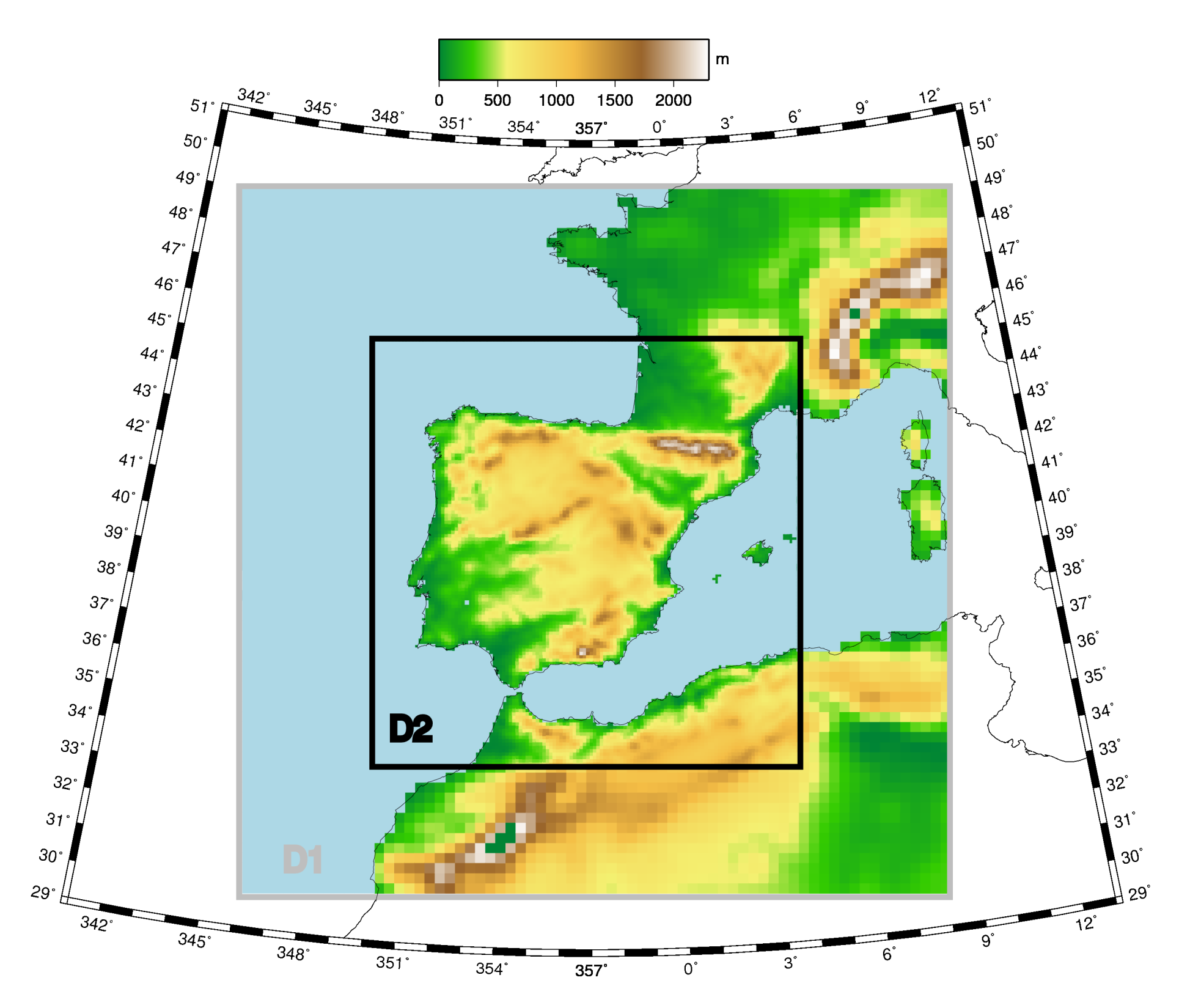
The spatial configuration consists of two-way nested domains with 30 and 10 km horizontal resolution respectively (Figure 1) and 24 sigma levels in the vertical up to 100 mb. ERA-Interim reanalysis [36] are used to provide initial and boundary condition which are updated every six hours. The physics configuration consist of Grell cumulus scheme [37], Simple Ice for microphysics [38], Rapid Radiative Transfer Model (RRTM) radiation scheme [39] and the Medium-Range Forecast (MRF) Planet Boundary Layer parameterization [40].

The runs have been performed for the year 1995 (considered as a dry year) with 4 additional months of spin-up period. This spin-up period guarantee that soil variables reach a dynamical equilibrium [41]. The RCM used here, employing similar configurations, has proved to provided satisfactory results while simulating the climate over the IP [25,42,43,44,45].

3. Results

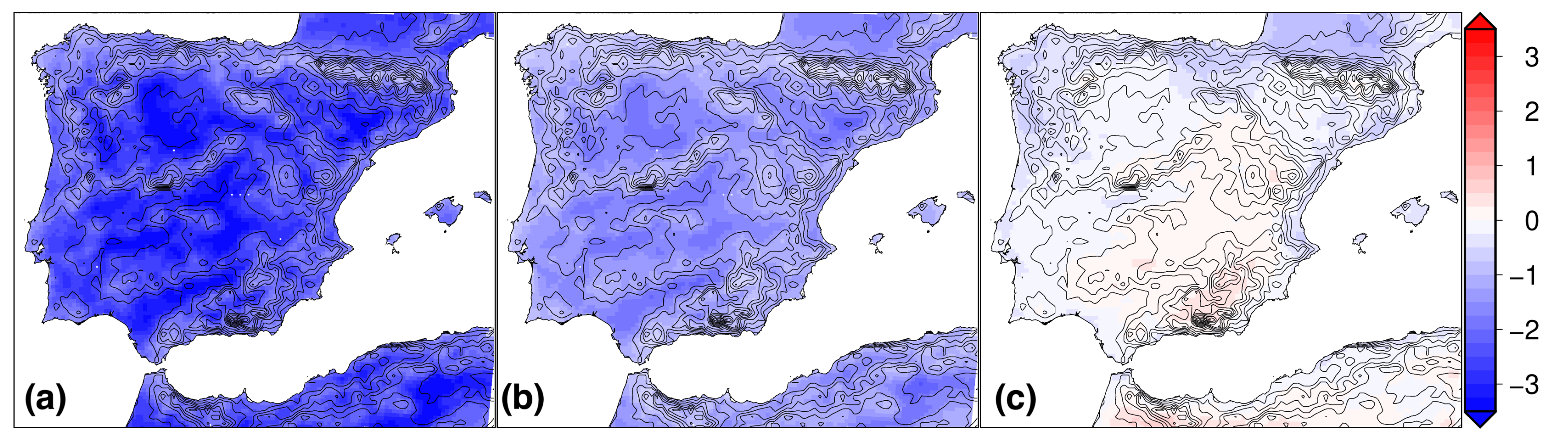
The analysis of differences (FCV90-FVC30) of the averaged minimum, mean and maximum temperature over the whole year (see Figure 2) shows that the temperature in the simulation with the highest FVC is always colder. The differences range from 0.2 to 2.2 ${}^{\circ }$C. The pattern of differences reveals that the greatest changes occurs in the valleys of the great rivers and inland flat areas. In the case of maximum temperatures, the differences present a spatial pattern characterized by a positive change in the south-east half of the domain and a negative change in the North of the domain, with differences ranging between −0.5 and 0.5 ${}^{\circ }$C. For minimum temperatures, the spatial pattern of the differences is very similar to that of mean temperatures but much more intense, with differences reaching 4 ${}^{\circ }$C. The spatial pattern of minimum temperature differences is related with the places where the denser cold air accumulates by gravity drainage. Meanwhile, the pattern of maximum temperature differences fits wet and dry areas. However, there is a large spatial variability along the year of such patterns. In summer, coastal Mediterranean areas show negative differences instead of the expected positive differences. This can be due to the enhancement of sea-breeze circulation related to the higher maximum temperatures inland. It is worth mentioning that the model has an idealized homogeneous land cover (cropland), which also explains the reasonably homogeneous patterns of the differences.

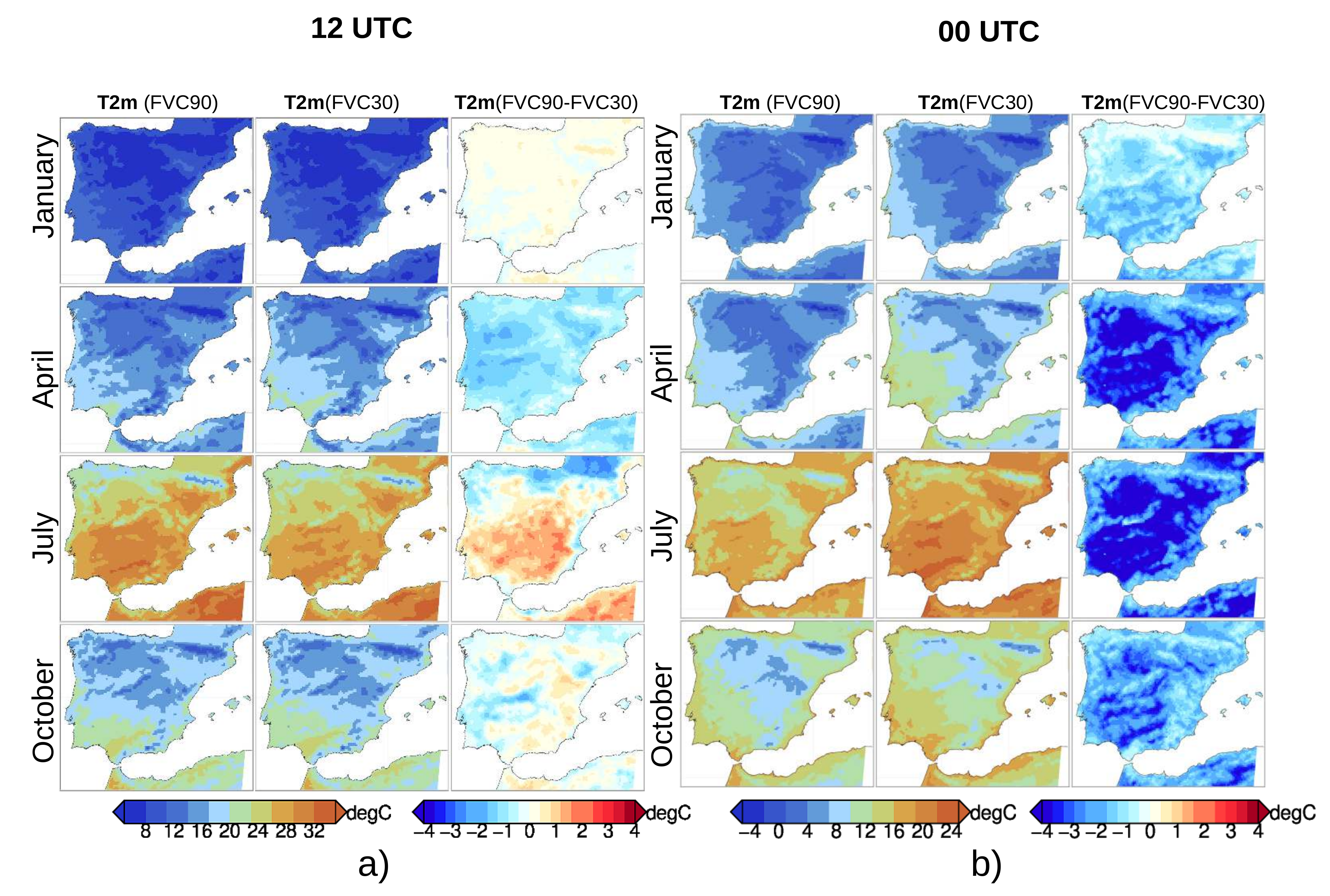
Below, we analyze the sensitivity to FVC for different times of the year and hours of the day. Figure 3 shows the air temperature at 2 m (T2m) at noon (12 UTC) (Figure 3a) and midnight (00 UTC) (Figure 3b) for each experiment and their differences for the central month of each season.

At night the difference patterns are almost the same along the year. They are coincident with the minimum temperature pattern shown above. However, the intensity depends on the time of the year, being much larger in summer (up to 5 ${}^{\circ }$C) that in winter (up to 1 ${}^{\circ }$C). On the other hand, the temperature difference patterns at midday strongly change along the year. In winter, temperature differences are small, in Spring are negative in all areas, while in Summer and Autumn some important differences appear between the north (negative) and south (positive) of the domain. Therefore, the effect of changing FVC on temperature is quite variable and depends on the time of day and season as well as on the surface properties.

3.1. Analysis of Surface Energy Fluxes

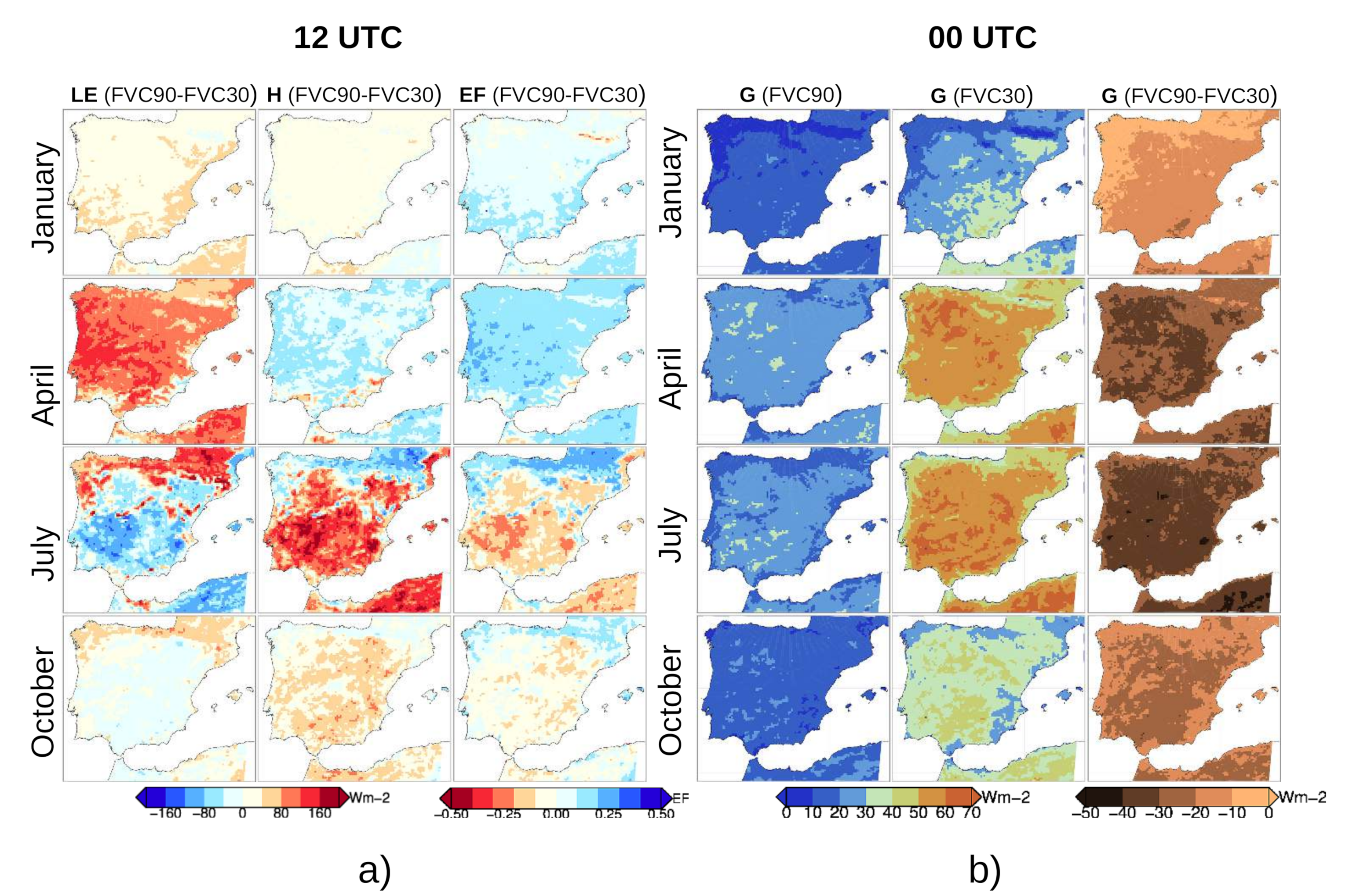
During the day, the temperature variations depend on the partitioning between H and LE. Figure 4a shows the differences between FVC90 and FVC30 for LE, H and EF at midday. During January and specially in April, LE is higher in FVC90, leading to lower values of H in most parts of the domain. However, this behaviour reverses in July and October in all areas of the domain but in the North. The obtained patterns correlate well with the changes obtained for maximum temperature (Figure 3a) and temperature at mid-day (Figure 3b). The spatial correlation with the differences of the sensible heat fluxes are 0.0 for January, 0.89 for April 0.89, 0.87 for July and 0.65 for October.

During the night, temperature changes depend on the availability of the soil for providing energy through G. Figure 4b depicts the surface fields of G at midnight. At first glance, it is clearly noticeable that upwards fluxes of this variable are always greater in the FVC30 experiment, primarily in July, with differences around 30–40 W/m${}^2$. As mentioned before, this difference in the ground heat fluxes comes from the lower $K_t$ in vegetated surfaces. During the day, the ground catches more energy (higher soil temperature) and during the night there is more heat available, besides heat can be released more easily to the atmosphere.

3.2. Canopy Resistance and Soil Moisture

As commented before, the main differences in maximum temperatures are related to the evaporative fraction. Let’s analyse them the canopy resistance as well as the soil moisture.

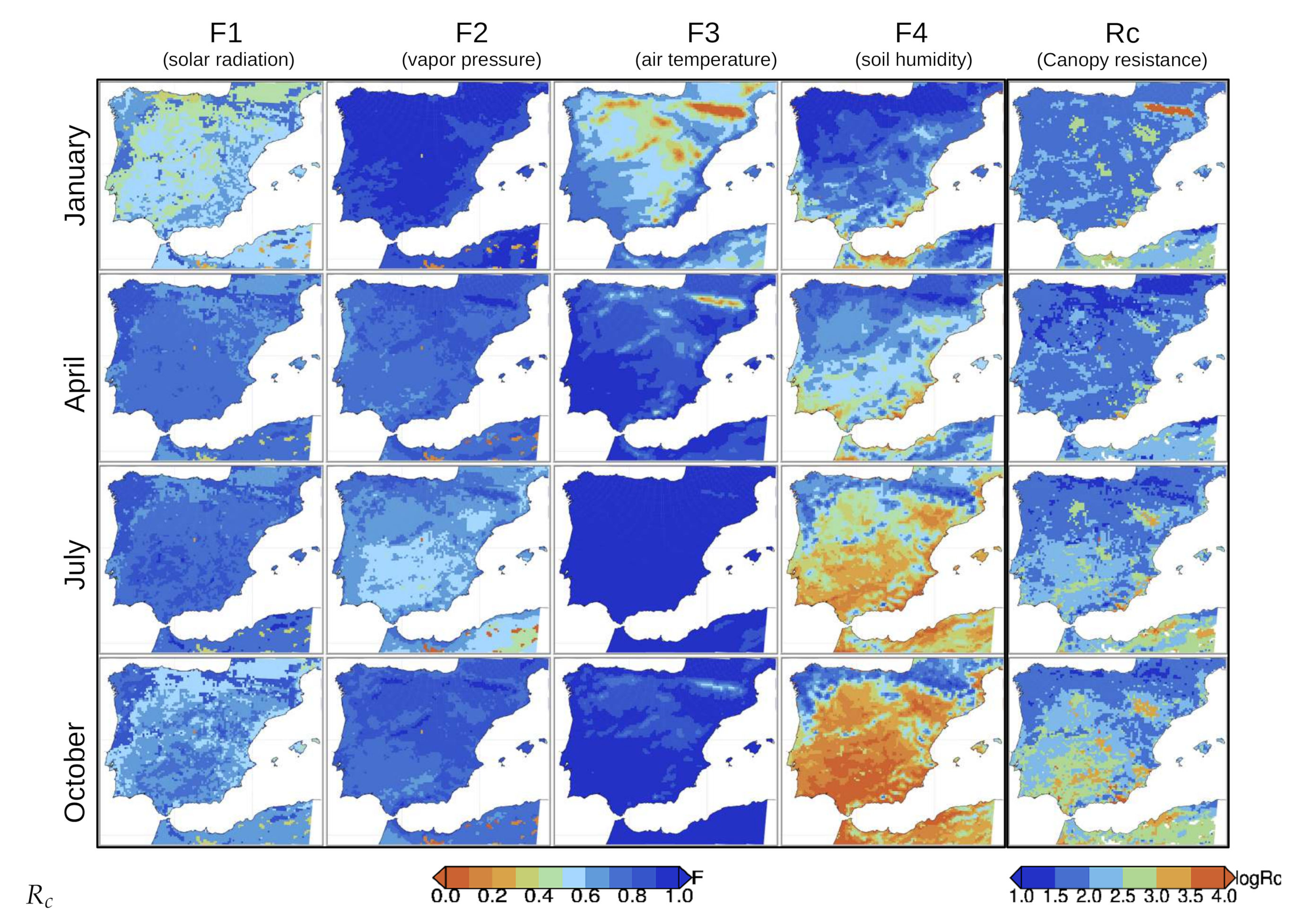
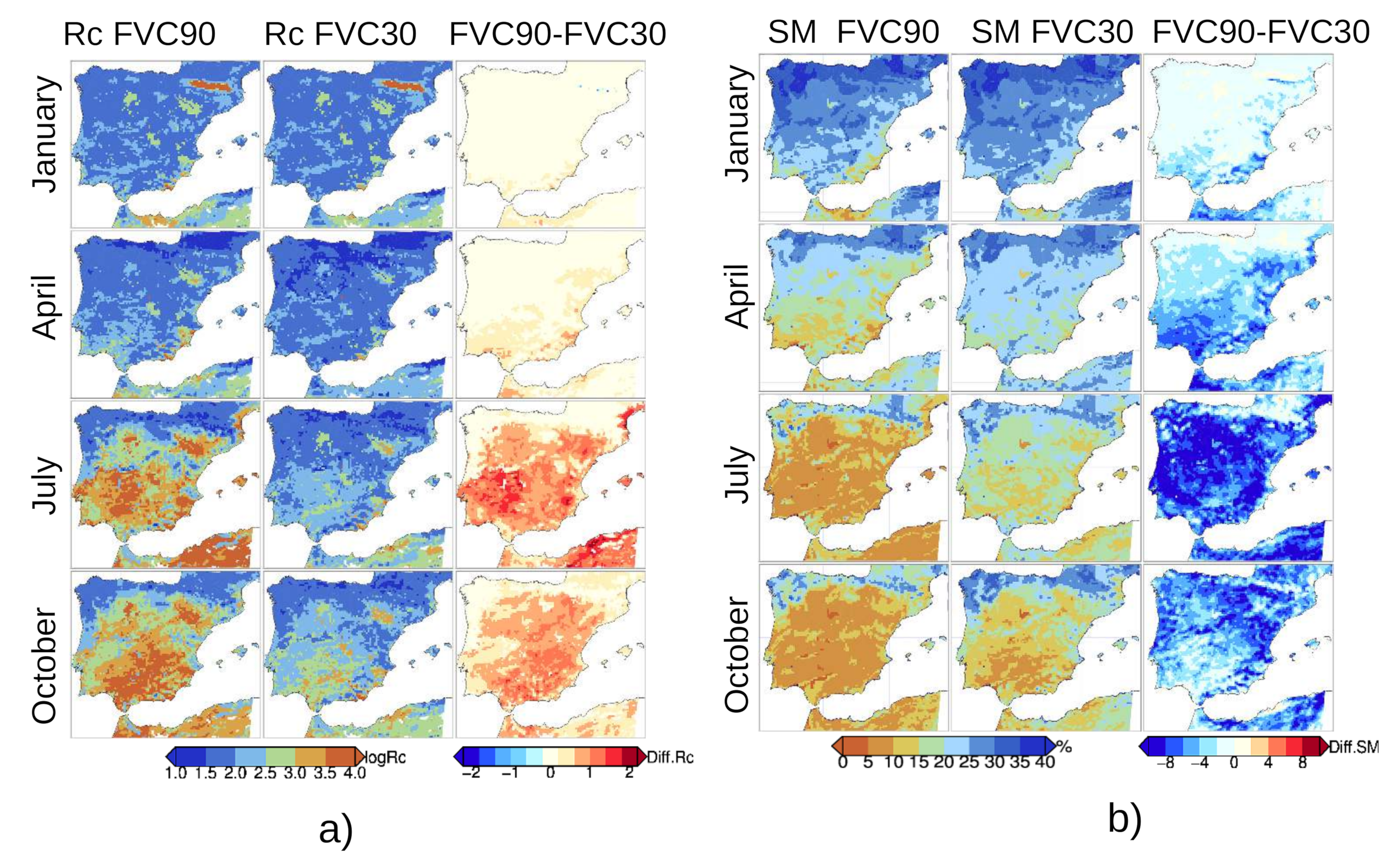
Figure 5 show the $R_c$ (expressed as logarithmic values) and the factors implied in its calculation for FVC30 experiment. The main contribution clearly comes from SM deficit (F4) with values very close to 0, showing a great difference respect the other factors. The FVC90 experiment presents a similar behaviour, being F4 lower, and therefore larger values of $R_c$ (not shown). The analysis of the $R_c$ (logarithmic) for FVC30, FVC90 and their differences (Figure 6a) displays that $R_c$ evolves along the year with a minimum in Spring and a maximum in October. $R_c$ is always higher in FVC90 and the differences are greater in summer, being the spatial pattern quite similar to the temperature differences at noon.

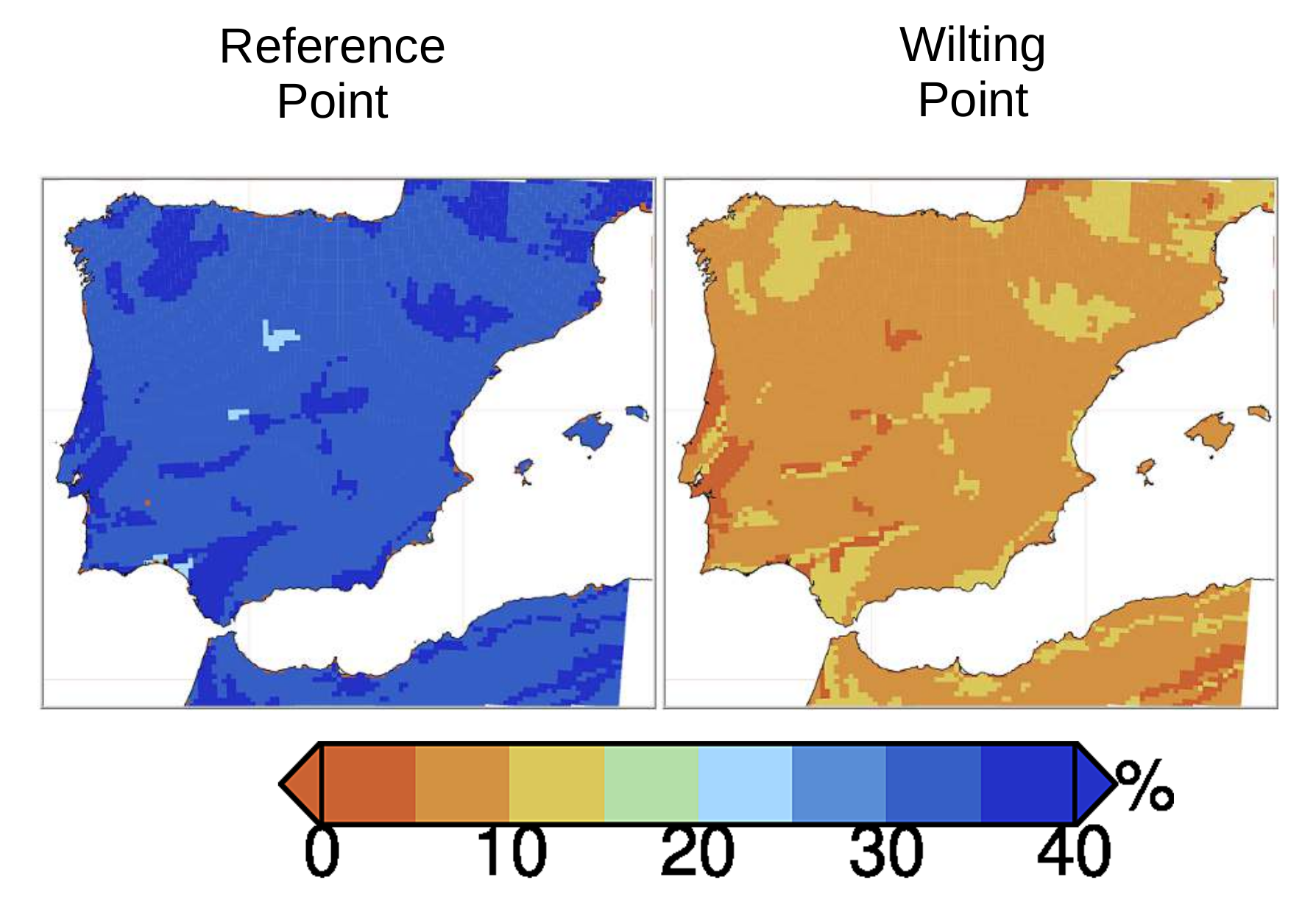
Regarding the SM, Figure 6b displays the monthly means for experiments FVFC30 and FVC90, and their differences for January, April, July and October for the third layer (from 0.6 to 1 m depth). This is the deepest layer that can provide water to vegetation. In this year, the soil moisture is decreasing along the year in both experiments reaching the wilting point in a large portion of the domain (see Figure 7). However, the drying of soil is faster in FVC90. Negative differences of SM appears everywhere along the whole year. Greater FVC (FVC90) leads to a higher extraction of SM for $E_t$ in the root zone layers. These differences reach its maximum in Summer (till 10%). Therefore the wilting point (WP), starting point when transpiration stops (Figure 7), is reached earlier in time and wider areas in FVC90 experiment. In addition, there is a reduction of the SM differences in October. This can be attributed to the fact of FVC90 experiment reaches before the WP and FVC30 can continue extracting water from soil.

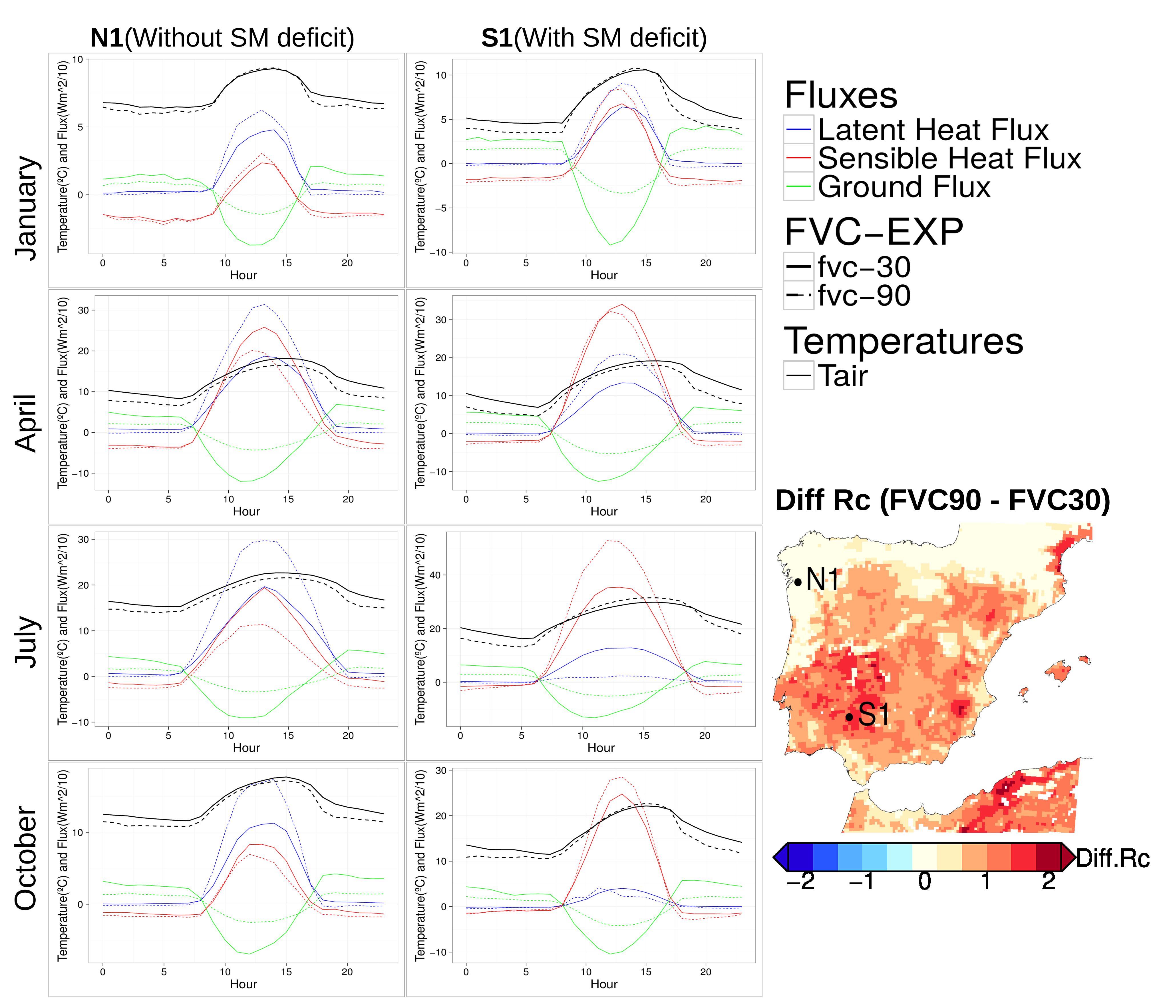
Therefore, the changes in temperature related to FVC mainly depend on the time of day and the availability of soil water. Figure 8 shows a clear example of this. We analyze the daily cycles of temperature and heat fluxes for the two simulations at two points (N1 and S1, see Figure 8) with very different water regimes. N1 is located in one area where there is not SM deficit along the year and there is just a slightly difference in $R_c$ between FVC90 and FVC30. The location of S1 presents a SM deficit and $R_c$ is much greater in FVC90 experiment.

Concerning nigh-time temperature, T2m is consistently minor in FVC90 for both locations, as a result of G being lower throughout the night in this experiment. This is linked with the reduction of $K_t$ in presence of vegetation, inhibiting the release of energy from soil layers to surface.

In N1, FVC30 T2m is always higher, but in winter, when temperature in both experiments is almost equal during the day. In this case, although LE flux is higher, H flux is also higher, due to the greater availability of energy due to the lower absorption by the soil. The differences in the heat transferred to the soil are quite similar along the year, while the amount of available energy is quite different depending on the season. This causes that H to be larger in FVC30 in the rest of seasons, leading to higher temperatures. It is also interesting that temperature differences between the experiments occur late in the afternoon and early at night. This is coincident with the maximum differences of upward ground heat flux.

In S1, the behaviour is similar while R_c difference is small (Winter and Spring). However, in Summer, LE is smaller in FVC90, leading to larger H and therefore to higher temperature. This LE depletion is associated to the SM deficit and R_c in FVC90 experiment. The effect of the higher vegetation coverage in FVC90 is a greater transpiration (LE fluxes) when SM is not a limiting factor. This greater evaporation entails a greater SM extraction from soil layers. Thereby, the WP is reached before in FVC90 that in FVC30 and this leads to a reversion of the cooling effect of vegetation (see Figure 9). Therefore, FVC90 shows higher temperature during the day, and lower temperatures during the night when soil moisture is scarce and transpiration is inhibited, leading to a bigger temperature daily range.

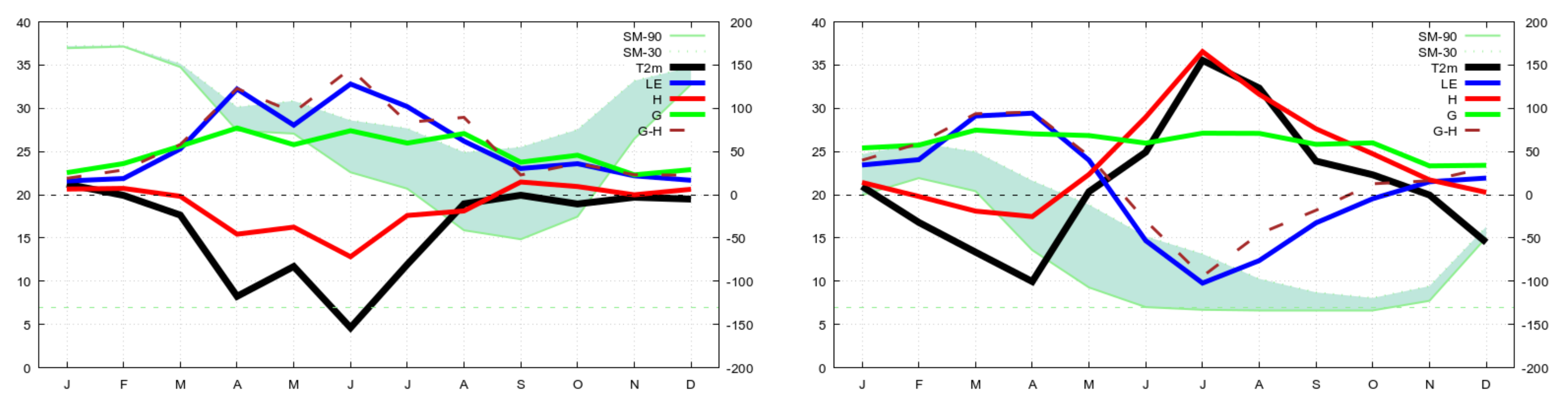
The different behaviour of both locations along the year at midday is presented in Figure 9. N1 is characterized by almost saturated soil in winter that evolves along the year with a minimum around September. The values for FVC90 are always lower but SM is always far from the WP. Temperature differences are negative, i.e., FVC90 shows lower temperatures, specially in summer, when differences reach 1.5 ${}^{\circ }$C. The colder temperature is due to the higher LE in FVC90 because the larger capacity for extracting water from soil. The behaviour in S1 is similar to N1 during the first months (from January to May). However, after May SM of FVC90 experiment reaches the WP. At this point, LE strongly decays leading to higher H that carries out higher temperatures. Note that in both locations, G flux is always larger in FVC30 leading to (G–H) differences perfectly fits to LE.

4. Discussion

In this work has been studied the sensitivity of temperature to changes of the FVC in a RCM coupled to the Noah LSM. The analysis was performed by carrying out two identical simulations of one full year with constant FVC (90 and 30%) for all land points of the domain and times of the year. Our results, show how temperature is modified by changes in FVC depending on the time of the year, the time of the day and soil moisture availability.

Increasing the FVC leads to decrease the thermal soil conductivity [17]. This implies a reduction of ground heat fluxes. During the day the soil absorbs less heat and therefore more sensible heat is available to warm the air. The final effect on temperature will depend on the portion of such sensible and latent heat fluxes ratio and will be discussed later. During the night the upward ground heat flux is diminished having as consequence a faster cooling of the air. Therefore, during the night a larger FVC always causes cooling.

When soil moisture is available, a FVC increase causes higher latent heat release through evapotranspiration. Therefore, during the day a larger FVC cools the air. The final effects on temperature will depend on the excess of sensible heat mentioned above related to the soil thermal conductivity. On the other hand, changes in FVC leads to changes of a stress term in the canopy resistance parameterization [15] mainly trough the soil moisture availability. Under high moisture stress, soil moisture near the WP, the latent heat released by evapotranspiration is strongly diminished, therefore such cooling effect almost disappears. This originates that an increase of FVC does not modify latent heat flux in such conditions.

As mentioned before, larger FVC leads to a faster drying of soil which implies larger effects on canopy resistance. High canopy resistance values inhibits water flux transpiration. In a situation of scarce precipitation, a soil with higher FVC reaches the Wilting Point before a less vegetated soil. This leads to have less latent heat, occasioning higher diurnal temperatures.

This response was also analyzed by [18] while comparing simulations with fixed and dynamic FVC studying North American monsoons. They also indicate the relevance of soil moisture factor in their simulations and the fact that higher FVC not always enhances EF and $E_t$. Other authors also highlight the importance of canopy resistance physics in controlling evaporation [9,46].

5. Conclusions

Summarizing, increasing FVC always entails lower temperatures at night. The maximum cooling occurs in places where cold air is accumulated (valleys, plane areas, etc). If soil moisture is available, increasing FVC leads to a drop in temperature when the excess of latent heat by evapotranspiration is larger that the excess of sensible heat due to the lesser thermal soil conductivity. In winter months both almost compensate and diurnal temperatures do not suffer great changes. However, in the rest of the year latent heat flux is larger and air temperature decreases. In case of dry soils, latent heat becomes small and temperature increases. In addition, more vegetation leads to faster drying of the soils, reaching the WP before and provoking higher temperatures.

Note that this behavior is related with an increase of the daily temperature range. In the case of our experiments, the mean annual differences over land are larger than 2 ${}^{\circ }$C, reaching some specific places at some months values above 5 ${}^{\circ }$C when changing FVC from 30 to 90%. It is worth mentioning that results can be model dependent, therefore it would be desirable to perform more experiments using other LSMs based on varied physical approaches.

Thus, we find a remarkable sensitivity of temperature to FVC. The FVC variations imposed in our experiments could serve as an upper limit to the common differences that can be found due to different factors such as inter-annual variability, reconstruction method of FVC, NDVI databases, etc. Therefore, a correct estimation of FVC values is crucial in order to improve temperature representation in RCMs. Moreover, the canopy resistance parameterization is critical in understanding the final effect of FVC [18], then a correct representation of canopy resistance parameters like $R_{cmin}$ [47] or parameters dependent of soil type could have a non-negligible impact on RCM experiments.

Another important aspect may be the impact that the imposition of future vegetation values may have on climate change scenarios. An excess of vegetation in areas where future projections tend to give drier climates may amplify the estimates of increase in maximum temperatures, with the consequent effect on heat waves. One interesting question may be related to a better understanding of compound events such as droughts and fires. Areas with large vegetation in situations of water stress can cause temperatures to rise more and in turn make droughts more extreme increasing the probability of fires. On the other hand, a future reduction of vegetation might lead to an increase of temperature, specially the minimum ones, favoring extreme events such as raising the number of tropical nights.

References

- Dickinson, R.E.; Henderson-Sellers, A. Modelling tropical deforestation: A study of GCM land-surface parametrizations. Quart. J. Roy. Meteor. Soc. 1988, 114, 439–462. [Google Scholar] [CrossRef]
- Foley, J.A.; Prentice, I.C.; Ramankutty, N.; Levis, S.; Pollard, D.; Sitch, S.; Haxeltine, A. An integrated biosphere model of land surface processes, terrestrial carbon balance, and vegetation dynamics. Glob. Biogeoch. Cycles 1996, 10, 603–628. [Google Scholar] [CrossRef]
- Costa, M.; Pires, G.F. Effects of Amazon and Central Brazil deforestation scenarios on the duration of the dry season in the arc of deforestation. Int. J. Climatol. 2010, 30, 1970–1979. [Google Scholar] [CrossRef]
- Copeland, J.H.; Pielke, R.A.; Kittel, T.G. Potential climatic impacts of vegetation change: A regional modeling study. J. Geophys. Res. Atmos. 1996, 101, 7409–7418. [Google Scholar] [CrossRef]
- Heck, P.; Lüthi, D.; Wernli, H.; Schär, C. Climate impacts of European-scale anthropogenic vegetation changes: A sensitivity study using a regional climate model. J. Geophys. Res. Atmos. 2001, 106, 7817–7835. [Google Scholar] [CrossRef]
- Müller, O.V.; Berbery, E.H.; Alcaraz-Segura, D.; Ek, M.B. Regional model simulations of the 2008 drought in southern South America using a consistent set of land surface properties. J. Clim. 2014, 27, 6754–6778. [Google Scholar] [CrossRef] [Green Version]
- Xu, L.; Pyles, R.D.; Snyder, R.; Monier, E.; Falk, M.; Chen, S.H. Impact of canopy representations on regional modeling of evapotranspiration using the WRF-ACASA coupled model. Agric. For. Meteor. 2017, 247, 79–92. [Google Scholar] [CrossRef] [Green Version]
- Segal, M.; Avissar, R.; Pielke, M.M.R. Evaluation of vegetation effects on the generation and modification of mesoscale circulations. J. Atmos. Sci. 1988, 45, 2268–2292. [Google Scholar] [CrossRef] [Green Version]
- Kurkowski, N.P.; Stensrud, D.J.; Baldwin, M.E. Assessment of Implementing Satellite-Derived Land Cover Data in the Eta Model. Wea. Forecast. 2003, 18, 404–416. [Google Scholar] [CrossRef] [Green Version]
- Vahmani, P.; Ban-Weiss, G. Impact of remotely sensed albedo and vegetation fraction on simulation of urban climate in WRF-urban canopy model: A case study of the urban heat island in Los Angeles. J. Geophys. Res. 2016, 121, 1511–1531. [Google Scholar] [CrossRef]
- Stensrud, D.J. Parameterization Schemes: Keys to Understanding Numerical Weather Prediction Models; Cambridge University Press: Cambridge, UK, 2007. [Google Scholar]
- Jiménez-Gutiérrez, J.M.; Valero, F.; Jerez, S.; Montávez, J.P. Impacts of green vegetation fraction derivation methods on regional climate simulations. Atmosphere 2019, 10, 281. [Google Scholar] [CrossRef] [Green Version]
- Carlson, T.N.; Rypley, D.A. On the relation between NDVI, fractional vegetation cover, and leaf area index. Remote Sens. Environ. 1997, 62, 241–252. [Google Scholar] [CrossRef]
- Montandon, L.M.; Small, E.E. The impact of soil reflectance on the quantification of the green vegetation fraction from NDVI. Remote Sens. Environ. 2008, 112, 1835–1845. [Google Scholar] [CrossRef]
- Jacquemin, B.; Noilhan, J. Sensitivity study and validation of a land surface parameterization using the HAPEX-MOBILHY data set. Bound. Lay. Meteor. 1990, 52, 93–134. [Google Scholar] [CrossRef]
- Hong, S.; Lakshmi, V.; Small, E.; Chen, F.; Tewari, M.; Manning, K.W. Effects of vegetation and soil moisture on the simulated land surface processes from the coupled WRF/Noah model. J. Geophys. Res. Atmos. 2009, 114. [Google Scholar] [CrossRef]
- Ek, M.B.; Mitchell, K.E.; Lin, Y.; Rogers, E.; Grunmann, P.; Koren, V.; Gayno, G.; Tarpley, J.D. Implementation of Noah land surface model advances in the National Centers for Environmental Prediction operational mesoscale Eta model. J. Geophys. Res. Atmos. 2003, 108. [Google Scholar] [CrossRef]
- Matsui, T.; Lakshmi, V.; Small, E.E. The effects of satellite-derived vegetation cover variability on simulated land-atmosphere interactions in the NAMS. J. Clim. 2005, 18, 21–40. [Google Scholar] [CrossRef]
- Gutman, G.; Ignatov, A. The derivation of the green vegetation fraction from NOAA/AVHRR data for use in numerical weather prediction models. Int. J. Remote Sens. 1998, 19, 1533–1543. [Google Scholar] [CrossRef]
- Refslund, J.; Dellwik, E.; Hahmann, A.; Barlage, M.; Boegh, E. Development of satellite green vegetation fraction time series for use in mesoscale modeling: Application to the European heat wave 2006. Theor. App. Clim. 2014, 117, 377–392. [Google Scholar] [CrossRef] [Green Version]
- James, K.A.; Stensrud, D.J.; Yussouf, N. Value of real-time vegetation fraction to forecasts of severe convection in high-resolution models. Wea. Forecast. 2009, 24, 187–210. [Google Scholar] [CrossRef]
- Meng, X.H.; Evans, J.P.; McCabe, M.F. The Impact of Observed Vegetation Changes on Land–Atmosphere Feedbacks During Drought. J. Hydrometeor. 2014, 15, 759–776. [Google Scholar] [CrossRef] [Green Version]
- Crawford, T.M.; Stensrud, D.J.; Mora, F.; Merchant, J.W.; Wetzel, P.J. Value of Incorporating Satellite-Derived Land Cover Data in MM5/PLACE for Simulating Surface Temperatures. J. Hydrometeor. 2001, 2, 453–468. [Google Scholar] [CrossRef]
- Tullot, I.F. Climatología de España y Portugal; Universidad de Salamanca: Salamanca, Spain, 2000; Volume 76. [Google Scholar]
- Lorente-Plazas, R.; Montávez, J.; Jerez, S.; Gómez-Navarro, J.; Jiménez-Guerrero, P.; Jiménez, P. A 49 year hindcast of surface winds over the Iberian Peninsula. Int. J. Climatol. 2015, 35, 3007–3023. [Google Scholar] [CrossRef]
- Chen, F.; Dudhia, J. Coupling an advanced land-surface/hydrology model with the Penn State/NCAR MM5 modeling system. Part I: Model implementation and sensitivity. Mon. Wea. Rev. 2001, 129, 569–585. [Google Scholar] [CrossRef] [Green Version]
- Grell, G.; Dudhia, J.; Stauffer, D. A description of the fifth-generation Penn State/NCAR Mesoscale Model (MM5). Ncar Tech. Note NCAR 1994, NCAR-TN-398 +STR. 117. [Google Scholar] [CrossRef]
- Mahrt, L.; Ek, M. The influence of atmospheric stability on potential evaporation. J. Appl. Meteor. 1984, 23, 222–234. [Google Scholar] [CrossRef] [Green Version]
- Mahrt, L.; Pan, H. A two-layer model of soil hydrology. Bound. Lay. Meteor. 1984, 29, 1–20. [Google Scholar] [CrossRef]
- Pan, H.L.; Mahrt, L. Interaction between soil hydrology and boundary-layer development. Bound. Lay. Meteor. 1987, 38, 185–202. [Google Scholar] [CrossRef]
- Chen, F.; Mitchell, K.; Schaake, J.; Xue, Y.; Pan, H.L.; Koren, V.; Betts, A. Modeling of land surface evaporation by four schemes and comparison with FIFE observations. J. Geophys. Res. Atmos. 1996, 101, 7251–7268. [Google Scholar] [CrossRef] [Green Version]
- Noilhan, J.; Planton, S. A simple parameterization of land surface processes for meteorological models. Mon. Wea. Rev. 1989, 117, 536–549. [Google Scholar] [CrossRef]
- Ek, M.; Mahrt, L. OSU 1-D PBL Model User’s Guide; Technical Report; Department of Atmospheric Sciences, Oregon State University: Corvallis, OR, USA, 1991. [Google Scholar]
- Peters-Lidard, C.D.; Zion, M.S.; Wood, E.F. A soil-vegetation-atmosphere transfer scheme for modeling spatially variable water and energy balance processes. J. Geophys. Res. Atmos. 1997, 102, 4303–4324. [Google Scholar] [CrossRef]
- Mahfouf, J.F.; Noilhan, J. Comparative study of various formulations of evaporations from bare soil using in situ data. J. Appl. Meteor. 1991, 30, 1354–1365. [Google Scholar] [CrossRef] [Green Version]
- Dee, D.P.; Uppala, S.M.; Simmons, A.; Berrisford, P.; Poli, P.; Kobayashi, S.; Andrae, U.; Balmaseda, M.A.; Balsamo, G.; Bauer, P.; et al. The ERA-Interim reanalysis: Configuration and performance of the data assimilation system. Q. J. R. Meteor. Soc. 2011, 137, 553–597. [Google Scholar] [CrossRef]
- Grell, G.A. Prognostic evaluation of assumptions used by cumulus parameterizations. Mon. Wea. Rev. 1993, 121, 764–787. [Google Scholar] [CrossRef] [Green Version]
- Dudhia, J. Numerical study of convection observed during the winter monsoon experiment using a mesoscale two-dimensional model. J. Atmos. Sci. 1989, 46, 3077–3107. [Google Scholar] [CrossRef]
- Mlawer, E.; Taubman, S.; Brown, P.; Iacono, M.; Clough, S. Radiative transfer for inhomogeneous atmospheres: RRTM, a validated correlated-k model for the longwave. J. Geophys. Res. 1997, 102, 16663–16682. [Google Scholar] [CrossRef] [Green Version]
- Hong, S.; Pan, H. Nonlocal boundary layer vertical diffusion in a Medium-Range Forecast Model. Mon. Wea. Rev. 1996, 124, 2322–2339. [Google Scholar] [CrossRef] [Green Version]
- Jerez, S.; López-Romero, J.M.; Turco, M.; Lorente-Plazas, R.; Gómez-Navarro, J.J.; Jiménez-Guerrero, P.; Montávez, J.P. On the Spin-Up Period in WRF Simulations Over Europe: Trade-Offs Between Length and Seasonality. J. Adv. Model. Earth Syst. 2020, 12, e2019MS001945. [Google Scholar] [CrossRef] [Green Version]
- Jerez, S.; Montavez, J.P.; Gomez-Navarro, J.J.; Jimenez-Guerrrero, P.; Jimenez, J.M.; Gonzalez-Rouco, J.F. Temperature sensitivity to the land-surface model in MM5 climate simulations over the Iberian Peninsula. Meteor. Z. 2010, 19, 363–374. [Google Scholar] [CrossRef] [Green Version]
- Gómez-Navarro, J.; Montávez, J.; Jiménez-Guerrero, P.; Jerez, S.; Lorente-Plazas, R.; González-Rouco, J.; Zorita, E. Internal and external variability in regional simulations of the Iberian Peninsula climate over the last millennium. Clim. Past 2012, 8, 25. [Google Scholar] [CrossRef] [Green Version]
- Jerez, S.; Montavez, J.P.; Jimenez-Guerrero, P.; Gomez-Navarro, J.J.; Lorente-Plazas, R.; Zorita, E. A multi-physics ensemble of present-day climate regional simulations over the Iberian Peninsula. Clim. Dyn. 2013, 40, 3023–3046. [Google Scholar] [CrossRef]
- Fernández-Montes, S.; Gómez-Navarro, J.; Rodrigo, F.; García-Valero, J.; Montávez, J. Covariability of seasonal temperature and precipitation over the Iberian Peninsula in high-resolution regional climate simulations (1001–2099). Glob. Planet. Chang. 2017, 151, 122–133. [Google Scholar] [CrossRef]
- Marshall, C.H.; Crawford, K.C.; Mitchell, K.E.; Stensrud, D.J. The impact of the land surface physics in the operational NCEP Eta model on simulating the diurnal cycle: Evaluation and testing using Oklahoma Mesonet data. Wea. Forecast. 2003, 18, 748–768. [Google Scholar] [CrossRef]
- Kumar, A.; Chen, F.; Barlage, M.; Ek, M.B.; Niyogi, D. Assessing impacts of integrating MODIS vegetation data in the weather research and forecasting (WRF) model coupled to two different canopy-resistance approaches. J. Appl. Meteor. Climatol. 2014, 53, 1362–1380. [Google Scholar] [CrossRef]
Figure 1.
RCM spatial domains. Mother domain, D1 (30 km), and inner domain, D2 (10 km). Topography of the spatial domains.
Figure 2.
Differences between FVC90-FVC30 experiment for (a) minimum, (b) mean, and (c) maximum daily temperature (°C) averaged over the whole period. Black contours denote the topography.
Figure 3.
T2m (°C) for experiments FVC90 and FVC30 and their differences at 12 UTC (a) and at 00 UTC (b) for January, April, July and October.
Figure 4.
(a) Differences of LE (W/m2), H (W/m2) and EF between experiments FVC90 and FVC30 at 12 UTC. (b) G (W/m2) for experiments FVC90 and FVC30 and its differences at 00 UTC. Monthly means of January, April, July and October.
Figure 5.
Experiment FVC30. Deficit factors F1, F2, F3, F4 and Rc. Monthly means of January, April, July and October.
Figure 6.
(a) Rc for experiments FVC90 and FVC30 and its differences. (b) SM (%) (0.6–1 m depth) for experiments FVC90 and FVC30 and its differences. Monthly means of January, April, July and October.
Figure 7.
Wilting point and Reference Point for SM (%).
Figure 8.
Hourly means averaged for January, April, July and October. T2m (black line), H (red line), LE (blue line) and G (green line) for experiments FVC90 (dashed line) and FVC30 (solid line). Representative locations without SM deficit (N1) and with SM deficit (S1).
Figure 9.
Monthly mean differences at midday between FVC90 and FVC30 experiments for temperature (°C × 102) and latent, sensible and ground heat fluxes (W/m2, left y-axis). Shaded green area represents the differences of the soil moisture at the third layer of the soil model (%, right y-axis). FVC90 has always the lower value. The constant dashed green-light line represents the wilting point. Left (right) panel shows the results for N1 (S1).
Publisher’s Note: MDPI stays neutral with regard to jurisdictional claims in published maps and institutional affiliations. |
© 2021 by the authors. Licensee MDPI, Basel, Switzerland. This article is an open access article distributed under the terms and conditions of the Creative Commons Attribution (CC BY) license (https://creativecommons.org/licenses/by/4.0/).
Share and Cite
MDPI and ACS Style
Jiménez-Gutiérrez, J.M.; Valero, F.; Ruiz-Martínez, J.; Montávez, J.P. Temperature Response to Changes in Vegetation Fraction Cover in a Regional Climate Model. Atmosphere 2021, 12, 599. https://doi.org/10.3390/atmos12050599
AMA Style
Jiménez-Gutiérrez JM, Valero F, Ruiz-Martínez J, Montávez JP. Temperature Response to Changes in Vegetation Fraction Cover in a Regional Climate Model. Atmosphere. 2021; 12(5):599. https://doi.org/10.3390/atmos12050599
Chicago/Turabian StyleJiménez-Gutiérrez, Jose Manuel, Francisco Valero, Jesús Ruiz-Martínez, and Juan Pedro Montávez. 2021. "Temperature Response to Changes in Vegetation Fraction Cover in a Regional Climate Model" Atmosphere 12, no. 5: 599. https://doi.org/10.3390/atmos12050599
Note that from the first issue of 2016, this journal uses article numbers instead of page numbers. See further details here.