Numerical Study on the Plume Behavior of Multiple Stacks of Container Ships

Abstract

This paper showed different plume behaviors of exhausts from different number of stacks of the container ship, using CFD code PHOENICS version 6.0. The plume behavior was quantitatively analyzed by mass fraction of the pollutant in the exhaust and plume heights. Three simplified typical configurations were constructed by CFD according to the investigation of container ships. The configurations included a single main stack (BL1), one main stack and multiple auxiliary stacks (BL2), and two main stacks and multiple auxiliary stacks (BL3). All the main stacks had the same emission characteristics, and all the auxiliary stacks had the same emission characteristics. The results show that the transmission and diffusion characteristics of the exhaust from multiple stacks are different from those of the exhaust from a single stack. In BL2 and BL3 simulations, the maximum mass fraction of SO₂ in the exhaust (C1_max) of multiple stack emissions was approximately 329% and 269% higher than that of single stack emissions over the main stack, respectively, and the plume height of multiple stack emissions is higher than that of single stack emissions. In BL2 and BL3 simulations, the plume height of multiple stack emissions was 41% and 75% higher than that of single stack emissions, respectively. The increase of C1_max, due to multiple stack emissions, is weakened as the distance of the stacks increase. The difference in plume behavior between multiple stack emissions and single stack emissions is of great significance for air quality management and pollution control in port areas.

1. Introduction

With the development of international trade and globalization, ship emissions have a significant impact on air pollution [1] and may influence the global and local environment, human health, and quality of life, especially in offshore and coastal areas [2,3,4,5,6]. Maritime trade accounted for more than 80% of global trade by the end of 2015 [7]. In the last few years, the total number of ships and ports in China has rapidly increased, making the regional pollution in port cities more serious [8]. Therefore, the increasing concentration of pollutants in port cities needs more attention [9,10], and ship pollution has become an important source.

The most common ship pollutants include carbon dioxide, nitrogen oxides, sulfur dioxide, carbon monoxide, hydrocarbons, and primary and secondary particles. Zhao et al. [11] monitored and analyzed the pollutant concentrations in Shanghai Ports and used the backward trajectory analysis to discover that SO₂ and NO₂ in coastal areas were mainly caused by ship emissions. Chen et al. [12] combined SMOKE/WRF/CMAQ (the Spare Matrix Operator Kernel Emissions/Weather Research and Forecast/Community Multiscale Air Quality model) with a ship emission inventory to show that N and S depositions in coastal and offshore areas contributed by ship emissions were more than 15 kg·ha⁻¹·yr⁻¹. Liu et al. [13] combined measurement results and WRF/CMAQ (the Weather Research and Forecasting/Community Multiscale Air Quality model) to determine that up to 20–30% (2–7µg/m³) of PM_2.5 concentration was generated by ship emissions in coastal and riverside areas of Shanghai.

Murena et al. [14] assessed the influence of cruise ship emissions on air quality in the port of Naples using CAILPUFF (the California Puff model) and compared the results with fixed monitoring data. The correlation between the measurement results and simulation results was low; the study attributed this to the fact that the pollutant sources of fixed monitoring points were more than those of ship simulation, which were limited in the seaside area.

Karla et al. [15] compared the results of CALPUFF with the measurement results and investigated the concentrations of PM_2.5, NO₂, and SO₂ contributed by ship emissions in James Bay, Victoria, British Columbia, Canada. The study reported that the results of CALPUFF were lower than measurement results, inferring that the ship model had not been effectively established and some unknown sources were not considered. In June 2018, we also found several special cases where the pollutant concentrations monitored by unmanned aerial vehicles were significantly higher than those simulated by WRF/CALPUFF, during a short-term observation period in Yantian Port, Shenzhen. A logical assumption was that the plume height of measurement results was significantly lower than that of simulation results due to the model setup, which was consistent with the reasons noted in [15].

The superstructure of the ship is an important factor in modeling, which may have a significant impact on the plume behavior. Vijayakumar et al. [16] conducted a wind tunnel study on the ship superstructure to investigate the interaction between the exhaust smoke and superstructure. The study found that the downwash would occur when the distance between the mast and the funnel was close. Kulkarni et al. [17] performed a wind tunnel study to assess the exhaust smoke–superstructure interaction on the ship. The study found that the exhaust smoke from two funnels, which had the same structure, had two different plume trajectories when the first funnel was in front of the second one. The exhaust from the first funnel disturbed the plume distribution of the second one. Park et al. [18] carried out CFD (the Computational Fluid Dynamics model) study to argue that ineffective funnel designs would influence the plume distribution and could damage the ship’s electronic equipment on the superstructure. Kulkarni et al. [19] investigated the interaction between the exhaust smoke and ship superstructures. The study compared the results of CFD with measurement results, demonstrating the usefulness of CFD as a tool to simulate the exhaust plume emitted from ship funnel.

Previous studies assumed that multiple stacks on container ships were a single whole unit, without considering that the plume behavior of the exhaust from multiple stacks may be different from that of the exhaust from a single stack, due to the concentrated release of hot smoke. This may lead to measurement errors in the study conducted on regional scale. Schulman and Scire [20] found that the plume height of exhaust from a single line source was much lower than that of exhaust from multiple line sources that were close to each other. The plume height was relative to the length and design of the line sources. Sumner et al. [21] showed that, compared to the turbulence flow around stacks of single stack emissions, the turbulence flow around stacks of two stack emissions showed a significant difference. The Environmental Protecting Research Institute at the Central Research Institute of Building and Construction in China [22] conducted a wind tunnel study to evaluate the plume height of exhaust emitted from two stacks that were close to each other. The study found that the plume height of exhaust emitted from two stacks was approximately 33% higher than that of exhaust emitted from a single stack. Therefore, further studies are needed to clarify the difference in exhaust plume behaviors between multiple stack emissions and single stack emissions.

In this study, three simplified stack configurations of container ships were established using CFD (the Computational Fluid Dynamics model). This paper further quantitative analyzes the difference in mass fraction of SO₂ in the exhaust and the exhaust plume height between single stack emissions and multiple stack emissions, providing technical support and theoretical basis for subsequent ship pollution simulation research.

2. Methods

2.1. Nomenclature

In this paper, qualitative analysis was showed in the results using some nomenclatures, as shown in

Table 1. Nomenclature.

C10-M1/A1	C1	C1max	C1max-M1/A1	C11km-M1	V wind
Mass fraction of SO2 in the exhaust from the stack at the outlet of the main/auxiliary stack	Mass fraction of SO2 in the plume	Maximum C1	The maximum C1 over the main stack on the M1/A1 plane	The maximum C1 at around 1 km downwind of the stack on the M1 plane	Wind speed

.

2.2. Physical Model Setup

In the present study, three typical simplified stack configurations were established to analyze the transport and distribution of SO₂ in the exhaust. The configurations selected were based on the investigation on 116 container ships in June 2018, in the Shenzhen port, Guangdong, China, as shown in

Table 2. Different stack configurations ¹ and the corresponding physical models.

	BL1(Single Main Stack)	BL2(A Main Stack and Multi- Auxiliary Stacks)	BL3(Two Main Stacks and Multi- Auxiliary Stacks)
Real ships
CFDModels

¹ Reference of ship models: http://www.shipxy.com/.

. The first configuration (BL1) was modeled on the ship GRETE MAERSK, consisting of a single main stack, as the ship exhaust was from a single stack. The second configuration (BL2) was modeled on the ship MSC LAURENCE, consisting of a main stack and six auxiliary stacks, located on either side of the main stack. The ship pollution was contributed by the main engine, auxiliary engine, and boiler. The third configuration (BL3) was modeled on the ship MATHILDE MAERSK and consisted of two main stacks and six auxiliary stacks. The lines in Table 1 marked M1, A1, and A2 are the centerlines of the main stacks and auxiliary stacks.

The diameters of the main stack and the auxiliary stack were 2.5 and 0.8 m, respectively. The distance between the main stack and the auxiliary stack was 1.75 m, and the distance between two main stacks was 9.5 m.

2.3. Computational Domain and Numberical Considerations

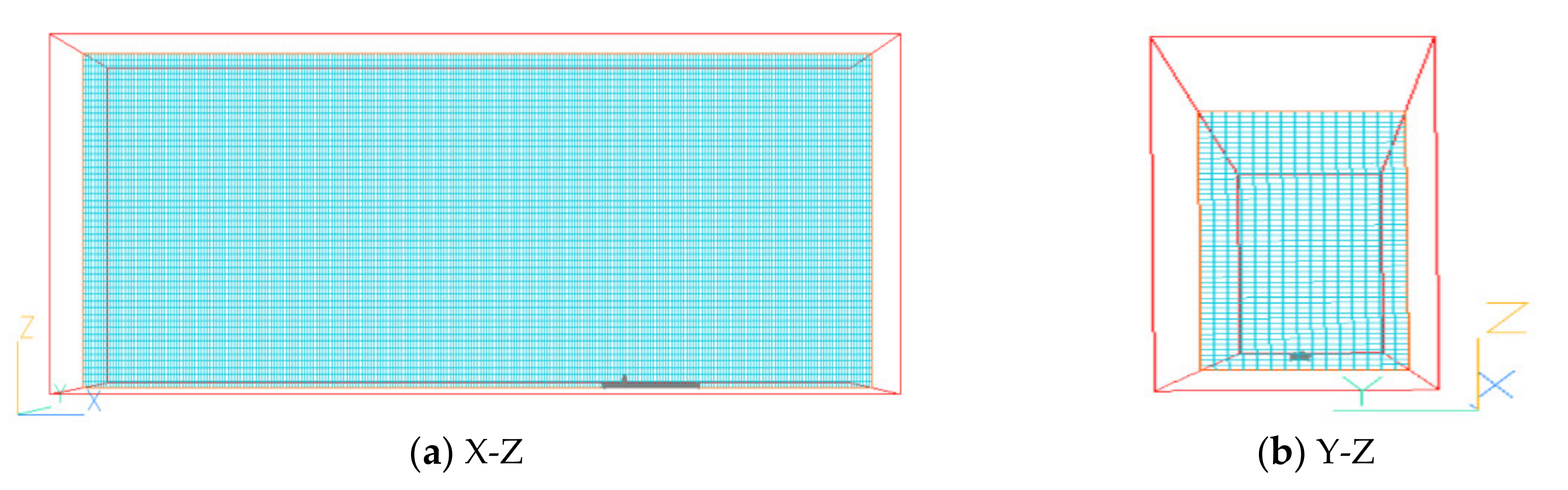
The computational domain covered a volume of 2600 (global x axis in this analysis) × 400 (global y axis in this analysis) × 1000 m (global z axis in this analysis). The dimension of the ship was 324 (length) × 43 (width) × 40 (height) m³. The structured grid was selected in this study, which was automatically generated after physical modeling. The mesh had 1,040,000 tetrahedral cells, as shown in Figure 1.

The standard k-ε turbulence model was used in the CFD (PHOENICS version 6.0) modeling. The boundary conditions, initial conditions, governing equations, and some other assumptions are shown in

Table 3. Boundary conditions, initial conditions, governing equations, and extra assumptions.

Boundary conditions	All solid surfaces were set as non-slip conditions. In the bottom of the domain, a no-slip, adiabatic WALL boundary condition was applied.
Initial conditions	The temperature of ambient air was maintained at 20 ℃. The flow rate of the exhaust from the main stacks in three simulations was 187.5 m3/s. The flow rate of the exhaust from the auxiliary stacks in Simulation Ⅱ and Simulation Ⅲ were 1.28 m3/s. The C10-M1 in three simulations were all 1.49 × 10−3. The C10-A1 in Simulation Ⅱ and Simulation Ⅲ were 1.645 × 10−3. The exhaust temperature of all stacks in three simulations were maintained at 330 ℃.
Governing equations	Equations used in the paper are as follows: Continuity equation; Momentum conservation equation; Energy conservation equation; Turbulence energy (k) equation; Turbulence dissipation rate ($\mathsf{\epsilon }$) equation.
Extra assumptions	Applied the Boussinesq Hypothesis that the effect of buoyancy is only considered with respect to gravity.

.

The wind blew from the ship’s head to the end (East Wind), the inlet wind speed described by the following power law profile:

$$\frac{v}{v_r}=(\frac{z}{z_r}{)}^{\frac{1}{7}}$$

(1)

where v is the average wind speed at the height z above the ground; ${\mathrm{u}}_{\mathrm{r}}$ is the reference average wind speed at the height ${\mathrm{z}}_{\mathrm{r}}$ above the ground.

3. Approach Adopted

The analysis of the exhaust emitted from stacks is complicated. The turbulence model and governing equations used in this study need to accurately predict the flow field in this situation, making the results of ship simulations credible. Therefore, it is essential to validate the predictions from CFD (PHOENICS version 6.0) simulations with the benchmark data. The benchmark can be experimental data, analytical data, or other numerical results [23].

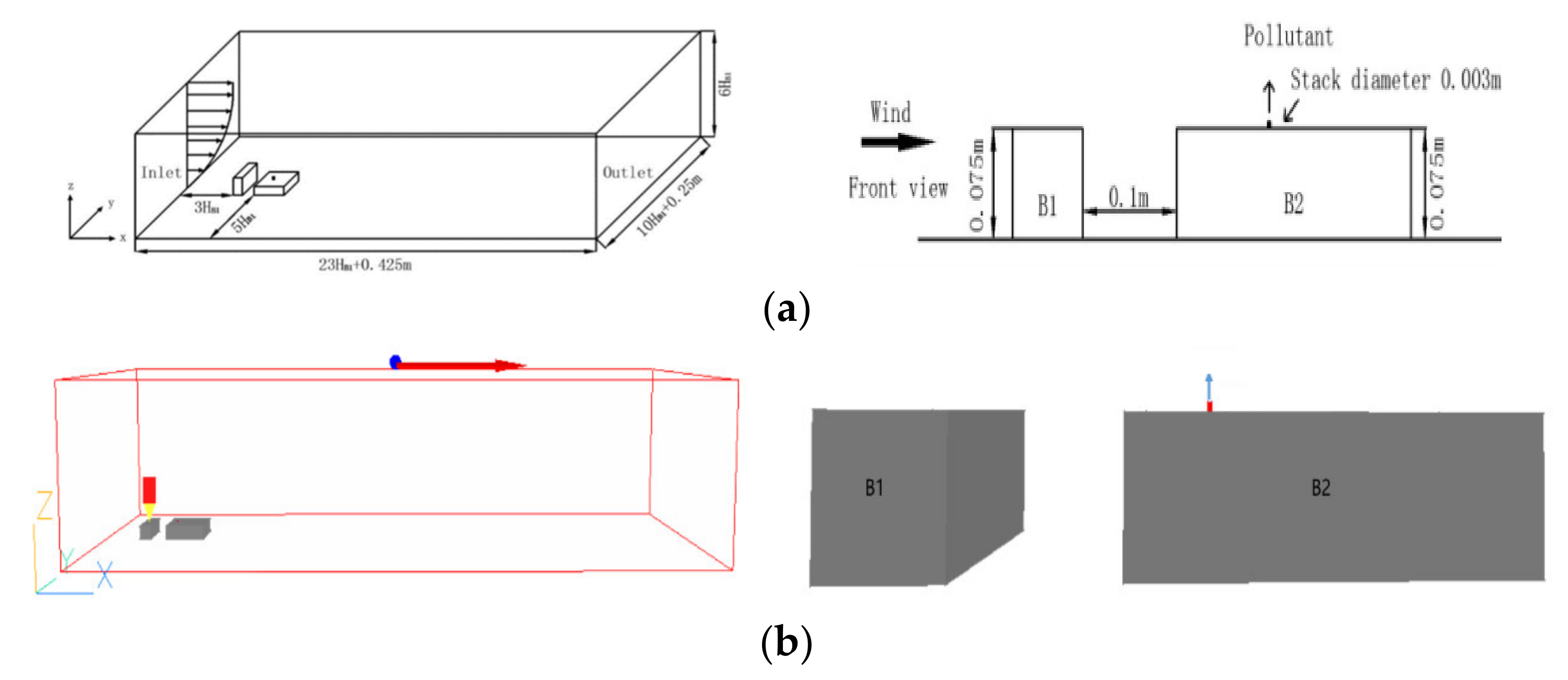
The results of the previous study, “Impacts of Upstream Building Height and Stack Location on Pollutant Dispersion from a Rooftop Stack” [24], were used as benchmark data. The physical model configurations are shown in Figure 2, which were based on the wind tunnel models established by Chavez et al. [25] in the wind tunnel experiments, at the Boundary Layer Wind Tunnel of Concordia University.

The wind flew from the left side (west wind); the average speed was described as following power law profile:

$$U\left(z\right)=6.2{\left(\frac{z}{0.075}\right)}^{0.31}\mathrm{m}/\mathrm{s}$$

(2)

where $U\left(z\right)$ is the average wind speed at the height of z above the ground.

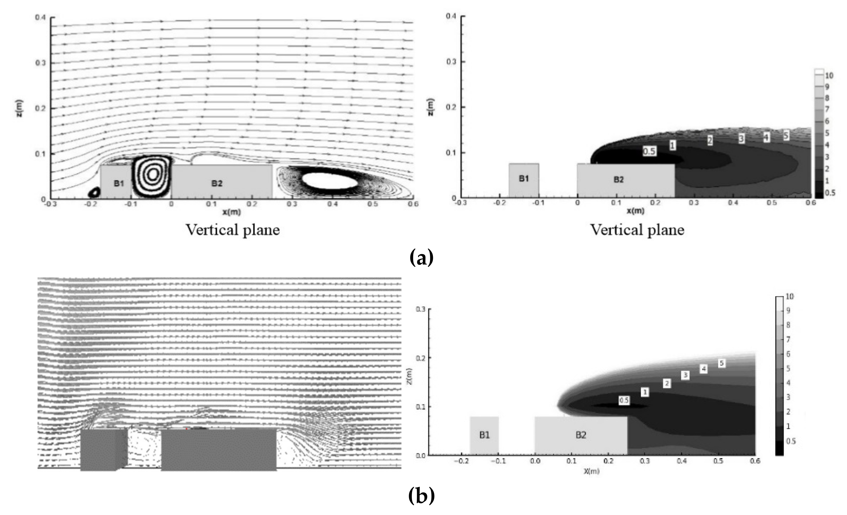
There were many cases in the reference paper, so the result of one case was selected to compare the result of the numerical simulations by CFD code PHOENICS version 6.0, using the standard k-ε turbulence model and governing equations mentioned in Section 2.3. The dimensions of the upstream building (B1) were 0.075 (length) × 0.25 (width) × 0.075 (height) m³, and the dimension of the downstream building (B2) were 0.25 (length) × 0.25 (width) × 0.075 (height) m³. The distance from the stack to the upwind edge of building B2 was 0.005 m, and the distance between two buildings was 0.1 m. The stack was 0.005 m high, and the stack diameter was 0.003 m. The pollutant SF₆ emitted from the stack was simulated as Q = 4.38 × 10⁻⁵ m³/s (Q was the flow rate of the pollutant at the outlet of the stack) and C_e (the concentration of SF₆ in the exhaust) was 10 ppm. Figure 3 qualitatively compares the flow field and normalized dilution contours between the reference paper and CFD simulation on the centerline plane of the buildings.

The study evaluated the dispersion of the plume by normalized dilution, as shown in following equation:

$$D_{\mathit{normalized}}=\frac{D_{r}Q}{U_{B2}{H}_{B2}^2}{ D}_r=\frac{C_e}{C_r}$$

(3)

where $D_{\mathit{normalized}}$ is the normalized dilution at a coordinate location, with C_r is the concentration of pollutant at the corresponding location. C_e = 10 ppm, Q = 4.38×10⁻⁵ m³/s, U_B2 = 6.2 m/s, and H_B2 = 0.075 m, so that $D_{\mathit{normalized}}$ = 1.256×10⁻⁸/C_r.

Figure 3a shows a tiny recirculation zone next to the upwind of B1. There was a clockwise vortex between B1 and B2, and a large wake vortex zone next to the downwind of B2. There were few pollutants in the region upwind of the stack. The pollutant concentration was in a high level on the roof of B2 downwind of the stack and in the wake vortex zone behind B2. Equation (3) shows that the pollutant concentration is inversely proportional to the normalized dilution. As the pollutant was conveyed downstream and mixed with the clean air, the degree of pollutant dilution increased, and the pollutant concentration decreased. Figure 3b presents the results simulated by CFD (PHONECIS version 6.0), which shows a reasonably good agreement with the results of the reference paper. Therefore, the results simulated by CFD code PHOENICS version 6.0 are accepted with the appropriate level of accuracy to demonstrate the numerical value reality. The turbulence model and solution techniques were used to investigate the plume behavior of the exhaust emitted from multiple stacks on the container ship.

4. Results

The results of the numerical simulation by CFD code PHOENICS version 6.0 were quantified analyzed to clarified the difference in C1_max, C1_1km and the plume heights between multiple stack emissions and single stack emissions. For the plume rise mainly occurring within 1 km of the stacks, and the maximum of C1 can be used to observe the maximum impact of ship pollution on the environment.

4.1. BL1 Simulations

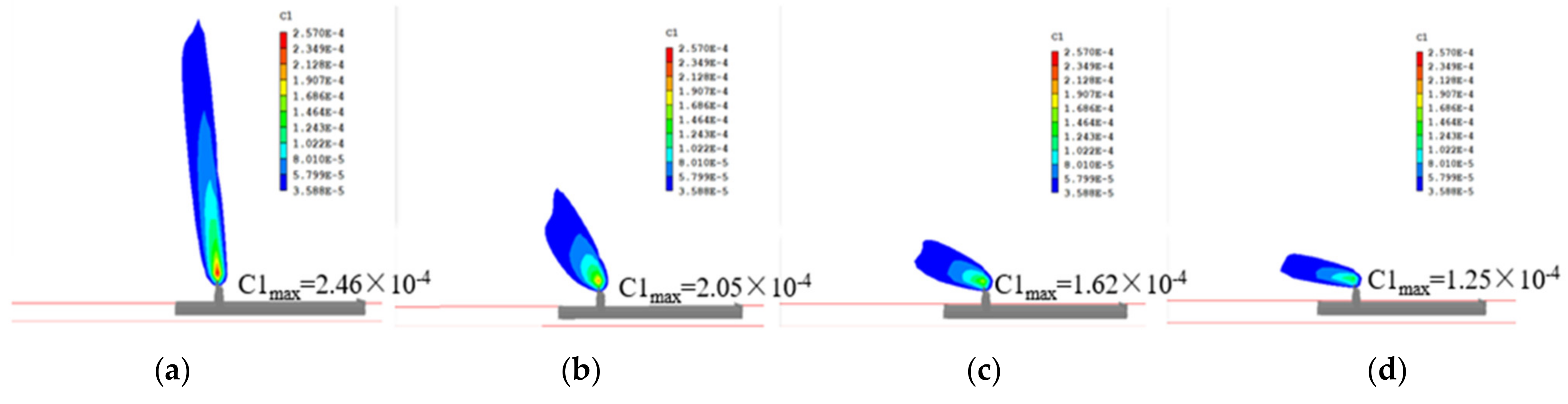
Figure 4 presents C1 (mass fraction of SO₂ in the plume) contours at different wind speeds. The C1_max-M1 was 16.5%, 13.8%, 10.9%, and 8.4% of C1₀-M1, respectively, when the V _wind was 1.5, 5, 10, and 15 m/s. The C1_1km-M1 was 0.47%, 0.56%, and 0.59% of C1₀-M1, respectively, when the V _wind was 5, 10, and 15 m/s. When the wind speed was 1.5 m/s, the location of C1_1km-M1 was outside the computational domain, so C1_1km-M1 were shown at wind speeds of 5, 10, and 15 m/s. The results show that as the wind speed increase, C1_max-M1 decrease and C1_1km-M1 increase. This indicates that with the increase of wind speed, the pollutant diffusion is faster and the plume conveying is more efficient.

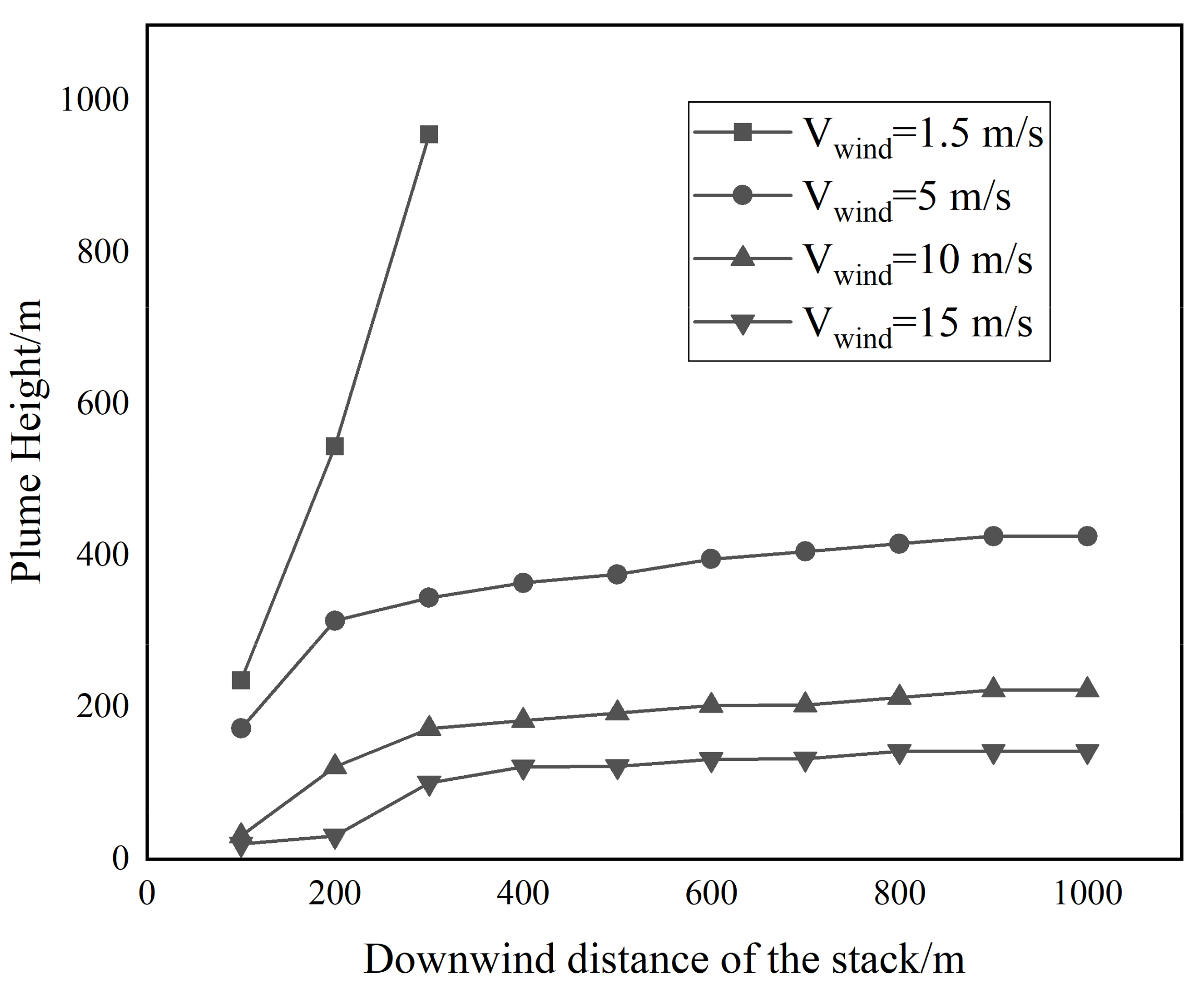
Figure 5 shows different plume heights at different wind speeds on the M1 plane. The plume had risen vertically to a great height before bending, and the plume height was beyond the computational domain at the point around 300 m downwind of the stack, when the wind speed was 1.5 m/s. As the wind speed increased, the plume rise tended to be diminished and further. At the point 1 km downwind of the stack, the plume height was approximately 142 m when the wind speed was 15 m/s. When the wind speed was 10 and 5 m/s, the plume heights at the point 1 km downwind of the stack was approximately 1.57 times and 2.99 times of that when the wind speed was 15 m/s, respectively.

4.2. BL2 Simulations

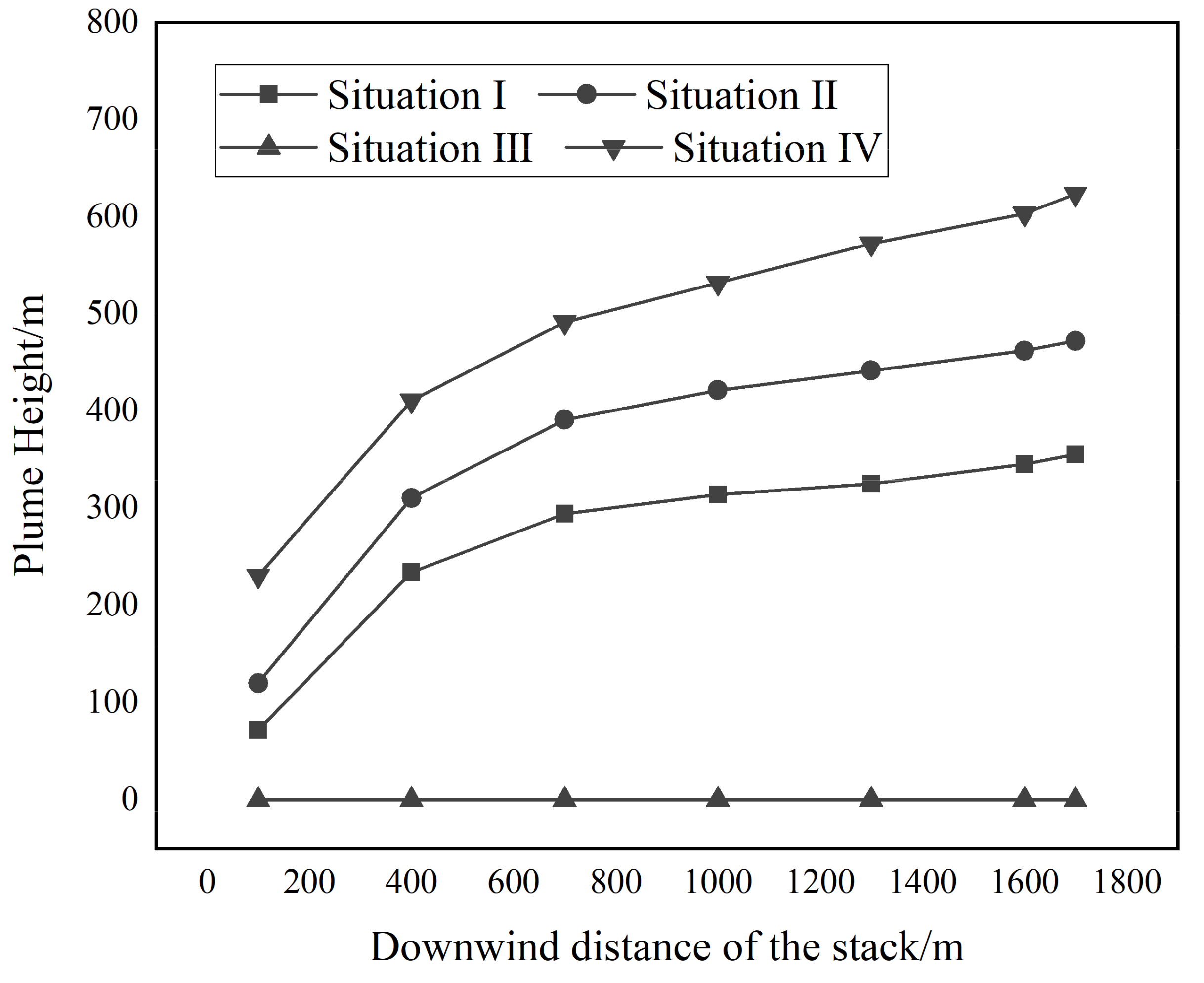
A switching approach was adopted in the simulations for stack configuration BL2, when the wind speed was 5 m/s. The approach was to divide the simulations into several situations, so that the exhaust emitted from different number of stacks, analyzing the difference in plume behavior between these situations. The situations included exhaust emitted from single main stack (Situation Ⅰ), exhaust emitted from single auxiliary stack (Situation Ⅱ), exhaust emitted from multiple auxiliary stacks (Situation Ⅲ), and exhaust emitted from single main stack with multiple auxiliary stacks (Situation Ⅳ).

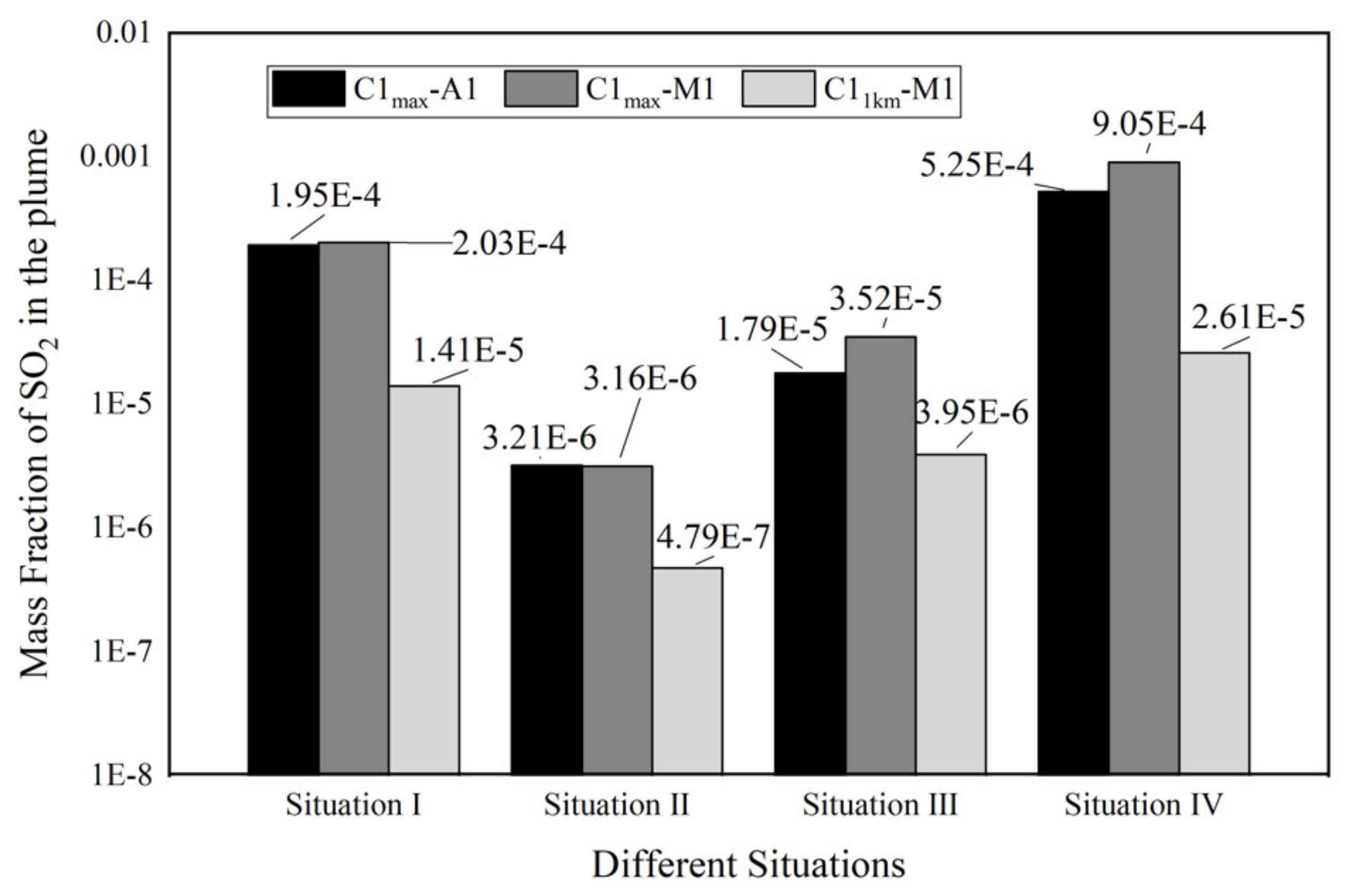
Figure 6 shows the results of C1_max-M1, C1_max-A1, and C1_1km-M1 in different situations. There was a significant difference in C1 between multiple stack emissions and single stack emissions. Compared to Situation Ⅰ, the C1_max-M1 in Situation Ⅳ was much higher. The C1_max-M1 in Situation Ⅲ was much higher than in Situation Ⅱ.

The results in Figure 6 show a significant difference in C1 between different situations. The C1_max-M1 was 3.52 × 10⁻⁵ when the exhaust emitted from multiple auxiliary stacks at the same time (Situation Ⅲ), which was approximately 186% of the sum of C1_max-M1 when exhaust was emitted from six auxiliary stacks individually (6 × 3.16 × 10⁻⁶). This meant that the C1_max-M1 in Situation Ⅲ was 86% higher than that in Situation Ⅰ, due to the multiple auxiliary stack emissions, as shown in

Table 4. BL2 simulations: The increase of C1 due to the multi-stack emissions in different situations.

C1 in Different Situations	C1max-M1 in Situation Ⅲ	C1max-M1 in Situation Ⅳ	C1max-A1 in Situation Ⅳ	C11km-M1 in Situation Ⅲ	C11km-M1 in Situation Ⅳ
The increase of C1 due to the multiple stack emissions	86% 1	329% 2	160% 2	37% 1	58% 2

¹ $\left[\frac{C1 \mathit{in} \mathit{Situation} \mathit{III}}{6\times C1 \mathit{in} \mathit{Situation} \mathit{II}}-1\right]$×100%; ²$\left[\frac{C1 \mathit{in} \mathit{Situation} \mathit{IV}-C1 \mathit{in} \mathit{Situation} \mathit{III}}{C1 \mathit{in} \mathit{Situation} \mathit{I}}-1\right]$×100%.

. The C1_max-M1 was 9.05×10⁻⁴ when exhaust emitted from all stacks at the same time (Situation Ⅳ), which was approximately 446% of that when exhaust emitted from single main stack (Situation Ⅰ). The C1_max-M1 in Situation Ⅲ was approximately 17.4% of that in Situation Ⅰ. Therefore, the C1_max-M1 in Situation Ⅳ was approximately 329% higher than that in Situation Ⅰ, due to all stack emissions, as shown in Table 4, and the C1_max-A1 in Situation Ⅳ was approximately 160% higher than that in Situation Ⅰ, due to all stack emissions. The increase in C1_max-A1 (160%), due to all stack emissions, was lower than that in C1_max-M1 (329%).

The results show that the influence of multiple stack emissions on C1 is significant because of the close distance between multiple stacks. The multiple stack emissions cause heat to accumulate near the stacks, slowing plume diffusion and increasing pollutant concentrations. The C1_max in the exhaust of multiple stack emissions is significantly higher than that of single stack emissions. This difference in C1 between multiple stack emissions and single stack emissions is decreased as the crosswind distance of the stack increases.

At around 1 km downwind of the main stack, C1_1km-M1 in Situation Ⅲ (3.95 × 10⁻⁶) was approximately 37% higher than the sum of C1_1km-M1 when exhaust was emitted from six auxiliary stacks individually (6 × 4.79 × 10⁻⁷). The increase of C1_1km-M1 (37%), due to the multiple auxiliary stack emissions, was lower than that of C1_max-M1 (86%). The increase of C1_1km-M1 (58%) due to all stack emissions (Situation Ⅳ) was lower than that of C1_max-M1(329%), as shown in Table 4. Therefore, the difference in C1 between multiple stack emissions and single stack emissions decreases as the downwind distance of the stack increases.

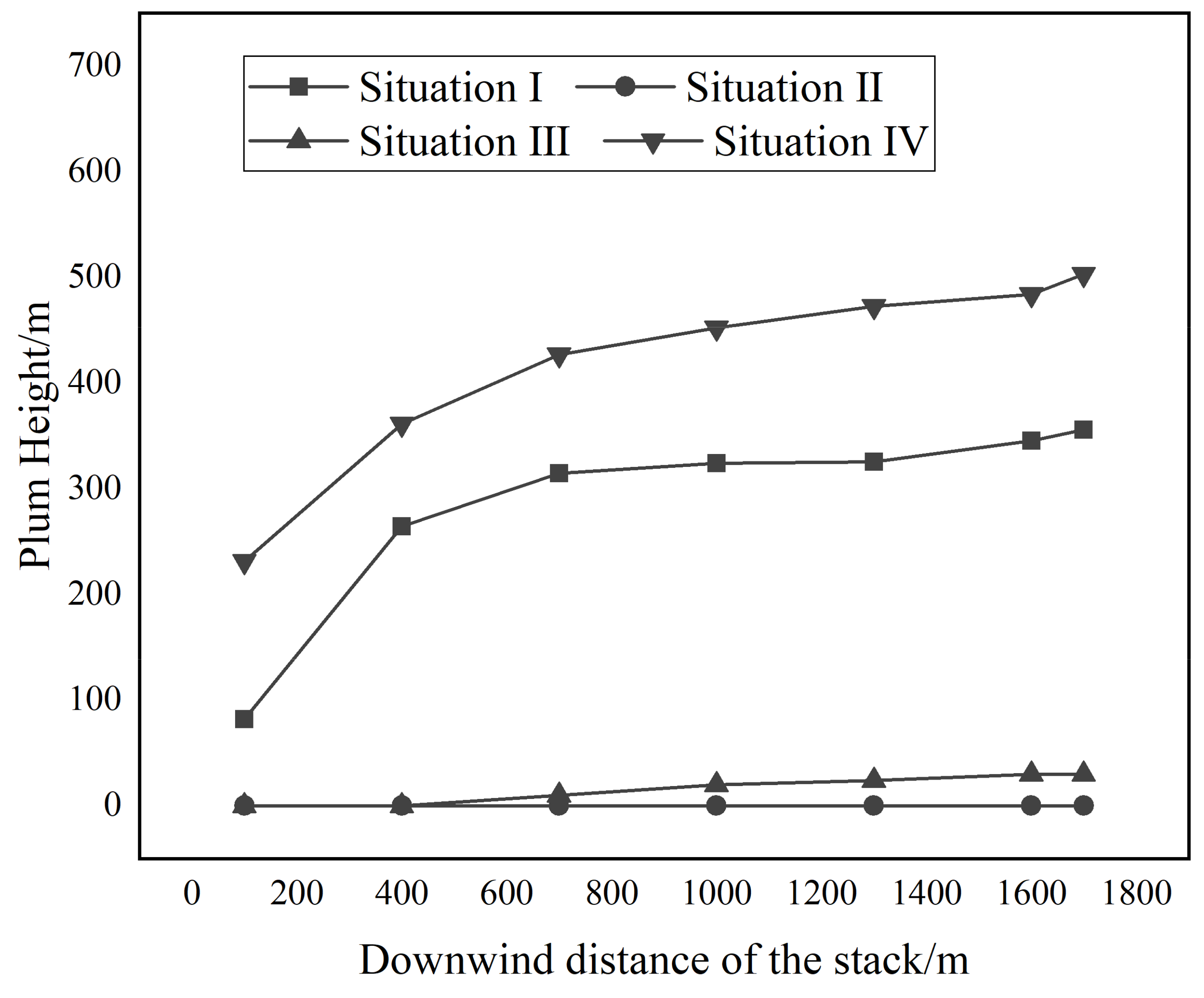
Figure 7 shows the plume height on the M1 plane when the wind speed was 5 m/s in different situations. The exhaust flow rate of the auxiliary stack was small, leading the plume rise to stop quickly in Situation Ⅱ. The line representing the plume height in Situation Ⅱ in Figure 7 is close to the X-axis. The plume height in Situation Ⅲ was approximately 30 m at the edge of the domain, which was higher than that in Situation Ⅱ. The plume in Situation Ⅰ and Situation Ⅳ kept rising within the calculation domain. The plume height in Situation Ⅰ was approximately 355 m at the edge of the domain. The plume height in Situation Ⅳ was approximately 500 m at the edge of the domain, which was 41% higher than that in Situation Ⅰ. The difference in the plume height between Situation Ⅳ and Situation Ⅰ was not kept at a fixed value in the calculation domain, and the maximum value reached approximately 100 m (the plume height in Situation Ⅳ was 182% higher than that in Situation Ⅰ), while the minimum value was approximately 400 m (the plume height in Situation Ⅳ was 37% higher than that in Situation Ⅰ).

4.3. BL3 Simulations

The results shown in BL2 simulations demonstrate that C1 and plume heights of multiple stack emissions were higher than those of single stack emissions. The BL3 simulations included another four situations to verify the results in Section 4.2: exhaust emitted from single main stack (Situation Ⅰ), exhaust emitted from two main stacks (Situation Ⅱ), exhaust emitted from multiple auxiliary stacks (Situation Ⅲ), and exhaust emitted from two main stacks with multiple auxiliary stacks (Situation Ⅳ).

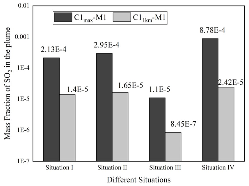
Figure 8 shows the C1_max-M1 and C1_1km-M1 in different situations when the wind speed was 5 m/s. The C1_max-M1 in Situation Ⅱ was higher than that in Situation Ⅰ, due to the two main stack emissions. The C1_max-M1 in Situation Ⅳ was higher than that in Situation Ⅰ, due to all stack emissions. The C1_max-M1 in Situation Ⅲ was lower than that in Situation Ⅰ, due to the small exhaust flow rate of the auxiliary stack, and the C1_1km-M1 in these four situations were lower than C1_max-M1, due to the diffusion of pollutants.

The differences in C1_max-M1 and C1_1km-M1 between multiple stack emissions and single stack emissions were quantified and analyzed, as shown in

Table 5. BL3 simulations: The increase of C1 due to the multi-stack emissions in different situations.

C1 in Different Situations	C1max-M1 in Situation Ⅱ	C1max-M1 in Situation Ⅳ	C11km-M1 in Situation Ⅱ	C11km-M1 in Situation Ⅳ
The increase of C1 due to the multiple stack emissions	39% 1	269% 2	18% 1	50% 2

¹ $\left[\frac{C1 \mathit{in} \mathit{Situation} \mathit{II}}{C1 \mathit{in} \mathit{Situation} \mathit{I}}-1\right]$×100%; ²$\left[\frac{C1 \mathit{in} \mathit{Situation} \mathit{IV}-C1 \mathit{in} \mathit{Situation} \mathit{II}-C1 \mathit{in} \mathit{Situation} \mathit{III}}{C1 \mathit{in} \mathit{Situation} \mathit{I}}\right]$×100%.

. The C1_max-M1 in Situation Ⅳ was 269% higher than that in Situation Ⅰ, due to all stack emissions, which was lower than the increase value in C1_max-M1 in BL2 simulations mentioned in Section 4.2 (329%). Therefore, the distance between stacks is a very important element for the change of C1_max-M1. The distance between two main stacks of configuration BL3 was 9.5 m, and the distance between the main stack and multiple auxiliary stacks of configuration BL2was 1.75 m. When multiple stacks with small exhaust flow rates are close to each other, the increase in C1_max-M1 due to multiple stack emissions is higher than that when multiple stacks with large exhaust flow rate are far away from each other. Further, Table 5 also shows that the difference in C1 is decreased as the crosswind and downwind distance of the stack increases between multiple stack emissions and single stack emissions. The result is consistent with that in BL2 simulations, mentioned in Section 4.2.

Figure 9 shows the plume heights on the M1 plane in different situations at a wind speed of 5 m/s. The exhaust flow rate of the auxiliary stack was small, leading the plume rise to stop quickly in Situation Ⅲ. The line representing the plume height in Situation Ⅲ in Figure 9 is close to the X-axis. The plume in Situation Ⅱ kept rising within the calculation domain (1700 m downwind of the stack), and the plume height was consistently higher than that in Situation Ⅰ. At around 1700 m downwind of the stack, the difference in plume height between Situation Ⅱ and Situation Ⅰ reached the largest value in the domain, which was approximately 117 m (the plume height in Situation Ⅱ was 33% higher than that in Situation Ⅰ). In Situation Ⅳ, the plume kept rising within the calculation domain. The difference in height between the Situation Ⅰ and Situation Ⅳ gradually increased with the increase of downwind distance of the stack, which reached approximately 268 m (the plume height in Situation Ⅳ was 75% higher than that in Situation Ⅰ) at around 1700 m downwind of the stack. Therefore, the exhaust plume height of multiple stack emissions is much higher than that of single stack emissions. The result is consistent with that discussed in Section 4.2.

5. Conclusions and Discussion

In this study, three simplified typical configurations on multiple stacks of the container ship were established based on real ships. The cases were simulated by CFD code PHOENICS version 6.0. The differences in C1 and plume heights between multiple stack emissions and single stack emissions were then quantified analyzed. The results show that there is a significant difference in plume behavior between the single stack emissions and the multiple stack emissions, and the different value has some spatial variation.

The C1 in multiple stack emissions is much higher than that in the single stack emissions, because the accumulation heat slows down the diffusion of the pollutant. The difference in the C1 between multiple stack emissions and single stack emissions decreases as the downwind and crosswind distances of the stack increase. In BL2 and BL3 simulations, C1_max-M1 of all stack emissions was 329% and 269% higher than that of single main stack emissions, respectively, and C1_1km-M1 of all stack emissions was 58% and 50% higher than that of single main stack emissions, respectively.

The distance between stacks is an important element in determining the C1_max-M1 difference between all stack emissions and single stack emissions. The distance between the main stack and the auxiliary stack was 1.75 m in configuration BL2, smaller than that between two main stacks which was 7.5 m in configuration BL3. Compared with single stack emissions, the C1_max-M1 of all stack emissions increased approximately 329% and 269%, respectively, in BL2 and BL3 simulations.

The exhaust plume height in all stack emissions is much higher than that in single main stack emissions, and in BL2 and BL3 simulations, the difference in height between Situation Ⅳ and Situation Ⅰ reached the largest value of approximately 100 and 268 m (the plume height in Situation Ⅳ was 182% and 75% higher than that in Situation Ⅰ), respectively, at around 500 and 1700 m downwind of the stacks.

This paper shows the mass fraction of SO2 in the exhaust and plume heights of multiple stack emissions are much higher than those of single stacks emissions. This study provides theoretical and technical support for ship research at a regional scale. Further studies of ship pollution in port areas should consider the significant difference in plume behavior between multiple stack emissions and single stack emissions.

References

- Cheng, L.; Yuan, Z.; Fan, X. An AIS-based high resolution ship emission inventory and its uncertainty in Pearl River Delta region. China Sci. Total Environ. 2016, 573, 1–10. [Google Scholar]
- Chen, D.; Tian, X.; Lang, J. The impact of ship emissions on PM2.5 and the deposition of nitrogen and sulfur in Yangtze River Delta. China Sci. Total Environ. 2019, 649, 1609–1619. [Google Scholar] [CrossRef] [PubMed]
- Feng, J.; Zhang, Y.; Li, S. The influence of spatiality on shipping emissions, air quality and potential human exposure in Yangtze River Delta/Shanghai, China. Atmos. Chem. Phys. Discuss. 2019, 19, 6167–6183. [Google Scholar] [CrossRef] [Green Version]
- Lv, Z.; Liu, H.; Yu, Q. Impacts of shipping emissions on PM2.5 air pollution in China. Atmos. Chem. Phys. 2018. [Google Scholar] [CrossRef] [Green Version]
- Fu, M.; Liu, H.; Jin, X. National- to port-level inventories of shipping emissions in China. Environ. Res. Lett. 2017, 12, 114024. [Google Scholar] [CrossRef]
- Winther, M.; Christensen, J.; Plejdrup, M. Emission inventories for ships in the arctic based on satellite sampled AIS data. Atmos. Environ. 2014, 91, 1–14. [Google Scholar] [CrossRef]
- UNCTAD. Review of Maritime Transport 2015. In Executive Summary and Final Report UNCTAD/RMT/2015 by the UNCTAD Secretariat; United Nations Conference on Trade and Development: Geneva, Switzerland, 2015. [Google Scholar]
- Zhang, Y.; Yang, X.; Brown, R. Shipping emissions and their impacts on air quality in China. Sci. Total Environ. 2017, 581, 186–198. [Google Scholar] [CrossRef] [PubMed]
- Aksoyoglu, S.; Baltensperger, U.; Prevot, A. Contribution of ship emissions to the concentration and deposition of air pollutants in Europe. Atmos. Chem. Phys. 2016, 16, 1895–1906. [Google Scholar] [CrossRef] [Green Version]
- Becagli, S.; Anello, F.; Bommarito, C. Constraining the ship contribution to the aerosol of the central Mediterranean. Atmos. Chem. Phys. 2017, 17, 2067–2084. [Google Scholar] [CrossRef] [Green Version]
- Zhao, M.; Zhang, Y.; Ma, W. Characteristics and ship traffic source identification of air pollutants in China’s largest port. Atmos. Environ. 2013, 64, 277–286. [Google Scholar] [CrossRef]
- Chen, D.; Fu, X.; Guo, X. The impact of ship emissions on nitrogen and sulfur deposition in China. Sci. Total Environ. 2020, 708, 134636. [Google Scholar] [CrossRef] [PubMed]
- Liu, Z.; Lu, X.; Feng, J. Influence of ship emissions on urban air quality: A comprehensive study using highly time-resolved online measurements and numerical simulation in Shanghai. Environ. Sci. Technol. 2017, 51, 202–211. [Google Scholar] [CrossRef] [PubMed]
- Murena, F.; Mocerino, L.; Quaranta, F. Impact on air quality of cruise ship emissions in Naples, Italy. Atmos. Environ. 2018, 187, 70–83. [Google Scholar] [CrossRef]
- Karla, P.; Eleanor, S.; Bryan, M. Impact of cruise ship emissions in Victoria, BC, Canada. Atmos. Environ. 2011, 45, 824–833. [Google Scholar]
- Vijayakumar, R.; Seshadri, V.; Singh, S. A Wind Tunnel Study on the Interaction of Hot Numerical modeling of exhaust smoke dispersion for a generic frigate and comparisons with experiments from the Funnel with the Superstructure of a Naval Ship. In OCEANS 2008—MTS/IEEE Kobe Techno-Ocean; IEEE: Piscataway, NJ, USA, 2008. [Google Scholar]
- Kulkarni, P.; Singh, N.; Seshadri, V. Experimental Study of the Flow Field over Simplified Superstructure of a Ship. International Journal of Maritime Engineering. Int. J. Marit. Eng. 2005, 147, 19–42. [Google Scholar]
- Park, S.; Cha, H.; Seol, S. Numerical research on establishing optimum design criterion of ship’s funnel. In Proceedings of the ASME International Mechanical Engineering Congress and Exposition, Boston, MA, USA, 31 October–6 November 2008. [Google Scholar]
- Kulkarni, P.; Singh, N.; Seshadri, V. Flow Visualization Studies of Exhaust Smoke-Superstructure Interaction on Naval Ships. Naval Eng. J. 2005, 117, 41–56. [Google Scholar] [CrossRef]
- Schulman, L.; Scire, J. Buoyant Line and Point Source (BLP) Dispersion Model User’s Guide; Environmental Research and Technology Inc.: Concord, MA, USA, 1980; pp. 1–218. [Google Scholar]
- Sumner, D.; Price, S. Flow-pattern identification for two staggered circular cylinders in cross-flow. J. Fluid Mech. 2000, 411, 263–303. [Google Scholar] [CrossRef] [Green Version]
- Environmental Protecting Research Institute of the Central Research Institute of Building and Construction. Wind tunnel study on plume rise and diffusion of the elevated stacks of Baoshan Iron. In Annex V of Environmental Impact Assessment of Baoshan Iron; Central Research Institute of Building and Construction Co Ltd MCC Group: Beijing, China, 1981; Available online: www.sslibrary.com. [Google Scholar]
- Kulkarni, P.; Singh, N.; Seshadri, V. The Smoke Nuisance Problem on Ships—A Review. Int. J. Marit. Eng. 2005. [Google Scholar] [CrossRef]
- Huang, Y.; Song, Y.; Xu, X. Impacts of Upstream Building Height and Stack Location on Pollutant Dispersion from a Rooftop Stack. Aerosol Air Qual. Res. 2017, 17, 1837–1855. [Google Scholar] [CrossRef] [Green Version]
- Chavez, M.; Hajra, B.; Stathopoulous, T. Assessment of near-field pollutant dispersion: Effect of upstream buildings. J. Wind Eng. Ind. Aerodyn. 2012, 104, 509–515. [Google Scholar] [CrossRef]
Figure 1.
The ship model, the domain, and the grids in CFD: (a) model setting on the X–Z plane; (b) model setting on the Y–Z plane.
Figure 2.
Physical models of the reference paper and CFD: (a) models of the reference paper; (b) CFD models.
Figure 3.
Qualitative comparison of the results between the reference paper and CFD simulation; (a) results of the reference paper; (b) results of CFD.
Figure 4.
BL1 simulations: The contours of C1 (mass fraction of SO2 in the plume) on the M1 plane at different wind speeds: (a) V wind = 5 m/s; (b) V wind= 10 m/s; (c) V wind = 15 m/s; (d) V wind = 20 m/s.
Figure 5.
BL1 simulations: Different plume heights at different wind speeds.
Figure 6.
BL2 simulations: C1 on specified vertical planes in different situations (V wind = 5 m/s).
Figure 7.
BL2 simulations: Different plume heights in different situations.
Figure 8.
BL3 simulations: C1 on M1 plane in different situations (V wind = 5 m/s).
Figure 9.
BL3 Simulations: different exhaust plume heights in different situations.