Continuous Spatio-Temporal High-Resolution Estimates of SWE Across the Swiss Alps – A Statistical Two-Step Approach for High-Mountain Topography

1 Introduction

Knowledge of the spatio-temporal distribution of snow (snow depth (SD) and snow water equivalent (SWE)) during winter in high-mountain regions is essential to understand key processes of hydrology (e.g., Kobold and Sušelj, 2005), glaciology (e.g., Zhang, 2005; Fujita, 2008), climatology (e.g., Salzmann et al., 2014), climate-cryospheric interactions (e.g., Hock et al., 2017) and of the related applied fields, such as natural hazard studies (e.g., Wood et al., 2016) or water resource studies. SD and SWE can be measured in-situ or derived from precipitation observations, although the relationship between (solid) precipitation and ground snow cover is not straightforward. Accurate and continuous spatial and temporal measurements for both precipitation and snow, are challenging to obtain in high-mountain regions, due to the difficulty of accessing such areas and of technically maintaining the sensors, etc., which results in a general high spatial and temporal scarcity of such data, and in associated high uncertainties (e.g., Goodison et al., 1998; Tapiador et al., 2012).

SD and SWE measurements are obtained annually in-situ on many mountain glaciers during winter mass balance monitoring (e.g., GLAMOS, 2018). These measurements are often the only ones available in remote high-mountain regions, thus making them an important source of data. However, these data usually only provide measurements for single points once a year, that is, at the end of the accumulation period (e.g., Huss et al., 2015). SD and SWE measurements are obtained in-situ in non-glacierized areas for the purpose of long-term climate monitoring (e.g., Seiz et al., 2010), avalanche warning (e.g., Lehning et al., 1999) and/or hydrological run off prediction. Unlike the measurements conducted on glaciers, these measurements are taken more frequently in time (twice a month in Switzerland), albeit at lower altitudes (from 1,059m.a.s.l. to 2,626m.a.s.l. in the Swiss Alps (cf. Jonas et al., 2009; Marty, 2017)).

Continuous temporal observations of SWE obtained with a cosmic ray sensor (CRS) were recently evaluated with promising results (e.g., Howat et al., 2018; Gugerli et al., 2019). The CRS counts the number of fast neutrons per hour from the secondary cascades of cosmic rays, which are attenuated by the hydrogen atoms of the snowpack. The neutron counts need to be corrected for changes in air pressure and the incoming cosmic ray flux and are inversely proportional to the SWE (Gugerli et al., 2019). The sensor can be deployed above or below the snowpack but in both cases the SWE observations are known to be influenced by changes in soil moisture through snow melt (e.g., Kodama, 1980; Sigouin and Si, 2016). These influences are limited if the CRS is placed on an ice surface (Howat et al., 2018; Gugerli et al., 2019).

Precipitation networks obtain observations at a much higher spatio-temporal resolution than SD and SWE measurements. Different techniques, which are also applied in mountain regions, and include precipitation gauges and/or weather radar estimates, are available to measure and estimate precipitation amounts. Precipitation gauges provide temporally continuous single point measurements, but are known to be heavily affected by undercatch caused by wind (e.g., Goodison et al., 1998; Sugiura et al., 2003; Fortin et al., 2008; Rasmussen et al., 2012; Pollock et al., 2013; Wolff et al., 2013) and by evaporation losses (e.g., Goodison et al., 1998). Kochendorfer et al. (2017) concluded that an all-weather unshielded weighing precipitation gauge measure less than 50% of the total amount of solid precipitation when the wind speed is higher than 5ms. Weather radars provide continuous spatial and temporal real-time information on precipitation estimates, by converting the backscattered pulses of hydrometeors within the atmosphere. Ground echoes, caused by the presence of high mountains, and the errors generated by beam shielding, beam broadening with distance, wet radome attenuation and hardware instability, can reduce accuracy of radar estimates considerably (e.g., Joss and Waldvogel, 1990; Germann and Joss, 2004; Germann et al., 2006). Therefore, radar-derived precipitation estimates are often compared or combined with precipitation gauge observations (e.g., Gabella et al., 2000; Gabella, 2004; Sideris et al., 2014; Gabella et al., 2017). Dual-polarization information can help the conversion of radar reflectivity into rainfall estimates. However, it cannot resolve all the issues related to the quantitative assessment of solid precipitation, because a unique relationship between shape/orientation and snowflake size does not exist. Further information on the challenges related to the derivation of quantitative estimates of solid precipitation by radars is provided by Saltikoff et al. (2015).

The possibility of exploiting weather radar precipitation estimates to reproduce snow accumulation over different glaciers in the Swiss Alps has recently been studied by Gugerli et al. (2020). They compared SWE measurements, obtained on several Swiss glaciers, with cumulative solid precipitation amounts obtained from the CombiPrecip radar-gauge product (MeteoSwiss, 2018) over four winter seasons. The observed difference between the measured SWE and cumulative precipitation showed large variations for different glaciers and, on occasion, consistent differences during some winter seasons.

Numerical weather prediction (NWP) models are another source of continuous temporal and spatial precipitation estimates. Only a few studies have so far investigated the use of NWP models for solid precipitation estimates in regions characterized by complex topography (e.g., Egli et al., 2009; Ikeda et al., 2010; Schirmer and Jamieson, 2015; Gugerli et al., 2021).

Gugerli et al. (2021) presented a novel approach to assess the performance of three spatio-temporally highly resolved gridded precipitation products based on different data sources (gauge-based, remotely sensed, and re-analyzed) with temporally continuous SWE observations taken by CRS deployed on two alpine glaciers (Plaine Morte and Findel) in Switzerland. They found a large bias of all precipitation products at a monthly and seasonal resolution. Moreover, they stated that the performance of the precipitation products largely depends on in-situ wind direction during snowfall events.

In addition to the challenges associated with measuring precipitation and snow parameters in high-mountain regions, the total seasonal amount and the spatio-temporal evolution of SD and SWE are complicated by various interactions between the local topography, solar radiation and weather conditions, which lead to high spatial variability, particularly for SWE (e.g., Rohrer et al., 1994; Wastl and Zängl, 2008; Kerr et al., 2013; Grünewald et al., 2014; Mott et al., 2014). Snow is re-distributed, for instance, by avalanches (e.g., Kuhn, 1995; Mott et al., 2019), as well as by creeping and sloughing as a result of the interplay between topography and gravitation forces (e.g., Gruber, 2007; Bernhardt and Schulz, 2010; Grünewald et al., 2014). The annual course of solar radiation leads to an enhanced snow melt, which affects SD and SWE during winter, especially toward the end of the winter season (e.g., Cline et al., 1998; Pohl et al., 2006; Mott et al., 2011; DeBeer and Pomeroy, 2017). Among the most important variables that influence the deposition and the redistribution of snow is wind (e.g., Pomeroy and Gray, 1995; Trujillo et al., 2007; Lehning et al., 2008). Wind-driven processes dictate the spatial distribution of snow accumulation at various magnitudes and at different spatial scales (e.g., Mott et al., 2018). Moreover, they displace snow from exposed to sheltered areas on the ground (e.g., Gauer, 2001; Mott et al., 2010), and cause the advection of precipitation, which is enhanced for snowfall because of the lower fall speed of snowflakes than of rain drops (e.g., Colle, 2004). Dadic et al. (2010) compared modeled wind fields of the ARPS mesoscale atmospheric model with SD observations from high-resolution lidar digital elevation models from a glacierized alpine catchment area. Their results show high horizontal wind speeds along steep slopes and ridges, and low wind speeds over flat areas, where higher snow accumulations were found. Depending on the wind direction, they observed erosion and reduced wind deposition on the windward side of the mountain ridges, while downward winds led to increased deposition in the lee of the mountain ridges. In a recent study, Gerber et al. (2019) have investigated the near-surface pre-depositional precipitation processes that shape snow accumulation in COSMO-WRF large-eddy simulations. They concluded that a minimum horizontal grid of 50m is needed to represent preferential deposition and local orographic precipitation enhancement. Their study indicated that near-surface preferential deposition can contribute by as much as 10% to the overall snow deposition. Cloud-dynamical processes and the mean advection may enhance precipitation amounts by as much as 20%. However, no clear relationship between wind speed and advection distance was found.

Statistical models are often applied to reproduce the distribution of snow by combining topographical parameters with regression trees (e.g., Elder et al., 1998; Balk and Elder, 2000; Erxleben et al., 2002; Winstral et al., 2002; Anderton et al., 2004; Molotch and Bales, 2005; López-Moreno and Nogués-Bravo, 2006; Litaor et al., 2008) and with multiple linear regressions (e.g., Elder et al., 1998; Jost et al., 2007). The most frequently used parameters are: elevation, topographic position, aspect, slope, and forest density. The statistical models of the aforementioned studies were able to explain up to 90% of the considered snow cover and SWE variability (Grünewald et al., 2013). However, the quality, the scale and the density of data should be considered to evaluate these results accurately. The majority of the aforementioned studies were based on specific sites with manual SD measurements available for a relatively small number of samples. As a consequence, the generalization of these models to other areas could not be proven consistently.

A study based on a large number of data and sites was carried out by Grünewald et al. (2013). They applied multiple linear regressions (MLR) to model SD distributions obtained from laser scanning for several small and medium-sized catchment areas in different mountain regions throughout the world. They built a specific model for each catchment area, as well as a global model that combined all the data from all the investigated sites. Their models explain much of the SD variability, but only for spatially aggregated data at scales of some hundreds of meters (smoothing the large variability generated by drifting snow at small scales). The most frequently used parameters in their models are: elevation gradient, slope, an aspect-based parameter and a wind-sheltering parameter. However, the coefficients and the importance of the parameters in the MLRs differed from catchment to catchment. Their models allowed 30–91% of the variability observed over single catchments to be explained. Moreover, the global model was able to explain 23% of the spatial variability, which led to the conclusion that it is difficult to generalize the relationship between topography and snow distribution.

Motivated by the scarcity and uncertainty of spatio-temporal observations of precipitation, SD and SWE in high-mountain regions, this study introduces a novel two-step statistical approach with low computational costs to derive continuous spatio-temporal, alpine-wide SWE estimates based on data from multiple sources. The continuous spatial and temporal SWE estimates were obtained by combining solid precipitation estimates with high-resolution topographical parameters and meteorological variables, including wind speed and shortwave radiation. Firstly, we extrapolated SWE estimates at a high spatio-temporal resolution over glacierized areas with SWE data from temporally continuous CRS observations and winter mass balance measurements, and then, we run the model over non-glacierized areas in order to assess its limits of applications.

The study sites and data are described in Section 2. Section 3 introduces the model and the procedures applied to derive and select the model variables. The results are presented in Section 4, and this is followed by a comprehensive evaluation and discussion of the model in Section 5. The concluding remarks and perspectives are provided in Section 6.

2 Study Sites and Data

The study was conducted in the Swiss Alps, according to a multi-sources data approach (Figure 1). The study concentrated on the Plaine Morte and Findel glaciers, where hourly SWE observations were available from a CRS for between October 2016 and May 2020. SD and SWE measurements were also available for six additional glaciers and 44 non-glacierized sites in the Swiss Alps. The different data sources used in this study are described in more detail in the following sections.

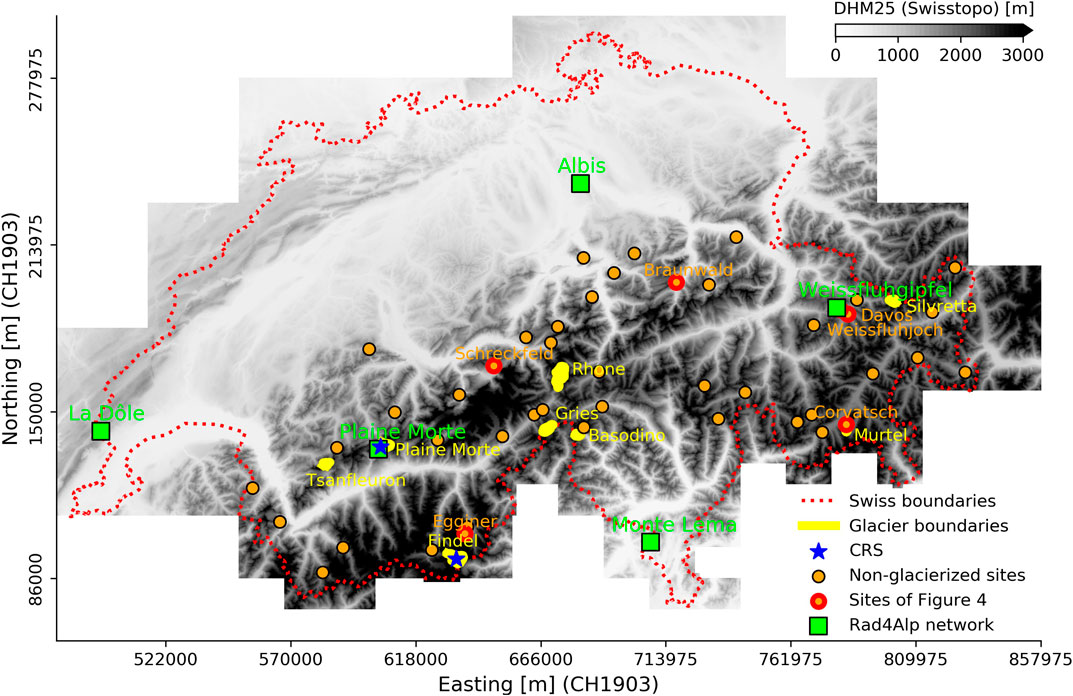
FIGURE 1. Distribution of the RAD4Alp weather radars, the CRSs, the considered glaciers with the end-of-season in-situ measurements and the non-glacierized sites with twice-monthly SWE measurements.

2.1 Snow Water Equivalent Measurements

2.1.1 Cosmic Ray Sensor Observations

In October 2016, a CRS was installed on the ice surface of the Plaine Morte glacier (46.38 N, 7.50 E, 2689 m.a.s.l.) in order to assess its performance regarding the daily SWE observations. In October 2018, another CRS was installed on the Findel glacier (46.00 N, 7.87 E, 3116 m. a.s.l.). These automated SWE observations were evaluated extensively against manual field measurements (snow pits, snow cores) between 2016 and 2019 (Gugerli et al., 2019; Gugerli et al., 2020). The CRS observations and 13 independent manual field measurements differ on average by a factor of 1.00 ± 0.10 (Gugerli et al., 2020). In our study, we used CRS observations from October 2016 to May 2020.

2.1.2 Manual In-Situ Measurements

The Swiss Glacier Monitoring Network (GLAMOS) observes more than 100 glaciers in the Swiss Alps (GLAMOS, 2018). SD and SWE are measured at single points, by means of snow probes and snow pits, in spring, when the snowpack reaches its maximum height (Huss et al., 2015; GLAMOS, 2018). In our study, we included measurements from eight Swiss glaciers (Rhone, Findel, Plaine Morte, Gries, Silvretta, Tsanfleuron, Basòdino and Murtèl), where the mean elevation (based on DHM25) of the eight glaciers varies between 2732 m. a.s.l (Plaine Morte) and 3237 m. a.s.l (Findel) (seeTable 1). The SD measurements are spatially distributed across the glaciers. SWE values are derived by including snow density information from snow pits or snow cores (GLAMOS, 2018). An overall uncertainty of about 5% is estimated for the bulk snow density estimation (cf. López-Moreno et al., 2020). The areal SWE is then determined by multiplying these mean density estimates with the spatially scattered SD measurements (Huss et al., 2015). In addition, since 2016 (2018), in-situ SWE measurements have also been obtained directly, during the winter season, at the CRS location on the Plaine Morte (Findel) glacier (Gugerli et al., 2019).

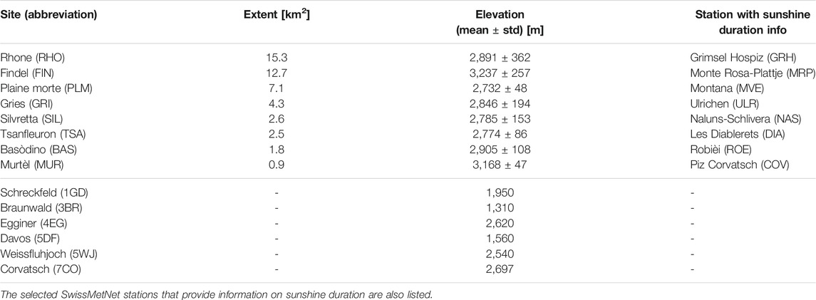
TABLE 1. Description of the glacier and non-glacierized sites.

2.1.3 Manual Measurements in Non-Glacierized Sites

Manual SWE measurements were also available from 44 non-glacierized sites, located at altitudes ranging from 1059 to 2626 m. a.s.l, and thus clearly at lower elevations than the measurements on the glacier sites. The measurements are made twice a month by the WSL Institute for Snow and Avalanche Research in Switzerland (SLF) (cf. Jonas et al., 2009; Marty, 2017). In our study, we used these data to test the model for non-glacierized areas and lower altitudes of the Swiss Alps. More detailed analyses are here provided for six of these sites (cf. Table 1), which represent different altitudes and regions in the Swiss Alps.

2.2 Precipitation Products

2.2.1 Weather Radar-Gauge Composites (CombiPrecip)

The CombiPrecip operational product (cf. MeteoSwiss, 2018) provides hourly precipitation sums over a 1 × 1 km² grid in the Swiss coordinate system. It combines real-time precipitation gauge measurements with radar estimates by co-kriging with an external drift (Sideris et al., 2014). The precipitation gauge measurements are processed before being used to generate the CombiPrecip product (e.g., Grüter et al., 2003). The quality of radar precipitation estimates decreases with the distance from the radar and is influenced by the Ear’s curvature, orographic partial beam shielding and the highly variable vertical reflectivity profile (MeteoSwiss, 2018). In general, the most reliable radar echoes originate in a surrounding distance of 3–60 km, and at altitudes at which mainly liquid hydrometeors occur (MeteoSwiss, 2018). Gugerli et al. (2020) evaluated the CombiPrecip product against end-of-season winter mass balance measurements from seven glaciers belonging to the GLAMOS network. In general, CombiPrecip showed lower estimates, ranging between a mean factor of 2.2 (Rhone) and 3.7 (Findel) over four winter seasons. The factor varies according to the winter season and the glacier. The largest underestimations of CombiPrecip were found on most glaciers in winter 2016/17, which was a particular dry winter all across Switzerland. However, a lower underestimation of CombiPrecip was found for Plaine Morte glacier, during the same winter.

2.2.2 Analysis of the Numerical Weather Prediction Model (COSMO-1)

Weusthoff et al. (2010) evaluated the ability of numerical weather prediction (NWP) models to represent precipitation observations of polarimetric C- band doppler radars. Their results show a better (or similar) performance of NWP models with increasing spatial resolutions, in particular for COSMO-7 (at a 7 km res.) compared with COSMO-2 (2 km res.). Egli et al. (2009), with reference to solid precipitation, included forecasted precipitation sums from COSMO-7 to estimate new daily SWE, and evaluated them against measurements from various devices located at the Weissfluhjoch site (Switzerland) at 2536 m a.s.l. Their results showed that COSMO-7 underestimated twice-monthly SWE measurements by 4%. Since 2016, the finer NWP model COSMO-1 has been operated by MeteoSwiss (MeteoSwiss, 2016) at a horizontal grid resolution of 1.1 km and highest model topography at 4268 m a.s.l. From the results of Weusthoff et al. (2010), it would appear that the highly resolved COSMO-1 model promises more accurate estimates of solid precipitation fields than the older models. In this study, we have used hourly precipitation and wind speed estimates (10 from the ground) from COSMO-1 analyses between October, 2016, and May, 2020. Station data, radiosondes, aircraft measurements and radar measurement fields are all assimilated in COSMO-1 analysis.

2.3 Additional Meteorological Data

2.3.1 Automatic Weather Station

An automatic weather station, which provides continuous measurements on shortwave radiation, is deployed at the CRS locations on the Plaine Morte and Findel glaciers. In this study, we also used information about sunshine duration (in minutes per hour) provided by MeteoSwiss automatic monitoring network stations (SwissMetNet). We selected the station closest to each glacier, considering the horizontal distance from each glacier and the difference in elevation. The list of the considered SwissMetNet stations is reported in Table 1.

2.3.2 Topographical Data

The topographical information used in this study (cf. Section 3) is based on a digital elevation model, with a resolution of 25 × 25 m² (DHM25), provided by Swisstopo (cf. Swisstopo, 2004).

3 Methods

The developed two-step statistical model, which allows spatio-temporal SWE estimates across the Swiss Alps to be derived, is presented hereafter. Step-1 was applied to obtain bias-corrected precipitation estimates (independent of the end-of-season in-situ SWE measurements) and to model the average hourly SWE variations (in the absence of precipitation). Step-2 was necessary to accurately increase the spatial resolution of the Step-1 estimates, using information from several glacier sites. The resulting two-step model combines data on precipitation, topography and wind speed (10 m above the ground) from multiple sources. Figure 2 schematically illustrates the two-step approach, which is briefly outlined hereafter, and described in more detail in Sections 3.1 and 3.2.

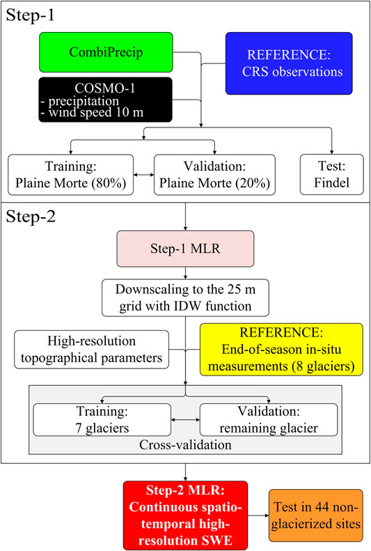
FIGURE 2. Flowchart showing the main assimilation, processing modeling and validation steps. The color of the boxes matches the color of the lines in the different plots in the paper.

3.1 Step-1: Adjustment of Precipitation Estimates to CRS Observations

The aim of Step-1 was to adjust (bias-correct) the precipitation data of CombiPrecip and COSMO-1 to the Plaine Morte glacier site by referring to the continuous temporal CRS data available there. Thus, the aim of the adjustment is to correct for the bias caused by precipitation undercatch and other systematic errors inherent in the single precipitation products, but also to account for other processes influencing the snow redistribution at the CRS location. For this purpose, we applied an MLR model (cf. Eq. 1) using the hourly SWE observation (CRS) as the response variable, and the precipitation and wind speed from CombiPrecip and COSMO-1 as the explanatory variables:

Where P_CPC,_i is the hourly precipitation of CombiPrecip, P_COSMO1,_i is the hourly precipitation of COSMO-1 and WS_COSMO1,_i is the hourly wind speed of COSMO-1.

The MLR was only trained with the CRS observations of the Plaine Morte glacier, and then tested with completely independent CRS observations from the Findel glacier. Table 2 reports the significance of the MLR variables and their coefficients to describe the hourly variations of SWE observed by the CRS on Plaine Morte. Since the variables are not standardized, their coefficients do not indicate their importance in explaining the CRS observations. Precipitation and wind speed are both positively correlated with the observed SWE variations (as indicated by the positive sign). The standard error (std err) shows the level of accuracy of the coefficients. From a statistical point of view, all the selected variables are highly significant, with a p-value <0.01 at a confidence interval of between 0.025 and 0.975. Step-1 MLR also involves a negative constant term, which models the average SWE variation in the absence of precipitation (according to the CRS observations). Therefore, in the case of dry conditions with no wind, the Step-1 model predicts a negative hourly SWE variation of 0.25 mm.

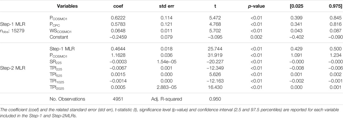
TABLE 2. Significance of the variables and models.

In order to better quantify the benefits provided by the Step-1 model, with respect to the precipitation products, we independently adjusted the precipitation estimates of CombiPrecip and COSMO-1. The adjustment coefficient was derived by minimizing the mean squared error with respect to the CRS observations on Plaine Morte (the same training data as those used in the Step-1 model). Thus, we obtained: Adjusted P_COSMO1 = 1.85 P_COSMO1 and Adjusted P_CPC = 2.28 P_CPC. The performance of the Step-1 model in representing the end-of-season in-situ SWE measurements distributed over the glacier sites (seeSection 4.1) was then compared with the performance of the adjusted CombiPrecip and adjusted COSMO-1 precipitation products.

3.2 Step-2: Downscaling With High-Resolution Topographical Parameters

In Step-2, the aim was to derive highly resolved spatial SWE estimates for the entire areas of the eight selected Swiss glaciers. For this purpose, we downscaled and further enhanced the Step-1 MLR model. We included topographical parameters and information on solar radiation (cf. Eq. 8), which allowed small-scale processes on the ground surface that influence the spatio-temporal SWE distribution to be taken into consideration. Therefore, the aim of the Step-2 model, was to model the processes of the following equation:

3.2.1 Downscaling

In order to produce smoother precipitation fields over the glaciers, we first downscaled the cumulative precipitation grids of Step-1 MLR from the 1 × 1 km² grid to the 25 × 25 m² grid of the DHM25 grid. We did this by resorting to an inverse distance weighting (IDW) function of the four nearest grid cells of the precipitation data. We then compared the generated 25 × 25 m² fields with the spatially scattered end-of-season in-situ snow accumulation measurements over eight glaciers. The observed differences were reduced by including the high-resolution topographical parameters in Step-2 MLR (minimizing the mean squared error between the Step-2 model and the in-situ measurements).

3.2.2 Topographical Parameters

The topographical parameters were derived from DHM25 and included the slope, aspect, topographic position index (TPI), East-West and North-South directional derivatives, maximum slope in the wind direction (Sx) and a solar radiation parameter (SR). TPI is defined as the difference in elevation between the central grid cell and the mean of the neighboring grid cells, and it allows terrain concavity (negative values) and convexity (positive values) to be represented. The Sx parameter was first introduced by Winstral et al. (2002) to model wind-redistributed snow. The relationship between Sx, TPI and wind error has already been investigated by Winstral et al. (2017) for COSMO-2 and COSMO-7 (which have a coarser spatial resolution than COSMO-1) and they observed a negative correlation between the mean wind speed and TPI. Here, we have computed each parameter with squared moving windows of various sizes, ranging from 75 × 75 to 2,025 × 2,025 m. A subset for Findel is reported in Figure 3. The SR parameter was obtained as a function of the derived slope, aspect and the relative Sun position for each hour of the day, and for each day of the year, neglecting atmospheric attenuation, and is described by the following equations:

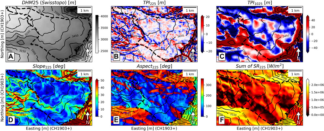
FIGURE 3. Example of the topographical parameters derived from DHM25 (A) for Findel glacier (glacier outline shown with the dashed line) including elevation contours (solid lines). The TPIs computed with a 225×225 m² and 1025×1025 m² moving window, respectively, are shown in (B,C). The slope and aspect computed with a 225×225 m² moving window are shown in (D,E) (F) presents the sum of the modeled solar radiation computed with a 225×225 m² moving window, for the 2019/20 winter season.

Where ASP is the aspect, SLP the slope, δ the solar declination, jjj the day of the year; In the solar irradiance at the top of the atmosphere, Isc the solar constant approximated to 1,361 W/m² (cf. Kopp and Lean, 2011); β the solar height, ϕ the latitude (46.4 for Switzerland), ω the hourly angle; ψ the solar azimuth; I₀ the solar intensity, which depends on the angle of incidence. We evaluated the quality of I₀ by comparing it with the shortwave radiation measurements of the AWS located on the Plaine Morte glacier (cf. Figure 4). We then improved our I₀ parameter with Eq. 8, by including information on sunshine duration (in minutes per hour), as obtained from the closest SwissMetNet station.

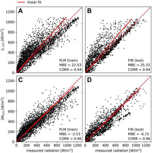
FIGURE 4. Scatterplot in which the modeled solar radiation (I₀, 225) and measured shortwave radiation, measured by the AWS located on Plaine Morte (A) and on Findel (B) are compared (C) compares the solar radiation adjusted with cloud cover information (SR₂₂₅) on Plaine Morte by minimizing the mean squared error of (A)(D) compares adjusted solar radiation with cloud cover information on Findel, using the correction factor obtained from Plaine Morte. The correlations (CORR) and mean bias errors (MBE) are reported on the graphs.

Where f is 0.33 and corresponds to the optimal value that minimizes the mean squared error of SR with respect to the shortwave radiation measured by the AWS on Plaine Morte and S_min,i is the sunshine duration, in minutes, measured during the specific hour. The sum of the modeled radiation received over the Findel glacier during the 2018–2019 winter is shown in Figure 3F, where the hourly estimates were validated at the CRS location (seeFigure 4). Findel is an independent test site and it is evident that this coefficient also improves the estimated shortwave radiation for Findel, as it increases the correlation from 0.94 to 0.96 and reduces the mean bias error from 25.32 to −6.72 mm. Without the sunshine duration information from the nearby station, the intensity of the received solar radiation would be overestimated in many cases. Figure 3F and Figure 3G show that south oriented slopes in general receive more shortwave incoming radiation. This most likely influences the total amount of snow present at the end of the winter season.

3.2.3 Feature Selection

In order to only include significant explanatory variables in the Step-2 MLR model, we applied a stepwise feature forward selection, which automatically includes, one by one, the variable that explains the most significant part of the variance of the response variable (in-situ SWE measurements). The selection stops when no more variables are able to explain a significant part of the variance. The selected variables are introduced in the following order: Step-1 MLR, COSMO-1 precipitation, modeled solar radiation based on aspect and slope derived with a 225 × 225 m² square moving window (SR₂₂₅), TPI for 225 × 225, 525 × 525, 1025 × 1025 and 2025 × 2025 m² moving windows (TPI₂₂₅, TPI₅₂₅, TPI₁₀₂₅ and TPI₂₀₂₅). Details of the significance and importance of the variables for Step-2 MLR to explain the end-of-season SWE are reported in Table 2. The intercept term in Step-2 MLR is set to 0, and the variables are not standardized. As all the variables are highly significant, and the confidence interval of their coefficients is relatively small, the robustness of MLR is enhanced. Step-2 MLR was tested using a “leave-one glacier-out” cross validation strategy, that is, the coefficients were determined for seven glaciers and the resulting regression model was compared with the end-of-season in-situ measurements of the remaining glacier.

The final equation of Step-2 MLR involved the use of Eq. 9, where the topographical parameters were multiplied by the number of hours of each specific winter season to facilitate the application of Step-2 MLR to smaller temporal scales. Equation 10 was used to produce MLR estimates at hourly timescales and the resulting time series were re-evaluated with CRS observations and field measurements over the Plaine Morte and the Findel glaciers.

In order to analyze the variance explained by the variables included in Step-2 MLR in more detail, we built a simple linear regression to correct the bias between the Step-1 MLR estimates and the end-of-season in-situ measurements of the eight glaciers (SLR = 0.97 Step-1 MLR). We then computed the difference between the in-situ measurements and SLR in order to calculate the residuals. The residuals are compared with TPI₂₂₅ in Figure 5A, and with the modeled radiation SR₂₂₅ in Figure 5B. Both figures show negative correlations, and the inclusion of TPI₂₂₅ and SR₂₂₅ in the Step-2 model should therefore allow the Step-1 MLR estimates to be improved. It is in particular possible to notice that the Step-1 MLR model underestimates in-situ measurements for negative TPIs (concavities) and overestimates them for areas affected by strong radiation.

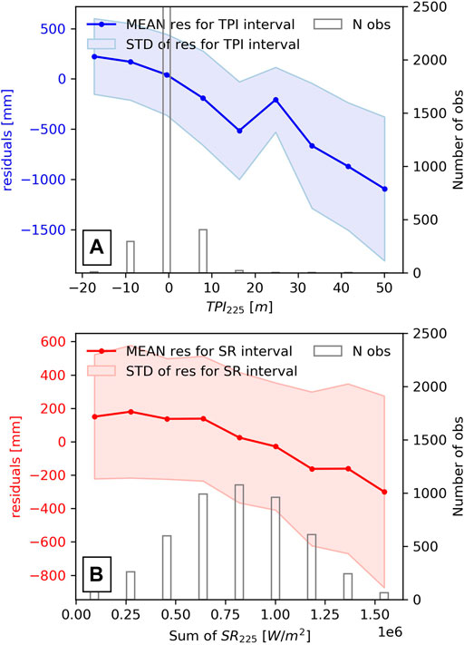
FIGURE 5. (A) shows the relationship between the residuals (SWE_{end-of-season}−SWE_{0.97 Step-1}) and TPI₂₂₅, while (B) describes the relationship between the residuals and sum of SR₂₂₅ for the entire winter seasons. All the measurements of all the glaciers and winter seasons are considered. The bars indicate the number of ground measurements related to the specific interval of the TPI₂₂₅ (and the SR₂₂₅) values.

3.3 Performance Assessment

We computed the ratio shown in Eq. 11 to evaluate the glacier-wide cumulative estimates of the precipitation products (over the winter season) and the Step-1 and Step-2 MLR models against the end-of-season in-situ SWE measurements (cf. Section 4.1). The ratio was weighted with the number of in-situ measurements performed within the 1 × 1 km² grid of the CombiPrecip, COSMO-1 and Step-1 MLR or the 25 × 25 m² grid of Step-2 MLR.

Where P_i corresponds to the precipitation or model estimate in a single m grid cell, and ni to the number of in-situ measurements in the same m grid cell.

4 Results

The intermediate and final results of the Step-1 and Step-2 MLR models used over the considered glaciers are presented hereafter. The performance is assessed by evaluating the results against independent spatially scattered end-of-season in-situ SWE measurements (Section 4.1) and temporally continuous CRS observations (Section 4.2). An evaluation of non-glacierized sites in the Swiss Alps is also presented (Section 4.3) using the independent twice-monthly manual SWE measurements.

4.1 Spatial Distribution of the Cumulative Precipitations and Total SWE

Figure 6 shows the resulting cumulative precipitation and total SWE between October 2018 and April 2019 for the Findel glacier. The results of all the other glaciers considered in our study are reported in the Supplementary Material Section S1. Figures 6A–C provide (intermediate) results on the precipitation estimates for the adjusted CombiPrecip product, the adjusted COSMO-1 model and the Step-1 MLR model, and 6D shows the (final) Step-2 MLR model. Figure 6A shows a much larger spatial variability of the in-situ SWE estimates than of the adjusted CombiPrecip estimates, which is obviously due to the spatial resolution of the data. Moreover, the minima of the adjusted CombiPrecip is clearly located at a higher altitude (south-east), and thus exactly where the largest SWE amounts are found for the in-situ measurements. A similar spatial variability pattern can be observed for the comparison against COSMO-1 (Figure 6B), where a much larger spatial variability is again observed for the in-situ measurements. However, COSMO-1 agrees better with the in-situ measurements than CombiPrecip. Looking at the results of Step-1 MLR (Figure 6C), it is possible to see a larger spatial variability, with smaller estimates at lower altitudes and larger estimates at higher altitudes. This effect is a result of considering the wind speed in the model. In fact, COSMO-1 wind speeds usually become stronger over Findel as the altitudes increase. Finally, the local variability improves with the inclusion of high-resolution topographical parameters in Step-2 MLR (Figure 6D), as indicated by the higher correlation with the in-situ SWE measurements (0.73 compared to 0.66). Moreover, local SWE maxima are estimated where the TPI₂₂₅ is negative.

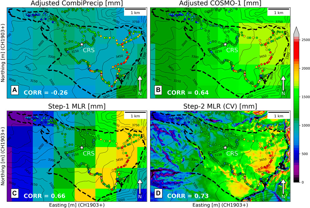
FIGURE 6. Cumulative precipitation maps (colored grid cells) and in-situ measurements (colored dots) over the Findel glacier at the end of the 2018/19 winter season (24.10.18–17.04.19). The glacier outline is shown with the dashed line and elevation contours are shown with solid lines (A,B) show precipitation estimates of adjusted CombiPrecip and adjusted COSMO-1 (C,D) show the model outputs of Step-1 MLR and Step-2 MLR.

The good overall performance of Step-1 MLR is confirmed in Figure 7, which shows the ratios between the cumulative precipitation and the end-of-season in-situ SWE for each winter season and each glacier (cf. Eq. 11). The ratios between Step-1 MLR and in-situ SWE are close to 1 for all the glaciers, and this pattern remains consistent for the Step-2 MLR results. In general, an increase in the ratios can be observed from the 2016/2017 winter to the 2019/2020 one, especially for CombiPrecip. However, when analyzing the CombiPrecip ratio over the different winter seasons, it is important to note that only three radars (Monte Lema, Albis and La Dôle) were operational in 2012. The Rad4Alp network was extended in 2014 with the addition of a weather radar station on the Pointe de la Plaine Morte, and in 2016 with a radar at Weissfluh. However, since COSMO-1 data have only been available to us from 2016, the Step-2 model only covers the years since then.

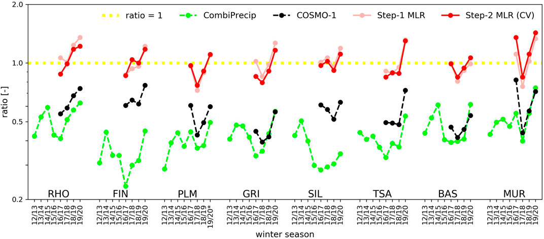
FIGURE 7. Ratio of the cumulative precipitation of the precipitation products to the SWEs, as estimated with the different models, and the end-of-season glacier-wide winter mass balance. *The 19/20 ratio for the Plaine Morte glacier was derived considering the CRS observations as no manual measurement were conducted in this winter season.

The scatterplots in Figure 8 compare the cumulative precipitation with in-situ SWE measurements of the four winter seasons and the eight glaciers. Figure 8B shows in-situ SWE measurements compared with the adjusted CombiPrecip and adjusted COSMO-1 precipitation (Figure 8C). A significant higher correlation may be noted for the adjusted COSMO-1 estimates (0.67) than for the adjusted CombiPrecip ones (0.48). Figures 8E,F show the correlation for Step-1 MLR (0.74) and Step-2 MLR (0.78). The comparison of the Findel glacier is highlighted with colored dots. The correlation of CombiPrecip with the in-situ SWE measurements is negative for all the investigated winter seasons, while it is positive for the adjusted COSMO-1 precipitation estimates. Step-1 MLR and Step-2 MLR both show an improvement. However, the higher spatial resolution of Step-2 further improves the continuity of the SWE estimates over the glacier sites. The good performance of Step-2 MLR indicates the power of the model to take into account the specific topographical characteristics of each glacier site and thus to improve confidence in distributed modeling across the Alps. The boxplots shown in Figure 8A indicate the distribution of all in-situ measurements (of the eight glaciers) and the distribution of the in-situ measurements for individual years of the Findel glacier. Figure 8D shows the distribution of CombiPrecip and COSMO-1 estimates and Figure 8G the distribution of Step-1 and Step-2 MLRs estimates. Observing the interquartile ranges, it is clear that for individual years, the spatial variability over the glacier area of Step-1 MLR and Step-2 MLR is much larger than the spatial variability of CombiPrecip and COSMO-1 and is closer to the spatial variability of the in-situ measurements. Finally, Table 4 reports the performance of both models and all the precipitation products, for each glacier and each winter season. In general, Step-2 MLR achieves higher correlation values, except for Plaine Morte and Gries. This is due, at Plaine Morte, to the very low spatial variability of SWE and, at Gries, to the small number of available in-situ measurements, in particular for the 2016/2017 and 2017/2018 seasons.

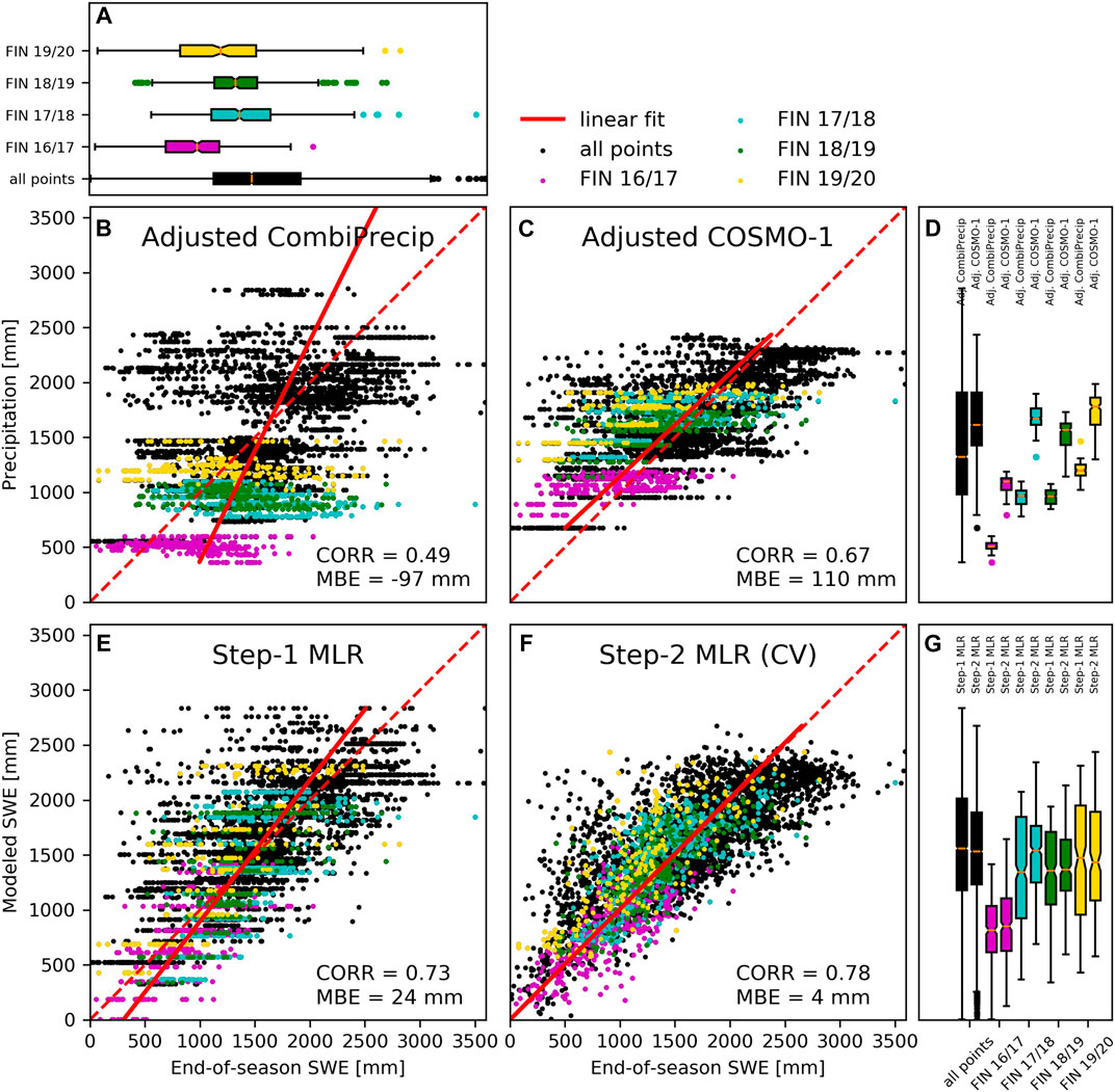
FIGURE 8. Scatterplots of the in-situ SWE measurements and cumulative precipitation and the total SWEs estimated by the different products and models for all the glaciers. The colored dots are related to the Findel glacier estimates and the different colors indicate different winter seasons (B): Adjusted CombiPrecip (C): Adjusted COSMO-1 (E): Step-1 (F): Step-2 cross validation. The correlations (CORR) and mean bias errors (MBE) with all in-situ measurements are reported on the graphs. The boxplots shown in (A) represent the distribution of all in-situ measurements (of the eight glaciers) and the distribution of the in-situ measurements for individual years of the Findel glacier (D) shows the distribution of CombiPrecip and COSMO-1 estimates and (G) shows the distribution of Step-1 and Step-2MLRs estimates.

4.2 Temporal Evolution of the Modeled SWE

Figure 9 shows the temporal evolution of the modeled SWE for Step-1 and Step-2 MLR compared with CRS observations and field measurements on Plaine Morte (2016–2020) and Findel (2018–2020), and the cumulative precipitation of CombiPrecip and COSMO-1. An overall quantitative assessment on the differences between CombiPrecip, COSMO-1 precipitation, Step-1 MLR, Step-2 MLR and CRS observations and manual measurements is also provided in Table 3, which reports the mean bias errors. The data used for the evaluation are completely independent of the training data for Findel and partly dependent for the Plaine Morte glacier, as Step-1 MLR was trained with CRS observations from Plaine Morte. Step-1 and Step-2 MLRs overestimate the two first manual measurements for Plaine Morte in December and January in the 2016/2017 season (Figure 9A), while the cumulative estimates agree well with the field measurements in March. The estimates of the models match well with the first SWE measured in the field at the beginning of the 2017/2018 winter season (Figure 9B), even though no CRS observation was available until December. The last field measurement of the season is significantly higher than the estimates of the MLRs and the observations of the CRS. The CRS observations and MLRs estimates agree much better with the field measurements for the 2018/2019 season (Figure 9C). Finally, during the 2019/2020 season (Figure 9D), the MLRs match very well with the field measurement made early on in the season, but are clearly higher at the end of the season, compared with the CRS observations.

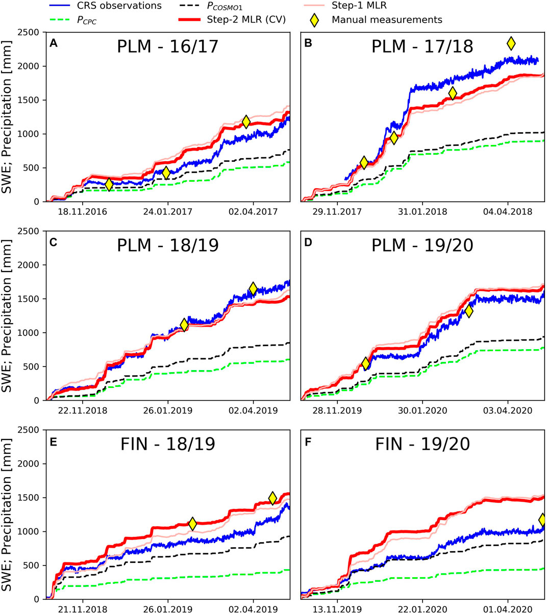
FIGURE 9. Time series of the Step-1 and Step-2 estimates, as obtained from the MLR models with SWE observations from the CRS, manual SWE measurements, CombiPrecip and COSMO-1 precipitation estimates (A): Plaine Morte 16/17 (B): Plaine Morte 17/18 (C): Plaine Morte 18/19 (D): Plaine Morte 19/20 (E): Findel 18/19 (F): Findel 19/20.

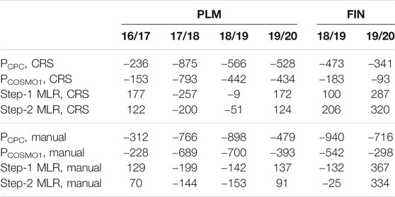
TABLE 3. CombiPrecip, COSMO-1 precipitation, Step-1 MLR and Step-2 MLR mean bias errors [mm] with respect to CRS observations and manual measurements performed during the winter seasons on the Plaine Morte and Findel glaciers.

Lower values can be observed for the CRS observations for Findel, which is a completely independent testing site for the models, than for the field measurements in the 2018/2019 winter (Figure 9E). However, the cumulative estimates of the MLR models, agree well with the manual SWE measurements. The Step-1 and Step-2 MLR models show higher values than CRS in the 2019/2020 season (Figure 9F), starting from December, because of the large amount of precipitation estimated by COSMO-1. In fact, the difference between the CRS observations and the COSMO-1 estimates is reduced to a great extent on Findel, compared with the Plaine Morte glacier.

4.3 SWE Estimates in Non-glacierized Sites

The glacier sites in our study, and glacier sites in general, show certain analogies regarding their mean altitude and the relative morphology of the terrain, which typically result in higher accumulations of precipitation than in the surrounding areas. In order to evaluate the possibility of applying Step-2 MLR to mountain ranges, the model was also compared with SWE measurements taken manually twice a month at non-glacierized sites in the Swiss Alps. Generally, these non-glacierized sites are located at lower elevations, which means they are also influenced more by snow melt.

Figure 10 compares the SWE measurements and the cumulative precipitation of CombiPrecip, COSMO-1, Step-1 and Step-2 MLRs. The overall correlations for CombiPrecip, COSMO-1, Step-1 MLR and Step-2 MLR are 0.60, 0.52, 0.45 and 0.53, respectively, while the mean bias errors are 22, 25, 8, and 31 mm. Melt can cause negative SWE variations, which cannot be represented by cumulative precipitation. Moreover, the MLR models were not trained to predict high negative SWE variations, because the snow melt is usually negligible during winter at glacier site altitudes. When the negative variations of the measured SWE are removed, the CombiPrecip, COSMO-1, Step1 MLR and Step-2 MLR correlation increase to 0.60, 0.65, 0.59, and 0.63, respectively, while the mean bias errors decrease to −5, −1, −16, and 12 mm. The poor performance of the Step-1 model indicates that it is not suitable for non-glacierized sites. A more detailed analysis is provided in Figure 11 for the six sites reported in Table 1. Here, the Step-1 and Step-2 estimates and cumulative precipitations are compared with the twice-monthly SWE measurements over the four winter seasons (see the Supplementary Material for the time series of the other stations). Step-1 MLR often results in lower values than thus of the manual measurements, while the Step-2 MLR estimates agree much more. Only for the Egginer station during the 2016/2017 season and partly in the 2017/2018 season, can we observe lower values. The COSMO-1 and CombiPrecip discrepancies, with respect to the manual measurements, are reduced, compared to the glacier sites in our study, and this often leads to generally higher values from the MLRs models than from manual measurements (e.g. the Weissflujoch, Figure 11E).

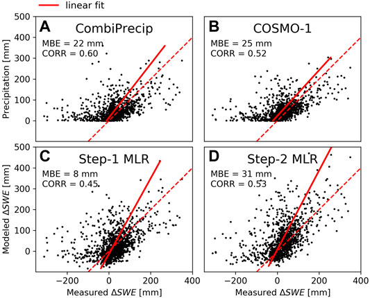
FIGURE 10. The twice-monthly SWE measurements on 44 non-glacierized sites and four winter seasons compared with (A): CombiPrecip (B): COSMO-1 (C): Step-1 MLR (D): Step-2 MLR.

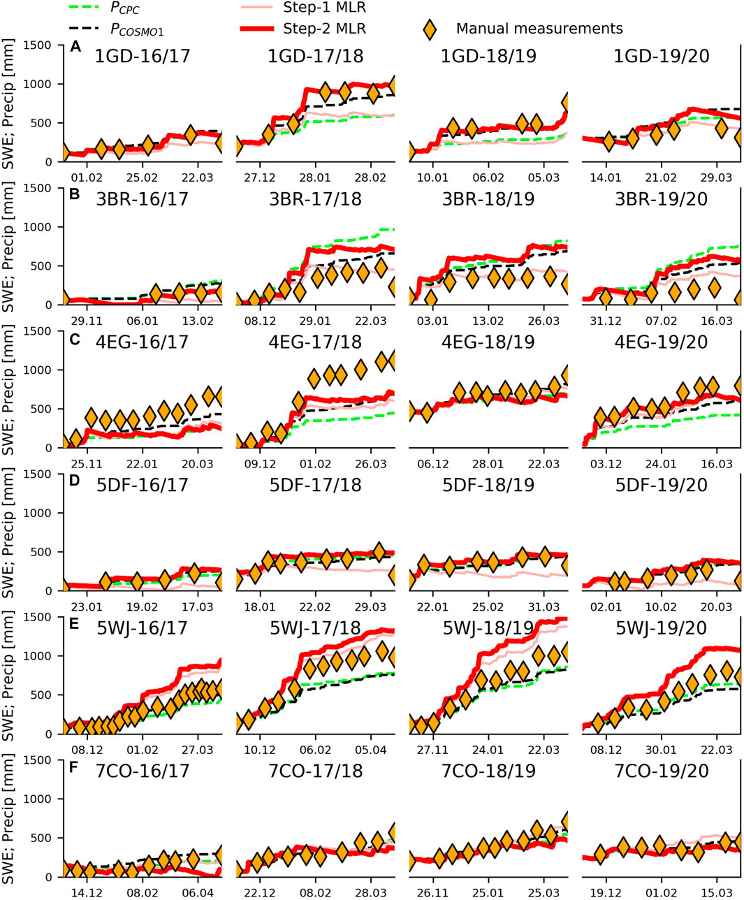
FIGURE 11. The twice-monthly SWE measurements of six stations compared with the cumulative precipitation and MLR estimates for the four winter seasons (A): Schreckfeld (elevation: 1,950 m) (B): Braunwald (1,310 m) (C): Egginer (2,620 m) (D): Davos (1,560 m) (E): Weissfluhjoch (2,540 m) (F): Corvatsch (2,697 m).

5 Discussion

Our results have demonstrated the good performance of the developed two-step MLR model for spatio-temporal precipitation and SWE modeling in high-mountain regions, where no or only a few observations are usually available. Moreover, our study confirms the importance of topographical information to understand spatio-temporal snow patterns, already shown in previous studies (e.g., Winstral et al., 2002; Jost et al., 2007; Litaor et al., 2008; Kerr et al., 2013; Mott et al., 2014). A comprehensive discussion on the approach presented in this study is provided hereafter.

5.1 Aspects Pertaining to the Model Performance Analyses

The intermediate and final results obtained from the MLR models were evaluated by comparing them with in-situ SWE measurements. In this way, it is possible to see the step-by-step improvement of the final results by first combining different precipitation products, and then downscaling and including additional topographic parameters. Model evaluation data are generally scarce when working in high-mountain regions. As a consequence, our assessments of the models’ performance had to rely on different types of SWE measurements of different quality, which influenced our analyses in several ways. For instance, our study has highlighted some discrepancies between precipitation data and SWE measurements over the considered Swiss glaciers. An inverse trend of cumulative adjusted CombiPrecip estimates, compared to in-situ measurements over the Findel glacier, can in fact be observed in Figure 6 for the 2018/2019 season. This inverse trend can be explained by considering the poor radar visibility and the relative residual clutter removal due to beam shielding (Germann and Joss, 2004), since local minima are regularly observed in the South-East part of the glacier for different periods of time (cf. Gugerli et al., 2020). Limited radar visibility generally negatively influences the accuracy of precipitation estimates over remote areas, such as glacier sites, and in our case, this was in particular noted for the Gries, Basòdino, Rhone and Silvretta glaciers (cf. Table 4).

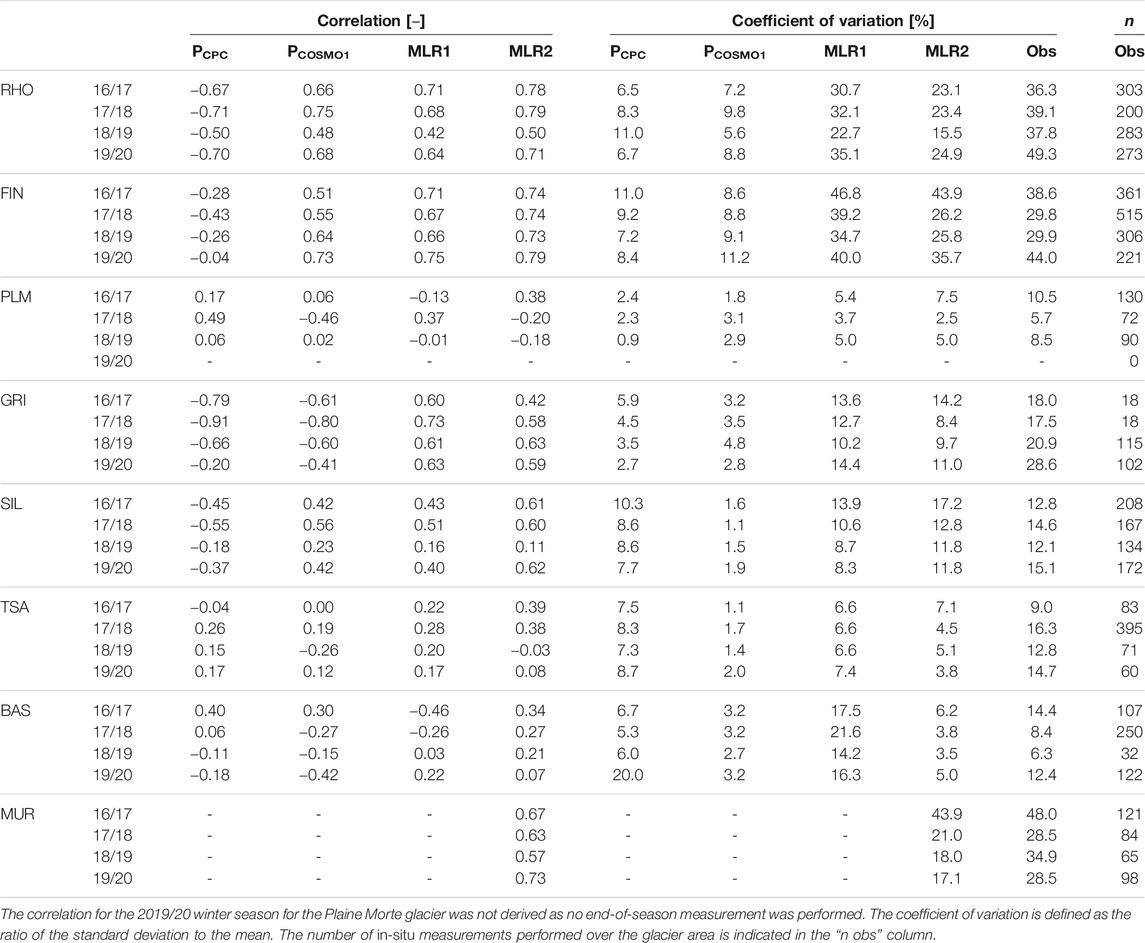
TABLE 4. CombiPrecip, COSMO-1 precipitation, Step-1 model (MLR1) and Step-2 model (MLR2) correlations with respect to end-of-season in-situ measurements, for all the glaciers and all the winter seasons.

In addition, the small surface extent of the Basòdino and Silvretta glaciers, that is, of 1.8 and 2.6 km², respectively, also influences the results, as these glaciers are only covered by a few original CombiPrecip or COSMO-1 data grid cells. Furthermore, no correlation was computed for Murtèl, because the glacier is only represented by one single grid cell (i.e., there is no spatial variability). Figure 7 further highlights the great underestimation of the precipitation products, where, in addition to the radar visibility, other effects also need to be considered.

5.2 The Importance of and Dependency on the CRS Data

Step-1 MLR was trained using Plaine Morte CRS data and cannot therefore be considered independent of direct field measurements. On the other hand, Step-2 MLR was built completely according to a “leave-one-glacier-out” cross-validation process. The Step-1 MLR estimates that were re-adjusted in Step-2 MLR thus only consider measurements from the other seven glaciers and the relative local topography. The final results of Step-2 MLR are therefore independent of any direct in-situ measurements. As shown in Figure 9, the resulting SWE estimates from Step-2 MLR agree well with the CRS observations and field measurements of Plaine Morte and Findel (Findel is a completely independent test site for Step-1 MLR too) for most of the winter seasons. This implies that our model is suitable for applications at smaller timescales than seasonal, without any evident loss in performance.

5.3 Wind and Radiation Components

Glaciers only form where snow can survive for several summer seasons, together with an above-average precipitation catch, due to topographic-meteorologic interactions and/or additional snow accumulation resulting from the re-distribution of snow by avalanches or wind (e.g., Kuhn, 1995; Trujillo et al., 2007; Lehning et al., 2008; Mott et al., 2019). These processes cannot be represented by simply accumulating the observed precipitations over the glacier area. Given the multiple issues involved in determining precipitation amounts at these high altitudes, our approach is not able to link advection distances with wind speed. Nevertheless, including the wind speed variable in Step-1 MLR allowed the correlation with ground measurements to be greatly improved for most glaciers (cf. Table 4 positive correlation was estimated over the Gries glacier for all the winter seasons, when the spatial distribution of both cumulative COSMO-1 and CombiPrecip was negatively correlated with the in-situ SWE measurements. Our result confirms that high horizontal wind speeds at mountain crests play a key role in the final distribution of snowfall and snow deposition. In fact, such winds influence the advection of falling snow particles downstream (e.g., Colle, 2004; Zängl, 2008; Mott et al., 2014). Dadic et al. (2010) found that downward winds cause an increased deposition in the lee of mountain ridges, where winds are usually stronger than over the flatter areas of a glacier. This could further explain our results, which indicate a positive correlation between wind speed and SWE. Snow melt and sublimation are other processes that modify a snowpack, and higher temperatures in early spring further reduce the SWE measured at the end of the season (e.g., Pohl et al., 2006; Mott et al., 2011; DeBeer and Pomeroy, 2017) and thus could partially explain the increase in the ratios between the cumulative estimates of all the considered precipitation products and the ground measurements from 2017/2018 to 2019/2020 (cf. Figure 7). Moreover, the ratio that is constantly around 1 in the same figure confirms the general validity of Step-1 MLR given by Eq. 1 for all eight glaciers considered in this study, although based only on CRS observations from the Plaine Morte glacier. Step-2 MLR shows very similar ratios.

5.4 Influence of the Local Topography on the SWE Distribution

Previous studies have demonstrated that high-resolution topographical parameters are necessary to represent the small-scale snow distribution. In fact, Molotch and Bales (2005) analyzed the spatial distribution of SWE within grid elements of various resolutions (16, 4, and 1 km²) surrounding some snow telemetry (SNOTEL) sites in the Rio Grande headwaters in the United States. In some cases, SNOTEL SWE values were 200% greater than the mean SWE grid value. To analyze the relationships between topographical parameters and snow accumulation on specific sites, several studies used statistical models such as regression trees and MLR (e.g., Elder et al., 1998; Balk and Elder, 2000; Erxleben et al., 2002; Winstral et al., 2002; Anderton et al., 2004; Jost et al., 2007; Litaor et al., 2008; Grünewald et al., 2013).

In our study, we compare the variability of point-scale in-situ SWE measurements with the variability of the gridded precipitation products CombiPrecip and COSMO-1, and with the variability of the two-step MLR model, which only uses topographical parameters in order to increase its applicability to independent sites. The boxplots shown in Figures 8A,D,G indicate that CombiPrecip and COSMO-1 precipitation estimates do not represent the larger spatial variability of the in-situ SWE measurements over the glacier area of Findel glacier. The coefficients of variation reported in Table 4 indicate that the reduced spatial variability of the cumulative precipitation of CombiPrecip and COSMO-1, compared with the variability of the in-situ SWE measurements, is also observed for other glaciers. The variability of the in-situ SWE measurements at a higher spatial resolution than 1 × 1 km² can partially be explained by Step-2 MLR, as a result of including the topographical parameters. In fact, the correlation scores in Table 4 and Figure 8 indicate that Step-2 MLR results in higher spatial correlations with in-situ SWE measurements. Our results are in line with observed snow accumulation processes in mountain topography, where precipitation patterns at the mountain-ridge scale are mainly dominated by terrain and wind-driven processes acting at a small scale (Gerber et al., 2018; Mott et al., 2018). Scipión et al. (2013) compared the variability of continuous small-scale precipitation observations of a polarimetric X-band radar with local measurements of snow accumulation, collected by means of airborne laser-scanning. They also concluded that the variability of snow accumulation, at smaller scales than a few kilometers, is affected by snow redistribution processes, and that topographically induced wind patterns have a great influence on snow accumulation. The importance of the inclusion of the topographical parameters in Step-2 MLR is further highlighted in Figure 5, which shows that when such parameters are not involved (Step-1 MLR), the model underestimates the ground measurements for negative TPI₂₂₅ values (concave areas). This is a result of increased snow accumulating in concave areas, which has been shown in previous studies (e.g., Revuelto et al., 2014; Schöber et al., 2014). Our Step-2 MLR uses TPI parameters that are also representative of larger spatial scales (derived from square moving windows of 525 × 525, 1,025 × 1,025, and 2,025 × 2,025 m sizes). However, their inclusion in Step-2 MLR may also be due to the relationship between TPI and COSMO-1 wind field errors. In fact, in this regard, Winstral et al. (2017) found that COSMO-2 and COSMO-7 (2 and 7 km of horizontal resolution) overestimated the measured wind speed in valleys and overestimated it over upper slopes and ridges.

5.5 Non-glacierized Areas

Our Step-2 model has been shown to provide reliable temporal and spatial SWE estimates over Swiss glaciers, and it is thus supposed it will provide comparable performance for regions with similar topographical characteristics. However, the application of Step-2 MLR to lower elevations and non-glacierized mountain areas, remains a challenging task. The morphology of the terrain around the non-glacierized sites is in general more complex (e.g., narrow valleys, close to ridges) than at the glacier sites (training data), which in turn leads to extrapolation problems of linear regressions. The majority of the non-glacierized sites in our study are also located at lower elevation than the average altitude of the eight glaciers, which leads to an earlier onset of snow melt and/or midwinter ablation events due to higher air temperatures. Moreover, the observed positive correlation between wind and snow amounts over glaciers is not transferable to each and every location in the Swiss Alps, because some more exposed areas may lose snow as a result of wind drift processes. Furthermore, precipitation-only products perform better in non-glacierized areas than in the glacier areas analyzed in this study. The overall higher values of COSMO-1 and CombiPrecip than of the field measurements (cf. Figure 10 and Figure 11) may suggest that our MLR models generally lead to too high values, since the precipitation estimates are scaled (and increased) by the coefficients of the MLRs. The reduced ratio between ground observations and precipitation may be explained by the SWE decrease caused by sublimation, melt and sometimes rain events, which increase the cumulative precipitation, but not the SWE. This is probably also the case for low elevated sites (e.g., Supplementary Figure S8A (17/18), Supplementary Figures S9B,S9D (19/20) and Supplementary Figure S12C). However, rain or meltwater would refreeze in a sufficiently deep snowpack, without any additional runoff, thus increasing the SWE. The high values observed for Weissfluhjoch (Figure 11E) may be caused by the fact that this station is located within a distance of less than 1 km from the major ridge, where the COSMO-1 wind is strong and the model therefore produces too much snow.

A great advantage of Step-2 MLR, compared to precipitation-only products, is thus its ability to model negative variations given by the negative correlation with certain topographical parameters and the negative constant included in Step-1 MLR. However, the negative constant, combined with weak winds at low stations, can also lead to frequent underestimations, as can clearly be seen for the Step-1 estimates in Figures 11A,D. In fact, Eq. 1 implies that if no precipitation occurs and the hourly wind speed is lower than 4.17 ms, Step-1 MLR would predict a loss of SWE. Discrepancies between Step-1 and Step-2MLRs are related to the influence of the local topography, but also to the greater weight of the COSMO-1 estimates in Step-2 MLR (cf. Eq. 9) and to the consequent lower weight given to the wind speed.

In general, we to conclude that even though the majority of non-glacierized sites are located at lower elevations, Step-2 MLR still produces good estimates with a performance that is comparable with that of COSMO-1 and CombiPrecip. However, the MLR models are not able to predict marked SWE losses, because they are calibrated with snow measurements over glaciers, where the snow melt is weaker than on low elevated sites.

5.6 Overall Analyses of the Model Approach

5.6.1 Step-1 Model

The choice of using Plaine Morte instead of Findel as the reference glacier and thus as the model training site was based on the longer CRS time series, the very good radar visibility due to a weather radar being located directly on the Pointe de la Plaine Morte (Gugerli et al., 2020) and the topographic characteristic of the glacier, with nearly no elevation gradients (2,470 m.a.s.l. to 2,828 m.a.s.l.). Thus, we assumed that the amount of SWE is mostly due to direct snowfall and only marginally influenced by other snow accumulation processes, such as snow drift or avalanches. More complex model setups were tested for Step-1 MLR. For instance, we considered COSMO-1 temperatures (2 and 10 m from the ground), but their inclusion in the statistical model led to large errors when the model was applied to the test site (Findel). Our resulting Step-1 MLR model (cf. Eq. 1) indicates that COSMO-1 and CombiPrecip estimates are combined, with more weight being assigned to COSMO-1 precipitation estimates. The fact that the standard error and the confidence interval in Table 2 are quite large for both COSMO-1 precipitation and CombiPrecip indicates that the model is challenged to find an optimal balance between these two precipitation estimates, as they are closely correlated with each other. However, including both variables in the MLR led to better results. The positive coefficient of the wind speed component suggests that stronger winds over the Plaine Morte glacier result in higher precipitation on the glacier being transferred from the surrounding area and/or snow being moved to the CRS location by snow drift processes. In addition, the model involves a negative constant term, which regroups all the processes that cannot be modeled with our explaining variables (such as SWE losses, but also the average noise within the CRS observations (cf. Gugerli et al., 2019)), thereby resulting in an average negative variation of SWE.

5.6.2 Step-2 Model

Problems of extrapolating Step-2 MLR to regions characterized by a topography that is very different from the topography of the glaciers, such as the non-glacierized sites considered in this study, may arise. In particular, because of the overall limited heterogeneity of topography of glaciers, only a few measurements are available for glacier areas with a lower TPI₂₂₅ than −15 and higher than 15 m (seeFigure 5), consequently, the extrapolation of the observed linear relation to larger absolute TPI₂₂₅ values could lead to large errors. In order to partially solve such extrapolation issues, it would be possible to flatten the regression from defined thresholds, depending on the training data. Moreover, the exposition of terrain to the Sun allows the precipitation estimates to be corrected as snow melt processes can be taken into consideration. However, snow melt processes are probably more important at the lower elevated non-glacierized sites (test data) than at the glacier sites (training and validation data). Furthermore, our model cannot account for strong snow melt processes occurring during rain-on-snow events, caused by the effects of turbulent heat fluxes (e.g., Schlögl et al., 2018). Other studies have included such indicators as elevation or wind-sheltering parameters in their statistical models (Winstral et al., 2002; Molotch and Bales, 2005; Grünewald et al., 2013). In our case, we could not use such parameters because they would have negatively affected the possibility of generalizing the MLR model.

It would of course be possible to build more complex and specific models, adapted to each different glacier, similarly to what Grünewald et al. (2013) did. However, our goal was to extrapolate the new SWE estimates to regions with no ground observations, and we therefore built a single model with good generalization scores.

5.6.3 Limits of the Overall Approach

More advanced machine learning models that allow modeling non-linear relationships, could lead to an even better performance of the model. We made a tentative experiment to create a more accurate universal model by building a model tree, which combined decision trees with MLRs. Such a model tree minimizes the mean squared error with respect to the measurements, and thus builds a tree composed of a different MLR at the end of each branch.

In our case, only topographical parameters were considered as decision variables, while dynamical variables such as precipitation, wind and temperature, were combined with different MLRs. Such advanced models can also be trained and applied at different timescales, with the advantage of being able to model non-linear relationships by dividing the data according to their characteristics (topographical), and to create a different MLR for each data subset. However, we were not able to build a universal model that provided very good performance on both glaciers and lower elevated non-glacierized sites. The main reason for this is related to the different topographies and altitudes of the two datasets: on the one hand, glaciers are located at higher altitudes and the model tree was not able to create an MLR that could be adapted to lower altitudes and to the more complex topography of the non-glacierized sites, and on the other hand, the absence of several stations at very high altitudes with similar topographical characteristics to glaciers, did not allow us to create a model tree based on the twice-monthly manual measurements, and then apply it over glacier areas with satisfactory results. This was further complicated by the different temporal scales between the measurements performed at the glacierized sites (seasonal) and non-glacierized sites (twice a month). In order to create a universal model, a more topographically diversified dataset with proportionate measurements, would thus be needed.

6 Conclusion

Our statistically based model, built with multiple data sources, has allowed spatial and temporal highly resolved SWE estimates to be estimated in remote high-mountain regions, with a good agreement with manual in-situ measurements. The use of such statistical models as MLRs has proven to be particularly appropriate to combine different types of data from distinct sources and with various spatio-temporal resolutions. However, end-of-season scattered SWE measurements, used to model the overall processes, and the availability of evenly distributed measurements, carried out at shorter time distances, would make it possible to conduct more detailed analyses. In fact, the use of cumulative values for each variable does not allow complex processes (e.g., wind driven), acting at small spatial and temporal scales, as described by Mott et al. (2018), to be clearly identified and modeled.

This study confirms the importance of high-resolution topographical information to explain preferential deposition processes at small spatial scales. In our approach, the use of high-resolution topography was necessary to relate the precipitation over a squared km with the point SWE measurements on the ground. Moreover, TPI was an important parameter to overcome the differences between precipitation estimates and ground SWE measurements over glaciers, and larger accumulations were identified in concavities compared to terrain convexities. Furthermore, our solar radiation parameter allowed us to take into account that a snowpack is affected less by melting and sublimation processes in more shaded areas. Finally, larger precipitation amounts on the glacier surface appear to be related to stronger winds. This could be due to downward winds, which cause an increased deposition in the lee of mountain ridges, where winds are usually stronger than at lower elevations of glaciers. However, this relationship was not always confirmed for non-glacierized sites located in areas characterized by a different terrain morphology (e.g., Comola et al., 2019).

The good performance of the model shown in this study, and its proven application to glaciers without any input data and even for non-glacierized sites, makes our approach a promising tool for advances in glaciology, hydrology, and generally in the evaluation of precipitation products. The continuous, highly resolved evolution of snow accumulation over glaciers is currently rarely studied, as observations are usually only available at a seasonal resolution (e.g., Dadic et al., 2010; Helfricht et al., 2014; Gugerli et al., 2019). Our approach enables the understanding of the temporal evolution of snow accumulation and its impacts on glacier dynamics to be improved.

Currently, the model can be applied to the entire Swiss Alps with a spatial resolution of 25 × 25 m² and improved estimates on glacier areas. However, its application to lower elevated non-glacierized sites remains limited by the more complex topography and by strong melt events reducing the SWE during the winter season. In order to extend it to regions outside the Swiss boundaries, high-resolution topography and spatio-temporally resolved precipitation and wind speed estimates are needed from any target regions.

In general, our approach can be further developed and could be integrated with other precipitation products. For instance, the adjustment of global precipitation data could be used to improve high-altitude precipitation estimates over regions with very scarce data availability, like Central Asia and the Himalayas. Results generated by our model could also directly be used as a reference for the post-processing of global circulation models, thus allowing future scenarios to be re-evaluated and consistently improving our knowledge about precipitations and their evolution at very high altitudes.

Data Availability Statement

Publicly available datasets were analyzed in this study. The analyzed CombiPrecip and COSMO-1 data are available from MeteoSwiss, while the CRS observations will soon be available in a repository. The glaciological end-of-season surveys of GLAMOS are freely available at https://www.glamos.ch/en/. The twice-monthly SWE measurements of 11 SLF stations (non-glacierized sites) can be downloaded free of charge at https://www.envidat.ch/dataset/gcos-swe-data.

Author Contributions

MGu wrote the article, conducted the data analysis and modeling and defined the details of the concept of the study; RG and NS established the first guidelines of the study and helped with continuous discussions concerning the results; MGa contributed to the analysis of radar-composite estimates; CM prepared the non-glacierized sites data and contributed to the evaluation of the related results; all the authors contributed to improving the article.

Funding

The study is part of the High-SPA 200021_178963 project, which is funded by the Swiss National Science Foundation (SNSF).

Conflict of Interest

The authors declare that the research was conducted in the absence of any commercial or financial relationships that could be construed as a potential conflict of interest.

Acknowledgments

Special thanks are due to MeteoSwiss, GLAMOS and SLF for providing their data, in particular to Daniel Wolfensberger (MeteoSwiss) for supporting in preparing the CombiPrecip data, Daniel Leuenberger (MeteoSwiss) for supporting in preparing the COSMO-1 data and Matthias Huss (GLAMOS) for providing the end-of-season in-situ measurements data of the eight glaciers considered in this study.

Supplementary Material

The Supplementary Material for this article can be found online at: https://www.frontiersin.org/articles/10.3389/feart.2021.664648/full#supplementary-material

References

Anderton, S. P., White, S. M., and Alvera, B. (2004). Evaluation of Spatial Variability in Snow Water Equivalent for a High Mountain Catchment. Hydrological Process. 18, 435–453. doi:10.1002/hyp.1319
Balk, B., and Elder, K. (2000). Combining Binary Decision Tree and Geostatistical Methods to Estimate Snow Distribution in a Mountain Watershed. Water Resour. Res. 36, 13–26. doi:10.1002/hyp.1319
Bernhardt, M., and Schulz, K. (2010). SnowSlide: A Simple Routine for Calculating Gravitational Snow Transport. Geophys. Res. Lett. 37, L11502. doi:10.1029/2010GL043086
Cline, D., Elder, K., and Bales, R. (1998). Scale Effects in a Distributed Snow Water Equivalence and Snowmelt Model for Mountain Basins. Hydrological Process. 12, 1527–1536. doi:10.1002/(SICI)1099-1085(199808/09)12:10/11<1527::AID-HYP678>3.0.CO;2-E
Colle, B. A. (2004). Sensitivity of Orographic Precipitation to Changing Ambient Conditions and Terrain Geometries: An Idealized Modeling Perspective. J. Atmos. Sci. 61, 588–606. doi:10.1175/1520-0469(2004)061<0588:SOOPTC>2.0.CO;2
Comola, F., Giometto, M. G., Salesky, S. T., Parlange, M. B., and Lehning, M. (2019). Preferential Deposition of Snow and Dust Over Hills: Governing Processes and Relevant Scales. J. Geophys. Res. Atmospheres 124, 7951–7974. doi:10.1029/2018JD029614
Dadic, R., Mott, R., Lehning, M., and Burlando, P. (2010). Wind Influence on Snow Depth Distribution and Accumulation over Glaciers. J. Geophys. Res. Earth Surf. 115, 587–601. doi:10.1029/2009JF001261
DeBeer, C. M., and Pomeroy, J. W. (2017). Influence of Snowpack and Melt Energy Heterogeneity on Snow Cover Depletion and Snowmelt Runoff Simulation in a Cold Mountain Environment. J. Hydrol. 553, 199–213. doi:10.1016/j.jhydrol.2017.07.051
Egli, L., Jonas, T., and Meister, R. (2009). Comparison of Different Automatic Methods for Estimating Snow Water Equivalent. Cold Regions Sci. Tech. 57, 107–115. doi:10.1016/j.coldregions.2009.02.008
Elder, K., Rosenthal, W., and Davis, R. E. (1998). Estimating the Spatial Distribution of Snow Water Equivalence in a Montane Watershed. Hydrological Process. 12, 1793–1808. doi:10.1002/(SICI)1099-1085(199808/09)12:10/11<1793::AID-HYP695>3.0.CO;2-K
Erxleben, J., Elder, K., and Davis, R. (2002). Comparison of Spatial Interpolation Methods for Estimating Snow Distribution in the Colorado Rocky Mountains. Hydrological Process. 16, 3627–3649. doi:10.1002/hyp.1239
Fortin, V., Therrien, C., and Anctil, F. (2008). Correcting Wind–Induced Bias in Solid Precipitation Measurements in Case of Limited and Uncertain Data. Hydrological Process. 22, 3393–3402. doi:10.1002/hyp.6959
Fujita, K. (2008). Effect of Precipitation Seasonality on Climatic Sensitivity of Glacier Mass Balance. Earth Planet. Sci. Lett. 276, 14–19. doi:10.1016/j.epsl.2008.08.028
Gabella, M. (2004). Improving Operational Measurement of Precipitation Using Radar in Mountainous Terrain-Part II: Verification and Applications. IEEE Geosci. Remote Sensing Lett. 1, 84–89. doi:10.1109/LGRS.2003.823294
Gabella, M., Joss, J., and Perona, G. (2000). Optimizing Quantitative Precipitation Estimates Using a Noncoherent and a Coherent Radar Operating on the Same Area. J. Geophys. Res. Atmospheres 105, 2237–2245. doi:10.1029/1999JD900420
Gabella, M., Speirs, P., Hamann, U., Germann, U., and Berne, A. (2017). Measurement of Precipitation in the Alps Using Dual-Polarization C-Band Ground-Based Radars, the GPM Spaceborne Ku-Band Radar, and Rain Gauges. Remote Sensing 9, 1147. doi:10.3390/rs9111147
Gauer, P. (2001). Numerical Modeling of Blowing and Drifting Snow in Alpine Terrain. J. Glaciology 47, 97–100. doi:10.3189/172756501781832476
Gerber, F., Besic, N., Sharma, V., Mott, R., Daniels, M., Gabella, M., et al. (2018). Spatial Variability in Snow Precipitation and Accumulation in COSMO–WRF Simulations and Radar Estimations over Complex Terrain. Cryosphere 12, 3137–3160. doi:10.5194/tc-12-3137-2018
Gerber, F., Mott, R., and Lehning, M. (2019). The Importance of Near-Surface Winter Precipitation Processes in Complex Alpine Terrain. J. Hydrometeorology 20, 77–96. doi:10.1175/JHM-D-18-0055.1
Germann, U., Galli, G., Boscacci, M., and Bolliger, M. (2006). Radar Precipitation Measurement in a Mountainous Region. Q. J. od R. Meteorol. Soc. 132, 1669–1692. doi:10.1256/qj.05.190
Germann, U., and Joss, J. (2004). “Operational Measurement of Precipitation in Mountainous Terrain,” in Weather Radar. Physics of Earth and Space Environments. Editor P. Meischner (Berlin: Springer), 52–77. doi:10.1007/978-3-662-05202-0_2
GLAMOS (2018). The Swiss Glaciers 2015/16 and 2016/17: Glaciological Report No. 137/138. “Yearbooks Of the Cryospheric Commission Of the Swiss Academy Of Sciences (SCNAT),” published since 1964 by VAW/ETH Zurich. doi:10.18752/glrep_137-13
Goodison, B. E., Louie, P. Y. T., and Yang, D. (1998). WMO Solid Precipitation Measurement Intercomparison Final Report. World Meteorol. Organ. WMO/Tech. 872, 212, Available at: https://www.wmo.int/pages/prog/www/IMOP/publications/IOM-67-solid-precip/WMOtd872.pdfr
Gruber, S. (2007). A Mass–Conserving Fast Algorithm to Parameterize Gravitational Transport and Deposition Using Digital Elevation Models. Water Resour. Res. 43, W06412. doi:10.1029/2006wr004868
Grünewald, T., Bühler, Y., and Lehning, M. (2014). Elevation Dependency of Mountain Snow Depth. The Cryosphere 8, 2381–2394. doi:10.5194/tc-8-2381-2014
Grünewald, T., Stötter, J., Pomeroy, J. W., Dadic, R., Baños, I. M., Marturià, J., et al. (2013). Statistical Modelling of the Snow Depth Distribution in Open Alpine Terrain. Hydrol. Earth Syst. Sci. 17, 3005–3021. doi:10.5194/hess-17-3005-2013
Grüter, E., Abbt, M., Häberli, C., Häller, E., Küng, U., Musa, M., et al. (2003). Quality Control Tools for Meteorological Data in the MeteoSwiss Data Warehouse System. Internal Report. MeteoSwiss.
Gugerli, R., Gabella, M., Huss, M., and Salzmann, N. (2020). Can Weather Radars Be Used to Estimate Snow Accumulation on Alpine Glaciers? - an Evaluation Based on Glaciological Surveys. J. Hydrometeorology 21, 2943–2962. doi:10.1175/JHM-D-20-0112.1
Gugerli, R., Guidicelli, M., Gabella, M., Huss, M., and Salzmann, N. (2021). Multi-sensor Analysis of Monthly Gridded Snow Precipitation on Alpine Glaciers. Adv. Sci. Res. 18, 7–20. doi:10.5194/asr-18-7-2021
Gugerli, R., Salzmann, N., Huss, M., and Desilets, D. (2019). Continuous and Autonomous Snow Water Equivalent Measurements by a Cosmic Ray Sensor on an Alpine Glacier. The Cryosphere 13, 3413–3434. doi:10.5194/tc-13-3413-2019
Helfricht, K., Kuhn, M., Keuschnig, M., and Heilig, A. (2014). Lidar Snow Cover Studies on Glaciers in the Ötztal Alps (Austria): Comparison with Snow Depths Calculated from GPR Measurements. The Cryosphere 8, 41–57. doi:10.5194/tc-8-41-2014
Hock, R., Hutchings, J. K., and Lehning, M. (2017). Grand Challenges in Cryospheric Sciences: Toward Better Predictability of Glaciers, Snow and Sea Ice. Front. Earth Sci. 5, 64. doi:10.3389/feart.2017.00064
Howat, I. M., de la Peña, S., Desilets, D., and Womack, G. (2018). Autonomous Ice Sheet Surface Mass Balance Measurements from Cosmic Rays. The Cryosphere 12, 2099–2108. doi:10.5194/tc-12-2099-2018
Huss, M., Dhulst, L., and Bauder, A. (2015). New Long-Term Mass-Balance Series for the Swiss Alps. J. Glaciology 61, 551–562. doi:10.3189/2015JoG15J015
Ikeda, K., Rasmussena, R., Liu, C., Gochis, D., Yates, D., Chen, F., et al. (2010). Simulation of Seasonal Snowfall over Colorado. Atmos. Res. 97, 462–477. doi:10.1016/j.atmosres.2010.04.010
Jonas, T., Marty, C., and Magnusson, J. (2009). Estimating the Snow Water Equivalent from Snow Depth Measurements in the Swiss Alps. J. Hydrol. 378, 161–167. doi:10.1016/j.jhydrol.2009.09.021
Joss, J., and Waldvogel, A. (1990). in “Precipitation Measurements and Hydrology,” in Radar in Meteorology. Editor D. Atlas (Boston, MA: American Meteorological Society), 577–606. doi:10.1007/978-1-935704-15-7–39
Jost, G., Weiler, M., Gluns, D. R., and Alila, Y. (2007). The Influence of Forest and Topography on Snow Accumulation and Melt at the Watershed-Scale. J. Hydrol. 347, 101–115. doi:10.1016/j.jhydrol.2007.09.006
Kerr, T., Clark, M., Hendrikx, J., and Anderson, B. (2013). Snow Distribution in a Steep Mid-latitude Alpine Catchment. Adv. Water Resour. 55, 17–24. doi:10.1016/j.advwatres.2012.12.010
Kobold, M., and Sušelj, K. (2005). Precipitation Forecasts and Their Uncertainty as Input into Hydrological Models. Hydrol. Earth Syst. Sci. 9, 322–332. doi:10.5194/hess-9-322-2005
Kochendorfer, J., Rasmussen, R., Wolff, M., Baker, B., Hall, M. E., Meyers, T., et al. (2017). The Quantification and Correction of Wind-Induced Precipitation Measurement Errors. Hydrol. Earth Syst. Sci. 21, 1973–1989. doi:10.5194/hess-21-1973-2017
Kodama, M. (1980). Continuous Monitoring of Snow Water Equivalent Using Cosmic-Ray Neutrons. Cold Regions Sci. Tech. 3, 295–303. doi:10.1016/0165-232X(80)90036-1
Kopp, G., and Lean, J. L. (2011). A New, Lower Value of Total Solar Irradiance: Evidence and Climate Significance. Geophys. Res. Lett. 38, L01706. doi:10.1029/2010GL045777
Lehning, M., Bartelt, P., Brown, B., Russi, T., Stöckli, U., and Zimmerli, M. (1999). SNOWPACK Model Calculations for Avalanche Warning Based upon a Network of Weather and Snow Stations. Cold Regions Sci. Tech. 30, 145–157. doi:10.1016/S0165-232X(99)00022-1
Lehning, M., Löwe, H., Ryser, M., and Raderschall, N. (2008). Inhomogeneous Precipitation Distribution and Snow Transport in Steep Terrain. Water Resour. Res. 44, W07404. doi:10.1029/2007WR006544
Litaor, M. I., Williams, M., and Seastedt, T. R. (2008). Topographic Controls on Snow Distribution, Soil Moisture, and Species Diversity of Herbaceous Alpine Vegetation, Niwot Ridge, Colorado. J. Geophys. Res. Biogeosciences 113, G02008. doi:10.1029/2007jg000419
López–Moreno, J. I., Leppänen, L., Luks, B., Holko, L., Picard, G., Sanmiguel–Vallelado, A., et al. (2020). Intercomparison of Measurements of Bulk Snow Density and Water Equivalent of Snow Cover with Snow Core Samplers: Instrumental Bias and Variability Induced by Observers. Hydrological Process. 34, 3120–3133. doi:10.1002/hyp.13785
López–Moreno, J. I., and Nogués–Bravo, D. (2006). Interpolating Local Snow Depth Data: An Evaluation of Methods. Hydrological Process. 20, 2217–2232. doi:10.1002/Hyp.6199
Marty, C. (2017). GCOS SWE Data from 11 Stations in Switzerland. Davos, Switzerland: WSL Institute for Snow and Avalanche Research SLF. doi:10.16904/15
MeteoSwiss (2018). Documentation of MeteoSwiss Grid-Data Products. Hourly Precipitation Estimation through Rain-Gauge and Radar: CombiPrecip. Available at: https://www.meteoschweiz.admin.ch/content/dam/meteoswiss/en/climate/swiss-climate-in-detail/doc/ProdDoc_CPC.pdf (Accessed December 12, 2020).
MeteoSwiss (2016). The New Weather Forecasting Model for the Alpine Region. Available at: https://www.meteoswiss.admin.ch/home/latest-news/news.subpage.html/en/data/news/2016/3/the-new-weather-forecasting-model-for-the-alpine-region.html (Accessed December 12, 2020).
Molotch, M. P., and Bales, R. C. (2005). Scaling Snow Observations from the Point to the Grid Element: Implications for Observation Network Design. Water Resour. Res. 41, W11421. doi:10.1029/2005WR004229
Mott, R., Egli, L., Grünewald, T., Dawes, N., Manes, C., Bavay, M., et al. (2011). Micrometeorological Processes Driving Snow Ablation in an Alpine Catchment. The Cryosphere 5, 1083–1098. doi:10.5194/tc-5-1083-2011
Mott, R., Schirmer, M., Bavay, M., Grünewald, T., and Lehning, M. (2010). Understanding Snow-Transport Processes Shaping the Mountain Snow-Cover. The Cryosphere 4, 545–559. doi:10.5194/tc-4-545-2010
Mott, R., Scipión, D., Schneebeli, M., Dawes, N., Berne, A., and Lehning, M. (2014). Orographic Effects on Snow Deposition Patterns in Mountainous Terrain. J. Geophys. Res. Atmospheres 119, 1419–1439. doi:10.1002/2013JD019880
Mott, R., Vionnet, V., and Grünewald, T. (2018). The Seasonal Snow Cover Dynamics: Review on Wind-Driven Coupling Processes. Front. Earth Sci. 6, 197. doi:10.3389/feart.2018.00197
Mott, R., Wolf, A., Kehl, M., Kunstmann, H., Warscher, M., and Grünewald, T. (2019). Avalanches and Micrometeorology Driving Mass and Energy Balance of the Lowest Perennial Ice Field of the Alps: a Case Study. The Cryosphere 13, 1247–1265. doi:10.5194/tc-13-1247-2019
Pohl, S., Marsh, P., and Liston, G. E. (2006). Spatial-Temporal Variability in Turbulent Fluxes during Spring Snowmelt. Arctic, Antarctic, Alpine Res. 38, 136–146. doi:10.1657/1523-0430(2006)038[0136:SVITFD]2.0.CO;2
Pollock, M. D., O’Donnell, G., Quinn, P., Dutton, M., Black, A., Wilkinson, M. E., et al. (2013). Quantifying and Mitigating Wind–Induced Undercatch in Rainfall Measurements. Water Resour. Res. 54, 3863–3875. doi:10.1029/2017WR022421
Pomeroy, J. W., and Gray, D. M. (1995). Snowcover Accumulation, Relocation and Management. Saskatoon, Canada: National Hydrology Research Institute Science Report.
Rasmussen, R., Baker, B., Kochendorfer, J., Meyers, T., Landolt, S., Fischer, A. P., et al. (2012). How Well Are We Measuring Snow? the NOAA/FAA/NCAR Winter Precipitation Test Bed. Bull. Amer. Meteorol. Soc. 93, 811–829. doi:10.1175/BAMS-D-11-00052.1
Revuelto, J., López-Moreno, J. I., Azorin-Molina, C., and Vicente-Serrano, S. M. (2014). Topographic Control of Snowpack Distribution in a Small Catchment in the Central Spanish Pyrenees: Intra- and Inter-annual Persistence. The Cryosphere 8, 1989–2006. doi:10.5194/tc-8-1989-2014
Rohrer, M. B., Braun, L. N., and Lang, H. (1994). Long-Term Records of Snow Cover Water Equivalent in the Swiss Alps 1. Analysis. Nordic Hydrol. 25, 53–64. doi:10.2166/nh.1994.0019
Saltikoff, E., Lopez, P., Taskinen, A., and Pulkkinen, S. (2015). Comparison of Quantitative Snowfall Estimates from Weather Radar, Rain Gauges and a Numerical Weather Prediction Model. Boreal Environ. Res. 20, 667–678.
Salzmann, N., Huggel, C., Rohrer, M., and Stoffel, M. (2014). Data and Knowledge Gaps in Glacier, Snow and Related Runoff Research – A Climate Change Adaptation Perspective. J. Hydrol. 518, 225–234. doi:10.1016/j.jhydrol.2014.05.058
Schirmer, M., and Jamieson, B. (2015). Verification of Analysed and Forecasted Winter Precipitation in Complex Terrain. The Cryosphere 9, 587–601. doi:10.5194/tc-9-587-2015
Schlögl, S., Lehning, M., and Mott, R. (2018). How Are Turbulent Sensible Heat Fluxes and Snow Melt Rates Affected by a Changing Snow Cover Fraction?. Front. Earth Sci. 6, 154. doi:10.3389/feart.2018.00154
Schöber, J., Schneider, K., Helfricht, K., Schattan, P., Achleitner, S., Schöberl, F., et al. (2014). Snow Cover Characteristics in a Glacierized Catchment in the Tyrolean Alps - Improved Spatially Distributed Modelling by Usage of Lidar Data. J. Hydrol. 519, 3492–3510. doi:10.1016/j.jhydrol.2013.12.054
Scipión, D. E., Mott, R., Lehning, M., Schneebeli, M., and Berne, A. (2013). Seasonal Small-Scale Spatial Variability in Alpine Snowfall and Snow Accumulation. Water Resour. Res. 49, 1446–1457. doi:10.1002/wrcr.20135
Seiz, G., Foppa, N., Meier, M., and Meister, O. (2010). National Climate Observing System (GCOS Switzerland). Adv. Sci. Res. 6. doi:10.5194/asr-6-95-2011
Sideris, I. V., Gabella, M., Erdin, R., and Germann, U. (2014). Real–time Radar–Rain–Gauge Merging Using Spatio–Temporal Co–kriging with External Drift in the Alpine Terrain of Switzerland. Q. J. R. Meteorol. Soc. 140, 1097–1111. doi:10.1002/qj.2188
Sigouin, M. J. P., and Si, B. C. (2016). Calibration of a Non-invasive Cosmic-Ray Probe for Wide Area Snow Water Equivalent Measurement. The Cryosphere 10, 1181–1190. doi:10.5194/tc-10-1181-2016
Sugiura, K., Yang, D., and Ohata, T. (2003). Systematic Error Aspects of Gauge-Measured Solid Precipitation in the Arctic, Barrow, Alaska. Geophys. Res. Lett. 30, 1192. doi:10.1029/2002GL015547
Tapiador, F. J., Turk, F. J., Petersen, W., Hou, A. Y., García-Ortega, E., Machado, L. A. T., et al. (2012). Global Precipitation Measurement: Methods, Datasets and Applications. Atmos. Res. 104-105, 70–97. doi:10.1016/j.atmosres.2011.10.021
Trujillo, E., Ramírez, J. A., and Elder, K. J. (2007). Topographic, Meteorologic, and Canopy Controls on the Scaling Characteristics of the Spatial Distribution of Snow Depth Fields. Water Resour. Res. 43, W07409. doi:10.1029/2006WR005317
Wastl, C., and Zängl, G. (2008). Analysis of Mountain-Valley Precipitation Differences in the Alps. Meteorologische Z. 17, 311–321. doi:10.1127/0941-2948/2008/0291
Weusthoff, T., Ament, F., Arpagaus, M., and Rotach, M. W. (2010). Assessing the Benefits of Convection-Permitting Models by Neighborhood Verification: Examples from MAP D-PHASE. Monthly Weather Rev. 138, 3418–3433. doi:10.1175/2010MWR3380.1
Winstral, A., Elder, K., and Davis, R. E. (2002). Spatial Snow Modeling of Wind-Redistributed Snow Using Terrain-Based Parameters. J. Hydrometeorology 3, 524–538. doi:10.1175/1525-7541(2002)003<0524:SSMOWR>2.0.CO;2
Winstral, A., Jonas, T., and Helbig, N. (2017). Statistical Downscaling of Gridded Wind Speed Data Using Local Topography. J. Hydrometeorology 18, 335–348. doi:10.1175/JHM-D-16-0054.1
Wolff, M., Isaksen, K., Brækkan, R., Alfnes, E., Petersen-Øverleir, A., and Ruud, E. (2013). Measurements of Wind-Induced Loss of Solid Precipitation: Description of a Norwegian Field Study. Hydrol. Res. 44, 35–43. doi:10.2166/nh.2012.166
Wood, J. L., Harrison, S., Turkington, T. A. R., and Reinhardt, L. (2016). Landslides and Synoptic Weather Trends in the European Alps. Climatic Change 136, 297–308. doi:10.1007/s10584-016-1623-3
Zängl, G. (2008). The Temperature Dependence of Small–Scale Orographic Precipitation Enhancement. Q. J. R. Meteorol. Soc. 134, 1167–1181. doi:10.1002/qj.267
Keywords: solid precipitation, snow water equivalent, glacier winter mass balance, cosmic ray sensor, weather radar, COSMO-1, topography, multiple linear regression
Citation: Guidicelli M, Gugerli R, Gabella M, Marty C and Salzmann N (2021) Continuous Spatio-Temporal High-Resolution Estimates of SWE Across the Swiss Alps – A Statistical Two-Step Approach for High-Mountain Topography. Front. Earth Sci. 9:664648. doi: 10.3389/feart.2021.664648
Received: 05 February 2021; Accepted: 05 May 2021;
Published: 01 June 2021.
Edited by:
Christoph Schneider, Humboldt-Universität zu Berlin, GermanyReviewed by:
Johannes Schöber, TIWAG - Tiroler Wasserkraft AG, AustriaRebecca Mott, Institut für Meteorologie und Klimaforschung Atmosphärische Umweltforschung (IMK-IFU), Germany
Copyright © 2021 Guidicelli, Gugerli, Gabella, Marty and Salzmann. This is an open-access article distributed under the terms of the Creative Commons Attribution License (CC BY). The use, distribution or reproduction in other forums is permitted, provided the original author(s) and the copyright owner(s) are credited and that the original publication in this journal is cited, in accordance with accepted academic practice. No use, distribution or reproduction is permitted which does not comply with these terms.
*Correspondence: Matteo Guidicelli, matteo.guidicelli@unifr.ch