High-Wind Drag Coefficient Based on the Tropical Cyclone Simulated With the WRF-LES Framework

Introduction

Numerical simulation has been a powerful tool for studying tropical cyclones (TCs). In numerical models for TC simulation, the drag coefficient $\left(C_d\right)$ is important for determining the vertical exchange of horizontal momentum between the atmosphere and the ocean. Great effort has been made to evaluating the drag coefficient through observational analysis (Powell et al., 2003; Jarosz et al., 2007; Vickery et al., 2009; Bell et al., 2012) and theoretical studies (Donelan et al., 2004; Donelan, 2018), especially as wind speed is stronger than 30 ms⁻¹ (French et al., 2007; Jarosz et al., 2007; Bell et al., 2012; Edson et al., 2013). It is generally believed that the drag coefficient in high-wind condition does not increase linearly with surface wind speed although the mechanisms responsible for the reduction of the drag coefficient have not been fully understood (Donelan, 2018). However, relatively few studies have been conducted to examine the drag coefficient in the numerical simulation, while the fine-scale (less than 1,000 m) features have been explicitly simulated over the past decade (Zhu, 2008; Rotunno et al., 2009; Zhu, 2013; Green and Zhang, 2015; Wu et al., 2018, Wu et al., 2019; Jiang et al., 2020; Zheng et al., 2020; Zhou et al., 2020).

The large-eddy simulation (LES) technique has been incorporated into the Weather Research and Forecast (WRF) model (Mirocha et al., 2010). The WRF-LES framework has been used to conduct TC simulation with a horizontal grid spacing less than 1,000 m. For example, (Zhu, 2008) simulated the fine-scale structures in the TC boundary layer with the 300-m and 100-m spacings. Rotunno et al. (2009) conducted idealized experiments on the f-plane and found a sharp increase in randomly distributed fine-scale turbulent eddies or gusts when the horizontal grid spacing was decreased from 185 to 62 m. Recently, the WRF-LES framework has been used to simulate fine-scale structures such as horizontal rolls and tornado-scale vortex in the TC boundary layer, and extreme wind gusts have been simulated (Ito et al., 2017; Wu et al., 2018; Wu et al., 2019; Cécé et al., 2021).

With the LES technique, the energy-producing scales of three-dimensional atmospheric turbulence are explicitly resolved, while the smaller-scale portion of the turbulence spectrum is removed from the flow field using a spatial filter. In other words, the vertical exchange of horizontal momentum between the atmosphere and the ocean, which is otherwise parameterized without the LES technique, is partially resolved in the WRF-LES framework. Many studies have demonstrated that the WRF-LES framework can reasonably well simulate the boundary layer structure of TCs; it is unknown whether the drag coefficient in simulated TCs is reasonably comparable to the observation (e.g., Powell et al., 2003). These fine-scale structures are closely associated with the wind profile and the vertical momentum transfer in the boundary layer (e.g., Zhu, 2008, Zhu, 2013; Ito et al., 2017; Wu et al., 2018; Wu et al., 2019); it is necessary to examine the drag coefficient based on the TC simulation with the WRF-LES framework.

The Wind Profile Method

Following Powell et al. (2003), we use the wind profile method to estimate the drag coefficient, which is based on the log-profile of wind at the bottom of the marine atmospheric boundary layer. The wind profile in neutral conditions can be written as

or

where $\overline{U}$ is the wind speed at altitude z and the Karman constant$k$ is set to be 0.41. The remaining variables in Eq 2, namely, the friction velocity $U_{\ast }$ and the roughness length $z_0$ can be estimated through logarithmic linear regression. Then $C_d$ can be derived from

where U₁₀ and ρ are the wind speed and air density at the 10-m altitude.

Data

For comparison with the simulation, we use wind profiles from the GPS dropsondes deployed in 120 TCs over 17 years (Wang et al., 2015). There are over 12,000 quality-controlled data profiles. In this study, we used 1,003 profiles that were measured in high wind. Examination indicates that most of the GPS real dropsondes (RDs) were deployed at the altitude of ∼6,000 m or below within a radius of less than 30 km from the TC center. The individual wind profiles are categorized into five groups based on the mean boundary layer wind (MBW), which is defined as the mean wind speed below 1,200 m. The five high-wind groups correspond to MBW in the ranges of 20–29 ms⁻¹ (531 profiles), 30–39 ms⁻¹ (247 profiles), 40–49 ms⁻¹ (104 profiles), 50–59 ms⁻¹ (68 profiles), and 60–69 ms⁻¹ (53 profiles).

The simulation data used in the study are from a numerical simulation conducted with the WRF-LES system (Wu et al., 2018; Wu et al., 2019). The simulated TC evolves over the open ocean in the large-scale background of Typhoon Matsa (2005). Note that there was no TC–ocean interaction in this simulation. Six two-way interactive domains are embedded in the outermost domain. The finest grid spacing is 1/27 km (or about 37 m) and the model consists of 75 vertical levels with 19 levels below 2 km. The domains with the grid spacing less than 1 km move with the TC. In this study, a 22-min subset at 3-s intervals from the 30th hour of wind field data (in steady state) is used (Wu et al., 2018). The data cover an area of 90 × 90 km² in the inner core region (the eye and eyewall).

Figure 1 shows the radius–height cross section of the azimuthal mean tangential and radial winds of the simulated TC. The tangential and radial winds are averaged over 26–36 h with the data in the 1/9-km domain. The maximum tangential wind occurs around the height of 400 m and the radius of maximum wind is ∼27 km. Comparing to Zhang et al. (2011) and Ren et al. (2020), the altitude of the boundary layer jet in the simulated TCs is lower than the observation. The strongest boundary layer inflow of more than 16 ms⁻¹ can be found at ∼32 km near the surface, and the outflow above the inflow is much weaker. In the composite of Zhang et al. (2011) and Ren et al. (2020), the strongest inflow is between 1 and 2 times RMW. Ren et al. (2020) found that the strongest inflow is 20.7 ms⁻¹ for major hurricanes. We can see that the wind structures of the wind in the TC boundary layer are well comparable to the observation.

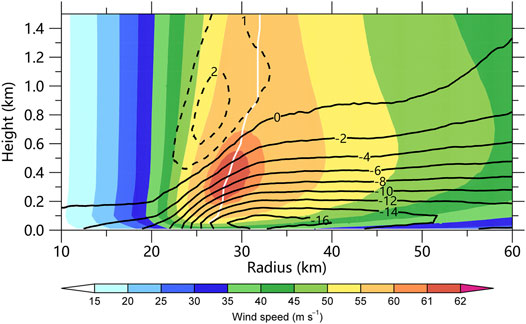
FIGURE 1. The radius–height cross section of the azimuthal mean tangential wind (shading, ms⁻¹) and radial wind (contour, ms⁻¹) of the simulated tropical cyclone, which were averaged over 26–36 h. The white line depicts the RMW.

Two types of wind profiles are derived from the 22-min wind data at 3-s intervals. The first kind of profiles is simultaneously collected in a vertical column of the wind field. To mimic the real GPS dropsonde profiles and make more direct comparison, we construct the second kind of dropsonde profiles by simulating the dropsonde falling in the simulation. The simulated dropsonde (SD) falls only in response to gravity and drag force from the wind, and the latter is given by Hane (1975), Hock and Franklin (1999), and Stern and Bryan (2018)

where $\overrightarrow{V_r}$ denotes the relative speed of dropsonde to the wind, $A_p$ is the area of the parachute, ${\mathrm{\rho }}_a$ is the density of surrounding air, and $C_{ds}$ is the drag coefficient of the dropsonde. Stern and Bryan (2018) noted that the horizontal velocity of the dropsonde is almost the same as the surrounding wind speed. Therefore, the wind drag is almost only in the vertical direction. Like the GPS dropsondes in the real TCs, the simulated dropsonde is released at the altitude of 6,000 m during the first 10 min of the simulated data. The horizontal locations and time are randomly selected in the eyewall (17.5–30 km). The drag force in Eq 4 is set to be the same as the weight of the dropsonde, leading to the dropsonde falling at the speed of the real GPS dropsonde. Then the dropsonde locations at various vertical levels can be obtained by integrating a trajectory model.

A total of 3,895 dropsondes are effectively constructed for high-wind conditions. Similar to the GPS dropsondes, the individual wind profiles are also categorized into five categories. The five high-wind groups correspond to MBW in the ranges of 20–29 ms⁻¹ (316 profiles), 30–39 ms⁻¹ (565 profiles), 40–49 ms⁻¹ (660 profiles), 50–59 ms⁻¹ (1,064 profiles), and 60–69 ms⁻¹ (1,290 profiles). The second type of wind profile is simultaneously collected in the vertical. Unlike the RD and SD profiles, the wind data at various altitudes are simultaneous and there are no horizontal drifts. The horizontal locations and time are also selected randomly. There are 7,151 wind profiles in high-wind conditions in the ranges of 20–29 ms⁻¹ (495 profiles), 30–39 ms⁻¹ (1,138 profiles), 40–49 ms⁻¹ (1,335 profiles), 50–59 ms⁻¹ (2,448 profiles), and 60–69 ms⁻¹ (1735 profiles). For convenience, we call the second type the idealized dropsonde (ID) profiles. The purpose of the ID profiles is to evaluate the sampling error in the SD wind profiles.

The Estimated Drag Coefficient

In this study, we linearly interpolate wind profile (horizontal component) with height onto every level that is 20 m apart and starts with 10 m. For the model output, the height is calculated from the geopotential height. For the observational data, the GPS height is used when estimating the altitude of the dropsonde. For simplicity, following Powell et al., 2003, we set the boundary layer to be 1200 m thick. Taking the categories of 20–29 ms⁻¹, 40–49 ms⁻¹, and 60–69 ms⁻¹ as an example, Figure 2 shows the mean horizontal wind and their variance of ID, SD, and RD from the same MBW bins. The fitting of the logarithmic linear regression is also plotted in Figure 2. Since the dropsondes data are known to be heavily contaminated at the 10-m level (Jarosz et al., 2007), they were not included in the regression. Figure 2 indicates that the simulated wind profiles (SD and ID) generally follow the log-profile, as shown in Figure 2A. The boundary layer jet in the model as shown in Figures 2B,C is lower than that observed, which is likely a result of the simulated TC being stronger than most TCs observed using dropsondes (Kepert and Wang, 2001).

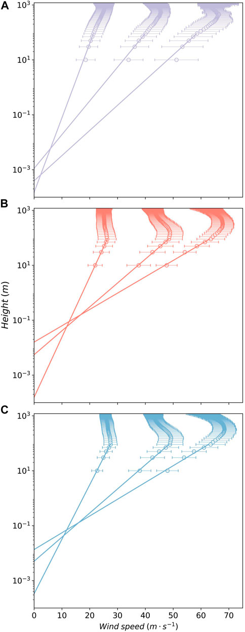
FIGURE 2. The RD (A), SD (B), and ID (C) wind profiles for the MBW categories of 20–29 ms⁻¹, 40–49 ms⁻¹, and 60–69 ms⁻¹. The line in (B) and (C) is regressed using wind from 10 to 100 m, while the lowest level in (A) was not used for regression.

The drag coefficient derived from the three types of wind profiles is shown in Figure 3. We used a bootstrap method to calculate the error bar. That is, a sampling with replacement of the same size as the dataset used was conducted. We calculated drag coefficients from each sample and used their 2.5 and 97.5% percentile as the boundaries of the 95% confidence interval. The drag coefficient based on the RD profile is between 1.0 × 10⁻³ and 2.0 × 10⁻³ and peaks for the category of 40–49 ms⁻¹. For comparison with the previous studies, note that horizontal coordinate is the wind speed at 10 m. The resulting drag coefficient agrees very well with the result in Powell et al. (2003).

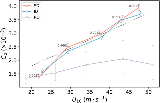
FIGURE 3. Drag coefficient derived from the RD (purple), SD (red), and ID (blue) wind profiles for the MBW categories of 20–29 ms⁻¹, 30–39 ms⁻¹, 40–49 ms⁻¹, 50–59 ms⁻¹, and 60–69 ms⁻¹. The error bar denotes the 95% confidence interval. The dot–dash line is an extrapolation based on Large and Pond (1981), which is applicable up to 25 ms⁻¹.

For the SD and ID profiles, as shown in Figure 3, the derived drag coefficient increases with the increasing MBW speed, although it is close to the drag coefficient of the RD for the category of 20–29 ms⁻¹. One may be wondering about the large spread of the derived drag coefficient from the RD profiles. One possible reason is that the RD profiles were from different TCs, while the SD and ID profiles are from the same TC. An important feature of the derived drag coefficient from the SD and ID profiles is that it increases linearly with the MBW or near-surface wind speed. For the category of 60–69 ms⁻¹, it can be as large as $4\times {10}^{-3}$, almost twice as much as the typical observation. It is interesting that the drag coefficient in the simulation is in good agreement with the extrapolated classic Large and Pond formula (Large and Pond, 1981). Note that the formula of Large and Pond (1981) is only valid for wind speed less than 25 ms⁻¹.

As mentioned above, the wind data of the SD profiles at various altitudes are not simultaneous and there are horizontal drifts. In addition, the sampling bias may be due to the boundary layer inflow or the presence of small-scale coherent structures, such as tornado-scale vortices and boundary layer rolls since the dropsondes can be repelled from strong updrafts in the boundary layer. For most of the MBW bins as shown in Figure 3, the differences in the drag coefficient between the SD and ID profiles can be 8% in the high-wind condition. Given the same MBW, the drag coefficient of the SD profiles has a smaller $u_{10}$ and larger $C_d$. It is suggested that the sampling bias has some influence on the derived drag coefficient, but the sampling bias has little influence on the increasing drag coefficient with the increase of the MBW speed.

Summary

In this study, based on the high-resolution simulation of the TC, the drag coefficient is calculated with the wind profile method (Powell et al., 2003). The numerical experiment was conducted over the open ocean using the WRF-LES model at the finest grid spacing of 37 m. While the simulated drag coefficient is similar to the observation in the category of 20–29 ms⁻¹, it does not show the leveling off or decrease in the strong wind conditions, likely due to the fact that in LES framework cannot take the complicated response from the sea surface, including sea foam, wave-breaking, and sheltering effect. For the strong wind conditions, the drag coefficient can be as large as $4\times {10}^{-3}$, almost twice as much as the typical observation. It is interesting that the drag coefficient in the simulation is in strong agreement with the extrapolated classic Large and Pond formula (Large and Pond, 1981). Since it has been demonstrated that the drag coefficient in high-wind condition does not increase linearly with surface wind speed (Powell et al., 2003), this study suggests that the boundary wind structure of the TC simulated with the LES technique may be unrealistic when the TC–ocean interaction is not fully considered.

Data Availability Statement

The raw data supporting the conclusions of this article will be made available by the authors, without undue reservation.

Author Contributions

LW conducted analysis and writing. WJ conducted analysis and writing. QL conducted the numerical experiment.

Conflict of Interest

The authors declare that the research was conducted in the absence of any commercial or financial relationships that could be construed as a potential conflict of interest.

Acknowledgments

The authors thank X. Qiu and W. Lin for many helpful discussions and advice. This study was jointly supported by the National Natural Science Foundation of China (41730961, 61827901, 41905001), and the scientific Research Program of Shanghai Municipal Science and Technology Commission (19dz1200101).

References

Bell, M. M., Montgomery, M. T., and Emanuel, K. A. (2012). Air-Sea Enthalpy and Momentum Exchange at Major Hurricane Wind Speeds Observed during CBLAST. J. Atmos. Sci. 69 (11), 3197–3222. doi:10.1175/JAS-D-11-0276.1
Cécé, R., Bernard, D., Krien, Y., Leone, F., Candela, T., Péroche, M., et al. (2021). A 30 M Scale Modeling of Extreme Gusts during Hurricane Irma (2017) Landfall on Very Small Mountainous Islands in the Lesser Antilles. Nat. Hazards Earth Syst. Sci. 21 (1), 129–145. doi:10.5194/nhess-21-129-2021
Donelan, M. A., Haus, B. K., Reul, N., Plant, W. J., Stiassnie, M., Graber, H. C., et al. (2004). On the Limiting Aerodynamic Roughness of the Ocean in Very Strong Winds. Geophys. Res. Lett. 31 (18). doi:10.1029/2004GL019460
Donelan, M. A. (2018). On the Decrease of the Oceanic Drag Coefficient in High Winds. J. Geophys. Res. Oceans. 123 (2), 1485–1501. doi:10.1002/2017JC013394
Edson, J. B., Jampana, V., Weller, R. A., Bigorre, S. P., Plueddemann, A. J., Fairall, C. W., et al. (2013). On the Exchange of Momentum over the Open Ocean. J. Phys. Oceanogr. 43 (8), 1589–1610. doi:10.1175/JPO-D-12-0173.1
French, J. R., Drennan, W. M., Zhang, J. A., and Black, P. G. (2007). Turbulent Fluxes in the Hurricane Boundary Layer. Part I: Momentum Flux. J. Atmos. Sci. 64 (4), 1089–1102. doi:10.1175/JAS3887.1
Green, B. W., and Zhang, F. (2015). Numerical Simulations of Hurricane Katrina (2005) in the Turbulent Gray Zone. J. Adv. Model. Earth Syst. 7, 142–161. doi:10.1002/2014MS000399
Hane, C. E. (1975). The Trajectories of Dropsondes in Simulated Thunderstorm Circulations. Mon. Weather Rev. 103 (8), 709–716. doi:10.1175/1520-0493(1975)103<0709:TTODIS>2.0.CO;2
Hock, T. F., and Franklin, J. L. (1999). The NCAR GPS Dropwindsonde. Bull. Am. Meteorol. Soc. 80 (3), 407–420. doi:10.1175/1520-0477(1999)080<0407:TNGD>2.0.CO;2
Ito, J., Oizumi, T., and Niino, H. (2017). Near-surface Coherent Structures Explored by Large Eddy Simulation of Entire Tropical Cyclones. Sci. Rep. 7 (1), 3798. doi:10.1038/s41598-017-03848-w
Jarosz, E., Mitchell, D. A., Wang, D. W., and Teague, W. J. (2007). Bottom-Up Determination of Air-Sea Momentum Exchange under a Major Tropical Cyclone. Science. 315 (5819), 1707–1709. doi:10.1126/science.1136466
Jiang, Y., Wu, L., Zhao, H., Zhou, X., and Liu, Q. (2020). Azimuthal Variations of the Convective-Scale Structure in a Simulated Tropical Cyclone Principal Rainband. Adv. Atmos. Sci. 37 (11), 1239–1255. doi:10.1007/s00376-020-9248-x
Kepert, J., and Wang, Y. (2001). The Dynamics of Boundary Layer Jets within the Tropical Cyclone Core. Part II: Nonlinear Enhancement. J. Atmos. Sci. 58 (17), 2485–2501. doi:10.1175/1520-0469(2001)058<2485:TDOBLJ>2.0.CO;2
Large, W. G., and Pond, S. (1981). Open Ocean Momentum Flux Measurements in Moderate to Strong Winds. J. Phys. Oceanogr. 11 (3), 324–336. doi:10.1175/1520-0485(1981)011<0324:OOMFMI>2.0.CO;2
Mirocha, J. D., Lundquist, J. K., and Kosović, B. (2010). Implementation of a Nonlinear Subfilter Turbulence Stress Model for Large-Eddy Simulation in the Advanced Research WRF Model. Mon. Weather Rev. 138 (11), 4212–4228. doi:10.1175/2010MWR3286.1
Powell, M. D., Vickery, P. J., and Reinhold, T. A. (2003). Reduced Drag Coefficient for High Wind Speeds in Tropical Cyclones. Nature. 422 (6929), 279–283. doi:10.1038/nature01481
Ren, Y., Zhang, J. A., Vigh, J. L., Zhu, P., Liu, H., Wang, X., et al. (2020). An Observational Study of the Symmetric Boundary Layer Structure and Tropical Cyclone Intensity. Atmosphere. 11 (2), 158. doi:10.3390/atmos11020158
Rotunno, R., Chen, Y., Wang, W., Davis, C., Dudhia, J., and Holland, G. J. (2009). Large-Eddy Simulation of an Idealized Tropical Cyclone. Bull. Amer. Meteorol. Soc. 90 (12), 1783–1788. doi:10.1175/2009bams2884.1
Stern, D. P., and Bryan, G. H. (2018). Using Simulated Dropsondes to Understand Extreme Updrafts and Wind Speeds in Tropical Cyclones. Mon. Weather Rev. 146 (11), 3901–3925. doi:10.1175/MWR-D-18-0041.1
Vickery, P. J., Wadhera, D., Powell, M. D., and Chen, Y. (2009). A Hurricane Boundary Layer and Wind Field Model for Use in Engineering Applications. J. Appl. Meteorol. Climatol. 48 (2), 381–405. doi:10.1175/2008JAMC1841.1
Wang, J., Young, K., Hock, T., Lauritsen, D., Behringer, D., Black, M., et al. (2015). A Long-Term, High-Quality, High-Vertical-Resolution GPS Dropsonde Dataset for Hurricane and Other Studies. Bull. Am. Meteorol. Soc. 96 (6), 961–973. doi:10.1175/BAMS-D-13-00203.1
Wu, L., Liu, Q., and Li, Y. (2018). Prevalence of Tornado-Scale Vortices in the Tropical Cyclone Eyewall. Proc. Natl. Acad. Sci. USA. 115 (33), 8307–8310. doi:10.1073/pnas.1807217115
Wu, L., Liu, Q., and Li, Y. (2019). Tornado-scale Vortices in the Tropical Cyclone Boundary Layer: Numerical Simulation with the WRF-LES Framework. Atmos. Chem. Phys. 19, 2477–2487. doi:10.5194/acp-19-2477-2019
Zhang, J. A., Rogers, R. F., Nolan, D. S., and Marks, F. D. (2011). On the Characteristic Height Scales of the Hurricane Boundary Layer. Mon. Weather Rev. 139 (8), 2523–2535. doi:10.1175/MWR-D-10-05017.1
Zheng, Y., Wu, L., Zhao, H., Zhou, X., and Liu, Q. (2020). Simulation of Extreme Updrafts in the Tropical Cyclone Eyewall. Adv. Atmos. Sci. 37 (7), 781–792. doi:10.1007/s00376-020-9197-4
Zhou, X., Wu, L., Liu, Q., and Zheng, Y. (2020). Influence of Low-Level, High-Entropy Air in the Eye on Tropical Cyclone Intensity: A Trajectory Analysis. J. Meteorol. Soc. Jpn. 98, 1231–1243. doi:10.2151/jmsj.2020-063
Zhu, P. (2008). Simulation and Parameterization of the Turbulent Transport in the Hurricane Boundary Layer by Large Eddies. J. Geophys. Res. 113, D17104. doi:10.1029/2007JD009643
Keywords: drag coefficient, tropical cyclone, numerical simulation, large-eddy simulation, air–sea interaction
Citation: Jiang W, Wu L and Liu Q (2021) High-Wind Drag Coefficient Based on the Tropical Cyclone Simulated With the WRF-LES Framework. Front. Earth Sci. 9:694314. doi: 10.3389/feart.2021.694314
Received: 12 April 2021; Accepted: 05 May 2021;
Published: 20 May 2021.
Edited by:
Qingqing Li, Nanjing University of Information Science and Technology, ChinaReviewed by:
Zhanhong Ma, National University of Defense Technology, ChinaJie Tang, China Meteorological Administration, China
Copyright © 2021 Jiang, Wu and Liu. This is an open-access article distributed under the terms of the Creative Commons Attribution License (CC BY). The use, distribution or reproduction in other forums is permitted, provided the original author(s) and the copyright owner(s) are credited and that the original publication in this journal is cited, in accordance with accepted academic practice. No use, distribution or reproduction is permitted which does not comply with these terms.
*Correspondence: Liguang Wu, liguangwu@fudan.edu.cn