


1. Introduction
The origins of the analysis of small amplitude unsteady disturbances (in the free-stream velocity) on a flat-plate boundary layer can be traced back to Lighthill (Reference Lighthill1954), in which the far-downstream, two-dimensional flow was analysed, showing that a double structure forms, with an inner classical Stokes layer, determined locally. In addition to these, what are effectively, inhomogeneous solutions, far-downstream eigensolutions also exist, and these form the nub of the present paper (but with particular emphasis on three-dimensional disturbances). Lam & Rott (Reference Lam and Rott1960) described such a family of unsteady eigensolutions, located close to the surface of a flat plate, which all decay exponentially fast downstream, and with shortening wavelength, with the eigenvalues being determined by the zeros of the derivative of the Airy function,  $\mbox {Ai}^\prime (z)$. The development of matched asymptotic methods subsequently enabled Ackerberg & Phillips (Reference Ackerberg and Phillips1972) and Lam & Rott (Reference Lam and Rott1993) to describe the nature of the associated eigenfunctions in a rather more formal manner. The importance of this family of eigensolutions was highlighted by Goldstein (Reference Goldstein1983), who showed that the first (and in fact fastest decaying) member of this family eventually becomes an Orr–Sommerfeld mode, which in turn leads to a growing disturbance downstream – an interesting example of boundary-layer receptivity (see also Goldstein, Sockol & Sanz Reference Goldstein, Sockol and Sanz1983; Hammerton & Kerschen Reference Hammerton and Kerschen1996). In parallel to this aforementioned family of eigenmodes, Brown & Stewartson (Reference Brown and Stewartson1973) described an alternative, and seemingly disparate family of unsteady eigenmodes, focused on the outer edge of a boundary layer, with a wavespeed close to that of the free-stream velocity. The asymptotic structure for the disturbances comprises three regions. The resulting eigenvalues were determined from matching the solutions in the two outer regions, with the inner-most region playing a relatively passive role. The eigenvalues were given in terms of the zeros of the Airy function,
  $\textrm {Ai}(z)$, with all disturbances decaying exponentially fast downstream. This latter work is technically quite challenging, and is a fine example of early matched asymptotic analysis. In spite of the clear physical significance of the Lam & Rott (Reference Lam and Rott1960) family, there is (in the words of Hammerton Reference Hammerton1999) an unappealing feature of these eigenmodes, insofar as they are inversely ordered downstream, with the leading-order modes decaying faster than the higher-order modes. On the other hand, the Brown & Stewartson (Reference Brown and Stewartson1973) family are well ordered, as the higher-order modes decay faster downstream, although this family has received somewhat less attention than the ‘competing’ family.
A number of attempts have been made to reconcile the two families from the numerical solutions of the linearised unsteady boundary-layer equations. Hammerton (Reference Hammerton1999) made a comparison of these two asymptotic eigensolutions. He was able to identify both these modes in his accompanying numerical solutions by (a rather ingenious) consideration of the analytic continuation into the complex streamwise ( $x$)-plane of both sets of eigensolutions. The decay rate of each mode was observed and the different locations of the dominant disturbance eigenfunctions in the boundary layer were described.
Needless to say, the important engineering implications of boundary-layer transition have attracted enormous interest over the years, including experimental, computational and theoretical studies. Although there has been a good understanding of Tollmien–Schlichting waves in general (in the early stages of boundary-layer instability/transition), and these are well documented, an understanding of the later stages of these processes (especially of a three-dimensional nature) is still attracting much attention. Pertinent studies include Leib, Wundrow & Goldstein (Reference Leib, Wundrow and Goldstein1999), Ricco & Wu (Reference Ricco and Wu2007), Ricco (Reference Ricco2009) and Kátai & Wu (Reference Kátai and Wu2020) for example. These papers include a comprehensive list and review of previous work, especially in the three-dimensional context. The trigger for a lot of interest can be traced back to the experimental work of Klebanoff (Reference Klebanoff1971), in which free-stream turbulence was seen to trigger responses in a boundary layer of a much smaller frequency than that of Tollmien–Schlichting waves. The associated spanwise scales of the resulting perturbations are quite narrow.
In this paper, unlike some of the more recent work (which is mostly driven by problems involving receptivity), our emphasis is mostly (but not exclusively) on homogeneous flow structures, that persist far downstream of triggering mechanisms (indeed, this is in the spirit of the aforementioned papers of Ackerberg & Phillips (Reference Ackerberg and Phillips1972), Lam & Rott (Reference Lam and Rott1960) and Brown & Stewartson (Reference Brown and Stewartson1973).
In § 2 we present the over-arching methodology for the paper, namely the boundary-region equations, in which the spanwise length scales are generally comparable to the boundary-layer thickness. In § 3 we present numerical results for the downstream development of small amplitude, specified spanwise wavelength disturbances imposed on a Blasius boundary layer. These results indicate that downstream growth is a real possibility (in contrast to what is observed for fully two-dimensional disturbances). In the following § 4, a locally parallel investigation is mounted for eigensolutions, at selected downstream locations, an approach that is clearly heuristic, but one that does become valid further downstream. This approach confirms the possible existence of downstream-growing, three-dimensional disturbances, in particular linked to the first (leading-order) Lam & Rott (Reference Lam and Rott1960)/Ackerberg & Phillips (Reference Ackerberg and Phillips1972) mode. Section 5 considers an asymptotically rigorous approach, valid far downstream, to the eigenproblem, and is able to confirm conclusively, a number of the key points highlighted in § 4, including the all important potential for downstream growth. Section 6 focuses on the three-dimensional analogy to the Brown & Stewartson (Reference Brown and Stewartson1973) modes, and clearly illustrates the stabilising nature of increasing spanwise wavenumber for this family (a feature clearly observed using the approach of § 4). Some conclusions are presented in § 7.
2. Methodology (the boundary-region equations)
We consider the three-dimensionally disturbed and temporally harmonic flow over a semi-infinite plate, where the spanwise scale is generally comparable to the boundary-layer thickness. We define a Reynolds number  $Re={U_\infty L}/{\nu }$, which is taken to be asymptotically large, where
  $U_\infty$ is a free-stream (reference) flow speed,
  $L$ is some reference length scale and
  $\nu$ the kinematic viscosity, assumed to be constant (consistent with an incompressible fluid). We write the velocity vector (to leading order in powers of Reynolds number) as
  $U_\infty (U,Re^{-1/2 }V,Re^{-1/2 }W)$, corresponding to the coordinates
  $L(x, Re^{-1/2 } Y, Re^{-1/2 } Z)$, where the plate lies along
  $Y=0$,
  $x>0$. Correspondingly, the pressure takes the form
  $\rho U_\infty ^2 (p_0+Re^{-1/2 } p_1(x)+ Re^{-1} p_2(x,Y,Z,t)+\ldots )$, where
  $\rho$ is the fluid density, dimensional time is
  ${L t}/{U_\infty }$, and we are implicitly assuming a uniform free-stream flow, and so we can assume that
  $p_0^{\prime }=0$. (It should be noted, however, that the underlying methodology could be extended to more general classes of free stream, provided streamwise variations
  $p_0^{\prime }=O(1)$, with little adaptation.) Regarding
  $p_{1}(x)$, this is caused by the displacement effect of the Blasius boundary layer, and is not necessarily zero (see Van Dyke Reference Van Dyke1994), but does not play a role in our analysis. The resulting equations are well established (see Rubin Reference Rubin1966; Goldstein et al. Reference Goldstein, Sescu, Duck and Choudhari2016; Hewitt & Duck Reference Hewitt and Duck2018, Reference Hewitt and Duck2019) and are generally referred to as the boundary-region equations following the terminology of Kemp (Reference Kemp1951); these take the form
 \begin{gather} U_x + V_Y + W_Z=0, \end{gather}
 \begin{gather}U_t+UU_x+VU_Y+WU_Z= U_{YY}+ U_{ZZ}, \end{gather}
 \begin{gather}V_t+UV_x+VV_Y+WV_Z+p_{2Y}= V_{YY}+V_{ZZ}, \end{gather}
 \begin{gather}W_t+UW_x+VW_Y+WW_Z+p_{2Z}=W_{YY}+W_{ZZ}. \end{gather}
This system is (asymptotically) rigorous to leading order in powers of Reynolds number.
We now decompose the solution into an undisturbed (Blasius) state and a small amplitude, unsteady (harmonic) perturbation, periodic in the spanwise direction, namely as follows:
 \begin{gather} U=U_B(\eta)+\epsilon \,\mathrm{e}^{\mathrm{i}t} u(x,\eta) \cos \mu Z +\ldots, \end{gather}
 \begin{gather}V=x^{{-}1/2 } (V_B(\eta) +\epsilon \,\mathrm{e}^{\mathrm{i}t} v(x,\eta) \cos \mu Z) +\ldots, \end{gather}
 \begin{gather}W=\epsilon \,\mathrm{e}^{\mathrm{i}t} w(x,\eta) \sin \mu Z +\ldots, \end{gather}
where the flow perturbation amplitude  $|\epsilon | \ll 1$ (leading to a linear system for the flow perturbation), whilst
  $\eta =Y/\sqrt {x}$ in line with the undisturbed Blasius form, viz.
 \begin{gather} {-}\tfrac{1}{2}\eta U^{\prime}_{B}+V_{B}^{\prime}=0, \end{gather}
 \begin{gather} {-}\tfrac{1}{2}\eta U_{B}^{\prime} U_B + V_B U^{\prime}_{B} =U_{B}^{\prime\prime}. \end{gather}
In (2.5)–(2.7) without loss of generality, we have set the temporal frequency parameter to unity, and complex conjugates are assumed.
For the purposes of § 6, it is useful to introduce what is effectively a similarity streamfunction  $f(\eta )$, where
  $U_B=f'(\eta )$ and
  $V_B =\tfrac 12(\eta f'-f)$, and
  $f$ satisfies
 \begin{equation} f'''+\tfrac{1}{2}ff''=0, \end{equation}
subject to the boundary conditions  $f(0)=f'(0)=0$ and
  $f'(\eta )\to 1$ as
  $\eta \to \infty$.
At this point, we define a (perturbation) streamwise component of vorticity,  $\varTheta = W_Y-V_Z$ as follows:
 \begin{equation} \varTheta = \epsilon x^{{-}1/2 } \,\mathrm{e}^{\mathrm{i} t} \theta (x,\eta) \sin \mu Z +\ldots, \end{equation}
which is useful if, as we do, we eliminate  $p_2$ between the transverse and spanwise momentum equations. This is very convenient for the subsequent numerical analysis. The net result for the perturbation quantities is as follows:
 \begin{gather} x u_x -\tfrac12 \eta u_\eta+ v_\eta+x \mu w =0, \end{gather}
 \begin{gather}\theta=w_\eta+\mu v, \end{gather}
 \begin{gather}\mathrm{i} x u +U_B(-\tfrac12 \eta u_\eta +x u_x) -\tfrac12 \eta u U_{B}^{\prime} + v U_{B}^{\prime}+V_B u_\eta-u_{\eta\eta}+x \mu^2 u=0,\end{gather}
 \begin{gather} - \mathrm{i} x \theta+U_B(\tfrac12 \theta+\tfrac12 \eta \theta_\eta -x\theta_x)-V_B\theta_\eta-V_{B}^{\prime}\theta +\tfrac12 x\mu u (V_B+\eta V_{B}^{\prime})\nonumber\\ \hspace{-2.8pc}+ \ U_{B}^{\prime}(-\tfrac12 \eta w_\eta+xw_x)+\theta_{\eta\eta}-x \mu^2 \theta=0. \end{gather}
The above system of equations then forms the backbone to this paper.
3. Downstream development of unsteady perturbations
We first consider fully numerical solutions to the system (2.12)–(2.15). Clearly, for two-dimensional perturbations  $\mu =0$, and the system far downstream mirrors that of Ackerberg & Phillips (Reference Ackerberg and Phillips1972), Lam & Rott (Reference Lam and Rott1960) and indeed Brown & Stewartson (Reference Brown and Stewartson1973) with eigensolutions which are well known to decay. This system was solved using a standard, second-order, parabolic marching scheme. Disturbances were triggered by forcing the perturbation close to the leading edge,
  $x=0$. Generally, this was performed by the following forcing:
 \begin{equation} w(x,\eta=0)=\mathrm{e}^{{-}1/x^2} \,\mathrm{e}^{{-}x^2}, \end{equation}
thereby mimicking a short impulse at the start of the computation. This confirmed the downstream decay when  $\mu =0$, albeit with diminishing streamwise length scale oscillations, in line with the results of Ackerberg & Phillips (Reference Ackerberg and Phillips1972) and Lam & Rott (Reference Lam and Rott1960). However, as
  $\mu$ was increased, the decay was no longer uniformly apparent, even for very modest values of spanwise wavenumber
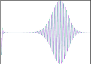
  $\mu$. Figure 1 shows results corresponding to the spanwise vorticity on the plate surface
  $\theta (x,\eta =0)$ for
  $\mu =0.05$,
  $0.04$,
  $0.03$,
  $0.02$. These indicate a clear transition from what appears to be a generally uniformly downstream decaying state, through to a regime in which disturbances grow (this can be quite significant), followed by decay. This change in behaviour appears to be between
  $\mu =0.03$ (which exhibits growth) and
  $\mu =0.04$ (which exhibits general decay). Further, perhaps more startling, evidence for downstream growth (followed by eventual decay) is presented in figure 2, for the behaviour of
  $\log |\theta (x,\eta =0)|$ for
  $\mu =0.005$,
  $0.01$ and
  $0.02$. For the smallest of these values, very significant downstream growth occurs (which, in reality, would be way outside of any linearly relevant regime). This behaviour is in stark contrast to the two-dimensional results which as noted above all decay downstream – just small amounts of three-dimensionality can provoke a significant change in flow characteristics. To better understand this apparent dichotomy, in the following section we mount a local stability analysis (which also sheds some light on the relationship between the two ‘competing’ families of two-dimensional modes).

Figure 1. Downstream development of  $\theta (x,\eta =0)$.

Figure 2. Downstream development of  $\log |\theta (x,\eta =0)|$.
4. Local eigenmode/stability analysis
To better comprehend the mismatch between the well-known two-dimensional results (corresponding to  $\mu =0$) and the growth (in some cases very significant growth) downstream for very small values of the spanwise wavenumber, the next step is to perform a (heuristic) local stability analysis, at finite values of the downstream location
  $x$. For this, we write
 \begin{equation} (u,v,w,\theta)=(u^*(\eta),v^*(\eta),w^*(\eta),\theta^*(\eta))\,\mathrm{e}^{\nu x}, \end{equation}
where  $\nu$ is in effect an eigenvalue, indicating growth if
  $\textrm {Re}\{\nu \}>0$ and decay if
  $\textrm {Re}\{\nu \}<0$. Substitution into (2.12)–(2.15) leads to the following homogeneous system:
 \begin{gather} x \nu u^* -\tfrac12 \eta u^{*\prime}+ v^{*\prime}+x \mu w^* =0, \end{gather}
 \begin{gather}\theta^*=w^{*\prime}+\mu v^*, \end{gather}
 \begin{gather}\mathrm{i} x u^{*} +U_B(-\tfrac12 \eta u^{*\prime} +x \nu u^{*}) -\tfrac12 \eta u^{*} U_{B}^{\prime} + v^{*} U_{B}^{\prime}+V_B u^{*\prime}-u^{*\prime\prime}+x \mu^2 u^{*}=0,\end{gather}
 \begin{gather} - \mathrm{i} x \theta^*+U_B(\tfrac12 \theta^*+\tfrac12 \eta \theta^{*\prime} -x\nu\theta^*)-V_B\theta^{*\prime} -V_{B}^{\prime}\theta^* +\tfrac12 x\mu u^* (V_B+\eta V_{B}^{\prime})\nonumber\\ \hspace{-3.3pc} + \ U_{B}^{\prime}(-\tfrac12 \eta w^{*\prime}+x\nu w^*)+\theta^{*\prime\prime} -x \mu^2 \theta^*=0. \end{gather}
 The eigenvalues  $\nu$ to this system were evaluated using a straightforward finite-difference scheme, combined with (in the first instance) a QZ routine and then (if necessary, to confirm numerical accuracy) a local Newton search routine (using the aforementioned QZ values as initial estimates). Let us first consider the case
  $\mu =0$. Figure 3 presents results at three downstream locations, namely
  $x=25$,
  $50$ and
  $100$. The first Ackerberg & Phillips (Reference Ackerberg and Phillips1972)/Lam & Rott (Reference Lam and Rott1960) modes are identified as 2Di, 2Dii, 2Diii, and as expected have
  $\arg \{\nu \}\approx -3{\rm \pi} /4$ (further details regarding these modes will be described in the following section). However, additional (three-dimensional) modes also exist, where
  $w^*\ne 0$, identified as 3Di, 3Dii, 3Diii, and these too exhibit the property
  $\arg \{\nu \}\approx -3{\rm \pi} /4$. Details regarding these will (also) be described in the following section, and in fact are similar to those reported by Ricco & Wu (Reference Ricco and Wu2007), where the emphasis in this latter paper was the modes connected to those of Ackerberg & Phillips (Reference Ackerberg and Phillips1972)/Lam & Rott (Reference Lam and Rott1960) (and also on the compressible regime).

Figure 3. Distributions of eigenvalues  $\nu$ at selected downstream locations (
 $\mu =0$).
There are several key observations to be gleaned from the results in figure 3:
(i) At finite
 $x$ downstream locations, only a finite number of modes with $\arg \{\nu \}\approx -3{\rm \pi} /4$ are clearly identifiable, but the number of these increases further downstream.
(ii) There appear to be many eigenvalues, quite distinct from those above, with
$-\textrm {Im}\{\nu \}$ values of close to unity; the indications are therefore that these correspond to the Brown & Stewartson (Reference Brown and Stewartson1973) modes, with a wavespeed close to that of the free stream.(iii) The
$\arg \{\nu \}\approx -3{\rm \pi} /4$ modes appear to be spawned from the Brown & Stewartson (Reference Brown and Stewartson1973) modes, the higher modes appearing at progressively further downstream locations.(iv) The amplitude
$|\nu |$ of a given $\arg \{\nu \}\approx -3{\rm \pi} /4$ mode increases downstream; this is partly to be expected from Ackerberg & Phillips (Reference Ackerberg and Phillips1972) and Lam & Rott (Reference Lam and Rott1960) (and see also the analysis in the following section), but note the following point.(v) Inspection of the eigenmodes reveals that (even) for this choice of
$\mu =0$, in addition to the expected $w^* \equiv 0$ family, another family with $w^* \ne 0$, $u^*=v^* \equiv 0$ also exists; of necessity, continuity demands this degenerate form is possible only if $\mu =0$ (precisely).


Item (iii) above therefore gives some numerical evidence of a linkage between the two, previously reported, families of eigenvalues.
Let us now consider the effect of  $\mu \ne 0$; figure 4 shows results for modes 2Di and 3Di, for increasing
  $\mu$ at
  $x=50$. What is particularly noteworthy with figure 4 is that
  $\textrm {Re}\{\nu \}$ exhibits a region of positive values (identifiable where
  $\textrm {Re}\{\nu \}>0$), suggesting downstream growth of disturbances linked to mode 2Di – the first Ackerberg & Phillips (Reference Ackerberg and Phillips1972)/Lam & Rott (Reference Lam and Rott1960) mode. This appears to be a quite significant observation, and this does provide an explanation for the downstream growth behaviour found in the marching procedure results described in the previous section. It should be noted that the behaviour of mode 3Di seems quite benign (in comparison), and no other (two- or three-dimensional) modes appear to display regions of growth. In the following section we perform asymptotic analyses that further demonstrate (and confirm) this behaviour. We also find that the eigenvalues described in (ii) above persist in the same manner for
  $\mu \ne 0$. The asymptotic analysis in § 6 describes this family of eigensolutions.

Figure 4. Eigenvalue distributions for  $x=50$, increasing
  $\mu$.
5. The asymptotics of the far-downstream limit ($x \to \infty$)

Here, we focus on the effect of three-dimensionality on the Ackerberg & Phillips (Reference Ackerberg and Phillips1972)/Lam & Rott (Reference Lam and Rott1960) modes, an investigation suggested by the preceding sections. In other calculations, allied to those of figure 4, some of which will be presented later in this section, it was found that with increasing  $x$ (downstream location), the region for which
  $\textrm {Re}\{\nu \}>0$ occurs progressively close to
  $\mu =0$, but also
  $\max \{\textrm {Re}\{\nu \}\}$ increases. We start by following the (two-dimensional) procedure adopted by Ackerberg & Phillips (Reference Ackerberg and Phillips1972) and Lam & Rott (Reference Lam and Rott1960), but with the added proviso (in line with our previous comment) that the spanwise wavenumber
  $\mu$ must be small, specifically by assuming that
  $\hat {\mu }=x\mu =O(1)$ (an assertion that can be verified a posteriori). We also introduce
  $\lambda = -2 x^{-1/2} \nu /3$. This is consistent with previous literature, for which generally
  $\lambda =O(1)$, and indeed the (square-root) growth downstream of
  $|\nu |$ of these eigenmodes can be witnessed in figure 3.
We therefore expect that for  $x\gg 1$ the
  $Y=O(1)$ region is important. For the following analysis, we set
  $u^{*\prime }(\eta =0)=1$ (this is arbitrary, but practically any normalisation is permissible) then, for
  $Y=O(1)$, the leading-order terms take on the following form (note that algebraic terms of the form
  $x^{\tau }$ multiply the exponential terms below, as described by Goldstein (Reference Goldstein1983) and Hammerton & Kerschen (Reference Hammerton and Kerschen1996), but these are only necessary at higher order, beyond that considered in this paper, and are omitted in the interests of brevity)
 \begin{gather} U=\frac{U_B^{\prime}(0) Y}{\sqrt{x}} +\epsilon x^{{-}1/2 } \,\mathrm{e}^{\mathrm{i} t} \, \mathrm{e}^{-\lambda x^{3/2 }}\hat{u}(Y)\cos \frac{\hat \mu Z}{x} , \end{gather}
 \begin{gather}V=\frac{U_B^{\prime}(0)Y^2}{2x^{3/2 }} +\epsilon \,\mathrm{e}^{\mathrm{i} t} \,\mathrm{e}^{-\lambda x^{3/2 }} \hat{v}(Y) \cos \frac{\hat{\mu} Z}{x} , \end{gather}
 \begin{gather}p_2=\epsilon x^2 \,\mathrm{e}^{\mathrm{i} t} \,\mathrm{e}^{-\lambda x^{3/2 }} \hat{p}_2(Y) \cos \frac{\hat{\mu}Z}{x} , \end{gather}
 \begin{gather}W=\epsilon x \,\mathrm{e}^{\mathrm{i} t} \,\mathrm{e}^{-\lambda x^{3/2 }} \hat{w}(Y)\sin \frac{\hat{\mu}Z}{x} , \end{gather}
which leads to the following system of equations as  $x \to \infty$:
 \begin{gather} {-}\tfrac32 \lambda \hat{u} +\hat{v}^{\prime}+\hat{\mu}\hat{w}=0, \end{gather}
 \begin{gather}\mathrm{i} \hat{u} -\tfrac32 Y U_B^{\prime}(0) \lambda \hat{u} + U_B^{\prime}(0) \hat{v} - \hat{u}^{\prime\prime}=0, \end{gather}
 \begin{gather}\hat p_{2}^{\prime}=0, \end{gather}
 \begin{gather}\mathrm{i} \hat{w}-\tfrac32 \lambda Y U_B^{\prime}(0)\hat{w} - \hat{\mu}\hat{p}_{2}-\hat{w}^{\prime\prime}=0. \end{gather}
 Using continuity to eliminate  $\hat {v}^{\prime }$ in the streamwise momentum equation differentiated with respect to
  $Y$ leads to
 \begin{equation} \mathrm{i} \hat{u}^{\prime} -\tfrac32 Y U_B^{\prime}(0) \lambda \hat{u}^{\prime} -\hat{u}^{\prime\prime\prime} -\hat{\mu}\hat{w} U_B^{\prime}(0)=0. \end{equation}
Note that as  $Y \to \infty$, we require
 \begin{equation} \hat{u}, \quad \hat{w}=O(1), \quad \textrm{{whilst}} \ \hat{v}=O(Y). \end{equation}
Setting  $\hat {\mu }=0$ in the above, leads to the Ackerberg & Phillips (Reference Ackerberg and Phillips1972)/Lam & Rott (Reference Lam and Rott1960) system, and the solution of which can be written in terms of Airy functions, leading to the following estimates for the eigenvalues
  $\lambda$:
 \begin{equation} \lambda_n=\frac{\sqrt{2}(1+\mathrm{i})}{3 {(\rho_n^{\prime})}^{3/2} U_B^\prime(0)}, \end{equation}
where  $U_B^\prime (0)=0.332\ldots\,$ and
  $\rho ^{\prime }_n$ corresponds to the
  $n\textrm {th}$ (negative) zero of the derivative of the Airy function, viz.
 \begin{equation} \textrm{Ai}^{\prime}(-\rho_n^{\prime})=0. \end{equation}
This leads to  $\lambda =(1.380\ldots\,$,
  $0.242\ldots\,$,
  $0.134\ldots\,$,
  $\ldots\,$)
 $(1+\mathrm {i})$. These modes are denoted by 2Di, 2Dii, etc. in the earlier figures.
However, there also exists a three-dimensional family of eigenmodes, related to those reported by Ricco & Wu (Reference Ricco and Wu2007), which can also be written in terms of Airy functions, but for which  $\hat {v} \equiv \hat {p}_2 \equiv 0$, and this family has the following eigenvalues
  $\lambda$:
 \begin{equation} \lambda_n=\frac{\sqrt{2}(1+\mathrm{i})}{3 \rho_n^{3/2 } U_B^\prime(0)}, \end{equation}
where  $\rho _n$ corresponds to the
  $n\textrm {th}$ (negative) zero of the Airy function itself, viz.
 \begin{equation} \textrm{Ai}(-\rho_n)=0, \quad n=1,2,3,\ldots. \end{equation}
This leads to  $\lambda =(0.397 \ldots\,$,
  $0.1715\ldots\,$,
  $0.109 \ldots\,$,
  $\ldots\,$)
 $(1+\mathrm {i})$. These modes are denoted by 3Di, 3Dii, etc. in the earlier figures, all of which exhibit eigenmodes that decay (exponentially) as
  $Y\to \infty$, consistent with the analogous observations of Ricco & Wu (Reference Ricco and Wu2007) regarding their three-dimensional modes.
However, in order to compute eigenvalues for  $\hat {\mu } \ne 0$ to (5.5), (5.8) and (5.9) a fully numerical approach is necessary, but also requires a further (closure) condition, obtained by consideration of other regions normal to the plate surface.
Let us consider now the regime  $\eta =Y/\sqrt {x}=O(1)$ (i.e. a more-extensive wall normal scale). We then expect that (to leading order)
 \begin{gather} U=U_B(\eta)+\epsilon x^{{-}1/2 } \,\mathrm{e}^{\mathrm{i} t} \,\mathrm{e}^{-\lambda x^{3/2 }}\tilde{u}(\eta)\cos \frac{\hat{\mu}Z}{x}, \end{gather}
 \begin{gather}V=x^{{-}1/2} V_B(\eta)+\epsilon x^{1/2 } \,\mathrm{e}^{\mathrm{i} t} \,\mathrm{e}^{-\lambda x^{3/2 }} \tilde{v} (\eta)\cos \frac{\hat{\mu} Z}{x} , \end{gather}
 \begin{gather}p_2=\epsilon x^2 \,\mathrm{e}^{\mathrm{i} t} \,\mathrm{e}^{-\lambda x^{3/2 }}\tilde{p}_2(\eta) \cos \frac{\hat{\mu} Z}{x}, \end{gather}
 \begin{gather}W=\epsilon x^{1/2 } \,\mathrm{e}^{\mathrm{i} t} \,\mathrm{e}^{-\lambda x^{3/2 }} \tilde{w}(\eta)\sin \frac{\hat{\mu} Z}{x}. \end{gather}
These lead to the following set of equations:
 \begin{gather} O(1): \quad -\tfrac32 \lambda \tilde{u} +\tilde{v}^{\prime}=0, \end{gather}
 \begin{gather}O(1): \quad -\tfrac32 \lambda U_B \tilde{u} + U_{B}^{\prime} \tilde{v}=0, \end{gather}
 \begin{gather}O(x^{3/2 }): \quad \tilde{p}_{2}^{\prime}=0, \end{gather}
 \begin{gather}O(x): \quad -\tfrac32 \lambda U_B \tilde{w} =\hat{\mu}\tilde{p}_2. \end{gather}
The solution of this system is
 \begin{gather} \tilde{u} = A U_{B}^{\prime}, \end{gather}
 \begin{gather}\tilde{v}=\tfrac32 \lambda A U_B(\eta), \end{gather}
 \begin{gather}\tilde{w}={-}\frac{2\hat{\mu} \tilde{p}_2}{3\lambda U_B(\eta)}, \end{gather}
which matches to (5.10), where  $A$ is a constant and where clearly
  $\tilde {p}_2$ is a constant across this region.
If we now consider the region where  $\eta \gg 1$ (alternatively this can be regarded as the region wherein
  $\eta =O(\sqrt {x})$) then it is straightforward to see that the
  $V$ and
  $W$ perturbations are linked through the Cauchy–Riemann equations to yield
 \begin{gather} U=1+o(\epsilon \sqrt{x} \,\mathrm{e}^{-\lambda x^{3/2 }}) +\ldots , \end{gather}
 \begin{gather}V= x^{{-}1/2} V_B(\infty)+\epsilon x^{1/2 } C \,\mathrm{e}^{\mathrm{i} t} \,\mathrm{e}^{-\lambda x^{3/2 }} \,\mathrm{e}^{-{\eta\hat{\mu}}/{\sqrt{x}}}\cos \frac{\hat{\mu} Z}{x} +\ldots, \end{gather}
 \begin{gather}W=\epsilon x^{1/2 } C \,\mathrm{e}^{\mathrm{i} t} \,\mathrm{e}^{-\lambda x^{3/2 }}\,\mathrm{e}^{-{\eta\hat{\mu}}/{\sqrt{x}}} \sin \frac {\hat{\mu} Z}{x} +\ldots, \end{gather}
 \begin{gather}p_2={-}\frac{3\epsilon C}{2\hat{\mu}}\lambda x^2 \,\mathrm{e}^{\mathrm{i} t} \,\mathrm{e}^{-\lambda x^{3/2 }} \,\mathrm{e}^{-{\eta\hat{\mu}}/{\sqrt{x}}}\cos \frac{\hat{\mu} Z}{x} +\ldots. \end{gather}
 Here,  $C$ is a constant. The above implies that
 \begin{gather} C=\tfrac32 \lambda A, \end{gather}
 \begin{gather}\hat{w} (Y \to \infty) \to \frac{3 \lambda \hat{u}(Y \to \infty)}{2 (U_B'(0))^2 Y}, \end{gather}
and this (now) works as a key boundary condition, which closes the problem for (5.5), (5.8), (5.9). This is another eigenvalue problem, for which standard numerical (finite-difference) methods were employed.
In figure 5 we present results comparing these asymptotic behaviours for  $\textrm {Re}\{\lambda \}$ in the unstable regime, with (suitably scaled) results for increasing values of
  $x$; overall, the agreement is satisfactory.

Figure 5. The  $\textrm {Re}\{\lambda \}<0$ (unstable) region, for
  $x$ increasing, and compared to the asymptotic (
 $x \to \infty$) solution.
5.1. The limit of small wavelength, namely $\hat {\mu } \to \infty$

Even though the existence of an unstable (downstream-growing) regime is very clear, we are able to undertake further asymptotic analysis that leads to fully analytic evidence of this. The numerics strongly suggest that as  $\hat {\mu } \to \infty$
 \begin{equation} \lambda \to \mathrm{i}\hat{\mu}^{{-}1} \hat{\lambda}_0 +\hat{\mu}^{{-}2}\hat{\lambda}_1 +\ldots; \end{equation}
we can verify this analytically (in particular the imaginary nature of the leading-order term) a posteriori. Consider first  $Y=O(1)$, and now assume, consistent with earlier, the normalisation that
  $\hat {u}^{\prime }(Y=0)=1$. We focus our attention on
  $\hat {u}$,
  $\hat {w}$ and
  $\hat {p}_2$. We then expect that
 \begin{equation} (\hat{u}, \hat{w}, \hat{p}_2)=(u_0^*+\hat{\mu}^{{-}1}u_1^* ,\hat{\mu}^{{-}1} w_0^*+\hat{\mu}^{{-}2} w_1^*, \hat{\mu}^{{-}2} p_{20}^* +\hat{\mu}^{{-}3} p_{21}^*) +\ldots. \end{equation}
Immediately, (5.8) yields (ensuring the no-slip condition is satisfied)
 \begin{equation} w^*_0={-}\mathrm{i} p_{20}^* \left(1-\exp\left({-\frac{1+\mathrm{i}}{\sqrt{2} }Y}\right)\right). \end{equation}
Equation (5.9) then gives to leading order
 \begin{align} u_0^*={-}U_B^\prime(0)p_{20}^*Y\left( 1+\frac12 \exp\left({-\frac{1+\mathrm{i}}{\sqrt{2} }Y}\right) \right) +\frac{(1-\mathrm{i})p_{20}^*U_B^\prime(0)}{\sqrt{2}}\left(1-\exp\left({-\frac{1+\mathrm{i}}{\sqrt{2} }Y}\right)\right). \end{align}
From this, the behaviour as  $Y\to \infty$ is required, namely
 \begin{align} u^*_0 \to -{U_B^\prime(0) p_{20}^* Y} +\frac{1-\mathrm{i}}{\sqrt{2}} p_{20}^*U_B^\prime(0). \end{align}
Although in the above the diffusion terms have been retained, the eigenvalue ( $\hat {\lambda }_0$) term has not, but this will play a role when
  $\hat {Y}=Y/\hat {\mu } =O(1)$. On this further scale, to leading order we have
 \begin{equation} (\hat{u}, \hat{w})=(\hat{\mu} \bar{u}_0 +\bar{u}_1, \hat{\mu}^{{-}1} \bar{w}_0+\hat{\mu}^{{-}2} \bar{w}_1) +\ldots. \end{equation}
On this length scale, the diffusion terms are (generally) insignificant, yielding first
 \begin{gather} \bar{w}_0=\frac{2\mathrm{i} p_{20}^*}{3 \hat{\lambda}_0 U_B^\prime (0) \hat Y -2 }, \end{gather}
 \begin{gather}\bar{w}_1=\frac{2\mathrm{i} p_{21}^*+3\mathrm{i} \hat{\lambda}_1 \hat{Y} U_B^\prime(0) \bar{w}_0}{3 \hat{\lambda}_0 U_B^\prime (0) \hat{Y} -2 }, \end{gather}
and then (after satisfying matching with (5.36))
 \begin{gather} \bar{u}_0 = \frac{2 p_{20}^*}{3\hat{\lambda}_0}\left(1 -\frac{2}{2 -3 \hat{Y} \hat{\lambda}_0 U_B^\prime(0)} \right), \end{gather}
 \begin{gather} \hspace{-5pc}\bar{u}_1 = \frac{2 p_{21}^*}{3\hat{\lambda}_0}\left(1 -\frac{2}{2 -3 \hat{Y} \hat{\lambda}_0 U_B^\prime(0)} \right) +\frac{(1-\mathrm{i})p_{20}^* U_B^\prime(0)}{\sqrt{2}}\nonumber\\ \hspace{3.6pc} + \ \frac{4\mathrm{i} p_{20}^*\hat{\lambda}_1}{3 \hat{\lambda}_0^2}\left( -\frac{2}{2 -3\hat{\lambda}_0U_B^\prime (0)\hat Y} +\frac{2 }{\left(2 -3 \hat{\lambda}_0U_B^\prime (0)\hat{Y}\right)^2} +\frac12\right). \end{gather}
Finally, if we impose the condition (5.31), then to leading order in  $\hat {\mu }$
 \begin{equation} \hat {\lambda}_0 = \tfrac23 U_B^\prime (0), \end{equation}
thereby confirming our assertion that the leading-order term for  $\lambda$ is imaginary. The next order yields an estimate for
  $\hat {\lambda }_1$
 \begin{equation} \hat{\lambda}_1 ={-}\frac{9\hat{\lambda}_0^3(1+\mathrm{i})}{4\sqrt{2}}. \end{equation}
 Figure 5 shows results for  $\textrm {Re}\{\lambda \}$ obtained using (5.43), which can be compared to the previously described shown results in this figure, and in particular the comparison with the
  $x\to \infty$ results as
  $\hat {\mu }$ increases is excellent. It should be noted that, whereas the finite
  $x$ results appear to ‘stabilise’ for larger values of
  $\hat {\mu }$ (above a critical value), this is not the case from the asymptotic results as
  $x \to \infty$, based on (5.5), (5.8), (5.9) (together with those from (5.43)) and our assertion is that as
  $\hat {\mu }$ increases, and therefore as
  $|\textrm {Re}\{\lambda \}|$ decreases, other, higher-order, terms in the
  $x\gg 1$ expansion will begin to dominate (the smallness of
  $|\textrm {Re}\{\lambda \}|$ is quite clear from (5.32) and (5.43)). It should be emphasised that (5.43) also provides very conclusive analytic evidence that downstream growth can occur.
There is one additional aspect that is worth addressing, namely the apparent singular behaviour where  $\hat {Y} = \hat {Y}_0=2/(3\lambda _0 U_B^\prime (0))$. This can be resolved by considering the scaling
 \begin{equation} \tilde{Y} =(Y-Y_0 )\hat{\mu}^{{-}1/3 }= (\hat{Y} - \hat{\mu} Y_0) \hat{\mu}^{2/3 }=O(1), \end{equation}
wherein we must have
 \begin{equation} (\hat{u}, \hat{w})= (\hat{\mu}^{5/3 } \bar{u}_0^*, \hat{\mu}^{{-}1/3 } \bar{w}_0^*). \end{equation}
Focusing on the spanwise momentum equation leads to
 \begin{equation} \bar{w}^{*\prime\prime}_{0}+\mathrm{i} U_B^{\prime}(0)^2 \tilde Y \bar{w}_0^* ={-}p_{20}^*. \end{equation}
Setting
 \begin{gather} \xi=(-\mathrm{i} U_B^\prime(0)^2)^{1/3 } \tilde{Y}, \end{gather}
 \begin{gather}W_0^{*}=\frac{(-\mathrm{i} U_B^\prime(0)^2)^{2/3 } \bar{w}_0^{*}}{{\rm \pi} p_{20}^{*}}, \end{gather}
leads to
 \begin{equation} \frac{\textrm{d}^2 W_0^*}{\textrm{d} \xi^2}-\xi W_0^*={-}\frac{1}{\rm \pi}, \end{equation}
subject to
 \begin{equation} W_0^* \sim \frac{1}{{\rm \pi} \xi} \quad \textrm{{as}} \ |\xi| \to \infty. \end{equation}
The relevant solution of this equation, as discussed by Olver (Reference Olver1974, p. 432), can be given in terms of the Scorer function  $\textrm {{Hi}}()$, namely
 \begin{equation} W_0^*={-}\textrm{e}^{2{\rm \pi} \mathrm{i}/3} \textrm{{Hi}}(\xi \,\textrm{e}^{2{\rm \pi} \mathrm{i}/3}), \end{equation}
which is bounded for  $-\infty < \tilde {Y} =\textrm {e}^{\mathrm {i} {\rm \pi}/6}\xi (U_B^\prime (0)^2 )^{-1/3 } < \infty$.
It is also straightforward to show that the  $\tilde {Y}$ component of velocity is insignificant in this region, then
  $\bar {u}_0^{*}= -2\mathrm {i} \bar {w}_0^{*}/(3\hat {\lambda }_0)$ and so this too is bounded in this region.
6. Three-dimensional extensions to the Brown & Stewartson family
Of interest here is a family of three-dimensional modes located at the edge of the boundary layer; these have been described by Brown & Stewartson (Reference Brown and Stewartson1973) for the two-dimensional case. The analysis (in particular the length scales) for the corresponding three-dimensional modes largely follows that given in Brown & Stewartson (Reference Brown and Stewartson1973), but will be described here for completeness (and in the notation of the present paper).
The behaviour of the basic (Blasius) flow is of importance for the Brown–Stewartson modes, particularly for large values of  $\eta$. Referring to (2.10),
 \begin{equation} f\sim\eta-\beta_0+\frac{2A_0}{(\eta-\beta_0)^2}\exp\left(-\frac{1}{4}(\eta-\beta_0)^2\right), \end{equation}
where  $\beta _0\approx 2^{1/2}\times 1.2168=1.7208$ and
  $A_0\approx 2^{1/2}\times 0.331\approx 0.4681$. Thus, we have
 \begin{equation} 1-f'\sim \frac{A_0}{\eta-\beta_0}\exp\left(-\frac{1}{4}(\eta-\beta_0)^2\right). \end{equation}
 The disturbed flow has the form (2.5)–(2.7). Unlike in the previous sections we choose not to eliminate  $p_2$ (which was primarily useful when dealing with numerical solutions), so these are supplemented by
 \begin{equation} p_2=\frac{1}{x}p_{20}(\eta)+\epsilon\,\mathrm{e}^{\mathrm{i} t}p(x,\eta)\sin(\mu Z)+\ldots,\end{equation}
where  $p_{20}$ is determined from (2.3), although it does not appear in the subsequent analysis. We are interested in the solutions of the linear perturbation equations when
  $x$ is large.
As in Brown & Stewartson (Reference Brown and Stewartson1973) we consider the disturbances to propagate downstream with the main stream velocity, and we write
 \begin{equation} (u,x^{{-}1/2}v,w,p)=\mathrm{e}^{-\mathrm{i} x}(\tilde{U}(x,\eta),\tilde{V}(x,\eta),\tilde{W}(x,\eta),\tilde{P}(x,\eta)). \end{equation}
Then, the full three-dimensional linear perturbation equations, written in terms of  $x$ and
  $\eta$ are
 \begin{gather} x(-\mathrm{i}\tilde{U}+\tilde{U}_x)-\tfrac12\eta\tilde{U}_{\eta}+x^{1/2}\tilde{V}_{\eta}+x\mu\tilde{W}=0, \end{gather}
 \begin{gather} \tilde{U}_{\eta\eta}+\tfrac12\eta f''\tilde{U} + \tfrac12 f\tilde{U}_{\eta} -x^{1/2}f''\tilde{V}-x(\mathrm{i}(1-f')\tilde{U}+f'\tilde{U}_{x}+\mu^2\tilde{U})=0, \end{gather}
 \begin{gather} \tilde{V}_{\eta\eta}+\frac12 f\tilde{V}_{\eta}-\frac12 \eta f''\tilde{V} -\frac{\tilde{U}}{4x^{1/2}}(-\eta f'-\eta^2f''+f)-x^{1/2}\tilde{P}_{\eta} \nonumber\\ -x(\mathrm{i}(1-f')\tilde{V}+f'\tilde{V}_x+\mu^2\tilde{V})=0, \end{gather}
 \begin{gather} \tilde{W}_{\eta\eta}+\tfrac12 f\tilde{W}_{\eta}+x\mu\tilde{P} -x(\mathrm{i}(1-f')\tilde{W}+f'\tilde{W}_x+\mu^2\tilde{W})=0. \end{gather}
Thus, for  $x$ large we will consider solutions of these equations which are located at the outer edge of the boundary layer.
Similar to the two-dimensional problem there are three regions to consider depending on the size of  $x(1-f')$. Let
  $\hat {\eta }=\eta -\beta _0$, then these regions are (following the nomenclature of Brown & Stewartson Reference Brown and Stewartson1973)
 \begin{equation} \left.\begin{gathered} \mbox{Region I}:x(1-f')\ll \hat{\eta}^2,\\ \mbox{Region II}:x(1-f')\sim \hat{\eta}^2,\\ \mbox{Region III}:x(1-f')\gg \hat{\eta}^2. \end{gathered}\right\} \end{equation}
If  $\hat {\eta }=\hat {\eta }_0$ when
  $x(1-f')\sim \hat {\eta }^2$, then
  $A_0x\hat {\eta }_0^{-1}\exp (-\tfrac {1}{4}\hat {\eta }_0^2) \sim \hat {\eta }_0^2$. For large
  $x$ the dominant balance yields
 \begin{equation} \hat{\eta}_0=2(\log(A_0x))^{1/2}, \end{equation}
and to a sufficiently close approximation region I is defined by  $\hat {\eta }>\hat {\eta }_0$. Below region I is region II, where
  $\hat {\eta }\sim \hat {\eta }_0$, and below that is region III where
  $\hat {\eta }<\hat {\eta }_0$.
The matching of the solutions in regions I and II will determine the eigenvalues for the problem. It is found that the solutions in region III play a passive role in this process and only the solutions for  $\tilde {V}$ are required. Thus, the interested reader is referred to Appendix A for the remaining solutions in regions I and II and for the details of region III. We start by considering region I.
6.1. Region I, $\hat {\eta }>\hat {\eta }_0$

Here,  $f''$ and
  $1-f'$ may be neglected to leading order,
  $f$ replaced by
  $\hat {\eta }$ and
  $f'$ replaced by 1. Then (6.5)–(6.8) become
 \begin{gather} x(-\mathrm{i}\tilde{U}+\tilde{U}_x+\mu\tilde{W})-\tfrac12(\hat{\eta}+\beta_0)\tilde{U}_{\hat{\eta}}+x^{1/2}\tilde{V}_{\hat{\eta}}=0, \end{gather}
 \begin{gather}\tilde{U}_{\hat{\eta}\hat{\eta}}+\tfrac12\hat{\eta}\tilde{U}_{\hat{\eta}}-x\tilde{U}_{x}-x \mu^2\tilde{U}=0, \end{gather}
 \begin{gather}\tilde{V}_{\hat{\eta}\hat{\eta}}+\frac12\hat{\eta}\tilde{V}_{\hat{\eta}} +\frac{\beta_0}{4x^{1/2}}\tilde{U}-x^{1/2}\tilde{P}_{\hat{\eta}} -x\tilde{V}_x-x\mu^2\tilde{V}=0, \end{gather}
 \begin{gather}\tilde{W}_{\hat{\eta}\hat{\eta}}+\tfrac12\hat{\eta}\tilde{W}_{\hat{\eta}}+x\mu\tilde{P} -x\tilde{W}_x-x\mu^2\tilde{W}=0. \end{gather}
 The solutions of (6.11)–(6.14), for  $\mu \ne 0$, are determined by writing
 \begin{equation}
(\tilde{U},\tilde{V},\tilde{W},\tilde{P})=(U_1(\hat{\eta}),x^{1/2}\hat{\eta}_0^{{-}1}V_1(\hat{\eta}),
W_1(\hat{\eta}),P_1(\hat{\eta}))\exp(-\tfrac{1}{8}\hat{\eta}^2-g(x)),
\end{equation}
\begin{equation}
(\tilde{U},\tilde{V},\tilde{W},\tilde{P})=(U_1(\hat{\eta}),x^{1/2}\hat{\eta}_0^{{-}1}V_1(\hat{\eta}),
W_1(\hat{\eta}),P_1(\hat{\eta}))\exp(-\tfrac{1}{8}\hat{\eta}^2-g(x)),
\end{equation}
where
 \begin{equation}
x\frac{\textrm{d}g}{\textrm{d}
x}=x\mu^2+\frac{1}{16}\hat{\eta}_0^2+\frac{1}{4}\chi
\hat{\eta}_0^{2/3}
+\frac{1}{4},\end{equation}
\begin{equation}
x\frac{\textrm{d}g}{\textrm{d}
x}=x\mu^2+\frac{1}{16}\hat{\eta}_0^2+\frac{1}{4}\chi
\hat{\eta}_0^{2/3}
+\frac{1}{4},\end{equation}
and  $\chi$ is an eigenvalue to be determined. In order to match with region II we must have
  $P_1=0$. Then we find that
  $V_1$ satisfies
 \begin{equation} V_1''-(\bar{Y}-\chi)V_1 =0, \end{equation}
where a prime denotes differentiation with respect to  $\bar {Y}$, with
  $\bar {Y}$ defined from
 \begin{equation} \hat{\eta}=\hat{\eta}_0+2\hat{\eta}_0^{{-}1/3}\bar{Y}. \end{equation}
The appropriate solution is
 \begin{equation} V_1 = B_1 \textrm{Ai}(\bar{Y}-\chi), \end{equation}
where  $\textrm {Ai}()$ is the appropriate (decaying) Airy function, as in § 5, and
  $B_1$ is constant. The solutions for
  $U_1$ and
  $W_1$ are not required here but are given in Appendix A. As
  $\bar {Y}\to 0$ these solutions will match with those in region II, which we consider next. First we give the behaviour of
  $\tilde {V}$ for
  $\bar {Y}\ll 1$, required for the matching which will determine the eigenvalue
  $\chi$, namely
 \begin{equation} \tilde{V}\approx
B_1x^{1/2}\hat{\eta}_0^{{-}1}\exp(-\tfrac{1}{8}\hat{\eta}^2-g(x))
(\textrm{Ai}(-\chi)+\bar{Y}\textrm{Ai}'(-\chi)+\ldots).\end{equation}
\begin{equation} \tilde{V}\approx
B_1x^{1/2}\hat{\eta}_0^{{-}1}\exp(-\tfrac{1}{8}\hat{\eta}^2-g(x))
(\textrm{Ai}(-\chi)+\bar{Y}\textrm{Ai}'(-\chi)+\ldots).\end{equation}
6.2. Region II, $x(1-f')\sim \hat {\eta }^2$

In region II let  $x(1-f')=\hat {\eta }^2 T$ so
 \begin{equation} T=\frac{A_0x}{\hat{\eta}^3}\exp\left(-\frac{1}{4}\hat{\eta}^2\right). \end{equation}
Then we find
 \begin{equation} \hat{\eta}=\hat{\eta}_0-\frac{2}{\hat{\eta}_0}(3\log\hat{\eta}_0+\log T), \end{equation}
in region II and
 \begin{equation} \frac{\partial}{\partial \eta}=\frac{\partial}{\partial \hat{\eta}} \approx{-}\frac{1}{2}\hat{\eta}_0T\frac{\partial}{\partial T}. \end{equation}
The form of the solutions is indicated from those found in regions I and III, thus, we write
 \begin{equation} (\tilde{U},\tilde{V},\tilde{W},\tilde{P})=(U_2(T),x^{1/2}\hat{\eta}_0^{{-}1}V_2(T), W_2(T),x^{{-}1}\mu^{{-}2}P_2(T))h(x), \end{equation}
where
 \begin{equation} x\frac{\textrm{d}h}{\textrm{d} x}\approx{-}\left(x\mu^2+\frac{1}{16}\hat{\eta}_0^2\right)h(x). \end{equation}
Note that the pressure perturbation is smaller for the three-dimensional modes compared to the two-dimensional ones, unless  $\mu$ is small and of
  $O(x^{-1/2})$. In this region,
  $f\sim \hat {\eta }$,
  $x(1-f')=\hat {\eta }^2 T$,
  $f'\sim 1$,
  $\hat {\eta }\approx \hat {\eta }_0$, and
  $-xf''\approx -\tfrac {1}{2}\hat {\eta }_0^3 T$. Then we find that
  $V_2$ satisfies
 \begin{equation} T^2V_2''+\left(\tfrac{1}{4}-4(\mathrm{i}+\mu^2) T\right)V_2 =0,\end{equation}
where a prime denotes differentiation with respect to  $T$. Thus, the solution for
  $V_2$ is
 \begin{equation} V_2={-}A_2T^{1/2}\textrm{K}_0(4(\mathrm{i}+\mu^2)^{1/2}T^{1/2}), \end{equation}
where  $A_2$ is a constant and
  $\textrm {K}_0$ is a modified Bessel function of the second kind.
The solution for  $\tilde {V}$ must match with that from region I as
  $T\to 0$. Using the behaviour of
  $\textrm {K}_0$ as
  $T\to 0$, and expressing this in terms of
  $\bar {Y}$, we find that
 \begin{align} \tilde{V}\approx \tfrac{1}{2}A_2A_0^{1/2}h(x)x\hat{\eta}_0^{{-}5/2} \exp\left(-\tfrac{1}{8}\hat{\eta}^2\right) (-\hat{\eta}_0^{2/3}\bar{Y}-3\log\hat{\eta}_0+2\gamma+2\log 2+\log(\mathrm{i}+\mu^2) ),\end{align}
as  $T\to 0$. Further details on region II and a discussion on region III appear in Appendix A.
6.3. The three-dimensional eigenvalues
Matching  $\tilde {V}$ in regions I and II as
  $\bar {Y}\to 0$ and
  $T\to 0$ gives from (6.20) and (6.28)
 \begin{equation} \frac{\mbox{Ai}(-\chi)}{\mbox{Ai}'(-\chi)} =\frac{3\log\hat{\eta}_0-2\gamma-2\log 2-\log(\mathrm{i}+\mu^2)}{\hat{\eta}_0^{2/3}}. \end{equation}
Thus, the eigenvalues are
 \begin{equation} \chi_n=\rho_n+\frac{1}{\hat{\eta}_0^{2/3}}(2\gamma+2\log 2+\log(\mathrm{i}+\mu^2)-3\log\hat{\eta}_0),\end{equation}
where  $\rho _n$ satisfies (5.14). We also have
 \begin{equation} h(x)=A_3 x^{{-}1/2}\hat{\eta}_0^{5/6}\,\mathrm{e}^{{-}g(x)}, \end{equation}
where  $A_3=-2B_1A_2^{-1}A_0^{-1/2}\textrm {Ai}'(-\chi _n)$.
Finally, we can compute  $g(x)$ from (6.16). The result, involving integrals of
  $\log$ functions, yields
 \begin{align}
g(x) & = \mu^2 x+\frac{1}{8}(\log(A_0x))^2
+\frac12\left(\gamma+\frac{1}{2}\log(\mathrm{i}+\mu^2)-\frac{1}{2}\log
2+\frac{9}{4}\right)\log(A_0x)\nonumber\\ &\quad
+\frac{3\rho_n}{2^{10/3}}(\log(A_0x))^{4/3}
-\frac{3}{8}\log(A_0x)\log(\log(A_0x)).
\end{align}
\begin{align}
g(x) & = \mu^2 x+\frac{1}{8}(\log(A_0x))^2
+\frac12\left(\gamma+\frac{1}{2}\log(\mathrm{i}+\mu^2)-\frac{1}{2}\log
2+\frac{9}{4}\right)\log(A_0x)\nonumber\\ &\quad
+\frac{3\rho_n}{2^{10/3}}(\log(A_0x))^{4/3}
-\frac{3}{8}\log(A_0x)\log(\log(A_0x)).
\end{align}
Thus, we find that three-dimensional modes corresponding to the two-dimensional modes of Brown & Stewartson (Reference Brown and Stewartson1973) exist and that the effect of three-dimensionality is to further stabilise these disturbance modes. Note that if  $\mu =0$ the eigenvalues
  $\chi _n$ are also appropriate to both the two-dimensional case of Brown & Stewartson (Reference Brown and Stewartson1973) and the three-dimensional case where
  $u=v=0$ and
  $w\ne 0$.
Figure 6 shows the variation of the first two Brown & Stewartson eigenvalues (specifically  $\textrm {Re} \{-\nu x\} \approx \textrm {Re}\{g(x)\}$) for small values of
  $\mu$ for
  $x=100,200,400$ obtained using the methodology of § 4). Comparing asymptotic behaviours with fully numerical results is notoriously difficult when dealing with the logarithms of large (or small) parameters, however, there is encouraging correlation between the asymptotic and numerical approaches, including the clear parabolic behaviour with increasing spanwise wavenumber (that becomes more accentuated with increasing downstream location
  $x$).
$x$).

Figure 6. Numerical (locally parallel) results for first two Brown & Stewartson modes,  $x=100,200,400$ with increasing wavenumber.
7. Conclusions
This paper has presented a multi-pronged attack, using numerical and analytic (asymptotic) means, on describing the downstream development of three-dimensional unsteady eigenmodes associated with the Blasius boundary layer. The fully numerical (and fully non-parallel) approach in § 2 indicates the potential for downstream growth of three-dimensional disturbances, in contrast to their two-dimensional ‘cousins’ which are well known to always decay (at least prior to very far downstream, the regime considered by Goldstein Reference Goldstein1983). This indicates that Squire's theorem is not relevant for the boundary-region equations. Further enlightenment of this is presented in § 4, in which a locally parallel stability analysis is presented. In the case of two-dimensional disturbances, the Lam & Rott (Reference Lam and Rott1960)/Ackerberg & Phillips (Reference Ackerberg and Phillips1972) modes are seen to been spawned from the Brown & Stewartson (Reference Brown and Stewartson1973) modes, with progressively more of the former emerging from the latter at increasingly far-downstream locations. There are two distinct subfamilies in this case, with one with zero spanwise velocity components, i.e.  $w^* \equiv 0$, and the other with only a spanwise velocity component, i.e.
  $u^*=v^* \equiv 0$. In the case of three-dimensional disturbances, it is seen that the leading-order Lam & Rott (Reference Lam and Rott1960)/Ackerberg & Phillips (Reference Ackerberg and Phillips1972) (two-dimensional) mode exhibits the potential for downstream growth, a perhaps unexpected observation, but reassuringly is in accord with the numerical results of § 2. The asymptotic analyses of § 5 conclusively (including fully analytically) confirms the possibility of downstream growth, for spanwise wavenumbers above a critical value. The results presented for the flow perturbations are inherently linear. It would be of some interest to include nonlinear effects, although the computational task would be substantially more intensive for these (unsteady, time-periodic) problems (the boundary-region studies mentioned in § 2 were nonlinear, but steady).
Intriguingly, the existence of this downstream-growing mode then suggests the possibility of a connection with Klebanoff (Reference Klebanoff1971) modes. Certainly the (non-dimensional) frequency of those described in § 5 is  $O(1)$ in high Reynolds number asymptotic terms, whilst the corresponding frequency for Tollmien–Schlichting waves is much higher, namely
  $O(Re^{1/4})$, qualitatively in line with Klebanoff (Reference Klebanoff1971) modes (and as noted by Ricco (Reference Ricco2011) the spanwise length scales of Klebanoff modes are, just as in this paper, generally comparable with the boundary-layer thickness). However, such modes in the past have generally been linked to free-stream disturbances (rather than fully inhomogeneous systems, as considered in this paper). There has been considerable effort using the DNS approach to understand such modes (for e.g. Bake, Meyer & Rist Reference Bake, Meyer and Rist2002), whilst a good overview (including experiments) of these can be found in Schmid & Henningson (Reference Schmid and Henningson2001). A more recent direct numerical simulation is that of Hosseinverdi & Fasel (Reference Hosseinverdi and Fasel2018), in which a likely link is made between transient growth and lift-up mechanisms. Herein lies a difference with the present study, insofar as the velocity component normal to the wall, although present in the growing mode, plays but a minor role. There is therefore scope for further analytic/asymptotic study of these modes, with a view to establishing the connection with some of the previous experimental and DNS transition results (or whether these modes have yet to be observed, given the intricacy of parameter space).
The effect of three-dimensionality on the Brown & Stewartson (Reference Brown and Stewartson1973) family is described in § 6; the (complicated) structure found in the two-dimensional case persists, but the three-dimensionality appears in this case to stabilise disturbances (i.e. the downstream decay rate increases). This too has been observed in both our numerical and analytic results.
Acknowledgements
P.W.D. also acknowledges a number of useful discussions in the early stages of this work with Dr M. Choudhari of NASA Langley Research Center.
Funding
P.W.D. acknowledges the Sydney Mathematical Research Institute (SMRI) for funding for a visitorship and its hospitality, where some of this research was conducted.
Declaration of interests
The authors report no conflict of interest.
Appendix A. Further details in the three-dimensional Brown–Stewartson modes
Further details of the three-dimensional solutions for the Brown–Stewartson modes are given here in all three regions.
The leading-order equations in region I, with  $P_1=0$, for
  $U_1$,
  $V_1$ and
  $W_1$ become
 \begin{gather} -(\textrm{i}+\mu^2)U_1+\mu W_1-\tfrac{1}{4}V_1=0, \end{gather}
 \begin{gather}U_1''-(\bar{Y}-\chi)U_1=0, \end{gather}
 \begin{gather}V_1''-(\bar{Y}-\chi)V_1=0, \end{gather}
 \begin{gather}W_1''-(\bar{Y}-\chi)W_1=0, \end{gather}
where a prime denotes differentiation with respect to  $\bar {Y}$. The solutions are found to be
 \begin{gather} U_1 = A_1 \textrm{Ai}(\bar{Y}-\chi), \end{gather}
 \begin{gather}V_1 = B_1 \textrm{Ai}(\bar{Y}-\chi), \end{gather}
 \begin{gather}W_1 = C_1 \textrm{Ai}(\bar{Y}-\chi), \end{gather}
where  $A_1$,
  $B_1$ and
  $C_1$ are constants. As
  $\bar {Y}\to 0$ these solutions match with those in region II. Note that the next terms in the solutions are
  $O(\hat {\eta }_0^{-2/3})$.
In region II, the governing equations at leading order for  $U_2$,
  $V_2$,
  $W_2$ and
  $P_2$ become
 \begin{gather} -(\textrm{i}+\mu^2)U_2+\mu W_2-\tfrac{1}{2}TV_2'=0, \end{gather}
 \begin{gather}T^2U_2''+\left(\tfrac{1}{4}-4(\textrm{i}+\mu^2)T\right)U_2-2TV_2=0, \end{gather}
 \begin{gather}T^2V_2''+\left(\tfrac{1}{4}-4(\textrm{i}+\mu^2)T\right)V_2 =0, \end{gather}
 \begin{gather}T^2W_2''+\left(\frac{1}{4}-4(\textrm{i}+\mu^2)T\right)W_2 +\frac{4}{\mu\hat{\eta}_0^2}P_2=0. \end{gather}
The solution of (A10) yields
 \begin{equation} V_2={-}A_2T^{1/2}\textrm{K}_0(4(\textrm{i}+\mu^2)^{1/2}T^{1/2}). \end{equation}
Then, by manipulating (A8)–(A11),  $P_2$ is determined as
  $P_2=-\hat {\eta }_0^2(\mathrm {i}+\mu ^2)TV_2$, i.e.
 \begin{equation} P_2=\hat{\eta}_0^2(\mathrm{i}+\mu^2)A_2T^{3/2}\textrm{K}_0(4(\mathrm{i}+\mu^2)^{1/2}T^{1/2}). \end{equation}
With  $V_2$ and
  $P_2$ determined, the inhomogeneous equations for
  $U_2$ and
  $W_2$ can be solved to yield
 \begin{equation} U_2 ={-}(\mathrm{i}+\mu^2)^{{-}1/2}A_2T\textrm{K}_0'(4(\mathrm{i}+\mu^2)^{1/2}T^{1/2})+B_2T^{1/2}\textrm{K}_0((4(\mathrm{i}+\mu^2)^{1/2}T^{1/2}),\end{equation}
and
 \begin{align} W_2 ={-}2(\mathrm{i}+\mu^2)^{1/2}\mu^{{-}1}A_2T\textrm{K}_0'(4(\mathrm{i}+\mu^2)^{1/2}T^{1/2})+C_2T^{1/2}\textrm{K}_0(4(\mathrm{i}+\mu^2)^{1/2}T^{1/2}),\end{align}
where from continuity
 \begin{equation} -(\mathrm{i}+\mu^2)B_2+\mu C_2+\tfrac{1}{4}A_2=0. \end{equation}
The form of these solutions was guided by the behaviour of the solutions in region III, as described below.
Following Brown & Stewartson (Reference Brown and Stewartson1973), in region III we write
 \begin{gather} \tilde{U} = k_1(x)U_3(\eta)\,\mathrm{e}^{{-}x\mu^2}\exp\left((A_0x)^{1/2}\int^{\eta}Q\,\textrm{d}\eta_1\right), \end{gather}
 \begin{gather}\tilde{V} = k_2(x)V_3(\eta)\,\mathrm{e}^{{-}x\mu^2}\exp\left((A_0x)^{1/2}\int^{\eta}Q\,\textrm{d}\eta_1\right), \end{gather}
 \begin{gather}\tilde{P} = k_3(x)x^{{-}1/2}P_3(\eta)\,\mathrm{e}^{{-}x\mu^2}\exp\left((A_0x)^{1/2}\int^{\eta}Q\,\textrm{d}\eta_1\right), \end{gather}
 \begin{gather}\tilde{W} = k_4(x)W_3(\eta)\,\mathrm{e}^{{-}x\mu^2}\exp\left((A_0x)^{1/2}\int^{\eta}Q\,\textrm{d}\eta_1\right). \end{gather}
These are substituted in (6.5)–(6.8). The  $O(x)$ terms in (6.5) yield
 \begin{equation} {-}(\mathrm{i}+\mu^2)k_1U_3+A_0^{1/2}Qk_2V_3+\mu k_4W_3=0. \end{equation}
The function  $Q$ is determined from the
  $O(x)$ terms in (6.6), to give
 \begin{equation} Q^2=A_0^{{-}1}(\mathrm{i}+\mu^2)(1-f').\end{equation}
Then the  $O(x^{1/2})$ terms in (6.6)–(6.8) yield
 \begin{gather} U_3' = \left(-\frac{Q'}{2Q}-\frac{1}{4}f+ \frac{f'}{4Q}\int^{\eta}Q\,\textrm{d}\eta_1\right)U_3+\frac{f''}{2k_1A_0^{1/2}Q}k_2V_3, \end{gather}
 \begin{gather}V_3' = \left(-\frac{Q'}{2Q}-\frac{1}{4}f+ \frac{f'}{4Q}\int^{\eta}Q\,\textrm{d}\eta_1\right)V_3+\frac{1}{2k_2}k_3P_3, \end{gather}
 \begin{gather}W_3' = \left(-\frac{Q'}{2Q}-\frac{1}{4}f+ \frac{f'}{4Q}\int^{\eta}Q\,\textrm{d}\eta_1\right)W_3-\frac{\mu}{2k_4A_0^{1/2}Q}k_3P_3. \end{gather}
By manipulating the equations we obtain a relation between  $V_3$ and
  $P_3$, namely
 \begin{equation} (\mathrm{i}+\mu^2)f''k_2V_3=\tfrac12((\mathrm{i}+\mu^2)(1-f')-\mu^2)k_3P_3.\end{equation}
Then substituting for  $P_3$ in (A24) we obtain the following equation for
  $V_3$
$V_3$
 \begin{equation} V_3' = \left(-\frac{Q'}{2Q}-\frac{1}{4}f +\frac{(\mathrm{i}+\mu^2)f''}{\mathrm{i}-(\mathrm{i}+\mu^2)f'} +\frac{f'}{4Q}\int^{\eta}Q\,\textrm{d}\eta_1\right)V_3.\end{equation}
Integrating (A27), using  $f=-2f'''/f''$, we find
 \begin{equation} V_3=\frac{(1-f')^{{-}1/4}(f'')^{1/2}} {(\mathrm{i}+\mu^2)(1-f')-\mu^2} \exp\left(\frac{1}{4}\int_0^\eta\frac{f'}{Q}\int^{\eta_1}Q\,\textrm{d}\eta_2\,\textrm{d}\eta_1\right).\end{equation}
Then, using (A26), the solution for  $P_3$ is
 \begin{equation} P_3=\frac{2k_2(\mathrm{i}+\mu^2)(1-f')^{{-}1/4}(f'')^{3/2}} {k_3((\mathrm{i}+\mu^2)(1-f')-\mu^2)^2} \exp\left(\frac{1}{4}\int_0^\eta\frac{f'}{Q}\int^{\eta_1}Q\,\textrm{d}\eta_2\,\textrm{d}\eta_1\right).\end{equation}
Note that when  $\mu =0$ these solutions reduce to those for the two-dimensional case. Using these solutions we find that the corresponding solutions for
  $U_3$ and
  $W_3$ are
 \begin{equation} U_3={\pm}\frac{k_2}{2k_1(\mathrm{i}+\mu^2)^{1/2}}(f'')^{1/2} (1-f')^{{-}1/4}I_1(\eta)\exp\left(\frac{1}{4}\int_0^\eta\frac{f'}{Q}\int^{\eta_1}Q\,\textrm{d}\eta_2\, \textrm{d}\eta_1\right),\end{equation}
and
 \begin{equation} W_3={\mp}\frac{\mu k_2}{k_4}(\mathrm{i}+\mu^2)^{1/2}(f'')^{1/2} (1-f')^{{-}1/4}I_2(\eta)\exp\left(\frac{1}{4}\int_0^\eta\frac{f'}{Q}\int^{\eta_1}Q\, \textrm{d}\eta_2\,\textrm{d}\eta_1\right),\end{equation}
where the integrals  $I_1$ and
  $I_2$ are defined as
 \begin{gather} I_1(\eta) = \int^{\eta}\frac{f''}{((\mathrm{i}+\mu^2)(1-f')-\mu^2)(1-f')^{1/2}}\,\textrm{d}\eta_3, \end{gather}
 \begin{gather}I_2(\eta) = \int^{\eta}\frac{f''}{((\mathrm{i}+\mu^2)(1-f')-\mu^2)^2(1-f')^{1/2}}\,\textrm{d}\eta_3, \end{gather}
and the signs correspond to the signs of the square root of  $Q$ in (A22). Note that these integrals are indefinite integrals.
If we take the positive root for  $Q$ from (A22) and take the lower limit of the integral of
  $Q$ to be
  $\infty$, we can show that these solutions match with those in region II as
  $\eta \to \hat {\eta }$ if
  $k_2(x)\approx \hat {\eta }_0^{-1}h(x)x^{3/4}$.
These solutions do not satisfy the wall boundary conditions. However, similar to the two-dimensional case of Brown & Stewartson (Reference Brown and Stewartson1973) we can add an appropriate multiple of the solution corresponding to the negative root in (A22). This solution will be exponentially small for  $\eta >0$. A similar procedure was also necessary in the study of Leib et al. (Reference Leib, Wundrow and Goldstein1999). In both cases, the further addition of the exact solution of the governing equations presented in Lam & Rott (Reference Lam and Rott1993) is also required, which is also negligible for
  $\eta >0$.


 Open access