Sizes and Shapes of Sea Ice Floes Broken by Waves–A Case Study From the East Antarctic Coast

1 Introduction

Sea ice floe size distribution (FSD) has attracted increasing attention of sea ice researchers in recent years. Since the pioneering paper of Rothrock and Thorndike (1984), several studies devoted to the analysis of FSD in observational (satellite, airborne, etc.) data have been published in 2000s (e.g., Inoue et al., 2004; Toyota et al., 2006; Lu et al., 2008; Steer et al., 2008) and many more have been conducted within the last decade (Toyota et al., 2011; Perovich and Jones, 2014; Gherardi and Lagomarsino, 2015; Geise et al., 2016; Toyota et al., 2016; Stern et al., 2018; Alberello et al., 2019; Horvat et al., 2019, among others). One of the main reasons behind the wide interest in FSD-related problems is the growing evidence that FSD significantly affects not only the bulk properties and behavior of sea ice itself–its mechanical strength, rheology, freezing/melting rates, etc.–but also several physical processes within the upper ocean and the lower atmosphere. Through a number of feedback loops, many of which are poorly understood, FSD modifies atmosphere–ice–ocean interactions at a wide range of scales, from local to regional (see, e.g., Horvat et al., 2016; Horvat and Tziperman, 2017; Roach et al., 2018; Wenta and Herman, 2018; Wenta and Herman, 2019; Bateson et al., 2020; Li et al., 2021). More locally, FSD influences interactions between ice floes and stress transmission in the ice (Herman, 2011; Herman, 2012; Herman, 2013); floe size thus has a strong influence on ice mobility in response to atmospheric and oceanic forcing (Boutin et al., 2020). Recent numerical and laboratory experiments indicate that stress in the ice and ice-induced loads on structures depend on both floe size and shape (e.g., van den Berg et al., 2019). A very complex and important group of sea ice–ocean interactions in which the FSD plays a crucial role are processes accompanying wave propagation in sea ice. Ocean waves entering sea ice lead to ice fragmentation, floe–floe collisions, rafting, brash ice production, etc. At the same time, waves in sea ice undergo frequency-dependent attenuation due to energy-conserving scattering and several dissipative mechanisms (see Squire et al., 1995; Squire, 2007; Squire, 2018; Squire, 2020, and references there). The physics of wave scattering at floes’ boundaries, including the role of floe size in that process, is well understood and successfully reproduced in numerical models (e.g., Kohout and Meylan, 2008; Bennetts et al., 2010; Bennetts and Squire, 2012; Montiel et al., 2016; Squire and Montiel, 2016). Several recent studies have shown that the dissipative processes are sensitive to the floe size as well (Collins et al., 2015; Boutin et al., 2018; Ardhuin et al., 2020; Herman, 2021), underlining the importance of including/parameterizing the FSD-related effects in models of wave–ice interactions.

At present, most models assume that the FSD in the marginal ice zone (MIZ; part of the ice cover affected by waves) is a power law with a cut-off at the floe size corresponding to a half of the peak wavelength (Dumont et al., 2011; Williams et al., 2013; Williams et al., 2017), even though theoretical arguments and limited observations available suggest that the thickness and material properties of the ice rather than the wavelength determine the size of floes broken by waves (Squire, 1984; Squire et al., 1995; Langhorne et al., 1998; Herman, 2017; Montiel and Squire, 2017; Herman et al., 2018; Dumas-Lefebvre and Dumont, 2020). Although a number of wave-induced sea ice breakup events are described in the literature (e.g., Prinsenberg and Peterson, 2011; Collins et al., 2015; Kohout et al., 2016), the available information on FSD before and after breakup is usually limited to an average/typical floe size. Combined with limited or lacking data on ice thickness and its material properties, this makes any qualitative analysis of relationships between the wave forcing and the resulting FSD extremely difficult. Moreover, as sea ice in the MIZ typically has a long fragmentation/deformation history, wave-induced breakup modifies the preexisting FSDs, which further complicates data interpretation. Quantitative observations of FSDs resulting from breakup of initially continuous ice are very limited. Dumas-Lefebvre and Dumont (2020) report aerial observations from two locations (Gulf of St. Lawrence and Nares Strait), with FSDs close to normal, the mode of the distributions related to ice properties (thickness) rather than the incomming wavelength, as well as elongated, angular floe shapes and highly ordered spatial orientation of the floes. Similarly, the laboratory experiments by Herman et al. (2018) and Dolatshah et al. (2018) both contradict the standard assumption on the proportionality between floe size and wavelength.

Below, we present an analysis of sea ice floes visible in a very high resolution (pixel size: 0.3 m) optical satellite image acquired on February 16, 2019 over an area located off the Knox Coast in East Antarctica, north of Cape Elliot, between the Mill Island to the west and Bowman Island to the east (Figure 1). Due to the presence of landfast ice between the islands and the mainland, as well as the Shackleton Ice Shelf further to the west, the area of study forms a ∼80-km wide bay, well protected from the prevailing direction of open ocean waves. Therefore, throughout winter and spring up until the onset of summer the bay is typically covered with landfast ice that stretches as far north as ∼65°S. It disintegrates gradually in December and January in a series of breakup events, so that the area becomes mostly ice-free in late February. Thus, the situation visible in the analyzed image represents late stages of ice retreat, when the outer parts of the bay between the two islands are already free of ice.

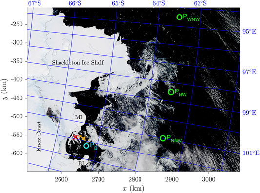
FIGURE 1. Sea ice conditions in the study area and its surroundings on February 10, 2019 (the only day in the analyzed period when the whole region was almost cloudless) in a true-color image from MODIS Terra. The red cross marks the location of the sea ice photograph analyzed in this work (Figure 2). Orange points show locations where ice freeboard data are available. ${\text{P}}_{\text{WNW}}$, ${\text{P}}_{\text{NW}}$ and ${\text{P}}_{\text{NNW}}$ mark grid points of the WaveWatchIII model and ${\text{P}}_{\text{B}}$ is the point at the entrance to the bay used in the wave and weather data analysis. MI = Mill Island, BI = Bowman Island.

The analyzed image is unique not only in terms of its high resolution, but also in terms of the properties of ice floes it contains. In most works devoted to the identification of ice floes in satellite/airborne images the floes span a wide range of sizes, have rounded shapes and the spaces between them are filled with slush/brash ice or very small floes that cannot be identified at the spatial resolution of a given image (e.g., Toyota et al., 2006; Steer et al., 2008; Gherardi and Lagomarsino, 2015; Toyota et al., 2016; Wang et al., 2016). All those features suggest a long deformation history–in granular materials, rounded shapes and a wide size distribution of grains are a signature of grinding under combined shear and compressive stress. The floes analyzed in this study have opposite features: angular, polygonal (often nearly rectangular) shapes, similar sizes and are surrounded by relatively clear water with only a limited number of very small ice pieces between them. Therefore, identification of individual floes in the image is relatively straightforward. We analyze selected geometrical properties of the floes (elongation, rectangularity, etc.) and, following the analysis by Herman et al. (2018), show that the FSD in different regions of the image can be represented by a probability distribution defined as a weighted sum of two components, a Gaussian and a tapered power law. In the discussion section, we use several additional data sources in order to reconstruct the weather, wave and ice conditions in the 2-week period preceding the analyzed date, and we argue that the three different “populations” of floes visible in the image originate from individual wave-induced breakup events. Finally, theoretical arguments and a series of numerical simulations of wave propagation in sea ice, performed with a scattering model based on the Matched Eigenfunction Expansion Method (MEEM; Kohout et al., 2007; Kohout and Meylan, 2008), are used to show that the observed dominating floe sizes in the three different regions of the image (18, 13 and 51 m, respectively) agree with those expected as a result of wave-induced breaking of landfast ice.

The structure of the paper is as follows: Section 2 contains a description of the analyzed satellite image and the method of floe identification (Section 2.1), as well as a list of other, auxiliary data sources (Section 2.2). A detailed description and analysis of selected geometric properties of the ice floes and the floe size distributions in different sectors of the image is provided in Section 3. The discussion in Section 4 groups those parts of the analysis which, due to unavailability or incompleteness of relevant sea ice and/or wave data, are necessarily based on additional assumptions and therefore have a polemical aspect: the ice breakup scenario (Section 4.1) and the results of MEEM simulations (Section 4.2). Finally, concluding remarks can be found in Section 5.

2 Data and Methods

2.1 Sea Ice Floe Data

As mentioned in the introduction, the main source of data for this work is a very high resolution optical satellite image of sea ice floes in the area of study (Figure 2). It was acquired on February 16, 2019 by one of the commercial satellites operated by Maxar Technologies (https://www.maxar.com/), and purchased from Overview (https://www.over-view.com/). The image is centered around 65.55398°S, 101.9066°E (red cross in Figure 1), its spatial resolution equals 0.3 m and image dimensions are 18570 × 5087 pixels, i.e., 5571.0 m × 1526.1 m. A low-resolution version of the image is shown in Figure 2A, more detailed version can be found in Supplementary Figure S1.

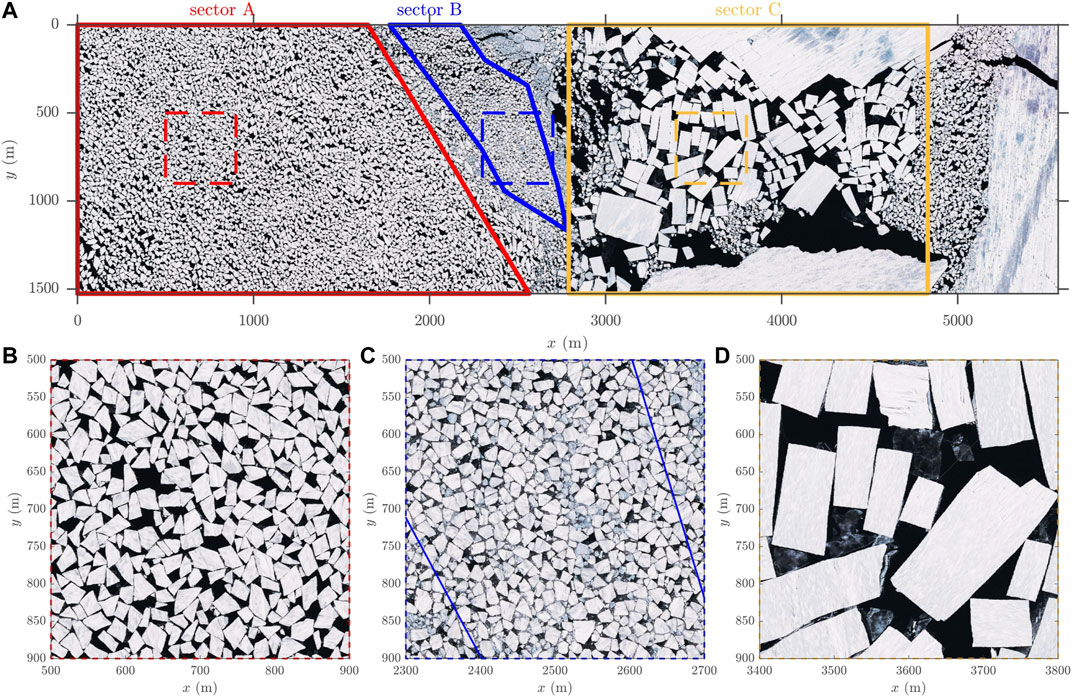
FIGURE 2. The analyzed sea ice photograph from February 16, 2019 (see Figure 1 for location) with borders of the three study regions A, B, and C (continuous lines). The dashed contours in (A) mark the location of zoomed fragments shown in (B–D).

Based on a visual inspection of the image, three sectors have been defined for a detailed analysis, labelled A, B and C (Figure 2A). Sector A contains angular, light-colored ice floes with almost no darker ice or slush in spaces between them. In sector B, the floes are visibly smaller, more densely packed and they have more-rounded shapes. Moreover, some of the floes have darker, blueish color. Sector C is predominantly filled with very large, approximately rectangular floes. Small, irregularly shaped floes can be found only along the leftmost and rightmost boundary of that sector, as well as within a compact patch in its middle-lower part, but not between the very large floes, indicating that the small floes have drifted into that area from the other regions and are not a product of breaking of the large floes. Therefore, only the largest floes from sector C are analyzed further. Overall, the boundaries of the three sectors are defined so that the floes in each of them can be assumed to form a single “population” with statistical properties that are uniform spatially.

Due to the properties of the ice in the image, described above, identification of individual ice floes is relatively trivial. In all three cases, the fragment of the image corresponding to the given sector was transformed to gray-scale and then segmented into three classes–open water, light ice and dark ice–with the k-means clustering method (Table 1). Patches of dark ice surrounded by light ice have been reclassified as parts of ice floes, the remaining ones, together with open water, as “the rest”. A binary image obtained in this way was subjected to several subsequent cycles of automatic object identification in Matlab and manual corrections of floe boundaries in ImageJ. After each cycle, several geometric properties of the identified objects were computed, which helped to detect anomalously shaped and/or large objects, i.e., clusters of touching floes erroneously classified as a single floe. Black pixels representing the “missing” boundaries were then manually inserted in ImageJ.

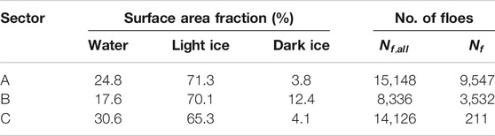
TABLE 1. Summary of ice types and number of objects identified in sectors A–C.

The total number of objects $N_{f,\text{all}}$ identified in each sector is given in Table 1. In the case of sectors A and B, that number includes many very small ice fragments, only a few pixels in size. Before the subsequent analysis, all fragments with width smaller than two pixels (0.6 m) are excluded, resulting in $N_f=\mathrm{9,547}$ and $N_f=\mathrm{3,532}$ floes in sectors A and B, respectively. As already mentioned, only the large floes are taken into account in sector C $\left(N_f=211\right)$, which make only a small fraction of all identified objects, but constitute the large majority of the total ice area in sector C.

2.2 Other Data Sources

In order to aid the interpretation of the floe size data in the analyzed image (Sections 4.1,4.2), additional data sources are used, providing information on weather, sea ice and wave conditions in the surroundings of the area of study.

The weather data, in the form of 1-hourly time series of 2-m air temperature T and 10-m wind speed $V_{10}$ and direction ${\theta }_{10}$ in a point located in the middle of the bay ($P_{\text{B}}$ in Figure 1) are extracted from the results of the Antarctic Mesoscale Prediction System (AMPS; Powers et al., 2012, https://www.earthsystemgrid.org/project/amps.html), a real-time mesoscale modeling system providing numerical forecasts for the Antarctic at 8-km resolution, run at the Mesoscale and Microscale Meteorology (MMM) Division of the National Center for Atmospheric Research (NCAR) and developed in cooperation with Byrd Polar and Climate Research Center at Ohio State University.

The results of the global spectral wave model WaveWatch III operated at the Pacific Islands Ocean Observing System (PacIOOS; https://www.pacioos.hawaii.edu/waves/model-global/) are used as a source of information on wave conditions in the sector of the Southern Ocean surrounding the bay. The data include the significant wave height $H_s$, peak wave period $T_p$ (from which the deep-water peak wavelength $L_p$ is computed) and peak wave direction ${\theta }_p$. Hourly time series from three locations are used (green circles in Figure 1), located to the WNW, NW and NNW from the entrance to the bay ($P_{\text{WNW}}$, $P_{\text{NW}}$ and $P_{\text{NNW}}$, respectively). The latitude of the points, 63° 30′ S, is selected so that the model results are unaffected by the presence of sea ice. Unfortunately, the model resolution (0.5°) and the insufficient treatment of wave–ice interactions make the modelled wave data in direct vicinity of the bay unreliable (several grid points in the area of interest have missing values or zeros as wave parameters). Therefore, data from points $P_{\text{WNW}}$, $P_{\text{NW}}$ and $P_{\text{NNW}}$ are used, providing reliable open-ocean wave conditions.

Sea ice concentration data from AMSR2 in the form of daily 3.125-km resolution maps was obtained from the service of the University of Bremen (https://seaice.uni-bremen.de/sea-ice-concentration-amsr-eamsr2/; Melsheimer and Spreen, 2019). The maps are used to compute the lengths $L_{\text{ice}}$ of the path traveled by the waves from the three WaveWatchIII locations described above ($P_{\text{WNW}}$, $P_{\text{NW}}$, $P_{\text{NNW}}$) to the point $P_{\text{B}}$ through sea ice of concentration A higher than a given prescribed concentration $A_0$. The path lengths $L_{\text{ice}}$, together with an assumed value of the linear wave attenuation coefficient in the ice ${\alpha }_i=3.38\cdot {10}^{-6}{\text{m}}^{-1}$ [corresponding to the 5th percentile of a large dataset of wave attenuation in sea ice analyzed by Stopa et al. (2018)] are used in Section 4.1 to estimate the ratio of the wave amplitude at $P_B$, $a_{\text{in}}$, to the wave amplitude at one of the points outside, $a_{\text{out}}$.

The only available data from which the thickness of the fast ice in the bay can be estimated are ICESat-2 altimeter observations of sea ice freeboard (https://nsidc.org/data/ATL10/versions/3; Kwok et al., 2020) from Januray 20, 2019 (i.e., 4 weeks before the date of interest) at several locations in the outer parts of the bay (orange points in Figure 1). Altogether, 791 single data points are available in the area between 65.2185–65.4665°S and 101.7621–101.9499°E.

Finally, a series of MODIS Aqua and Terra imagery from the period February 3–16, 2019 is used to assess the evolution of sea ice conditions in the area of study in the two weeks preceding the situation of interest. The images have been obtained through the Worldview platform of the NASA’s Earth Observing System Data and Information System (EOSDIS) (https://worldview.earthdata.nasa.gov/).

3 Floe Shapes and Floe Size Distribution

3.1 Geometric Properties of the Ice Floes

In the following analysis, the minimum and maximum caliper diameters, $w_f$ and $l_f$, shortly referred to as floe width and floe length, respectively, are used as the basic measures of floe size. They are defined as the minimum and maximum distance between parallel tangents touching the opposite sides of a floe. Based on $w_f$, $l_f$ and floe surface area $A_f$, several measures of shape can be constructed. Here, we consider floe rectangularity $r_f=A_f/\left(w_f{l}_f\right)$ and elongation $e_f=l_f/w_f$ (see, e.g., Leppäranta, 2005). Additionally, we estimate the number of sides $n_s$ of each floe, reducing it to an $n_s$-sided polygon by means of the iterative Douglas–Peucker algorithm (e.g., Wu and Marquez, 2003). The method is used e.g., in cartographic generalization to reduce the number of points defining a curve in such a way that the maximum distance between the original curve and the simplified curve (the Hausdorff distance) does not exceed a certain prescribed value ${\mathit{ϵ}}_{\text{max}}$. Here, ${\mathit{ϵ}}_{\text{max}}=\mathit{ϵ}{A}_f^{1/2}$ is used, with $\mathit{ϵ}=0.1$ (the results obtained for $0.05<\mathit{ϵ}<0.2$ are statistically very similar to those presented, although, obviously, the exact values of $n_s$ for individual floes might differ). Importantly, the shape analysis is performed for floes with $w_f\ge 4.5\text{m}$ (i.e., 15 pixels), because the shape properties of the smaller floes are extremely sensitive to very small shifts of the floes’ boundaries and cannot be estimated reliably.

The histograms of $e_f$, $r_f$ and $n_s$ for the three sectors A, B, C are shown in Figure 3. As can be expected from a visual inspection of Figure 2, the combinations of the shape characteristics of those three “populations” of floes are markedly different. The floes in sectors A and C have similar elongation, significantly higher than floes from sector B. At the same time, floes from sectors A and B have very similar rectangularity, significantly lower than floes from sector C. Close to 55% of floes from sector C are classified as tetragons and only 10% have $n_s\ge 6$, whereas this number is as high as 45% for floes in sector B, indicating that many of them are approximately ellipsoidal. In sector A, the great majority (88%) of floes have between four and six sides.

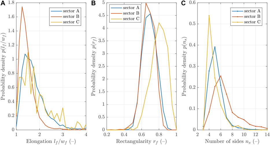
FIGURE 3. Shape characteristics of ice floes from sectors A, B, and C: floe elongation $e_f=l_f/w_f$(A), rectangularity $r_f$(B) and number of sides $n_s$(C).

3.2 Floe Size Distributions

Let l denote any linear measure of floe size ($w_f$, $l_f$, etc.) and $p_l\left(l\right)$ the number-weighted floe size distribution. Following Herman et al. (2018), the general form of $p_l$ considered in this study is a weighted sum of two functions: a tapered power law $p_{PL}\left(l\right)$ and a normal distribution $p_G\left(l\right)$, the relative contribution of each component dependent on the value of $\epsilon \in \left[\mathrm{0,1}\right]$:

The power law component $p_{PL}\left(l\right)$ has the form:

where α denotes the slope and the value of β decides on the onset of the exponential tail at large floe sizes. The Gaussian component $p_G\left(l\right)$ is given by:

where μ and σ denote the mean and standard deviation, respectively. In Eqs 1–3, the coefficients α, β, μ, σ, and ε are adjustable parameters, $\text{Γ}\left(u,x\right)={\displaystyle {\int }_x^{\infty }{t}^{u-1}{e}^{-t}dt}$ is the upper incomplete gamma function, $\text{erf}\left(x\right)=\frac{2}{\sqrt{\pi }}{\displaystyle {\int }_0^x{e}^{-t^2}dt}$ is the error function, and $l_m$ denotes the lowest value of l for which the distributions are valid. The scaling factors in Eqs 2,3 ensure that ${\displaystyle {\int }_{l_m}^{\infty }{p}_{PL}\left(l\right)dl=1}$ and ${\displaystyle {\int }_{l_m}^{\infty }{p}_G\left(l\right)dl=1}$. The corresponding exceedance probabilities $P_{PL}\left(l\right)$ and $P_G\left(l\right)$ are:

and the total exceedance probability $P_l\left(l\right)$ is given by $P_l\left(l\right)=\epsilon P_{PL}\left(l\right)+\left(1-\epsilon \right)P_G\left(l\right)$.

In this work, $w_f$ is used as a representative measure of floe size. In the case of sectors A and B, Eqs 1–3 have been fitted to the data with five adjustable parameters α, β, μ, σ, and ε. In the case of sector C, $\epsilon =0$ is assumed, i.e., only the Gaussian part is considered and $p_l\left(l\right)=p_G\left(l\right)$. The details of the fitting procedure, in which predicted cumulative probabilities are linear-least-squares-fitted to the empirical ones, are described in Herman et al. (2018) and won’t be repeated here. Similarly, the same method as in the previous study–Monte Carlo simulations–is used to obtain the error estimates of the fitted probability distributions.

The results for all three sectors are shown in Figures 4, 5 and in Table 2. Importantly, all fits are very robust, especially in the case of ε, μ and σ, i.e., the relative contribution of the two basic distributions and the properties of the Gaussian part $p_G$. The error estimates of those parameters are at the level of a few percent. In the case of α and β the uncertainties are larger, especially in the case of sector B. This is understandable and can be expected considering that the smallest floes are less reliably identified in the original image, and that the parameters of $p_{PL}$ are very sensitive to the value of the minimal floe size considered. Nevertheless, the obtained values of α (1.48 for sector A, 1.14 for sector B) and β (15.0 and 5.3, respectively) are reasonable and, in the case of α, within the range reported in the literature.

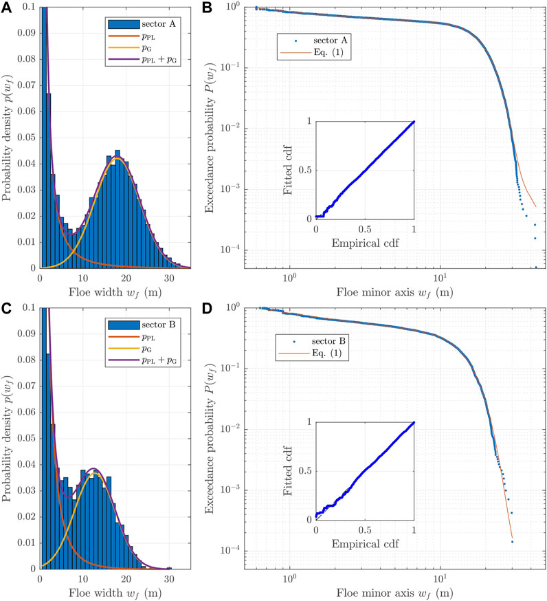
FIGURE 4. Results of the linear least-square fit of predicted and observed cdfs for $w_f$ data from sectors A (A, B) and B (C, D): histograms of $w_f$ with fitted $p_{PL}$, $p_G$ and $p_l$(A, C) and observed exceedance probabilities with fitted $P_l$(B, D). The insets show P–P plots of the fitted vs. observed cdfs. Bin width in (A,C) equals 1 m.

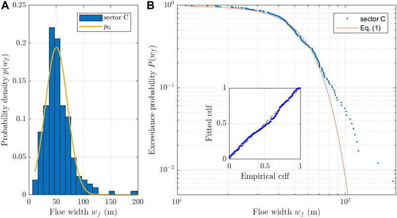
FIGURE 5. As in Figure 4, but for the floe data from sector C. Bin width in (A) equals 10 m.

TABLE 2. Results of least-square fit of Eqs 1–3 to observed FSD data.

Arguably, the size distributions of the larger floes are the particularly interesting aspect of the analyzed dataset. In all three sectors, those distributions are Gaussian, with the mean of ∼18, ∼13 and ∼51 m, respectively. Contrary to most laboratory tests analyzed in Herman et al. (2018), in the present case the Gaussian parts of the total distributions are very well developed and, especially in sector A, clearly separated from the power-law part. In all three sectors, the floes from the size range dominated by the Gaussian part of the FSD contribute over 90% to the total sea ice surface area.

Notably, very similar results are obtained if other size measures are used instead of $w_f$. For example, for $l_f$ in sector A we obtain $\epsilon =0.58$, $\alpha =1.3$, $\beta =4.67$, $\mu =26.82$ and $\sigma =10.51$. Also, if an ellipse is fitted to each floe and the minor and major axes of that ellipse are used instead of $w_f$ and $l_f$, the results remain very similar to those presented above.

4 Discussion

4.1 Weather, Wave and Ice Conditions During the Period of Study

Based on a single image, it is very difficult to draw inferences about the factors that have produced the floes visible in that image. In most situations, the state of the sea ice at any given location and time instance is a product of a long history of thermodynamic and dynamic processes. However, the distinctive shapes and size distributions of the floes from sectors A, B and C of the image analyzed in this study suggest that those floes were formed from continuous, landfast ice by wave-induced breaking, not long before that image was taken. Although several unknowns remain, with the aid of additional data described in Section 2.2 we might attempt to reconstruct those breakup events.

Figure 6 shows a sequence of true-color MODIS images of the bay between the Mill and Bowman islands in the time period preceding February 16, 2019 (more images can be found in the Supplementary Figure S2). During the first week of February, the position of the fast-ice edge in the bay was very stable, and the overall wind and wave conditions in the whole area were rather calm, with wind speeds below 10 m s⁻¹ (Figure 7), open-ocean wave heights of ∼2 m (Figure 8) and more than 200 km of drifting ice protecting the bay from waves from the prevailingly W–NW directions (Figure 9). During the following days, between 7 and 10 February, very large, elongated fragments, some of them 20 or more kilometers long, detached from the fast ice. Those very large “mega-floes” formed in a series of fracture events, each associated with (at times very strong) offshore winds: E and SE on 7–8 February, SW on 9 February, and S on 10 February (Figures 6B,C, Supplementary Figure S2). This suggests tensile failure of the landfast ice, presumably along preexisting cracks and weaknesses, not visible in the satellite imagery. The net drift of the “mega-floes” during that period was in the westerly direction. On 10–11 February, they accumulated in the area west of 102°E, i.e., in the area where the high-resolution image was taken several days later. Notably, although some of those floes broke into smaller, but still kilometer-size parts, they didn’t undergo strong fragmentation until 10 February–their shapes can be easily recognized in subsequent MODIS images. Thus, in spite of the fact that the open ocean significant wave height exceeded 5 m twice during the period 8–10 February (Figure 8) and the extent of the drifting ice pack, especially in the WNW direction, decreased rapidly on 8 February (Figure 9), the wave conditions inside the bay must have remained relatively calm. The reason for that is, first, the dominant wave direction (from the west during the maximum wave heights in the night 9/10 February), and second, the relatively short peak period of those waves during the storm maximum (blue line in Figure 8B), for which the attenuation coefficient likely was much higher than for the low-frequency swell observed on other days (i.e., higher than the very low value assumed in Figure 9B).

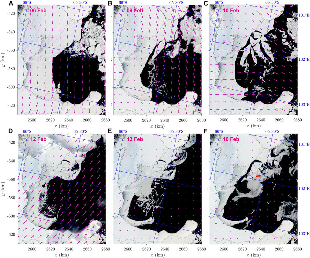
FIGURE 6. Evolution of sea ice conditions in the area of study during the time period preceding February 16, 2019. The red rectangle in (F) marks the boundary of the sea ice image in Figure 2A. The arrows show 10-m AMPS wind vectors at 12:00 UTC on a given day. [Images: (A,C,E): MODIS Terra, (B,D,F): MODIS Aqua.].

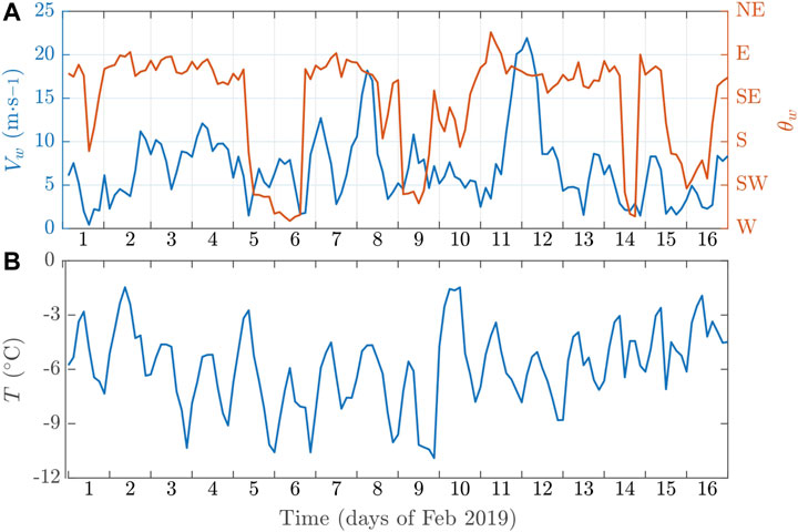
FIGURE 7. Time series of AMPS 10-m wind speed $V_w$ and direction ${\theta }_w$(A) and 2-m air temperature T(B) during the study period (point $P_{\text{B}}$ in Figure 1). The convention for ${\theta }_w$ in (A): ‘W’ = from the west etc.

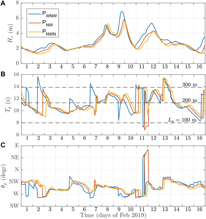
FIGURE 8. Time series of wave conditions during the study period in the three points marked in green in Figure 1: significant wave height $H_s$(A), peak period $T_p$(B) and peak wave direction ${\theta }_p$(C). Dashed lines in (B) mark wave periods corresponding to deep-water wavelengths of 100, 200 and 300 m. The convention for ${\theta }_p$ in (C): ‘W’ = from the west etc.

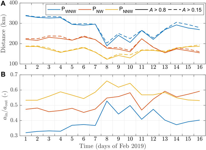
FIGURE 9. Open ocean sea ice conditions during the study period in the region surrounding the bay. (A): the length of the path from points ${\text{P}}_{\text{WNW}}$, ${\text{P}}_{\text{NW}}$, ${\text{P}}_{\text{NNW}}$ (green in Figure 1) to the entrance of the bay (point $P_{\text{B}}$) traveled through sea ice with concentration $A>0.8$ (continuous lines) and $A>0.15$ (dashed lines). (B): the ratio of wave amplitude at the entrance of the bay, $a_{\text{in}}$, to the wave amplitude in points ${\text{P}}_{\text{WNW}}$, ${\text{P}}_{\text{NW}}$, ${\text{P}}_{\text{NNW}}$, $a_{\text{out}}$, estimated from the path lengths in (A) with an attenuation coefficient ${\alpha }_i=3.38\cdot {10}^{-6}{\text{m}}^{-1}$, equal to the 5th percentile of a large dataset of wave attenuation analyzed by Stopa et al. (2018).

The sea ice situation in the bay changed on 11–12 February. In MODIS images from 12 February (Figure 6D) most of the “mega-floes”, especially those neighboring open water, are broken into smaller pieces, so that a high-ice-concentration zone of fragmented ice surrounding the larger floes develops, pushed toward the SW coast of the bay by very strong $\left(>20\text{m}{\text{s}}^{-1}\right)$ ESE wind (Figure 7). Outside of the bay, the wave heights exceeded 4 m in the night 11/12 February and, importantly, their direction varied between WNW and NW (with a very short episode of more northerly directions), as opposed to W–WNW during earlier storms. Evidently, that seemingly small change of direction was sufficient to cause progressive ice breaking in the south-eastern part of the bay. Characteristic narrow stripes of small floes, detaching from the edge of the landfast ice (lower-left part of Figure 6D), drifted with the wind in the westerly direction. One day later, on 13 February, most of the eastern parts of the bay were ice-free, as small floes that had originated in that area moved to the central part of the bay, 30–40 km to the west (Figure 6E). In the subsequent period of weak winds from varying directions, the position and shape of that “cloud” of small floes changed slightly, with the overall westerly drift. On 16 February, the boundary between that cloud and the cluster of large floes remaining from the initial “mega-floes” (still with sizes of kilometers) was located exactly within the area of the image analyzed in this study (red rectangle in Figure 2F).

In summary, the most plausible interpretation of that image is as follows: the floes in sector A originate from the landfast ice in the eastern part of the bay, broken by waves on February 12, 2019; the floes from sector C were broken off the edges of the very large floes (fragments of which are visible in the southern part of the image in Figure 2), probably around the same time as floes in sector A. However, whereas floes from sector A were most probably formed by waves entering the bay from outside (the local fetch in the SE part of the bay on 12 February was close to zero), locally generated waves might have led to breakup of ice in sector C, which at that time was already situated in the western part of the area: with fetch of a few tens of kilometers and wind speeds $U_{10}>20\text{m}{\text{s}}^{-1}$, the expected wave height and peak period are ∼4 m and ∼7 s, respectively, i.e., enough to break the ice of thickness 1–2 m (see next section). The origin of floes from sector B is harder to decipher, but presumably they were formed during the initial stages of the 11/12 February event–that would explain both their location shorewards from floes in sector A and their more rounded shapes indicating longer exposition to wave and wind forcing.

4.2 Observed Floe Sizes as a Result of Wave-Induced Breakup

A very important question related to the scenario proposed above is how the dominant sizes of ice floes in sectors A, B and C (18, 13 and 51 m, respectively) are related to the properties of the sea ice and to the wave forcing that has led to breakup. Unfortunately, there is no available information on sea ice material properties in the study area, and even if the breakup scenario sketched in the previous section is correct, there are no data on the local wave field inside of the bay. In the following, we first estimate the range of realistic values of the relevant variables–sea ice thickness $h_i$ and elastic modulus $E_i$, peak wave period $T_p$ and floe size L relative to the peak wavelength $L_p$—and then compute the size of ice floes resulting from ice breakup for a very large number of combinations of those variables in order to estimate the likelihood of observing the floe sizes seen in the analyzed image. The computation is based on MEEM simulations (Kohout et al., 2007; Kohout and Meylan, 2008), as described below. Alternatively, the coupled wave–ice model by Herman (2017) could be used for that purpose, but it is more expensive computationally, so that, after several tests comparing the two methods, MEEM was selected as an efficient alternative.

As mentioned in Section 2.2, the only available data related to the ice thickness are satellite freeboard measurements from January 20, 2019, from a location at that time covered by landfast ice (orange points in Figure 1). Considering that a uniform ice cover was present in the whole region throughout winter and spring until January, it seems reasonable to assume that the thickness of that ice was spatially uniform, determined primarily by thermodynamic growth, and thus that those measurements are representative for the ice in the whole bay. Moreover, as the temperatures in the analyzed period remained below zero (Figure 7B), it might be assumed that the thickness of the ice remained relatively stable between 20 January and mid-February. The median freeboard from the available data equals $h_f=0.234\text{m}$. Assuming water density ${\rho }_w=1024\text{kg}{\text{m}}^{-3}$ and first-year-ice density ${\rho }_i=915\text{kg}{\text{m}}^{-3}$, an upper limit on ice thickness $h_{i,\text{max}}=2.20\text{m}$ is obtained (for bare ice, i.e., snow thickness $h_s=0$). With snow density ${\rho }_s=300\text{kg}{\text{m}}^{-3}$, $h_i$ varies between 1.53 and 0.87 m for $h_s$ between 0.1 and 0.2 m, and this estimation seems realistic considering typical sea ice thickness and snow depth variability in that region of the Antarctic (Markus et al., 2011). In the case of the elastic modulus $E_i$ of the ice, values between $5\cdot {10}^9$ and $9\cdot {10}^9\text{Pa}$ are considered (Timco and Weeks, 2010).

Altogether, the scattering model was run for all 1,512 possible combinations of the following variables: wave period $T_p=4.0,4.5,5.0,\dots ,14.0\text{s}$, ice thickness $h_i=0.75,1.00,1.25,\dots ,2.00\text{m}$, elastic modulus $E_i=5\cdot {10}^9,7\cdot {10}^9,9\cdot {10}^9\text{Pa}$, relative floe length $L/L_p=\mathrm{3,5,10,50}$ (the smaller values of $L/L_p$ are included in order to take into account the possibility that some of the floes in the image may result from breaking of large, but finite-size floes; the case $L/L_p=50$ represents the landfast ice). A small random value was added to each $L/L_p$ ratio to avoid resonance problems. Regular waves were assumed, a simplification justified by the results of Herman (2017), who showed that irregular waves (Jonswap spectrum) produced essentially identical floe sizes as sine waves with period equal to the peak period of the spectrum. The same incident wave height of 1 m was used in all simulations (see further).

For each combination of parameters, the time series of sea ice vertical excursion $\xi \left(x,t\right)$ was computed (x denotes distance from the ice edge, t denotes time) using modes $-2,-\mathrm{1,0,1},\dots ,100$ obtained with MEEM (using the original mode numbering of Kohout et al., 2007). Based on $\xi \left(x,t\right)$, the maximum bending stress ${\sigma }_{\text{max}}$ was determined as ${\sigma }_{\text{max}}=0.5h_i{E}_i{\text{max}}_{t\in \left[0,T_p\right)}\left|{\partial }^2\xi /\partial x^2\right|$ (see, e.g., Dumont et al., 2011; Voermans et al., 2020). The location of that maximum $x_b$ is treated as the potential breaking position. In the further analysis, only cases with ${\sigma }_{\text{max}}>{\sigma }_{\text{b}}$ were used, with the flexural strength of the ice ${\sigma }_{\text{b}}=0.4\text{MPa}$, typical for first-year ice (e.g., Timco and Weeks, 2010; Voermans et al., 2020). Thus, the obtained dataset (1386 cases, i.e., 92% of the initial 1512) represents situations when incident waves of 1 m height were sufficient to break the ice. As the heights of waves entering the bay from the outside during the relevant time period likely exceeded 1 m (Figure 8A, 9B), and the locally generated waves during the strong wind event on 12 February were higher than 1 m as well, it is reasonable to assume that the dataset includes those situations that actually led to the ice breakup analyzed here. Notably also, varying the incident wave height in MEEM would modify the values ${\sigma }_{\text{max}}$, but not the locations $x_b$ of the maximum bending stress, as the model is linear. Varying the value of ${\sigma }_{\text{b}}$ within the limit typically observed in sea ice (between 0.1 and 0.7 MPa) does not in any way influence the conclusions formulated below.

The histograms of $x_b$ determined for the whole dataset, as well as separately for short- and long-period waves (below and above 8 s, respectively) are shown in Figure 10. Obviously, those histograms cannot be treated as probability distributions, as some of the considered combinations of wave/ice conditions are more probable than others. In spite of that limitation, however, the results do provide useful insight into the expected variability of floe sizes within the analyzed range of conditions. The very close correspondence between the observed dominating floe size in sector A (17.9 m) and the maximum of the $x_b$ histogram (16.3 m) is remarkable. Overall, the values of $x_b$ between 11 and 26 m constitute ∼50% of all cases considered; in ∼90% of cases the obtained floe size is smaller than 60 m. Thus, the floe sizes observed in this case study can be regarded as expected under the conditions considered. However, the very close similarity of the histograms representing short and long waves means that based on the resulting floe size alone it is not possible to determine whether the ice from which those floes were formed was broken by long, open ocean or short, locally generated waves. In both cases the expected floe sizes are very similar. Crucially, they are much lower than half-wavelength in the first case, but comparable with half-wavelength in the second case (the wave periods corresponding to deep-water half-wavelengths equal to the mean floe sizes in sectors A, B and C are 4.8, 4.1 and 8.1 s, respectively).

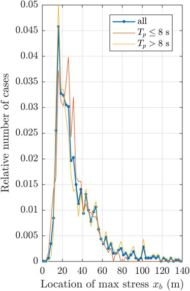
FIGURE 10. Results of MEEM simulations: histogram of the locations $x_b$ of maximum bending stress relative to the ice edge for all wave periods considered, $4\le T_p\le 14\text{s}$ (blue) and separately for short (red; $T_p\le 8$ s) and long (yellow; $T_p>8\text{s}$) waves.

5 Concluding Remarks

The sea ice breakup event that produced floes analyzed in this case study provides a very good example of breaking resulting in narrow, Gaussian distributions of fragment sizes–as opposed to more widely analyzed situations when the fragment size distributions are heavy-tailed, often covering several orders of magnitude. Remarkably, the Gaussian parts of the FSDs analyzed here, based on real-world data, are better developed and represent larger fractions of the total sea ice surface area than was the case in the laboratory study by Herman et al. (2018), where the distribution Eqs 1–3 was first proposed for describing FSDs in sea ice broken by waves. Further studies and more observational evidence are necessary to estimate the range of conditions in which the FSDs of the type considered here are likely to occur. Based on the available data, as well as results of theoretical and numerical studies on granular materials, it seems reasonable to assume that the Gaussian FSD combined with angular floe shapes can be treated as a signature of sea ice freshly broken by waves. Subsequent breaking and diminution of those polygonal floes due to their interactions under compressive and/or shear stress gradually produces the more commonly observed, rounded floe shapes and wide, upper-truncated FSDs with a large fraction of very small fragments. Sector B of the image analyzed here seems to represent an example of sea ice in that transitional phase, with still limited, but noticeable effects of “grinding” after the initial breakup.

As discussed in the previous section, the results of the scattering model suggest that, based on the resulting floe sizes, little can be inferred about the period and length of the waves that had led to breaking–similar floes can be produced by long open-ocean swell and local wind waves. As noted in the introduction, this finding is not surprising in view of the available qualitative evidence, theoretical arguments and modeling results (Squire, 1984; Squire et al., 1995; Langhorne et al., 1998; Montiel and Squire, 2017; Herman, 2017; Herman et al., 2018, and references there). In the case analyzed here, as we argue in Section 4.1, floes from sectors A, B and C, although presumably formed during the same storm event, might have been produced by different wave “systems”, originating outside or inside of the bay. Those difficulties in identifying relationships between the wave forcing and the resulting floe size clearly show the need for more comprehensive observational data, including details of meteorological and wave conditions, as well as sea ice properties.

Data Availability Statement

The datasets presented in this study can be found in online repositories. The names of the repository/repositories and accession number(s) can be found below: https://doi.org/10.34808/h3ye-4d45.

Author Contributions

AH planned the research, processed the sea ice image, analyzed the floe size data and wrote the manuscript. MW prepared the additional sea ice and weather data. SC developed the code of the MEEM model. All authors contributed to manuscript revision, read, and approved the submitted version.

Funding

This work has been financed by Polish National Science Centre project no. 2018/31/B/ST10/00195 (“Observations and modeling of sea ice interactions with the atmospheric and oceanic boundary layers”).

Conflict of Interest

The authors declare that the research was conducted in the absence of any commercial or financial relationships that could be construed as a potential conflict of interest.

Acknowledgments

The analyzed sea ice image was acquired by Maxar Technologies (https://www.maxar.com/) and purchased from Overview (https://www.over-view.com/). The MODIS images are available through the Worldview platform of the NASA’s Earth Observing System Data and Information System (EOSDIS, https://worldview.earthdata.nasa.gov/). The Antarctic Mesoscale Prediction System (AMPS) data can be accessed through the NCAR’s Climate Data Gateway at https://www.earthsystemgrid.org/project/amps.html. WaveWatch III results are available at the Pacific Islands Ocean Observing System (PacIOOS, https://www.pacioos.hawaii.edu/waves/model-global/). The ICESat-2 altimeter observations of sea ice freeboard are available at https://nsidc.org/data/ATL10/versions/3. The sea ice concentration data can be downloaded from PANGAEA at https://doi.org/10.1594/PANGAEA.898400. We thank the Reviewers for their insightful comments on the first version of our manuscript.

Supplementary Material

The Supplementary Material for this article can be found online at: https://www.frontiersin.org/articles/10.3389/feart.2021.655977/full#supplementary-material

References

Alberello, A., Onorato, M., Bennetts, L., Vichi, M., Eayrs, C., MacHutchon, K., et al. (2019). Pancake Ice Floe Size Distribution during the Winter Expansion of the Antarctic Marginal Ice Zone. The Cryosphere 13, 41–48. doi:10.5194/tc-13-41-2019
Ardhuin, F., Otero, M., Merrifield, S., Grouazel, A., and Terrill, E. (2020). Ice Breakup Controls Dissipation of Wind Waves across Southern Ocean Sea Ice. Geophys. Res. Lett. 47, e2020GL087699. doi:10.1029/2020GL087699
Bateson, A., Feltham, D., Schröder, D., Hosekova, L., Ridley, J., and Aksenov, Y. (2020). Impact of Floe Size Distribution on Seasonal Fragmentation and Melt of Arctic Sea Ice. The Cryosphere 14, 403–428. doi:10.5194/tc-14-403-2020
Bennetts, L., Peter, M., Squire, V., and Meylan, M. (2010). A Three-Dimensional Model of Wave Attenuation in the Marginal Ice Zone. J. Geophys. Res. 115, C12043. doi:10.1029/2009JC005982
Bennetts, L., and Squire, V. (2012). Model Sensitivity Analysis of Scattering-Induced Attenuation of Ice-Coupled Waves. Ocean Model. 45–46, 1–13. doi:10.1016/j.ocemod.2012.01.002
Boutin, G., Ardhuin, F., Dumont, D., Sévigny, C., Girard-Ardhuin, F., and Accensi, M. (2018). Floe Size Effect on Wave–Ice Interactions: Possible Effects, Implementation in Wave Model, and Evaluation. J. Geophys. Res. 123, 013622. doi:10.1029/2017JC013622
Boutin, G., Williams, T., Rampal, P., Olason, E., and Lique, C. (2020). “Impact of Wave-Induced Sea Ice Fragmentation on Sea Ice Dynamics in the MIZ,” in Proc. 25th IAHR Int. Symp. on Ice, Trondheim, Norway, 23–25 Nov 2020. Editors K. Alfredsen, K. V. Hoyland, W. Lu, P. L. Bjerke, L. Lia, and S. Loset (IAHR), 11.
Collins, C., Rogers, W., Marchenko, A., and Babanin, A. (2015). In situ measurements of an Energetic Wave Event in the Arctic Marginal Ice Zone. Geophys. Res. Lett. 42, 1863–1870. doi:10.1002/2015GL063063
Dolatshah, A., Nelli, F., Bennetts, L., Alberello, A., Meylan, M., Monty, J., et al. (2018). Hydroelastic Interactions between Water Waves and Floating Freshwater Ice. Phys. Fluids 30, 091702. doi:10.1063/1.5050262
Dumas-Lefebvre, E., and Dumont, D. (2020). Aerial Observations of Sea Ice Breakup by Ship-Induced Waves. ArcticNet Annu. Sci. Meet., 7–10. doi:10.13140/RG.2.2.23493.40164 Dec 2020
Dumont, D., Kohout, A., and Bertino, L. (2011). A Wave-Based Model for the Marginal Ice Zone Including Floe Breaking Parameterization. J. Geophys. Res. 116, C04001. doi:10.1029/2010JC006682
Geise, G., Barton, C., and Tebbens, S. (2016). Power Scaling and Seasonal Changes of Floe Areas in the Arctic East Siberian Sea. Pure Appl. Geophys. 174, 1–10. doi:10.1007/s00024-016-1364-2
Gherardi, M., and Lagomarsino, M. (2015). Characterizing the Size and Shape of Sea Ice Floes. Sci. Rep. 5, 10226. doi:10.1038/srep10226
Herman, A. (2012). Influence of Ice Concentration and Floe-Size Distribution on Cluster Formation in Sea Ice Floes. Cent. Europ. J. Phys. 10, 715–722. doi:10.2478/s11534-012-0071-6
Herman, A. (2011). Molecular-dynamics Simulation of Clustering Processes in Sea-Ice Floes. Phys. Rev. E 84, 056104. doi:10.1103/PhysRevE.84.056104
Herman, A. (2013). Numerical Modeling of Force and Contact Networks in Fragmented Sea Ice. Ann. Glaciology 54, 114–120. doi:10.3189/2013AoG62A055
Herman, A. (2021). Spectral Wave Energy Dissipation Due to Under-ice Turbulence. J. Phys. Oceanogr. 51, 1177–1186. doi:10.1175/JPO-D-20-0171.1
Herman, A. (2017). Wave-induced Stress and Breaking of Sea Ice in a Coupled Hydrodynamic–Discrete-Element Wave–Ice Model. The Cryosphere 11, 2711–2725. doi:10.5194/tc-11-2711-2017
Herman, A., Evers, K.-U., and Reimer, N. (2018). Floe-size Distributions in Laboratory Ice Broken by Waves. The Cryosphere 12, 685–699. doi:10.5194/tc-12-685-2018
Horvat, C., Roach, L., Tilling, R., Bitz, C., Fox-Kemper, B., Guider, C., et al. (2019). Estimating the Sea Ice Floe Size Distribution Using Satellite Altimetry: Theory, Climatology, and Model Comparison. The Cryosphere 13, 2869–2885. doi:10.5194/tc-13-2869-2019
Horvat, C., Tziperman, E., and Campin, J. (2016). Interaction of Sea Ice Floe Size, Ocean Eddies, and Sea Ice Melting. Geophys. Res. Lett. 43, 8083–8090. doi:10.1002/2016GL069742
Horvat, C., and Tziperman, E. (2017). The Evolution of Scaling Laws in the Sea Ice Floe Size Distribution. J. Geophys. Res. 122, 7630–7650. doi:10.1002/2016JC012573
Inoue, J., Wakatsuchi, M., and Fujiyoshi, Y. (2004). Ice Floe Distribution in the Sea of Okhotsk in the Period when Sea-Ice Extent Is Advancing. Geophys. Res. Lett. 31, L20303. doi:10.1029/2004GL020809
Kohout, A., and Meylan, M. (2008). An Elastic Plate Model for Wave Attenuation and Ice Floe Breaking in the Marginal Ice Zone. J. Geophys. Res. 113, C09016. doi:10.1029/2007JC004434
Kohout, A., Meylan, M., Sakai, S., Hanai, K., Leman, P., and Brossard, D. (2007). Linear Water Wave Propagation through Multiple Floating Elastic Plates of Variable Properties. J. Fluids Structures 23, 649–663. doi:10.1016/j.jfluidstructs.2006.10.012
Kohout, A., Williams, M., Toyota, T., Lieser, J., and Hutchings, J. (2016). In situ observations of Wave-Induced Sea Ice Breakup. Deep Sea Res. 131, 22–27. doi:10.1016/j.dsr2.2015.06.010
[Dataset] Kwok, R., Cunningham, G., Markus, T., Hancock, D., Morison, J., Palm, S., et al. (2020). ATLAS/ICESat-2 L3A Sea Ice Freeboard, Version 3. Boulder, Colorado USA: NSIDC: National Snow and Ice Data Center. doi:10.5067/ATLAS/ATL10.003 (Accessed Jan 02, 2021)
Langhorne, P., Squire, V., Fox, C., and Haskell, T. (1998). Break-up of Sea Ice by Ocean Waves. Ann. Glaciology 27, 438–442.
Li, J., Babanin, A., Liu, Q., Voermans, J., Heil, P., and Tang, Y. (2021). Effects of Wave-Induced Sea Ice Break-Up and Mixing in a High-Resolution Coupled Ice-Ocean Model. J. Mar. Sci. Engng. 9, 365. doi:10.3390/jmse9040365
Lu, P., Li, Z., Zhang, Z., and Dong, X. (2008). Aerial Observations of Floe Size Distribution in the Marginal Ice Zone of Summer Prydz Bay. J. Geophys. Res. 113. doi:10.1029/2006JC003965
Markus, T., Massom, R., Worby, A., Lytle, V., Kurtz, N., and Maksym, T. (2011). Freeboard, Snow Depth and Sea-Ice Roughness in East Antarctica from In Situ and Multiple Satellite Data. Ann. Glaciol. 52, 242–248. doi:10.3189/172756411795931570
[Dataset] Melsheimer, C., and Spreen, G. (2019). AMSR2 ASI Sea Ice Concentration Data, Antarctic, Version 5.4 (NetCDF). doi:10.1594/PANGAEA.898400
Montiel, F., Squire, V., and Bennetts, L. (2016). Attenuation and Directional Spreading of Ocean Wave Spectra in the Marginal Ice Zone. J. Fluid Mech. 790, 492–522. doi:10.1017/jfm.2016.21
Montiel, F., and Squire, V. (2017). Modelling Wave-Induced Sea Ice Breakup in the Marginal Ice Zone. Proc. R. Soc. A. 473, 20170258. doi:10.1098/rspa.2017.0258
Perovich, D., and Jones, K. (2014). The Seasonal Evolution of Sea Ice Floe Size Distribution. J. Geophys. Res. 119, 8767–8777. doi:10.1002/2014JC010136
Powers, J., Manning, K., Bromwich, D., Cassano, J., and Cayette, A. (2012). A Decade of Antarctic Science Support through AMPS. Bull. Am. Meteorol. Soc. 93, 1699–1712. doi:10.1175/BAMS-D-11-00186.1
Prinsenberg, S., and Peterson, I. (2011). Observing Regional-Scale Pack-Ice Decay Processes with Helicopter-Borne Sensors and Moored Upward-Looking Sonars. Ann. Glaciology 52, 35–42. doi:10.3189/172756411795931688
Roach, L., Horvat, C., Dean, S., and Bitz, C. (2018). An Emergent Sea Ice Floe Size Distribution in a Global Coupled Ocean–Sea Ice Model. J. Geophys. Res. 123, 4322–4337. doi:10.1029/2017JC013692
Rothrock, D., and Thorndike, A. (1984). Measuring the Sea-Ice Floe Size Distribution. J. Geophys. Res. 89, 6477–6486.
Squire, V. (2018). A Fresh Look at How Ocean Waves and Sea Ice Interact. Phil. Trans. R. Soc. A. 376, 20170342. doi:10.1098/rsta.2017.0342
Squire, V., Dugan, J., Wadhams, P., Rottier, P., and Liu, A. (1995). Of Ocean Waves and Sea Ice. Annu. Rev. Fluid Mech. 27, 115–168.
Squire, V., and Montiel, F. (2016). Evolution of Directional Wave Spectra in the Marginal Ice Zone: a New Model Tested with Legacy Data. J. Phys. Oceanogr. 46, 3121–3137. doi:10.1175/JPO-D-16-0118.1
Squire, V. (2020). Ocean Wave Interactions with Sea Ice: A Reappraisal. Annu. Rev. Fluid Mech. 52, 37–60. doi:10.1146/annurev-fluid-010719-060301
Squire, V. (2007). Of Ocean Waves and Sea-Ice Revisited. Cold Regions Sci. Tech. 49, 110–133. doi:10.1016/j.coldregions.2007.04.007
Steer, A., Worby, A., and Heil, P. (2008). Observed Changes in Sea-Ice Floe Size Distribution during Early Summer in the Western Weddell Sea. Deep-sea Res. 55, 933–942. doi:10.1016/j.dsr2.2007.12.016
Stern, H., Schweiger, A., Stark, M., Zhang, J., Steele, M., and Hwang, B. (2018). Seasonal Evolution of the Sea-Ice Floe Size Distribution in the Beaufort and Chukchi Seas. Elementa 6, 48. doi:10.1525/elementa.305
Stopa, J., Sutherland, P., and Ardhuin, F. (2018). Strong and Highly Variable Push of Ocean Waves on Southern Ocean Sea Ice. Proc. Nat. Acad. Sci. 115, 5861–5865. doi:10.1073/pnas.1802011115
Timco, G., and Weeks, W. (2010). A Review of the Engineering Properties of Sea Ice. Cold Regions Sci. Technol. 60, 107–129. doi:10.1016/j.coldregions.2009.10.003
Toyota, T., Haas, C., and Tamura, T. (2011). Size Distribution and Shape Properties of Relatively Small Sea-Ice Floes in the Antarctic Marginal Ice Zone in Late Winter. Deep Sea Res. 9–10, 1182–1193. doi:10.1016/j.dsr2.2010.10.034
Toyota, T., Kohout, A., and Fraser, A. (2016). Formation Processes of Sea Ice Floe Size Distribution in the Interior Pack and its Relationship to the Marginal Ice Zone off East Antarctica. Deep Sea Res. 131, 28–40. doi:10.1016/j.dsr2.2015.10.003
Toyota, T., Takatsuji, S., and Nakayama, M. (2006). Characteristics of Sea Ice Floe Size Distribution in the Seasonal Ice Zone. Geophys. Res. Lett. 33, L02616. doi:10.1029/2005GL024556
van den Berg, M., Lubbad, R., and Løset, S. (2019). The Effect of Ice Floe Shape on the Load Experienced by Vertical-Sided Structures Interacting with a Broken Ice Field. Mar. Struct. 65, 229–248. doi:10.1016/j.marstruc.2019.01.011
Voermans, J., Rabault, J., Filchuk, K., Ryzhov, I., Heil, P., Marchenko, A., et al. (2020). Experimental Evidence for a Universal Threshold Characterizing Wave-Induced Sea Ice Break-Up. The Cryosphere 14, 4265–4278. doi:10.5194/tc-14-4265-2020
Wang, Y., Holt, B., Rogers, W., Thomson, J., and Shen, H. (2016). Wind and Wave Influences on Sea Ice Floe Size and Leads in the Beaufort and Chukchi Seas during the Summer-Fall Transition 2014. J. Geophys. Res. 121. doi:10.1002/2015JC011349
Wenta, M., and Herman, A. (2019). Area-averaged Surface Moisture Flux over Fragmented Sea Ice: Floe Size Distribution Effects and the Associated Convection Structure within the Atmospheric Boundary Layer. Atmosphere 10, 654. doi:10.3390/atmos10110654
Wenta, M., and Herman, A. (2018). The Influence of Spatial Distribution of Leads and Ice Floes on the Atmospheric Boundary Layer over Fragmented Sea Ice. Ann. Glaciol. 59, 213–230. doi:10.1017/aog.2018.15
Williams, T., Bennetts, L., Squire, V., Dumont, D., and Bertino, L. (2013). Wave-ice Interactions in the Marginal Ice Zone. Part 1: Theoretical Foundations. Ocean Model. 71, 81–91. doi:10.1016/j.ocemod.2013.05.010
Williams, T., Rampal, P., and Bouillon, S. (2017). Wave–ice Interactions in the neXtSIM Sea-Ice Model. The Cryosphere 11, 2117–2135. doi:10.5194/tc-11-2117-2017
Keywords: sea ice, floe size distribution, sea ice breaking, sea ice-waves interactions, satellite imagery, East Antarctic coast
Citation: Herman A, Wenta M and Cheng S (2021) Sizes and Shapes of Sea Ice Floes Broken by Waves–A Case Study From the East Antarctic Coast. Front. Earth Sci. 9:655977. doi: 10.3389/feart.2021.655977
Received: 19 January 2021; Accepted: 04 May 2021;
Published: 17 May 2021.
Edited by:
Giulia Castellani, Alfred Wegener Institute Helmholtz Centre for Polar and Marine Research (AWI), GermanyReviewed by:
Luke Bennetts, University of Adelaide, AustraliaDany Dumont, Université du Québec à Rimouski, Canada
Copyright © 2021 Herman, Wenta and Cheng. This is an open-access article distributed under the terms of the Creative Commons Attribution License (CC BY). The use, distribution or reproduction in other forums is permitted, provided the original author(s) and the copyright owner(s) are credited and that the original publication in this journal is cited, in accordance with accepted academic practice. No use, distribution or reproduction is permitted which does not comply with these terms.
*Correspondence: Agnieszka Herman, agnieszka.herman@ug.edu.pl