
Structural Panel Bayesian VAR with Multivariate Time-Varying Volatility to Jointly Deal with Structural Changes, Policy Regime Shifts, and Endogeneity Issues


Department of Political Science, LUISS Guido Carli University, CEFOP-LUISS, 00197 Rome, Italy
Econometrics 2021, 9(2), 20; https://doi.org/10.3390/econometrics9020020
Submission received: 30 November 2020
/
Revised: 23 March 2021
/
Accepted: 27 April 2021
/
Published: 2 May 2021
(This article belongs to the Special Issue Topics in Computational Econometrics and Finance: Theory and Applications)
Abstract
:This paper improves a standard Structural Panel Bayesian Vector Autoregression model in order to jointly deal with issues of endogeneity, because of omitted factors and unobserved heterogeneity, and volatility, because of policy regime shifts and structural changes. Bayesian methods are used to select the best model solution for examining if international spillovers come from multivariate volatility, time variation, or contemporaneous relationship. An empirical application among Central-Eastern and Western Europe economies is conducted to describe the performance of the methodology, with particular emphasis on the Great Recession and post-crisis periods. A simulated example is also addressed to highlight the performance of the estimating procedure. Findings from evidence-based forecasting are also addressed to evaluate the impact of an ongoing pandemic crisis on the global economy.
Keywords:
structural panel VAR; Bayesian methods; multivariate time-varying volatility; change-points; endogeneity issues; Central-Eastern and Western EuropeJEL Classification:
A1; C01; E02; H3; N01; O41. Introduction
Vector Autoregressions (VARs) are widely used when studying macroeconomic–financial linkages to detect interdependencies and co-movements among multiple economic time-series. In the simplest form, error terms in the VAR models are assumed to have constant variances. While convenient, assuming time-invariant coefficients and variances, it turns out to be highly restrictive in capturing the evolution and thus the dynamics of multiple economic time-series. When time-varying series are introduced in a VAR to highlight the evolving relationship between multiple economic–financial variables, its state space structure need to be modeled and then used in the empirical analysis to estimate unobserved time variations and volatility. Since allowing time-varying coefficients and/or volatility introduces too many parameters than data points, the literature have proposed random processes to time variations or volatility to deal with the curse of dimensionality (see, for instance, Koop and Korobilis (2016)). The randomness in these time-varying parameters fits sufficiently well with Bayesian methods because the probability that a random sequence of events occurs can be interpreted through a reasonable expectation—representing a state of knowledge—or a quantification of a personal belief. More precisely, in Bayesian statistics, one assumes to know something about the possible values of the parameters of interest prior to seeing the data. Thus, the inputs required for estimating that quantity are prior knowledge (or belief) plus data; contrary to frequentist statistics, where these inputs are represented by the data only.
In this context, multicountry Bayesian VAR (BVAR) models have given a new impulse to the literature to evaluate macroeconomic–financial linkages, to test specification hypotheses (see, for instance, Korobilis (2016)), and to conduct policy exercises (see, e.g., Ciccarelli et al. (2018); Canova and Ciccarelli (2009); Canova et al. (2007, 2012); and Koop (1996)). Nevertheless, although estimation of time-varying structures is feasible with a large homogeneous cross-section, heterogeneous dynamics due to an unexpected shock combined with not directly observed or measured factors make it difficult to exploit cross-sectional information estimating time-series variations in multicountry setups (see, for instance, Koop and Korobilis (2016)). More precisely, these empirical models tend to be non-structural and constrained because of time-invariant or exogenous factors in the system. Thus, when formulating policies or forecasting, it is not possible to identify—for example—the reasons underlying different cross-country reactions given an unexpected shock, the causality between real and financial variables, how additional transmission channels allow shocks to spill over, and how economic and institutional implications matter in driving shock transmission. Furthermore, many economic–financial issues show consistent and dramatic structural breaks associated with events such as economic recessions, currency crises, and epidemiology (such as the current COVID-19 pandemic). Such changes in regime are—even now—the core to some of the most important questions in macroeconomics. Recent empirical studies on the conduct of monetary policy along with fiscal consolidation periods have pointed out significant policy paradigm shifts and their implications over the past decades (see, e.g., Cette et al. (2016); Foerster and Matthes (2020); Stock and Watson (2012); Coibion and Gorodnichenko (2012); and Daly et al. (2016)). These shifts seem to have concerned strategy and policy development, monetary policy shocks, and policy interactions. Parallel to these shifts, both the volatility linkages between economic–financial data and the uncertainty in financial markets have changed substantially over time as well. For instance, the Great Recession prompted a renewed debate concerning objectives and conduct of policy issues due to structural changes that have taken place. In particular, slower growth led to questions about how the systematic conduct of policy tools should respond to these shifts. An another issue for changing fundamental policy instruments due to structural changes is also related to the economy that tends to shift between periods of high and low growth. These repeated regime changes may not occur very frequently, but needs to be dealt with when performing forecasting and policy-making. More precisely, dynamic models should account for the possibility of future shifts in the growth rate when setting policy. Indeed, if inter-linkages between real and financial sectors are changing how they react as the economy undergoes structural shifts, cross-country interdependencies and feedback effects matter and then need to be accounted for.
Recently, Pacifico (2019b) developed a structural version of the BVAR—labeled as Structural Panel Bayesian VAR (SPBVAR)—in order to deal with model misspecification and unobserved heterogeneity problems when jointly modeling and quantifying multicountry data using the information contained in a large set of endogenous and economic–financial variables1. The SPBVAR model focuses on a state-space factorization structure, where the factors driving the coefficients of the multicountry VAR are restricted to evolve over time as random walks so as to: reduce the number of parameters; allow for the evaluation of permanent shifts; investigate any type of coefficient factors via their interactions; and replace volatility changes by coefficient changes. This latter turns out to be highly restrictive to evaluate multiple time-varying change-points (or structural breaks) when studying macroeconomic and financial time-series. For example, international business cycle dynamics, policy interactions, and interdependencies and co-movements among different sectors and countries have changed substantially during the recent global crisis and successive consolidation periods. In addition, the increasing volatility and uncertainty in financial markets have confirmed the close volatility linkage between economic–financial data and thus the need to investigate shifts in either coefficients or volatility when describing these changes in a time-varying multicountry framework (see, e.g., Primiceri (2005); Canova and Gambetti (2009); Clark (2009); Cogley et al. (2010); and Sims and Zha (2006)).
My approach and empirical application aim to contribute to this debate. More precisely, this paper develops a modified version of the SPBVAR model allowing for multivariate time-varying volatility to deal with three issues jointly: structural changes, policy regime shifts, and endogeneity issues. Specifically, this model takes the name of multicountry SPBVAR with Multivariate Time-varying Volatility (SPBVAR-MTV) and includes two additional components: a set of lagged endogenous variables to investigate fiscal and monetary policy implications and interactions, and—particularly—time-varying log-volatilities to deal with multiple structural breaks and policy regime shifts over time. Concerning the latter, I imply Autoregressive Conditional Heteroskedasticity in Mean (ARCH-M) model effects in the representation of the outcomes, and it would be an useful way of modeling time-varying conditional second moments providing an alternative to the stochastic volatility specification (see, e.g., Cogley and Sargent (2005); Carriero et al. (2019); and Clark (2011)). In contrast to SPBVAR, in the state-space factorization structure, the variance in error terms is allowed to be time-variant and volatility changes are not more replaced by coefficient changes. More precisely, let the framework be multidimensional (panel data analysis), I model the covariance matrix in time-varying log-volatilities interpreting it as having been broken into a collection of smaller matrices (blocks). Every collection is then estimated using a hierarchical (conjugate) prior specification strategy to allow cross-unit interdependent relationships. The computational costs involved in using that specification are moderate since the high dimensionality is avoided via Bayesian inference and Monte Carlo Markov Chain (MCMC) implementations. For instance, Kalman-Filter technique is used to get appropriate posterior distributions for time-varying coefficients and Metropolis–Hastings algorithm is used to draw posteriors for log-volatilities evolving over time. A Structural Normal Linear Regression (SNLR) model is obtained via Bayesian methods to work with smaller systems in which all the regressors are endogenous, observable, directly measured, and time-varying linear combinations of the right-hand variables of the SPBVAR-MTV model. I also account for three more indices2 in order to quantify international spillover effects and thus evaluate their size (or intensity in terms of volatility) and dynamics (or spreading) among countries and sectors over time. The Bilateral Net Spillover Effect (BNSE) is used to account for cross-unit interdependencies, feedback effects from the impulse variables, and temporary or persistent long-run effects of a potential shock (or excess spillover effects). The Systemic Contribution (SC) index is used to evaluate sequential features associated with systemic events. The Total Contagion Index (TCI) is addressed to investigate contagion measures in real economy and financial markets when dealing with both issues of endogeneity (because of omitted variables and unobserved heterogeneity) and volatility (because of policy regime shifts and structural changes).
In this paper, the SPBVAR-MTV model incorporates the econometric literature on standard Time-Varying Parameter Vector Autoregressions (TVP-VARs) with stochastic volatility, become a benchmark model for analysing and forecasting the evolving inter-relationships between multiple macroeconomic variables (see, e.g., Koop et al. (2009); Koop (1996); Liu and Morley (2014); D’Agostino et al. (2013); and Clark and Ravazzolo (2015a)). Despite the empirical success of these flexible time-varying models, they show a relevant limit about their potential and feasible over-parametrization. More precisely, on the methodological side, the literature makes out two popular Bayesian methods for TVP-VARs with stochastic volatility: Marginal Likelihood (ML), evaluating how likely the observed data are occurred within the system, and Deviance Information Criterion (DIC), trading off between model fit and model complexity. As regards ML estimates, they are usually obtained by using the harmonic mean3 of a conditional likelihood4 that tends to have a substantial bias selecting the wrong model (see, for instance, Chan and Grant (2015) and Frühwirth-Schnatter and Wagner (2008)). Concerning DIC procedure, the MCMC integration based on the conditional likelihood tends to associate higher probability to the most complex models (overfitting5).
The methodology proposed in this paper overtakes these limits by using analytical integrations for integrating out the time-varying volatilities. More precisely, integrated likelihood evaluation is achieved by integrating out the time-varying parameters analytically (e.g., Kalman-Filter technique), whereas the log-volatilities are integrated out numerically via importance sampling. The latter consists of two steps: the Metropolis–Hastings algorithm is used to draw posteriors for time-varying log-volatilities from the proposal density distribution, and then the Newton–Raphson (N-R) method6 algorithm is involved to find the maximum of the (log) conditional density. In this way, the computational costs are further reduced focusing on band and sparse matrix algorithms instead of the conventional Kalman filter.
An empirical application is developed by accounting for the Central, Eastern, and Western European (CEWE) countries in order to include a large pool of advanced and emerging economies, with particular emphasis to the Great Recession and successive post-crisis periods. The United States (US) are included in the analysis to assess international spillover effects and possible contagion measures among financial markets. In this study, I focus on the latest two alternative monetary policy regimes that have been in place since the 1990 (see, for instance, Kallianiotis (2019)): the Inflation Stabilization Era (ISE) from 1994 to 2008 and the Zero Interest Rate Era (ZIRE) from 2008 to 2015. I also consider two more additional periods: 2006q1–2009q4 to investigate possible commonality between financial markets and real economy during the Great Recession and 2010q1–2018q4 to evaluate fiscal implications and policy perspectives during post-crisis consolidation. Moreover, since most of countries joined in with Euro Area (EA), one is also able to investigate how policy regime shifts and endogeneity issues matter when studying macroeconomic–financial linkages. The analysis focuses on five main questions. First, I investigate how different economic–institutional characteristics affect the transmission of fiscal and monetary policy shocks among countries and sectors. Second, I investigate how policy interactions affect the benefits of consolidation among countries. Third, I evaluate how endogeneity and volatility issues affect inter-sector and inter-country linkages in panel setups. Fourth, I evaluate the role of policy regime shifts and their interactions when structural changes and contagion effects matter.
A simulated experiment—compared to related works—is also addressed to highlight the performance of the estimating procedure developed in this study using some Monte Carlo simulations. The findings prove that the hierarchical structural framework with time-varying log-volatilities perform better conditional forecasts when studying macroeconomic–financial linkages with structural breaks and volatility changes.
The remainder of this paper is organized as follows. Section 2 introduces the econometric model, its features, and the estimation procedure. Section 3 describes the dynamic analysis focusing on prior assumptions strategy, posterior distributions, and MCMC implementations. Section 4 presents the data and the empirical analysis. Section 5 addresses a counterfactual assessment on macroeconomic–financial linkages in multicountry dynamic setups by investigating in depth how structural changes and policy regime shifts affect the spreading and the evolution of international spillover effects, with particular attention on triggering events and policy recommendations for decision makers. Section 6 provides a simulated example through Monte Carlo simulations to demonstrate the performance of the estimation method compared to some related existing approaches. The final section contains some concluding remarks.
2. Econometric Model
Compared to Pacifico (2019b), I extend and improve the standard version of the multicountry SPBVAR model in order to jointly account for time-varying parameters and multivariate volatility evolving over time.
Thus, the SPBVAR-MTV model developed in this study includes two additional components: a set of lagged endogenous variables in order to assess different policy regimes and their interactions and time-varying log-volatilities to capture further evolving inter-relationships between multiple economic–financial data. The model has the form:
where the subscripts are country indices, denotes time, L stands for the lag operator, is an vector of intercepts for each i, the subscripts () denote the endogenous variables in each equation within the system observed for i, with () referring to the ones observed for j and independent of i, and is an vector of disturbance terms.
Given the SPBVAR-MTV in (1), all variables within the system are so defined. (i) is an vector of outcomes to be predicted for each i for a given m. (ii) is an matrix of coefficients for each pair of countries for a given m, with , and is an vector of observed lagged variables for each i for a given m to address economic–financial issues. More precisely, stacking for m, I decompose it in , with denoting lagged outcomes to capture the persistence and including lagged control variables such as general economic–financial conditions. (iii) is an matrix of coefficients for each pair of countries for a given q, with , and is an vector including a set of (directly) observed lagged variables for each i for a given q to evaluate economic–institutional interdependencies (such as additional transmission channels). (iv) is an matrix of coefficients for each pair of countries for a given , with , and is an vector including a set of additional (directly) observed lagged variables for each i for a given to evaluate policy implications and interactions (such as policy tools). (v) is an matrix of coefficients for each pair of countries for a given , with , and is an vector including a set of observed lagged proxy7 variables for each i for a given to address further economic–financial linkages (e.g., territorial competitiveness and infrastructural system) and economic–institutional implications (e.g., competitiveness developments and macroeconomic imbalances). Here, all variables in the system are endogenous and time-varying.
The two main differences with respect to a standard SPBVAR lie in the additional component and – particularly – in the variance-covariance matrix of the vector of innovations (). More precisely, , where denotes the time-varying log-volatilities stacked for i and following a random walk process:
where is a block diagonal covariance matrix and denotes the initial conditions to be estimated. More precisely, the matrix is broken into a collection of smaller matrices (blocks). Such a specification implies Autoregressive Conditional Heteroskedasticity in Mean (ARCH-M) model effects in the representation of , and it would be an useful way of modeling time-varying conditional second moments providing an alternative to the stochastic volatility specification. The main novelty in this study is that, in the state-transition Equation (2), the variance in and then volatility changes are allowed to be time-variant. The random-walk assumption in (2) is very common in the time-varying VAR literature, having the advantage of focusing on permanent shifts and reducing the number of parameters in the estimation procedure. In addition, the block diagonality of guarantees the identifiability of the log-volatilities (). The computational costs involved in using that specification are then moderate using hierarchical (conjugate) priors through Bayesian inference and obtain posterior distributions via MCMC algorithms.
In Equation (1), the dynamic relationships are allowed to be unit-specific and all the (potential) structural changes are allowed to vary over time. In addition, whenever the matrices , , , and differ8 for some L, cross-unit lagged interdependencies and structural time variations matter, and then dynamic feedback and interactions among countries and variables are possible. Thus, the framework of the model (1) makes it able to connect the empirical results to the existing literature and contemporaneous developments when quantifying international business cycles, evaluating policy interactions, and performing conditional forecasting. Nevertheless, even if these features add flexibility to the specification, it is very costly making the number of coefficients of (1) very large. Indeed, they are increased by factors.
Let be the number of all matrix coefficients in each equation of the SPBVAR-MTV model for each pair of countries , a vector can be defined containing all lagged (endogenous) variables in the system for each i. Then, I define an vector containing all columns, stacked into a vector9, of the matrices , , , and for each pair of countries for a given k, with , and denoting the time-varying coefficient vectors, stacked for i, for each country–variable pair. With these specifications, I can express the model (1) in a simultaneous-equation form:
where and are vector containing the observable variables of interest and the random disturbances of the model for each i for a given m, respectively, and contains all lagged time-varying variables within the system stacked in .
Now, because the coefficient vectors in vary in different time periods for each country–variable pair and there are more coefficients than data, it is impossible to eliminate . Thus, to avoid the curse of dimensionality, I adapt the framework in Pacifico (2019b) using a hierarchical factor structure to effectively transform the overparametrized multicountry Structural VAR in (1) into a parsimonious SNLR model. More precisely, I take a flexible Bayesian viewpoint to weakly restrict the coefficients to depend on a low-dimensional vector of observable and time-varying factors (the loadings), which correspond to linear combinations of the right-hand variables of (1), where the forecast errors feature a time-variant heteroskedastic structure. These factors would capture—for example—coefficient variations that are specific to a variable (variable-specific effects), specific to a country given a set of observable and directly measured variables (country-specific effects), common among countries and sectors (common effects), and specific to additional time-varying effects among countries and sectors directly affecting the outcomes in (misspecified effects due to endogeneity issues). Such a reparametrization has three appealing features. First, it reduces the problem of estimating high dimensional (potential) combinations of time-varying coefficients into the problem of estimating a smaller number of loadings on some linear combinations of the right-hand variables of (1). Second, since the loadings of the SNLR model are observable and time-varying linear combinations of the right-hand variables of (1), an estimable hierarchical structure is feasible and suitable for policy purposes and strategies. Third, representing the main thrust of this study, the parsimonious SNRL is able to identify additional common or heterogeneous effects between different countries and sectors that vary over time and directly affect the variables of interest in .
In this study, I assume to have the following factor structure:
where and by construction, are matrices obtained by multiplying the matrix coefficients (), stacked in the vector , by conformable matrices with elements equal to zero and one, with being a numerical index that depends on the typology of the factorization, is an vector of unmodeled variations present in , and , with denoting the covariance matrix of the vector that includes time-varying log-volatilities and as in Kadiyala and Karlsson (1997). In this framework, unobserved heterogeneity and functional forms of misspecification are absorbed in the time-varying coefficient vectors . They are observable smooth linear functions of the lagged variables and thus can be easily estimated with a gain in efficiency and accuracy.
The idea is to shrink to a much smaller dimensional vector , with , containing all the regression coefficients stacked into a vector. In this way, further investigations (e.g., policy regime shifts and interactions, international business cycles, and economic–institutional linkages) can be performed. Finally, the factorization of becomes exact as long as converges to zero.
In Equation (4), all factors are permitted to be time-varying, and thus time-variant structures can be obtained via implementations of MCMC algorithms. Moreover, time variations in the variance of shocks to the factors are also allowed so that can capture (potential) structural changes and policy shifts among countries and variables. Running Equations (3) and (4) for Equation (1), the factorization is:
Given the factorization in Equation (5), the reduced-form SPBVAR-MTV model in Equation (3) can be transformed into a Structural Normal Linear Regression10 model with an error covariance matrix of an Inverse-Wishart () distribution11. By Equations (3) and (4), the SNLR model can be written as
where is an matrix that stacks all coefficients and their possible interactions in the SPBVAR-MTV model in (1), with , and has a particular heteroskedastic covariance matrix that needs to accounted for, with .
To complete the specification, I suppose the following state-space structure for the time-varying regression coefficients:
where , is a block diagonal matrix, and , where controls the tightness (stringent conditions) of the factorization (f) of the time-varying coefficient parameters () in order to make them estimable. Moreover, the computational costs involved in using this specification are moderate since the dimension of is considerably smaller than the dimensionality of , and the block diagonality of guarantees the identifiability of the factors (). Here, some considerations on the innovations are in order: the errors , , and are mutually independent; the error terms and are allowed to be correlated between them; and and are correlated between them by construction.
Finally, if the factorization in Equation (5) is exact, and one has to act on three competing models:
- Model I (): A benchmark model with no change-points, denoting the ‘General Case’.Here, and depends on the only disturbances contained in , with . The would corresponds to the standard SPBVAR, with , , and .
- Model II (): A benchmark model with change-points in the only log-volatilities, denoting the ’Special Case’.Here, and depends on the only disturbances contained in , with . The refers to the case of structural breaks because of (potential) unmodeled dynamics12 in , with , evolving over time, , and uncorrelatedness between the innovations and .
- Model III (): A benchmark model with change-points in either time-varying parameters or log-volatilities, denoting the ’Full Case’.Here, and depends on the disturbances contained in and , with . The refers to the case of structural breaks because of both unmodeled dynamics and policy regime shifts, with , , and evolving over time.
Finally, once the (conditional) marginal likelihood13 is obtained for any model, the exact and final solution can be obtained via MCMC integrations, corresponding to the 14 model solution with higher log Bayes factor (lBF):
where denotes all possible model solutions accounting for the ’General Case’ () with no change-points and refers to all possible model solutions according to the ’Special Case’ () or the ’Full Case’ (). The higher lBF denotes the final solution having higher Posterior Model Probabilities (PMPs)15 according to a generalized version of the Kass and Raftery (1995)’s scale of evidence:
The methodology does not include studies focused on Markov-switching dynamics, modeling covariance matrices of country-specific Markov chains16, because of this paper aims to extend and improve recent works developed when studying macroeconomic–financial linkages in multicountry dynamic panel setups. Nevertheless, to solve potential overfitting problems and cross-unit unobserved heterogeneity, Markov-switching models follow similar hierarchical prior specification strategy proposed in those works, where their empirical results met with positive feedback in the empirical analysis.
2.1. Model Features
To illustrate the conformation of the time-varying SPBVAR-MTV in (1), the exact form and meaning of the ’s and ’s in (4), and the selection of the conformable matrices , I suppose there are endogenous variables and additional observable and proxy variables varying over time for every countries. For convenience, I suppose one lag and no intercept. Thus, the SPBVAR-MTV in (1) assumes the form:
Let be the vector containing all columns (stacked) of the matrices , , , and for each pair of countries , with denoting the variables in each equation observed for j and independent of i, and let be the vector containing all lagged variables in the system for each i for a given k, with .
Concerning the more recent studies of international business cycles and spillover effects (see, e.g., Ciccarelliet al. (2018); Canovaet al. (2012), Pacifico (2019a, 2020a), it is typical for authors to define a country-specific indicator for for each i, a variable-specific indicator for for each m, and a common indicator for for each pair of countries and variables .
According to the empirical implementation addressed in this study, I assess three additional terms in the factorization assuming time-varying log-volatilities in : an indicator to account for the role of additional transmission channels (e.g., in ) affecting spillover effects, the impact of macroeconomic-institutional interdependencies (e.g., in ) in driving the transmission of country-specific shocks, and policy interactions (e.g., in ) when dealing with policy regime shifts; an indicator to investigate heterogeneity, interdependence and commonality among all lagged variables affecting shock transmission; and an indicator to highlight different reactions and co-movements among countries and sectors (, , , ) due to an unexpected common shock.
The factorization is:
where is a vector capturing unaccounted features, is a vector containing all matrix coefficients, stacked in the vector , for each pair of countries for a given k, and, stacking for t, is a vector containing all time-varying coefficient vectors to be estimated. To be more precise: the factors , , and are mutually orthogonal vectors capturing movements in that are country-specific; the factor is an mutually orthogonal vector capturing movements in that are variable-specific, where denotes the number of variable groups; the factor is an mutually orthogonal vector capturing movements in that are common among countries and variables, where denotes the number of common groups. Letting , , , , , and , the conformable matrices in equation (11) can be constructed in this way:
Thus, following some arrangements, the SNLR model is:
Therefore, I obtain five matrices containing all coefficients (stacked) and their possible interactions.
is an observable country-specific indicator for that captures the information contained in the lags of variable M for country 1 and country 2 , with and .
is an observable country-specific indicator for that captures the information contained in a set of lagged variables for country 1 and country 2 , with and , with denoting all possible interactions between the lags of variables M, Q, and .
is an observable country-specific indicator for that captures the information contained in a set of lagged variables for country 1 and country 2 , with and , with denoting all possible interactions between the lags of variables M, Q, , and .
is an observable cross-country variable-specific indicator for that captures, stacked for six groups (), the information contained in the lags of variable and variable . Here: and capture movements between the lags of the only variables M that are specific for variable and variable , respectively; and capture movements between the lags of all variables M, Q, and that are specific for variable and variable , respectively; and and capture movements between the lags of all variables M, Q, , and that are specific for variable and variable , respectively.
is an observable common indicator for that captures, stacked for three groups (), the information contained among countries and variable M (), among countries and variables M, Q, and (), and among countries and variables M, Q, , and (), with , , and .
3. Dynamic Analysis
Before specifying prior assumptions and posterior distributions, I recall the state-space structure of the reparametrized SPBVAR-MTV model in (6):
3.1. Hierarchical Prior Setups and Assumptions
Supposing exact factorization in (5), in order to complete the model, I need to define prior moments on . Thus, collecting them in a vector , with being prior densities, the conditional likelihood function can be derived from the sampling density by using a mixture hierarchical distribution. In other words, a Normal distribution for factors and log-volatilities h; a Wishart distribution for ; and an Inverse-Gamma distribution for and , where . That is,
with depending on the benchmark model: in Model I; in Model II; and in Model III.
Here, , , , and are hyperparamenters, is the sum of the squared errors, with referring to the OLS estimate of , and denotes the least squares estimate of based on the (satured) model, with . Finally, the Equation (18) corresponds to the proposal distribution obtained by MCMC integration (such as Metropolis–Hastings algorithm17).
Since the above-mentioned hierarchical prior specification strategy is affected by common or subjective beliefs because of the marginal effect of economic–financial variables, I assume Independent Normal-Wishart Prior so as to allow cross-equation independence of the coefficients distributions and remove the dependence of on .
Given the state-space structure in Equations (14) and (15), MCMC methods and implementations (such as Gibbs sampling, Kalman Filter algorithm, and Metropolis–Hastings algorithm) can be computed numerically and joint distributions characterised analytically. The first step is to suppose that data run from to in order to obtain a training sample and then to estimate the features of the priors. When such a sample is unavailable, it is just sufficient to modify the expressions for the prior moments in Equations (16)–(20) as:
where
Here, N() stands for a Normal distribution, iW() denotes an Inverse-Wishart distribution, IG() indicates an Inverse-Gamma distribution, and refers to the information available at time . The prior for in (26) and the law of motion for the factors imply that:
where and denote mean and variance-covariance matrix of the conditional distribution of , respectively.
All hyperparameters are known. More precisely, collecting them in a vector , where , they are treated as fixed and are either obtained from the data to tune the prior to the specific applications (such as , , , and ) or selected a priori to produce relatively loose priors (such as , , , , and ). In this context, the only fully Bayesian approach that leads to analytical results requires the use of a natural conjugate prior. According to Equations (16), (17), and (19), the natural conjugate prior has the form18:
where and are hyperparameters collected in the vector , and and are parameters to be estimated.
If , allowing for time-variant factors and volatilities, draws of and can be taken from Normal-Inverse-Gamma distributions.
According to the natural conjugate prior (28), depends on and . Thus, , , and are not independent of one another. To allow different equations in the VAR to have different explanatory variables, previous specifications have to be modified. More precisely, given the SNLR model in (14), general priors that do not involve the restrictions inherent in the natural conjugate prior are the Independent Normal-Wishart (INW) and the Independent Inverted Gamma (IIG) distributions. The latter has different scale and shape parameters with respect to and is obtained by maximum likelihood estimates. Thus, the natural conjugate priors (28)–(30) can be re-written as:
where
Here, the hyperparameters and denotes scale and shape parameters, respectively, collected in the vector . Moreover, the prior (32), with , allows for the prior covariance matrix to be anything the researcher chooses, rather than the restrictive form of the natural conjugate prior.
3.2. Posterior Distributions and MCMC Implementations
3.2.1. Conditional Likelihood and Kalman Filter Technique for Time-Varying Parameters
The posterior distributions for are calculated by combining the prior with the (conditional) likelihood for the initial conditions of the data. The resulting function is then proportional to
where denotes the data and refers to the unknowns whose joint distribution needs to be found, with standing the vector , excluding the parameter k.
Despite the dramatic parameter reduction obtained with Equation (14), the analytical computation of posterior distributions is unfeasible. Thus, a variant of the Gibbs sampler approach—such as Kalman-Filter technique—can be used through MCMC integrations. More precisely, for the conditional posterior distribution of , it gives the following forward recursions for posterior means and the covariance matrix, respectively:
where
Starting from and , the marginal distributions of can be computed by averaging over draws in the nuisance dimensions, and the Kalman filter backward can be run to characterise posterior distributions for :
where
with
The Equations (42) and (44) refer to the variance-covariance matrix of the conditional distribution of and the Generalized Least Square (GLS) estimator, respectively. By rearranging the terms, Equation (41) can be rewritten as
where and denote the smoothed one-period-ahead forecasts of and of the variance–covariance matrix of the forecast error, respectively.
The above output of the Kalman filter is used to generate a random trajectory for by using the backward recursion starting with a draw of from 19. Given (40), the other posterior distributions can be defined as:
Here, some considerations are in order.
In Equation (46), and , with and denoting the arbitrary degree of freedom and the arbitrary scale parameter, respectively. In this analysis20, and .
In Equation (47), and , with and denoting the arbitrary degree of freedom (sufficiently small) and the arbitrary scale parameter, respectively, and referring to the Maximum Likelihood Estimates (MLEs). In this analysis, is the random sample from the data , , , and is obtained by numerically computing .
In Equation (48), is obtained by Metropolis–Hastings algorithm21 and is computed by MCMC-based EM algorithm22, with and denoting the arbitrary degree of freedom and the arbitrary scale parameter, respectively, and referring to the estimated covariance matrix for each i in a regime given t. In this analysis, is constructed to be close to zero, with , and is an arbitrary vector given regimes according to the state-transition Equations (2) and (15).
In Equation (49), and , with and denoting the arbitrary scale parameter and the subvector of , respectively. In this analysis, , f refers to the factors described in Equation (5), and k denotes the number of all matrix coefficients in each equation of the SPBVAR-MTV model in (1).
Finally, the last two hyperparameters to be defined in the vector are , with denoting the Ordinary Least Squares (OLS) estimates of Equation (14), and .
3.2.2. Metropolis–Hastings Algorithm for
Suppose regimes, with , and use Metropolis–Hastings algorithm to draw posteriors for from the proposal density distribution , with probability equals:
According to the SNLR described in Equation (14), let denote the time-varying coefficient vectors when (some forms of break occur), the probability function takes the form:
where
3.3. Analytical Integration for Integrating out the Time-Varying Volatilities
Given the proposal density distribution in Section 3.2.2, with probability in (52), one needs to integrate out using importance sampling. More precisely, in this study, I approximate the log conditional marginal density by using a Gaussian density, which is then used as the importance sampling density. Thus, the Expectation-Maximization (EM) algorithm is used to find the maximum of the log conditional marginal density and consists of two steps: the Expectation step (E-step) and the Maximization step (M-step)25.
3.3.1. Expectation Step (E-Step)
The E-step is implemented by computing the following conditional expectation:
where the expectation is taken with respect to for an arbitrary vector as Kroese and Chan (2014). More precisely, given the SNLR described in (14) and let denote the first difference matrix, the state-transition Equation (15) can be rewritten as:
where , , and is a lower triangular matrix of dimension k. Thus, the conditional marginal density for would be distributed normally according to standard linear regression results:
where
Here, the precision sampler of Chan andJeliazkov (2009) can be used to sample from efficiently. In other words, the mean vector and the precision matrix are computed using .
The expectation in (54) can then be written in terms of an explicit expression:
where is the trace operator, c is a constant independent of h, is a vector of ones, is a lower triangular matrix of dimension N, , with , and is the error term.
3.3.2. Maximization Step (M-step)
The M-step consists of maximizing the function with respect to h by using the Newton–Raphson method26. Thus, the gradient () and the Hessian () are, respectively:
where ’⊙’ refers to the entry-wise product and , with denoting the diagonal element of and denoting the element of .
Here, is negative definite for all h, ensuring fast convergence of the N-R method, and , since it is a band matrix, guarantees that its Cholesky factor can be obtained without further effort. More precisely, given , with denoting a lower triangular matrix, can be obtained by solving the linear system for . Thus, the diagonal elements of will be the row sums of the squares of .
Finally, the MCMC Expectation-Maximization (MCMC-EM) algorithm can be summarised in this way:
- E-step: Compute , , and given the current value , with denoting the iteration.
- M-step: Maximise with respect to h by the N-R method. That is,
- Compute and from , , and obtained in , and set .
- Update .
- Repeat steps – until some convergence criterion is met at the OARs in (9). Thus, terminate the iteration and set , denoting that a certain change-point among time-varying coefficient vectors and log-volatilities has been assessed correctly.
4. Data Description and Empirical Model
The SPBVAR-MTV model in (1) contains 17 country-specific models, including the United States, 8 Central-Eastern Europe (CEE) economies27 and eight Western Europe (WE) economies28. The CEE and WE countries—except for SL—also refer to European emerging and advanced economies, respectively. Moreover, all the European countries are Eurozone members, with the exception of CZ, HU, and PO, and thus inter-sector and inter-country linkages can be investigated in depth.
The dataset contains the following collection of variables (Table A1). Six endogenous variables are involved to describe real economy () and financial markets (): three real variables to capture real business cycles (general government spending, gross fixed capital formation, GDP growth rate) and three financial variables to highlight the situation in the lending markets (bank leverage, flow of credit into economy, inflation rate). Bilateral flows of trade () and financial transactions () are used to deal with endogeneity issues when studying international spillover effects among countries and variables. Three policy variables () are used to investigate monetary and fiscal policy implications and interactions among countries and sectors (international interest policy rate, general government debt, and current account balance). Five (directly) observed variables are used as proxy variables () to evaluate economic–institutional implications in driving the evolution of international spillovers and transmission of shocks over time among countries and variables: three indicators to deal with internal imbalances (financial consumption expenditure, private sector consumption, change in unemployment rate); one indicator to capture competitiveness developments and catching-up effects (nominal labour cost); and one indicator to monitor the probabilities of transitions between expansion/recession phases in business cycles and potential macroeconomic imbalances (house price indices). The real GDP per capita in logarithmic form () is used to evaluate the size and the spreading of international spillover effects over time among countries and sectors given an unexpected shock. The 29, the , and the components are treated endogenously and used to jointly deal with endogeneity issues, structural changes, and policy regime shifts.
The series are expressed in standard deviations with respect to the same quarter of the previous year (), and seasonally and calendar adjusted. All variables are used in year-on-year growth rates and all data comes from OECD data source.
The estimation sample covers the period from December 1994 to December 2018. It amounts, without restrictions, to regression parameters. More precisely, each equation of the time-varying SPBVAR-MTV in (1) has coefficients, and there are 97 equations in the system. Given the structural conformation of the model and a sufficiently large number of quarters describing economic–institutional and policy implications, it is able to capture: endogeneity issues because of unobserved heterogeneity and misspecified dynamics across the sample; interdependency, commonality, and homogeneity because of potential international macroeconomic–financial linkages among countries and sectors; and relevant monetary and fiscal policy interactions, and contagion measures.
Given the factor structure in (4), I assume that the coefficient vector depends on 10 factors in order to investigate sufficient macroeconomic–financial linkages and economic–institutional implications when performing conditional forecasting and policy-making. Thus,
where, stacking for t, contains all time-varying coefficient vectors to be estimated. Given the factorization in (63), the SNLR model in (14) can be written as:
According to diagnostic tests (Table 1), the marginal (conditional) likelihood estimation confirms the exact ’s factorization in (63) and the estimates are asymptotically consistent given the absence of serial correlations across the residuals. Thus, the specified factors in (64) can be made clearer and estimated in terms of posterior means.
The indicators and are vectors of observable country-specific indicators for , and account for the only and components, respectively, in order to evaluate international spillover effects and transmission of shocks among countries in real economy and financial markets.
The indicators and are vectors of observable country-specific effects for , and account for one additional component: with and with . They are able to investigate monetary and fiscal policy implications and interactions among countries in the real and the financial dimensions, respectively.
The indicators and are vectors of observable country-specific effects for , and account for two components further: with and , and with and . They are able to jointly evaluate how international transmission channels and policy issues affect the size and spreading of spillover effects given an unexpected shock among countries in real economy and financial markets, respectively.
The indicators and are vectors of observable country-specific effects for , and account for one component further: with , , and , and with , , and . They are able to assess the role that international transmission channels, macroeconomic–institutional implications, potential macroeconomic imbalances, and policy implications play in allowing shocks to spill over among countries in real and financial sectors, respectively.
The indicator is a vector of observable cross-country variable-specific effects for , where denotes the number of variable groups: and ; and ; , , , and ; and , , , and . The variable-specific factor is able to investigate endogeneity issues, policy regime shifts, and multivariate structural breaks among variables in real economy and financial markets.
Finally, the indicator is a vector of observable common effects for , where denotes the number of common groups: , , and and , , , , and . The common factor is able to assess idiosyncratic spillover effects due to different reactions or co-movements among countries and variables for a given common unexpected shock in the real and financial dimensions. This latter () is also used to investigate and then quantify contagion measures during triggering events and policy regime shifts.
Dynamic analyses have been conducted via accurate MCMC implementations. The total number of draws was , which corresponds to the sum of the final number of draws to discard and draws to save, respectively. A total of 1000 draws has been used to conduct posterior inference at each t. The outcomes absorb the conditional forecasts computed for a time frame of 9 quarters (2 years and a quarter) in order to also address potential findings concerning the impact of an ongoing pandemic crisis on the global economy. The natural conjugate prior refers to four subsamples: – and – in order to evaluate how monetary policy regimes affect the dynamics of the GDP growth; and – and – in order to highlight the impact of the most recent financial crisis and fiscal consolidation when investigating international spillover effects.
According to the log Bayes Factor in (8) and the exact factorization in (63), most of the time-varying estimated coefficient vectors () embrace the ’Full Case’ (), where structural changes and policy regime shifts hold in either time-varying parameters or log-volatilities (see Table 2). It accounts for: two of the country-specific factors ( and ); the cross-country variable-specific factor () belonging to the variable groups and ; and the common factor () belonging to the common group . All remaining empirical results embrace the ’Special Case’ (), except for two factors concerning the ’General Case’ (). They correspond to the first two country-specific indicators ( and ). These findings highlight the performance and then the potential of the SPBVAR-MTV model pointing out that: change-points and policy regime shifts need to be taken into account when dealing with macroeconomic–financial linkages in multicountry dynamic panel setups; multiple structural changes in time-varying log-volatilities occur when evaluating international transmission channels and policy implications among countries and sectors in both the real and the financial dimensions; and change-points and policy regime shifts in either time-varying coefficients or log-volatilities occur when accounting for economic–institutional implications to investigate unobserved heterogeneity and misspecified dynamics among country- and variable-specific factors and common features.
5. Macroeconomic-Financial Linkages with Structural Changes and Policy Regime Shifts: A Counterfactual Assessment
The aim of this empirical analysis is to improve the existing literature on macroeconomic–financial linkages in multicountry dynamic panel setups when dealing with either endogeneity or volatility issues. Thus, the SPBVAR-MTV model is appropriate to be used for investigating in depth how structural changes and policy regime shifts affect the intensity and the evolution (or dynamics) of international spillover effects among countries and sectors.
More precisely, intra-CEWE dynamics are assessed in four related contexts. Firstly, international spillovers and policy issues are evaluated in an international and broader European setting (Section 5.1). Then, the empirical results are reevaluated accounting for additional time-varying factors to address endogeneity issues because of unobserved heterogeneity and misspecified dynamics (Section 5.2). A deepened investigation is further conducted accounting for multivariate change-points and policy regime shifts during different phases of financial cycles, where many emerging market economies have experienced a large surge of capital inflow, following the notably expansionary monetary policies of major advanced countries, and fiscal consolidation adjustments, playing a central role in the disinflation process (Section 5.3). Finally, policy implications and suggestions for decision makers are addressed according to all aforementioned findings (Section 5.4).
5.1. International Spillovers and Policy Issues among CEWE Economies
In Figure 1, where I consider the first two country-specific indicators () for the overall sampled time-series, all CEE economies tend to be net receivers (or inward spillovers) in the real dimension and thus would be affected by the conditional impulse responses received from the European advanced countries (net senders). Overall, the size of the spillover effects is larger in the financial dimension because of highly strong cross-country interdependencies. These results find confirmation in previous related works such as Pacifico (2019b, 2019a, 2020a) and Curcioet al. (2020).
However, contrary to them, the findings highlight that a consistent cross-country heterogeneity across the spillovers’ dynamics would matter more in financial markets (Figure 1b), while a persistent degree of homogeneity and larger co-movements among countries tend to occur in the real dimension despite stronger inter-country linkages in the financial one (Figure 1a). The results confirm the presence of potential functional form of misspecifications that need to be investigated thoroughly when studying macroeconomic–financial linkages.
In Figure 2, I account for the two country-specific indicators dealing with policy issues and their interactions (). In contrast to the previous results, most CEE economies tend to be net senders (outward international spillovers) in their real dimension (Figure 2a). Cross-country heterogeneity follows to be consistent and stronger in real economy and even more in financial markets (Figure 2b). In addition, larger commonality and homogeneity matter across the spreading and the intensity of spillover effects. The findings confirm the importance to account for either endogeneity and volatility issues.
From a global perspective, the same dynamic behaviour is observed in the transmission of US financial shocks, with outward spillover effects. The results are consistent and robust with the more recent literature on multicountry dynamic panel setups. More precisely, they confirm that US seem to be an important driver in allowing unexpected shocks to spill over and thus affecting European financial markets, mainly regarding CEE economies with inward spillovers. Then, intra-country shocks directly affect a country’s own output growth in the real economy because of consistent cross-country interdependencies.
Established that structural changes and policy shifts affect macroeconomic–financial linkages among countries in an international and broader context, I consider the first two group-variable factors () in order to examine in depth how monetary policy regimes and fiscal implications drive international shocks among real and financial sectors (Figure 3). Here, the countries are grouped in three clusters: WE, CEE, and BLS30.
During the ISE Regime, most countries tend to be net receivers and net senders in the real and the financial dimensions, respectively (Figure 3a). Moreover, larger homogeneity in the spreading and the intensity of international spillovers would matter more among CEE economies given an unexpected financial shock. From a policy perspective, since in that period (1994–2008) the only country joined in with EU was Slovenia, the results highlight that the transmission of shocks among sectors are mainly affected by highly strong cross-country interdependencies rather than policy implications (e.g., because of high persistent inflation among emerging and then CEE countries).
During ZIRE Regime, emerging economies become net senders in real economy with larger spillover effects than advanced economies (Figure 3b). In financial markets, international spillovers show higher intensity than real economy due to a deeper state of severe fiscal reforms. In addition, higher co-movements among sectors in both the real and the financial dimensions matter than the ISE period because of persistent financial measures to foster the output stabilization.
From a modeling perspective, inward spillovers during the ISE Regime highlight that CEE countries are less competitive than WE economies, requiring appropriate emergency programs in order to be up against triggering events. From a policy perspective, outward spillovers during the ZIRE Regime in real economy point out that more stringent fiscal constraints would need to support developing economies in absorbing the effects of unexpected financial shocks (misspecified dynamics).
5.2. Unobserved Heterogeneity and Misspecified Dynamics Accounting for Additional Time-Variant Factors
Accounting for additional time-variant factors in order to investigate in depth policy regime shifts and structural breaks along with endogeneity issues, relevant empirical results and policy perspectives are derived (Figure 4).
As regards component (standing for omitted factors), most countries follow to show inward and outward spillovers in the real and the financial dimensions, respectively. Despite a consistent heterogeneity persists in their own output growth responses, larger co-movements matter accounting for additional shock transmission channels in real economy and even more in financial markets because of stronger cross-country financial linkages (Figure 4a,b). From a global perspective, outward spillovers in US confirm the importance about international spillover effects affecting European financial shocks (see, for instance, Pacifico (2020a) and Curcioet al. (2020)). From a modeling perspective, capital flows tend to matter more than trade flows in allowing shocks to spill over among countries (see, for instance, Pacifico (2019b, 2020a)). However, higher intra-CEWE heterogeneity in the financial dimension, in terms of spillovers’ intensity and spreading, emphasizes more consistent difference among financial markets due to tighter monetary policies.
Concerning component (standing for unobserved heterogeneity), the intensity of spillover effects tends to increase confirming that economic–institutional linkages significantly affect countries’ responses (Figure 4c,d). Cross-country commonality would be larger in real economy and thus if capital flows tend to matter more in driving shock transmission among financial markets, trade flows would matter more in affecting the spreading of spillover effects among countries. Moreover, output responses over time are larger in WE countries despite catching-up effects in CEE economies due to persistent and consistent cross-country heterogeneity. From a policy perspective, the results face a situation of trade-off. More precisely, if on one hand the adoption of sounder macroeconomic policies and economic—institutional changes—put in place to foster consolidated policy actions—have helped to bring inflation in emerging (and then CEE) economies back under control, on the other hand, in case of a noteworthy unexpected financial shock—without appropriate coordinated structural reforms in trade, product, and labour markets—outward government benefits will be not able for supporting the process of international financial integration among countries and boosting the output to potential growth.
Established that policy regime shifts and endogeneity issues (both omitted factors via additional transmission channels and unobserved heterogeneity via economic–institutional linkages) affect the spreading and the intensity of international spillovers, the same analysis is conducted by focusing on the last two cross-country variable-specific factors ( in Figure 5).
In this context, some main considerations are in order. First, during ZIRE Regime, CEE and BLS countries from net senders become net receivers in the financial dimension. It highlights that, even if substantial structural reforms in terms of radical fiscal adjustments were able to absorb unexpected financial shocks (outward spillovers), consistent cross-country interdependencies among financial sectors—because of EA’s common monetary policy—brought about ’pseudo-shock’ in the short term to catch up with the economic growth of the other euro partecipants31 (inward spillovers). Second, structural–institutional implications along with policy reforms affect the intensity (or volatility) of spillover effects in CEE and even more in BLS countries—because of larger current account deficits and lower real economic convergence—via international transmission channels, that allow in turn financial shocks to spill over. Third, persistent cross-country heterogeneity during monetary policy regimes emphasizes that the fairly well synchronized business cycles among emerging and advanced economies might be unlikely, mainly on account of triggering events in the long run. Thus, the increasing need of consistent reforms of the international financial system to accelerate well-suited financial integration in developing countries. These findings are against existing studies that support similarity across business cycles in CEWE economies because of dealing with too short periods. For instance, they consider up to seven years or less, implying that only a single business cycle would be covered by the available data.
5.3. Policy Interactions, Common Features, and Contagion Measures among Countries and Sectors
In the aftermath of the Great Recession and an ongoing postcrisis consolidation, the intensity of spillover effects becomes larger in real and even more in financial dimension because of stronger inter-country linkages among financial markets behind stringent fiscal adjustments (Figure 6a,b). More precisely, the spreading and the size of spillover effects tend to be higher among CEE and even more among BLS countries—because of extensive reforms—in real economy due to radical policy actions, and among WE countries in financial markets due to stronger interdependencies. Despite a consistent homogeneity holds among CEWE economies, different countries’ responses matter during financial crisis and even more fiscal consolidation periods due to coordinated but not fairly flexible fiscal actions, mainly among emerging economies suffering from lower competitiveness.
Finally, according to all aforementioned findings, I compute the Total Contagion Index (TCI) on the only common indicator , so as to investigate in depth commonality among sectors and countries in real economy and financial markets. To do it, the cumulative impulse responses are restricted in the interval [] and the (individual) spillover effects are restricted in the interval [] so that the index will be bound between 0 and 100 (or between and 0 if negative effects occur). Thus, the TCI is so obtained:
where, denotes individual (out) spillover effects and refers to the degrees of freedom depending on the needs of the investigation, with accounting for the terms chosen in the factorization (63).
Here, some considerations are in order (Figure 6c). During crisis period, emerging and advanced economies show inward and outward spillovers in the financial dimension, respectively. Contrary to postcrisis consolidation periods, where CEE and BLS countries become net senders and WE countries are net receivers. It highlights the presence of consistent policy interactions: an unexpected shock in financial markets (e.g., because of inflationary pressures, unsustainable credit boom, stiffening of banking supervision) affects the real economy through fiscal adjustments (e.g., public expenditure cuts, lowers increasing tax). Then, stringent economic—institutional linkages cause a ‘pseudo-shock’ among CEE and BLS economies because of larger fiscal adjustments—mainly in the last two decade—to catch up with the economic growth of the other advanced EA economies (from net receivers to net senders).
Finally, to better highlight additional findings can be drawn because of the hierarchical structural framework used in this analysis, I address a cross-country spillover analysis supposing an unexpected volatility change in financial markets (Figure 7a). Let the estimation sample cover the period from December 1994 to December 2018, and let the current coronavirus outbreak have been officially declared a global pandemic crisis in 202032, the aim of this analysis is to emphasize the performance of the estimating procedure of forecasting potential monetary policy strategies—along with fiscal tools—during (unexpected) dramatic structural breaks. Thus, I use conditional projections to include forecasts from to , and focus on the cross-country indicators dealing with macroeconomic–financial linkages (), policy shifts and international transmission channels (), and endogeneity issues and policy shifts ().
The findings highlight three different scenarios (Figure 7). First, without accounting for unobserved effects and policy implications, high-income countries (advanced economies, WE) have better a credit rating than low-income countries (emerging economices, CEE and BLS). Let spillover effects among countries be positive (outward spillovers) and heterogeneous per intensity and spreading (high-income countries’ responses larger than the low-income ones), the results highlight that a consistent cross-country heterogeneity across the spillovers’ dynamics persists in financial markets despite stronger interdependencies (Figure 7a). They confirm the presence of potential functional form of misspecifications (due to endogeneity and/or volatility issues) that need to be investigated thoroughly when studying macroeconomic–financial linkages. Second, when accounting for fiscal policy tools and not directly observed (omitted) factors, the results find confirmation with the recent literature33 (Figure 7b). More precisely, advanced economies have better a credit rating than emerging ones. That is, a country’s credit rating affects its ability to pursue expansionary fiscal policies (outward spillovers in credit) and countercyclical fiscal policies are not common in countries with higher credit risk (inward spillovers in cpi). Compared to Romer and Romer (2018), countries with lower debt-to-GDP (larger debit sustainability) tend to use fiscal policy more aggressively during crisis (inward spillovers in mkt per WE). Third, jointly dealing with endogeneity and policy issues, the results contrast the previous findings (Figure 7c). During dramatic structural breaks, either advanced or emerging economies would address unconventional monetary policy measures increasing monetary policy space to help central banks meet their output and inflation goals (inward spillovers in cpi), mitigating limitations to monetary transmission that may hamper the provision of credit where it is most needed (outward spillovers in credit), and supporting liquidity in financial markets or expanding fiscal space (inward spillovers in mkt). Even if low-income countries with more developed capital markets and effective transmission via interest rates should be more likely to benefit more from unconventional monetary policy, the results show smaller benefits than in advanced economies (lower spillover effects). Thus, in emerging economies, countercyclical fiscal policy has been conducted but with delay. The limit to resort to fiscal policy during recession in low-income countries is due to their limited ability in using traditional monetary tools. These findings reflect the recent reports on the conduct of monetary policy during the coronavirus pandemic crisis (e.g., European Central Bank, 19 October 2020 and International Monetary Fund, 23 September 2020). In the next section, based on the full estimation sample, I emphasize the results conducting a further analysis on the economic outlook amid the COVID-19 pandemic shock.
5.4. Lessons and Matters for Future Policy Efforts
In summary, all aforementioned results lead to four important chain-effect findings: given an unexpected shock in financial markets, countries’ responses show higher heterogeneity among real sectors, pointing out non-homogeneous real economic convergence among countries (endogeneity issues); the related spillover effects show larger intensity among developing economies due to sever overheating periods, mainly during the recent financial crisis due to radical structural fiscal adjustments (policy-regime shifts); at the same time, higher intensity in the spreading of spillovers bring about larger volatilities among either sectors or countries over time (structural changes); and these volatility issues highlight an unlikely international business cycle synchronization among emerging economies and thus a solid but not properly achieved integration within EU, increasing the cost of partecipation in the European and Monetary Union (EMU).
Since developing countries tend to bear the brunt of triggering events due to their relatively low economic weight (in terms of international trade exposures), ‘quasi-flexible’ policies should be conducted in order to ensure in a not-too-distant future: the restoration of the confidence in financial systems, still recovering from the recent financial crisis; higher homogeneity across countries’ responses in real economy given an unexpected financial shock so as to safeguard the inter-country real convergence; and stronger cross-correlations among CEWE economies when facing international shocks transmission.
In this context, ‘quasi-flexible’ policies stand for coordinated structural policy actions among foreign and domestic sectors along with more pointed fiscal adjustments according to country-specific requirements. Furthermore, the analysis highlights that, in case of a noteworthy unexpected shock in real economy, outward government benefits would be really beneficial for supporting the European integration and boosting the output to potential growth. Thus, the need of examining international spillovers accounting for both model misspecification problems and implied volatility changes.
In Figure 8, I display the generalized Entropy Index from to . It corresponds to the Theil’s Entropy, calculated by weighing the GDP with the population in terms of proportions with respect to the total, and can be used to measure the degree of divergence and economic inequality among countries. Here, forecasts from to correspond to conditional projections of each variable drawn in the SPBVAR-MTV in (1) and thus are able to point out the impact of an ongoing pandemic crisis on the global economy.
The coronavirus (or COVID-19) pandemic is a major global crisis negatively affecting sustainable development, economic growth, and stability and security across the globe. It constitutes an unprecedented challenge with very severe socio-economic consequences and highly strong deterioration of already existing humanitarian crises. In this study, the findings confirm the radical decrease of the economy in the last two quarters of the current year pursuant to the pandemic of coronavirus disease. However, a hint of the economic recovery shows up among countries in the next quarter. Thus, some considerations can be addressed. First, coordinated and radical policy actions are necessary to deal with health emergency needs, support inter-country economic activity, and face the ground for the recovery. These adjustments should be implemented combining short, medium and long-term initiatives, but taking into account the dynamics of international spillovers and the cross-country economic—financial linkages so as to preserve confidence, stability, and financial integration (where highly strong heterogeneity and volatility matter). Moreover, even if several measures have already been taken at the national and EU levels, temporary and targeted discretionary fiscal stimulus have to keep on being adopted in a coordinated manner. More precisely, public resources and structural reforms in trade, product, and labour markets have to be directed to strengthen the healthcare sector and support affected economic–financial sectors. As regards monetary policy, closed resolute actions have to be taken by the European Central Bank to support liquidity and finance conditions to households and banks in order to preserve the smooth provision of credit to the economy. Finally, to overcome the financing pressures faced by banks and households, all these policy adjustments need to be implemented by closely monitoring the evolution of the situation in each country and coordinating country-specific European and national measures. However, if an increasing degree of divergence should overlook among countries, further and different actions, including legislative measures, will have to be taken—where appropriate—to mitigate the impact of COVID-19.
6. Estimating Procedure through Monte Carlo Simulations
In this analysis, I address a simulated example to highlight the performance of the estimating procedure of SPBVAR-MTV model in (1) using Monte Carlo simulations. It is performed accounting for two of the three described competing models in order to compare the results to related works: (’General Case’), with no structural breaks and volatility changes (hereafter ’unobserved effects’); and (’Full Case’), with unobserved effects in either time-varying parameters or log-volatilities. The idea is to highlight the thrust of the estimation method of performing better conditional forecasts when studying macroeconomic–financial linkages among countries and sectors with a high dimensional estimation sample covering—for example—triggering events (unobserved effects). Then, I compare the estimation method to the following related works: multicountry Bayesian VAR (BVAR) as in Canova andCiccarelli (2009); multicountry Panel Bayesian VAR (PBVAR) as in Ciccarelliet al. (2018); Structural Panel Bayesian VAR (SPBVAR) as in Pacifico (2019b); and Large Bayesian VAR with Stochastic Volatility (LBVAR-SV) as in Carrieroet al. (2019)34.
According to model features in Section 2.1, I use a simplified version of (1)—supposing one lag and no intercept—and construct two distinct sets: a training set by simulating 20 variables as independent standard normal vectors (, , , and ), with stands for ’simulated’, for and time-series data; and a prediction set by generating 100 additional observations in the same manner. Then, I suppose two time-varying (theoretical) coefficient factors (), with , so defined. (i) denoting variable-specific effects for and stacked in six (theoretical) variable groups: (,), investigating (theoretical) macroeconomic–financial linkages given ; (,), evaluating (theoretical) economic–financial issues with policy shifts given and ; and (,), jointly dealing with (theoretical) not directly observed and measured factors (hereafter, ’additional factors’) and policy changes given , , , and . (ii) denoting common effects stacked in three (theoretical) common groups: , containing the only supposed variables given N to address (theoretical) macroeconomic–financial linkages; , containing the supposed variables and given N to investigate (theoretical) economic–financial issues with policy shifts; and , containing all supposed variables , , , and given N to jointly deal with (theoretical) additional factors and policy changes. Thus, stacking for indices and variables, the supposed SPBVAR-MTV in (1) and SNLR in (6) assume the form:
Without restrictions, the simulated sample amounts to 30,000 (theoretical) regression parameters (close to the estimation sample in the empirical analysis). More precisely, each equation of the supposed SPBVAR-MTV in (66) has coefficients, and there are 100 equations in the system35.
Let the supposed factorization in (67) be exact and the hyperparameters in be all known just as in the empirical application, (theoretical) posterior distributions are computed according to Equation (40) for , (46)–(49) for moment distributions in the state-space factorization structure, and (57)–(59) for . To draw projections for as close as possible to the empirical ones, I simulate random coefficient vectors by using—as initial value of the random number seed—the standard deviations (on average) of the (observed) variables36 in (64). I use 1000 until 5000 draws and find that convergence is obtained at about 3000 draws37. The total number of draws has been , which corresponds to the sum of the final number of draws to discard and save, respectively. A total of 5000 retained replications have been used to conduct posterior inference at each t.
Table 3 displays the (theoretical) posterior estimates obtained simulating all five supposed Bayesian approaches: BVAR, PBVAR, and SPBVAR for ; and LBVAR-SV and SPBVAR-MTV for . The model solution accounts for the only (theoretical) factors highlighted in bold and corresponds to the highest log Bayes Factor () according to the generalized version of the Kass and Raftery (1995)’s scale of evidence in (9). Here, some considerations are in order. According to absence of unobserved effects (), SPBVAR model performs better (higher significance) because of its structural framework. Posterior estimates in LBVAR-SV are close to the ones in SPBVAR-MTV, and would perform better (higher PMPs although lower significance) when dealing with the only (theoretical) macroeconomic–financial linkages ( and ). It would be because of its more general Bayesian procedure in which the estimation algorithm can be easily inserted into any pre-existing algorithm for sampling the posterior of the VAR’s coefficients and then constructing coincident and leading indicators. SPBVAR-MTV would perform better when dealing with common and additional factors, and policy shifts because of its hierarchical (structural) prior specification strategy, multivariate time-varying volatility, and multidimensional data (panel data analysis). When jointly dealing with endogenity issues and unobserved effects, volatility changes need to be modeled through appropriate estimation methods (e.g., MCMC integrations). When investigating unobserved effects, modeling time-varying log-volatilities as alternative to the stochastic volatility specification, posterior estimates seem to display either higher significance or consistency fitting the data (larger PMPs).
In Figure 9, I draw the corresponding (theoretical) density forecast combinations of the supposed SNLR model in (67) for the only three indicators that account for additional factors and policy shifts when dealing with unobserved effects (). They correspond to the (theoretical) projections of every supposed variables drawn in the simulated sample. The yellow and red curves denote the confidence bands, and the blue and purple curves denote the (theoretical) conditional38 and unconditional39 projection of outcomes for each N in the simulated sample, respectively. Here, the training sample is used to run hierarchical conjugate priors and then obtain posterior distributions, and the test sample to run forecasting accuracy.
The results emphasize the findings obtained in Table 3. (Theoretical) conditional projections lie in the confidence interval; conversely, (theoretical) unconditional projections tend to diverge over T. Thus, when investigating macroeconomic–financial linkages, cross-unit lagged interdependencies and structural time variations—along with dynamic feedback and interactions—have to be accounted for. Density forecasts in (theoretical) total economy (third plot) tend to show a similar evolution to the ones according to (theoretical) financial economy (second plot) because of highly stringent cross-country interdependencies. Density forecasts in (theoretical) real economy tend to diverge (larger projections) because of stronger cross-country heterogeneity (first plot). Overall, the persistent divergence (different dynamics) observed in (theoretical) real and financial dimensions and even more in (theoretical) total economy—along with wide confidence intervals—highlights the relevant impact of consistent endogeneity and volatility issues. Thus, the need for forecasters and policymakers to account for additional factors and policy shifts with time-varying volatilities when formulating policies and forecasting in a large set of multidimensional data.
7. Concluding Remarks
This paper provides new empirical insights in order to give a relevant contribution to the more recent literature on international macroeconomic–financial linkages when jointly modeling and quantifying multicountry data using the information contained in a large set of endogenous and economic–financial variables. A multicountry SPBVAR with Multivariate Time-varying Volatility is developed to jointly deal with issues of endogeneity, because of omitted factors and unobserved heterogeneity, and volatility, because of policy regime shifts and structural changes. The two main differences with respect to a standard SPBVAR lie in an additional component to investigate fiscal and monetary policy implications and interactions, and in the variance-covariance matrix allowed to be time-variant. The latter is an useful way of modeling time-varying conditional second moments to provide an alternative to the stochastic volatility specification. The computational costs involved in using that specification are moderate since the high dimensionality is avoided via Bayesian inference and Monte Carlo Markov Chain (MCMC) implementations.
An empirical application is developed by accounting for the Central, Eastern, and Western European countries, with particular emphasis to the Great Recession and successive post-crisis periods. The United States are included in the analysis to assess international spillover effects and possible contagion measures among financial markets. In this study, I focus on the latest two alternative monetary policy regimes that have been in place since the 1990: the Inflation Stabilization Era from 1994 to 2008 and the Zero Interest Rate Era from 2008 to 2015. Two more additional periods are also considered: 2006q1–2009q4 to investigate possible commonality between financial markets and real economy during the Great Recession and 2010q1–2018q4 to evaluate fiscal implications and policy perspectives during post-crisis consolidation.
A simulated experiment—compared to related existing approaches—is also addressed to highlight the performance of the estimating procedure developed in this study using some Monte Carlo simulations. The findings prove that the hierarchical structural framework with time-varying log-volatilities perform better conditional forecasts when studying macroeconomic–financial linkages with structural breaks and volatility changes.
From a global perspective, the same dynamic behaviour is observed in the transmission of US financial shocks, with outward spillover effects. The findings are consistent and robust with the more recent literature on multicountry dynamic panel setups. More precisely, they confirm that US seem to be an important driver in allowing unexpected shocks to spill over and thus affecting European financial markets, mainly concerning CEE economies with inward spillovers. Then, intra-country shocks directly affect a country’s own output growth in the real economy because of consistent cross-country interdependencies.
From a modeling perspective, the presence of highly strong intra-CEWE heterogeneity, in terms of intensity and spreading of spillover effects, emphasize more consistent difference among financial markets due to tighter monetary policies. In the aftermath of the Great Recession and an ongoing post-crisis consolidation, despite a consistent homogeneity holds among CEWE economies, different countries’ responses tend to matter due to coordinated but not fairly flexible fiscal actions, mainly among emerging economies suffering from lower competitiveness. The findings confirm the need of examining international spillovers accounting for both misspecification problems and implied volatility changes.
From a policy perspective, the empirical results face a situation of trade-off. More precisely, if on one hand the adoption of sounder macroeconomic policies and economic–institutional changes—put in place to foster consolidated policy actions—have helped to bring inflation in emerging economies back under control, on the other hand, in case of a noteworthy unexpected financial shock—without appropriate coordinated structural reforms in trade, product, and labour markets—outward government benefits will be not able for supporting the process of international financial integration among countries and boosting the output to potential growth.
Funding
The APC was funded by the Knowledge Unlatched initiative.
Data Availability Statement
The datasets analysed during the current study are available from the corresponding author on reasonable request.
Acknowledgments
I gratefully thank the two anonymous referees for their useful suggestions.
Conflicts of Interest
The author declares no conflict of interest.
Appendix A. Data Collection

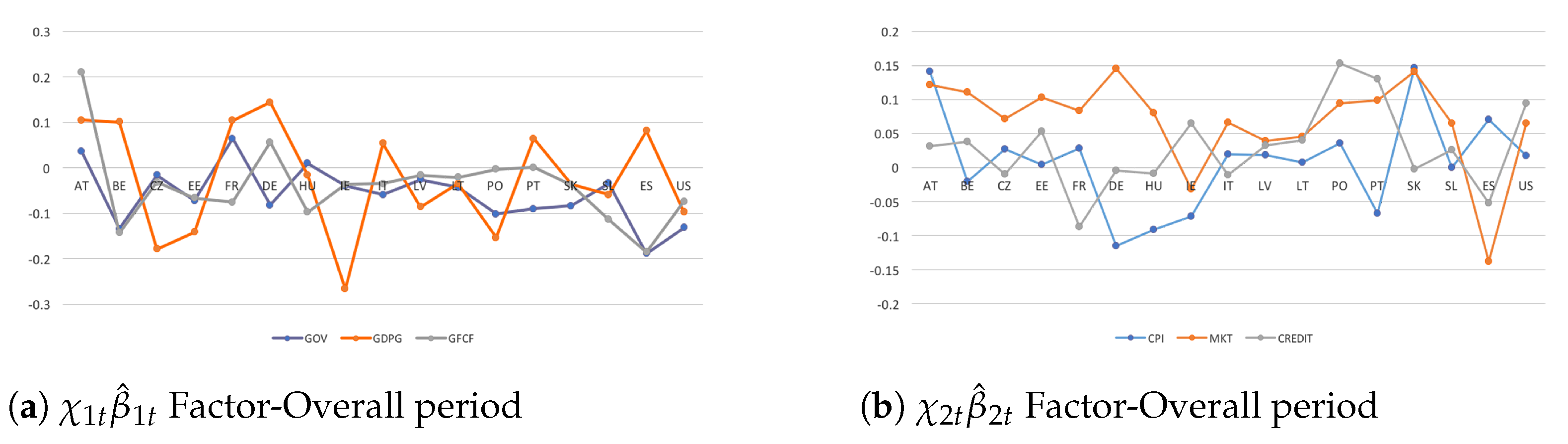
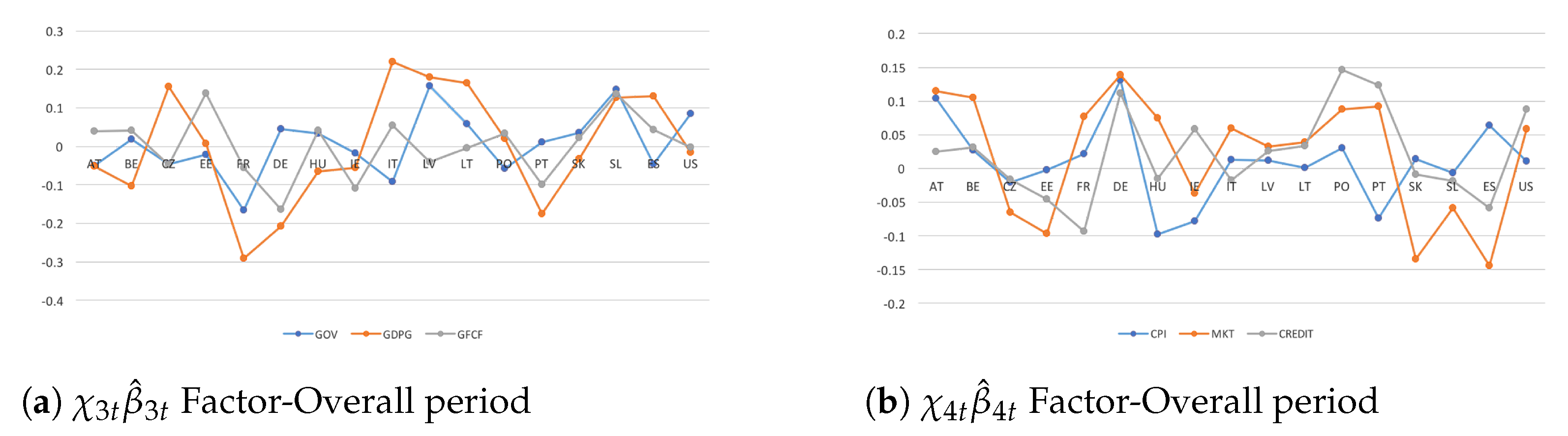
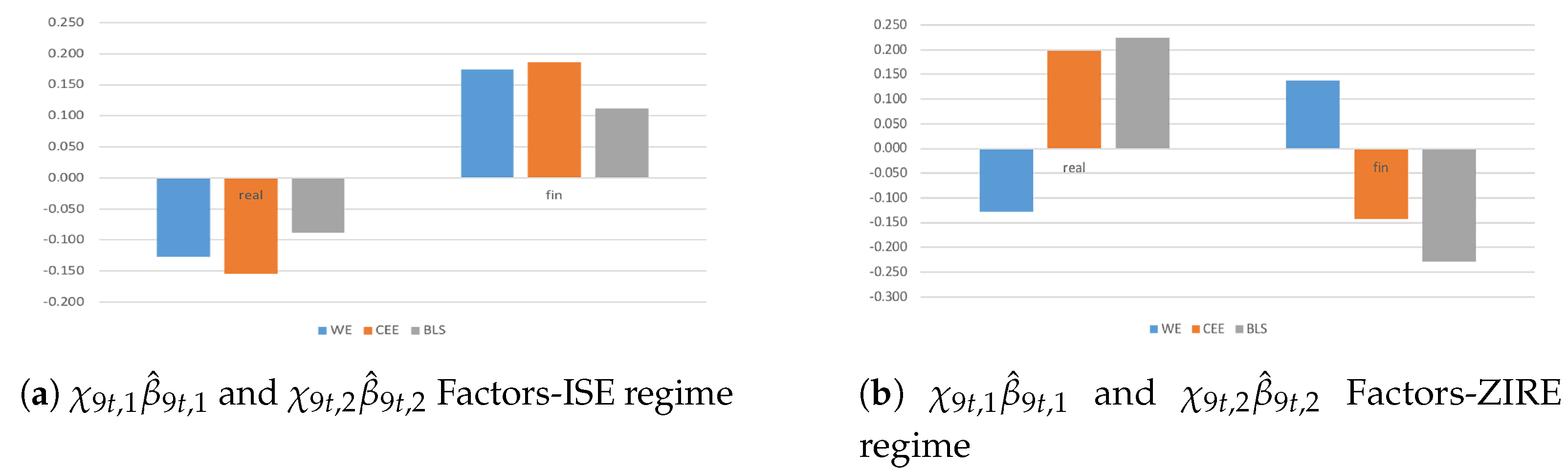
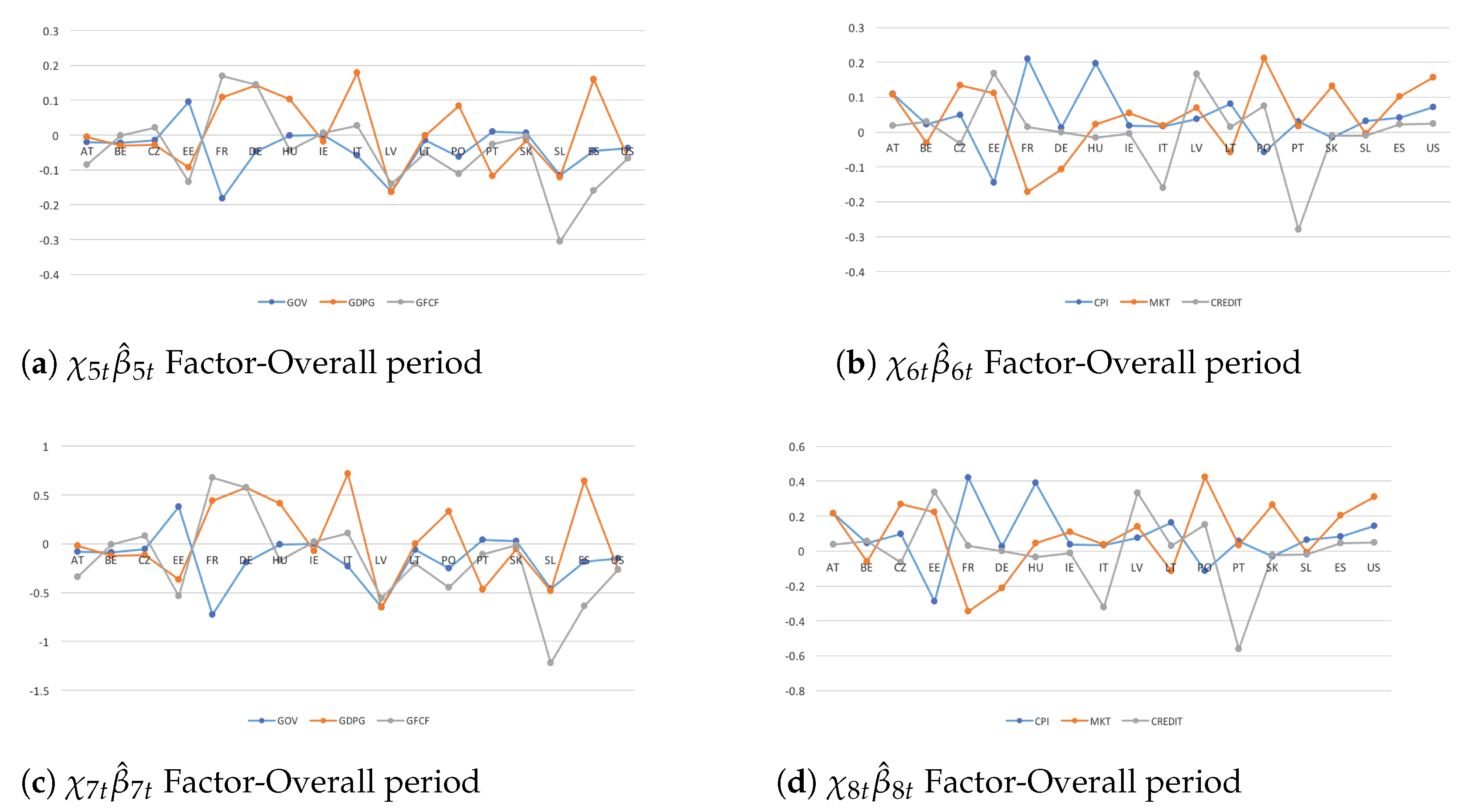
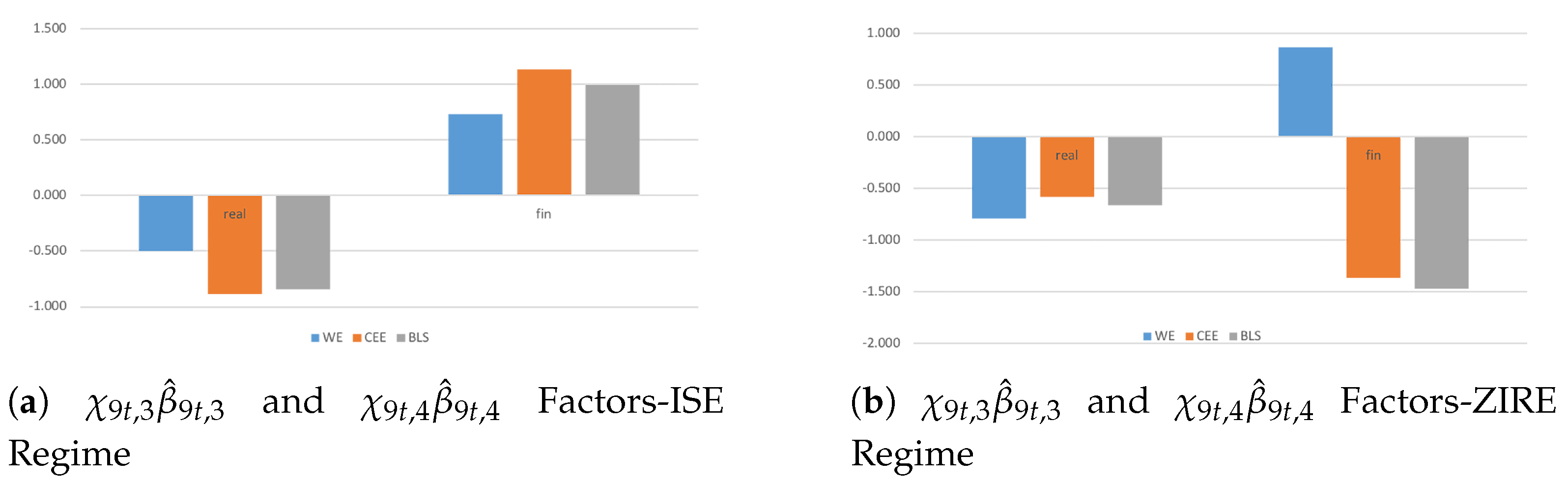
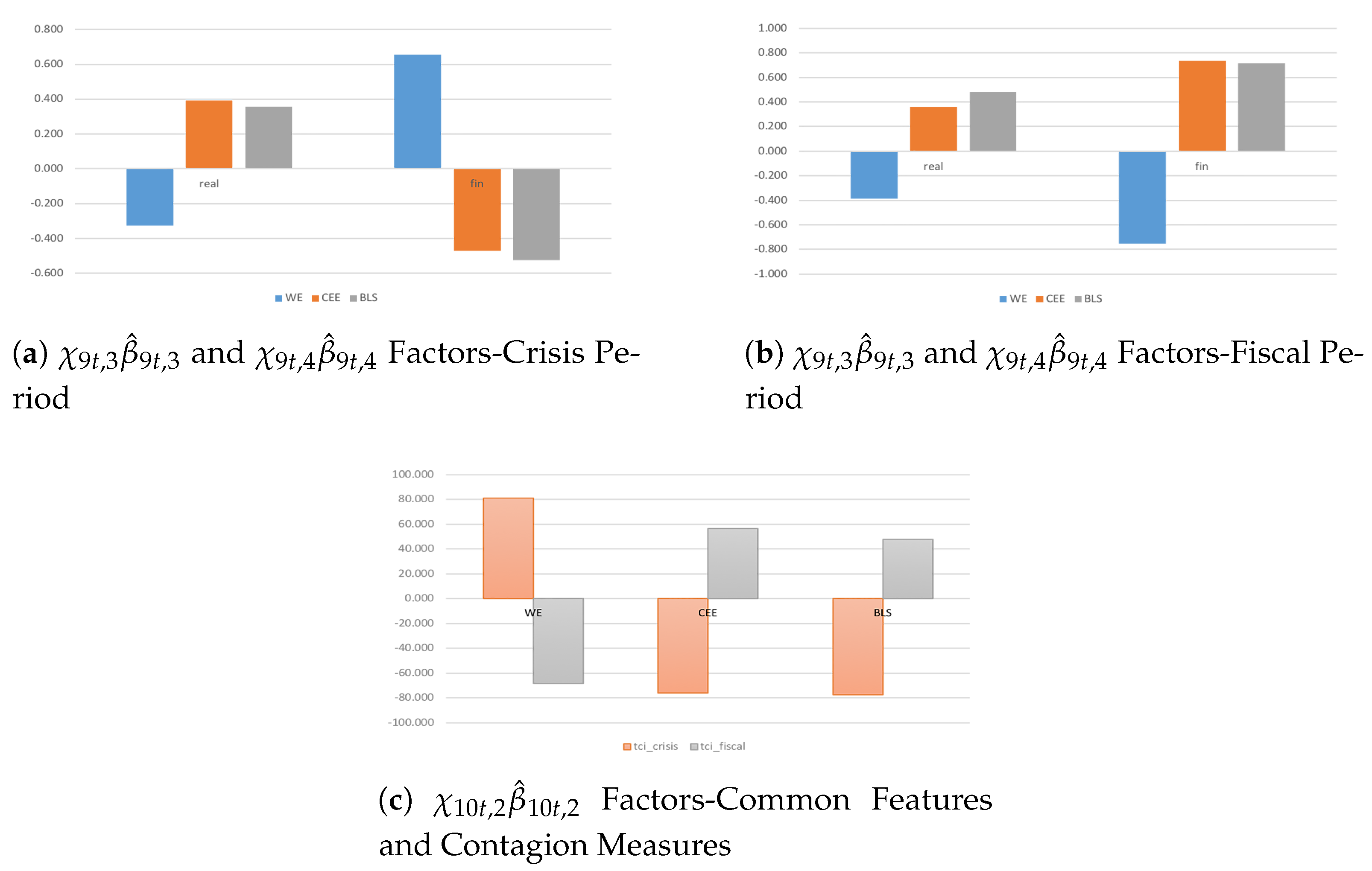
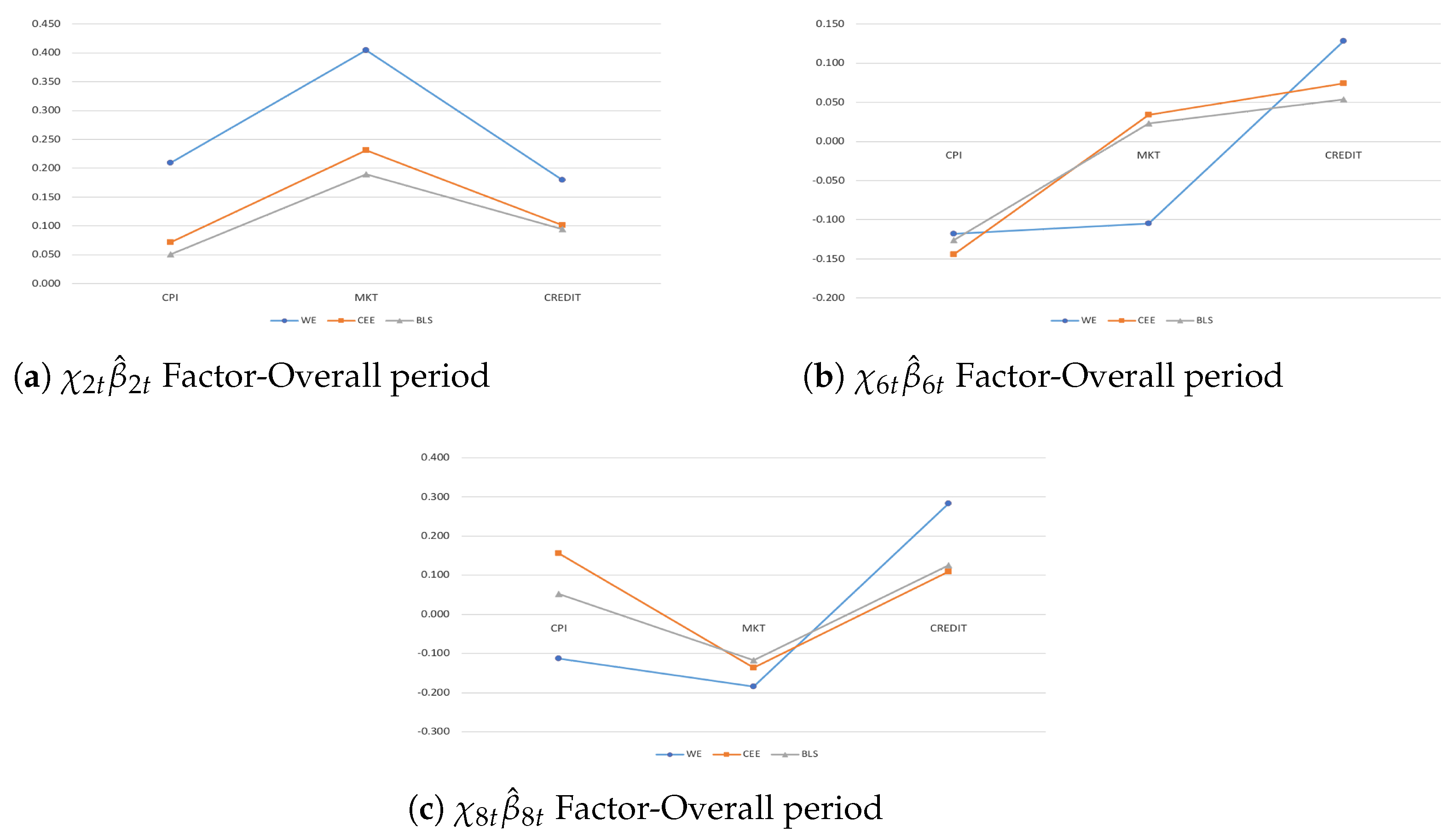
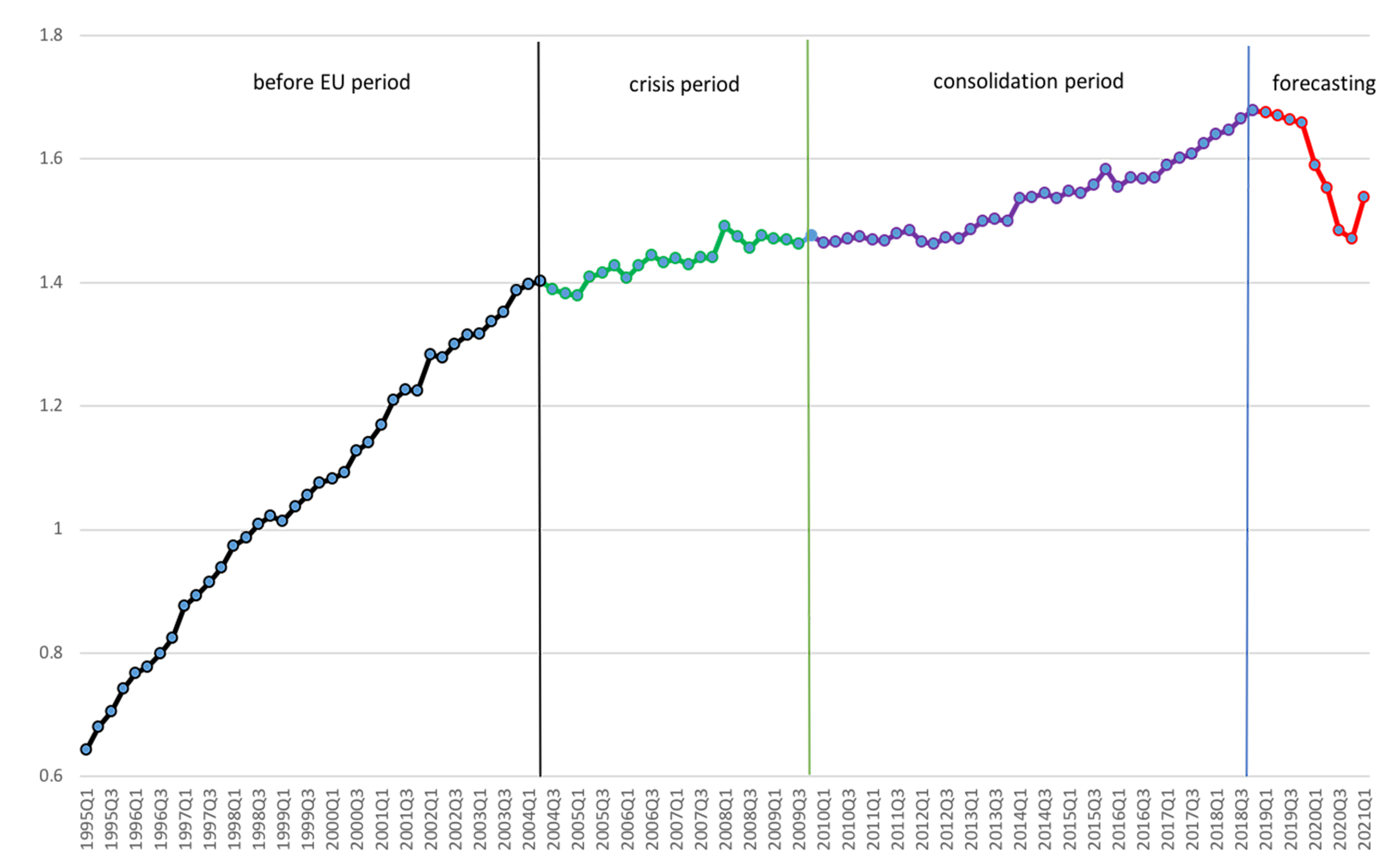
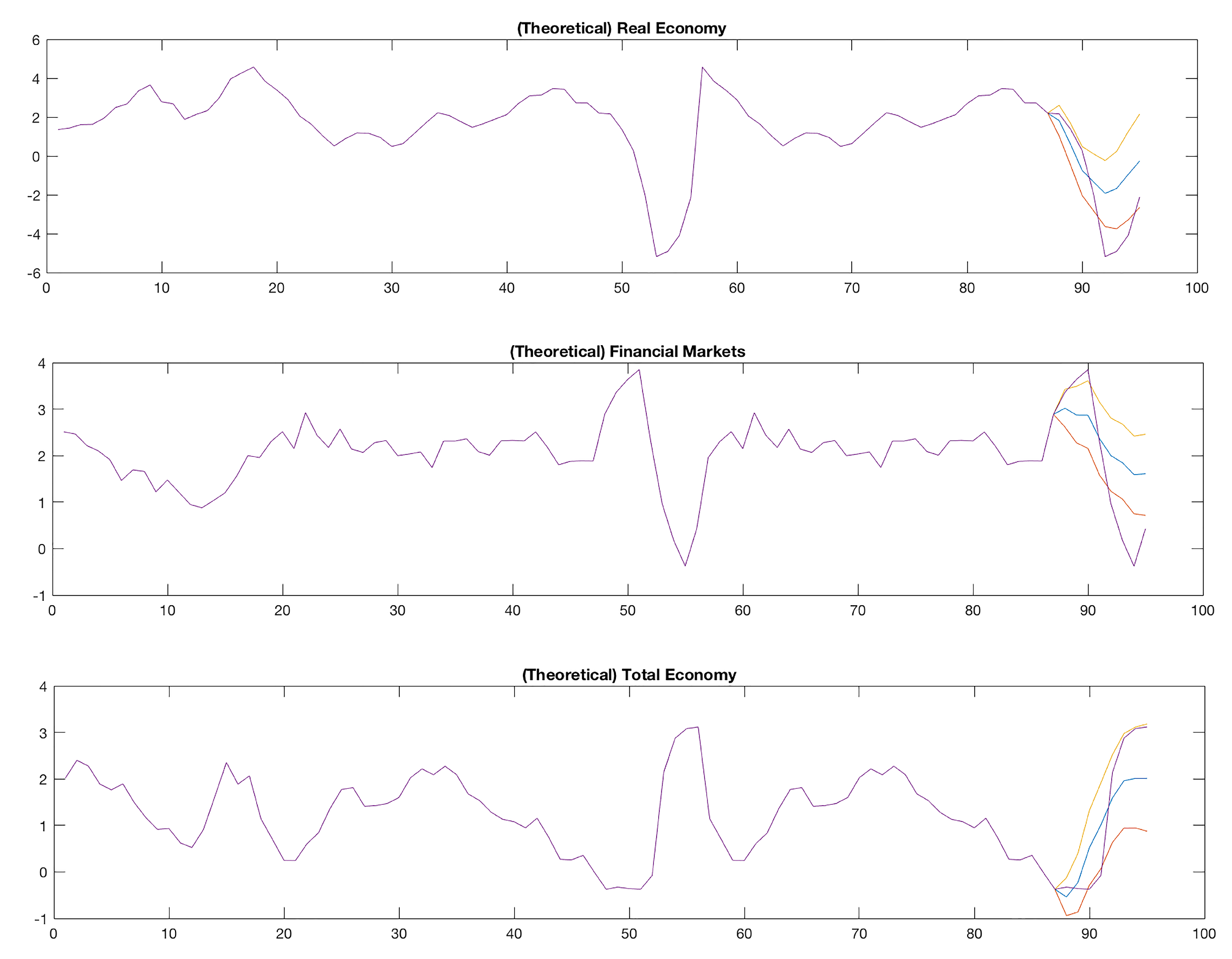
Table A1.
Data description.
| Variable | Data Description |
|---|---|
| General Government Spending | Financial accounts for general government spending. |
| Gross Fixed Capital Formation | Investments of fixed assets at current prices. |
| GDP Growth Rate | It is calculated as: . |
| Inflation | It is calculated from the Consumer Price Index. |
| Bank Leverage | It is calculated as Loan (L) to Deposit (D) ratio. |
| Credit Growth | It is calculated as: . |
| Bilateral Flows of Trade | Exports and imports in goods and services. |
| Financial Transactions | Financial Assets on the total economy. |
| Interest Rate | International interest policy rate. |
| Public Debt | Non-financial accounts for general government debt. |
| Current Account Balance | Non-financial accounts for general government net. |
| Financial Consumption Expenditure | Total general government expenditure at current prices. |
| Private Sector Consumption | Private consumption expenditure. |
| Change of Unemployment Rate | Growth rate of the unemployment rate as percentage. |
| Nominal Labour Cost | It is defined as the ratio of labour costs to labour productivity. |
| Household price index | Real household per capita index. |
| Productivity | It corresponds to logarithm of the real GDP per capita. |
| Here, general government spending, gross fixed capital formation, bilateral flows of trade, financial transactions, public debt, current account balance, financial consumption, private consumption, and unemployment rate are weighted for the GDP. | |
| 1. | |
| 2. | |
| 3. | See, for instance, Gelfand and Dey (1994). |
| 4. | It would correspond to the conditional density of the data given the log-volatilities, but marginal of the time-varying parameters. |
| 5. | Overfitting and thus overestimation of effect sizes refers to a common problem in Bayesian Model Averaging since more complex models will always provide a somewhat better fit to the data than simpler models, where the ’complexity’ stands (for example) for the number of unknown parameters. See, for instance, Pacifico (2020b). |
| 6. | |
| 7. | A proxy variable is an easily measurable variable used in place of a variable that cannot be directly measured. |
| 8. | |
| 9. | The vec operator transforms a matrix into a vector by stacking the columns of the matrix, one underneath the other. |
| 10. | Its form would be similar to the parsimonious Seemingly Unrelated Regression (SUR) model (homoskedastic VAR) developed in the literature (see, for instance, Canova and Ciccarelli (2009) and Ciccarelli et al. (2018)), but adapted to a hierarchical time-varying multicountry structural setup. |
| 11. | The Wishart distribution is a multivariate extension of distribution and, in Bayesian statistics, corresponds to the conjugate prior of the inverse covariance-matrix of a multivariate normal random vector. |
| 12. | They denote both unobserved heterogeneity and misspecification problems. |
| 13. | See Section 3.2 for further detail. |
| 14. | |
| 15. | |
| 16. | |
| 17. | See, for instance, Levine and Casella (2014). |
| 18. | Analytical integration for integrating out the time-varying log-volatilities are explained in depth in Section 3.2. |
| 19. | See, for instance, Carter and Kohn (1994). |
| 20. | See Section 4 for the form of the ’s and the ’s. |
| 21. | See Section 3.2.2. |
| 22. | See Section 3.3. |
| 23. | See, for instance, Jacquier et al. (2002). |
| 24. | See, for instance, Roberts and Rosenthal (2001). |
| 25. | |
| 26. | See, for instance, Kroese et al. (2011). |
| 27. | Czech Republic (CZ), Hungary (HU), Estonia (EE), Latvia (LV), Lithuania (LT), Poland (PO), Slovak Republic (SK), and Slovenia (SL). |
| 28. | Austria (AT), Belgium (BE), France (FR), Germany (DE), Ireland (IE), Italy (IT), Portugal (PT), and Spain (ES). |
| 29. | The component corresponds to the sum of and . |
| 30. | It stands for the Baltic States (EE, LV, and LT). |
| 31. | They refer to the advanced and then WE countries. |
| 32. | World Health Organization, 11 March 2020. |
| 33. | See, e.g., Dell’Ariccia et al. (2018); Guerrieri et al. (2020); Romer and Romer (2018), and Bernanke (2020). |
| 34. | See, e.g., Banbura et al. (2010); Carriero et al. (2015); Giannone et al. (2015), and Koop (2013) for recent studies on LBVAR models and time variation in their volatilities; and Clark (2011); Clark and Ravazzolo (2015a), and Primiceri (2005) concerning studies on the importance of time variation in the volatilities modeled as stochastic volatility. |
| 35. | Monte Carlo simulations would work well up to 35,000 data. Compared to higher sample (≥35,000), the associated computational costs seem to become quite expensive. In that case, whether one would be interested to improve the empirical analysis accounting for larger country indices and sets of variables, but ensuring consistent posterior estimates, a simple solution would be fixing the time (T) as necessary (e.g., according to the economic–financial and policy issues to be addressed). |
| 36. | The idea is to highlight the performance of the estimation method by conducting a simulated experiment preserving the empirical findings (such as presence of cross-unit interdependencies, commonality, and dynamic feedback and interactions related to (theoretical) unobserved effects). |
| 37. | The convergence has been found by amounting to about 1.5 draws per (theoretical) regression parameter. |
| 38. | Generally, the conditional projection in density forecasts is the one that the model would have obtained over the same period conditionally on the actual path of unexpected dynamics for that period. |
| 39. | Generally, the unconditional projection in density forecasts is the one that the model would obtain for output growth for that period only on the basis of historical information, and it is consistent with a model-based forecast path for the other variables. |
References
- Banbura, Marta, Domenico Giannone, and Lucrezia Reichlin. 2010. Large bayesian vector autoregressions. Journal of Applied Econometrics 25: 71–92. [Google Scholar] [CrossRef]
- Bernanke, Ben S. 2020. The new tools of monetary policy. American Economic Review 110: 943–83. [Google Scholar] [CrossRef] [Green Version]
- Canova, Fabio, and Matteo Ciccarelli. 2009. Estimating multicountry var models. International Economic Review 50: 929–59. [Google Scholar] [CrossRef] [Green Version]
- Canova, Fabio, Matteo Ciccarelli, and Eva Ortega. 2007. Similarities and convergence in g7 cycles. Journal of Monetary Economics 54: 850–78. [Google Scholar] [CrossRef] [Green Version]
- Canova, Fabio, Matteo Ciccarelli, and Eva Ortega. 2012. Do institutional changes affect business cycles? Journal of Economic Dynamics and Control 36: 1520–33. [Google Scholar] [CrossRef] [Green Version]
- Canova, Fabio, and Luca Gambetti. 2009. Structural changes in the us economy: Is there a role for monetary policy? Journal of Economic Dynamics and Control 33: 477–90. [Google Scholar] [CrossRef] [Green Version]
- Carriero, Andrea, Todd E. Clark, and Massimiliano Marcellino. 2015. Bayesian vars: specification choices and forecast accuracy. Journal of Applied Econometrics 30: 46–73. [Google Scholar] [CrossRef]
- Carriero, Andrea, Todd E. Clark, and Massimiliano Marcellino. 2019. Large bayesian vector autoregressions with stochastic volatility and non-conjugate priors. Journal of Econometrics 212: 137–54. [Google Scholar] [CrossRef]
- Carter, Chris K., and Robert Kohn. 1994. On gibbs sampling for state space models. Biometrika 81: 541–53. [Google Scholar] [CrossRef]
- Cette, Gilbert, John Fernald, and Benoît Mojon. 2016. The pre-great recession slowdown in productivity. European Economic Review 88: 3–20. [Google Scholar] [CrossRef] [Green Version]
- Chan, Joshua C. C., and Angelia L. Grant. 2015. Pitfalls of estimating the marginal likelihood using the modified harmonic mean. Economics Letters 131: 29–33. [Google Scholar] [CrossRef]
- Chan, Joshua C. C., and Ivan Jeliazkov. 2009. Efficient simulation and integrated likelihood estimation in state space models. International Journal of Mathematical Modelling and Numerical Optimisation 1: 101–20. [Google Scholar] [CrossRef]
- Ciccarelli, Matteo, Eva Ortega, and Maria T. Valderrama. 2018. Commonalities and cross-country spillovers in macroeconomic-financial linkages. Journal of Macroeconomics 16: 231–75. [Google Scholar] [CrossRef]
- Clark, Todd E. 2009. Is the great moderation over? an empirical analysis. Economic Review 94: 5–42. [Google Scholar]
- Clark, Todd E. 2011. Real-time density forecasts from bayesian vector autoregressions with stochastic volatility. Journal of Business and Economic Statistics 29: 327–41. [Google Scholar] [CrossRef]
- Clark, Todd E., and Francesco Ravazzolo. 2015. Macroeconomic forecasting performance under alternative specifications of time-varying volatility. Journal of Applied Econometrics 30: 551–75. [Google Scholar] [CrossRef]
- Cogley, Timothy, Giorgio E. Primiceri, and Thomas J. Sargent. 2010. Inflation-gap persistence in the us. American Economic Journal: Macroeconomic 2: 43–69. [Google Scholar] [CrossRef] [Green Version]
- Cogley, Timothy, and Thomas J. Sargent. 2005. Drifts and volatilities: Monetary policy and outcomes in the post wwii u.s. Review of Economic Dynamics 8: 262–302. [Google Scholar] [CrossRef] [Green Version]
- Coibion, Olivier, and Yuriy Gorodnichenko. 2012. Why are target interest rate changes so persistent? American Economic Journal: Macroeconomics 4: 126–62. [Google Scholar] [CrossRef] [Green Version]
- Curcio, Domenico, Rosa Cocozza, and Antonio Pacifico. 2020. Do global markets imply common fear? Rivista Bancaria-Minerva Bancaria 2020: 1–24. [Google Scholar]
- D’Agostino, Antonello, Luca Gambetti, and Domenico Giannone. 2013. Macroeconomic forecasting and structural change. Journal of Applied Econometrics 28: 82–101. [Google Scholar] [CrossRef] [Green Version]
- Daly, Mary C., John G. Fernald, Óscar Jordá, and Fernanda Nechio. 2016. Shocks and Adjustments. Working Paper 2013-32. San Francisco: Federal Reserve Bank of San Francisco. [Google Scholar]
- Dell’Ariccia, Giovanni, Pau Rabanal, and Damiano Sandri. 2018. Unconventional monetary policies in the euro area, japan, and the united kingdom. Journal of Economic Perspectives 32: 147–72. [Google Scholar] [CrossRef] [Green Version]
- Foerster, Andrew, and Christian Matthes. 2020. Learning about Regime Change. Working Paper 2020-15. San Francisco: Federal Reserve Bank of San Francisco. [Google Scholar]
- Frühwirth-Schnatter, Sylvia, and Helga Wagner. 2008. Marginal likelihoods for non-gaussian models using auxiliary mixture sampling. Computational Statistics and Data Analysis 52: 4608–24. [Google Scholar] [CrossRef]
- Gelfand, Alan E., and Dipak K. Dey. 1994. Bayesian model choice: Asymptotics and exact calculations. Journal of the Royal Statistical Society: Series B 56: 501–14. [Google Scholar]
- Giannone, Domenico, Michele Lenza, and Giorgio E. Primiceri. 2015. Prior selection for vector autoregressions. The Review of Economics and Statistics 97: 436–51. [Google Scholar] [CrossRef] [Green Version]
- Guerrieri, Veronica, Guido Lorenzoni, Ludwig Straub, and Iván Werning. 2020. Macroeconomic Implications of covid-19: Can Negative Supply Shocks Cause Demand Shortages? NBER Working Paper 26918. Cambridge: National Bureau of Economic Research. [Google Scholar]
- Jacquier, Eric, Nicholas G. Polson, and Peter E. Rossi. 2002. Bayesian analysis of stochastic volatility. Journal of Business and Economic Statistics 20: 69–87. [Google Scholar] [CrossRef]
- Kadiyala, Rao K., and Sune Karlsson. 1997. Numerical methods for estimation and inference in bayesian var models. Journal of Applied Econometrics 12: 99–132. [Google Scholar] [CrossRef]
- Kallianiotis, Ioannis N. 2019. Monetary policy, real cost of capital, financial markets and the real economic growth. Journal of Applied Finance & Banking 9: 75–118. [Google Scholar]
- Kass, Robert E., and Adrian E. Raftery. 1995. Bayes factors. Journal of American Statistical Association 90: 773–95. [Google Scholar] [CrossRef]
- Koop, Gary. 1996. Parameter uncertainty and impulse response analysis. Journal of Econometrics 72: 135–49. [Google Scholar] [CrossRef]
- Koop, Gary. 2013. Forecasting with medium and large bayesian vars. Journal of Applied Econometrics 28: 177–203. [Google Scholar] [CrossRef] [Green Version]
- Koop, Gary, and Dimitris Korobilis. 2016. Model uncertainty in panel vector autoregressive models. European Economic Review 81: 115–31. [Google Scholar] [CrossRef] [Green Version]
- Koop, Gary, Roberto Leon-Gonzalez, and Rodney W. Strachan. 2009. On the evolution of the monetary policy transmission mechanism. Journal of Economic Dynamics and Control 33: 997–1017. [Google Scholar] [CrossRef]
- Korobilis, Dimitris. 2016. Prior selection for panel vector autoregressions. Computational Statistics and Data Analysis 101: 110–20. [Google Scholar] [CrossRef] [Green Version]
- Kroese, Dirk P., and Joshua C. C. Chan. 2014. Statistical Modeling and Computation. New York: Springer. [Google Scholar]
- Kroese, Dirk P., Thomas Taimre, and Zdravko I. Botev. 2011. Handbook of Monte Carlo Methods. New York: John Wiley and Sons. [Google Scholar]
- Krolzig, Hans-Martin. 1997. Markov Switching Vector Autoregressions: Modelling, Statistical Inference and Application to Business Cycle Analysis. Berlin: Springer. [Google Scholar]
- Krolzig, Hans-Martin. 2000. Predicting Markov-Switching Vector Autoregressive Processes. Nuffield College Economics Working Papers, 2000-WP31. Oxford: Nuffield College. [Google Scholar]
- Levine, Richard A., and George Casella. 2014. Implementations of the monte carlo em algorithm. Journal of Computational and Graphical Statistics 10: 422–39. [Google Scholar] [CrossRef] [Green Version]
- Liu, Yuelin, and James Morley. 2014. Structural evolution of the u.s. economy. Journal of Economic Dynamics and Control 42: 50–68. [Google Scholar] [CrossRef] [Green Version]
- McLachlan, Geoffrey J., Thriyambakam Krishnan, and Shu K. Ng. 2012. The em Algorithm. Handbook of Computational Statistics. Berlin and Heidelberg: Springer. [Google Scholar]
- Pacifico, Antonio. 2019a. International co-movements and business cycles synchronization across advanced economies: A spbvar evidence. International Journal of Statistics and Probability 8: 68–85. [Google Scholar] [CrossRef]
- Pacifico, Antonio. 2019b. Structural panel bayesian var model to deal with model misspecification and unobserved heterogeneity problems. Econometrics 7: 1–24. [Google Scholar] [CrossRef] [Green Version]
- Pacifico, Antonio. 2020a. Fiscal implications, misspecified dynamics, and international spillover effects across europe: A time-varying multicountry analysis. International Journal of Statistics and Economics 21: 18–40. [Google Scholar]
- Pacifico, Antonio. 2020b. Robust open bayesian analysis: Overfitting, model uncertainty, and endogeneity issues in multiple regression models. Econometric Reviews 40: 148–76. [Google Scholar] [CrossRef]
- Primiceri, Giorgio E. 2005. Time varying structural vector autoregressions and monetary policy. Review of Economic Studies 72: 821–52. [Google Scholar] [CrossRef]
- Roberts, Gareth O., and Jeffrey S. Rosenthal. 2001. Optimal scaling for various metropolis-hastings algorithms. Statistical Science 16: 351–67. [Google Scholar] [CrossRef]
- Romer, Christina D., and David H. Romer. 2018. Phillips lecture-why some times are different: macroeconomic policy and the aftermath of financial crises. Economica 85: 1–40. [Google Scholar] [CrossRef]
- Sims, Christopher A., and Tao Zha. 2006. Were there regime switches in u.s. monetary policy? The American Economic Review 96: 54–81. [Google Scholar] [CrossRef] [Green Version]
- Steele, Brian M. 1996. A modified em algorithm for estimation in generalized mixed models. Biometrics 52: 1295–310. [Google Scholar] [CrossRef] [PubMed]
- Stock, James H., and Mark W. Watson. 2012. Disentangling the Channels of the 2007–2009 Recession. NBER Working Paper Series. Cambridge: National Bureau of Economic Research, vol. 18094. [Google Scholar]
- Tjalling, Ypma J. 1995. Historical development of the newton-raphson method. SIAM Review 37: 531–51. [Google Scholar]
Figure 1.
Systemic contributions of the productivity given a shock to real and financial dimensions are drawn as standard deviations of the variables in the system. They account for (plot a) and (plot b) cross-country indicators, where and are posterior means.
Figure 1.
Systemic contributions of the productivity given a shock to real and financial dimensions are drawn as standard deviations of the variables in the system. They account for (plot a) and (plot b) cross-country indicators, where and are posterior means.

Figure 2.
Systemic contributions of the given a shock to real and financial dimensions are drawn as standard deviations of the variables in the system. They account for (plot a) and (plot b) cross-country indicators, where and are posterior means.
Figure 2.
Systemic contributions of the given a shock to real and financial dimensions are drawn as standard deviations of the variables in the system. They account for (plot a) and (plot b) cross-country indicators, where and are posterior means.

Figure 3.
Systemic contributions of the productivity given a shock to real and financial dimensions are drawn as standard deviations of the variables in the system. They account for the variable-specific indicators and during ISE (plot a) and ZIRE (plot b) regimes, where ’s are posterior means with .

Figure 4.
Systemic contributions of the productivity given a shock to real and financial dimensions are drawn as standard deviations of the variables in the system. They account for the cross-country indicators (plot a), (plot b), (plot c), and (plot d), where , , , and are posterior means.
Figure 4.
Systemic contributions of the productivity given a shock to real and financial dimensions are drawn as standard deviations of the variables in the system. They account for the cross-country indicators (plot a), (plot b), (plot c), and (plot d), where , , , and are posterior means.

Figure 5.
Systemic contributions of the productivity given a shock to real and financial dimensions are drawn as standard deviations of the variables in the system. They account for the variable-specific indicators and during ISE (plot a) and ZIRE (plot b) regimes, where ’s are posterior means with .

Figure 6.
Systemic contributions of the productivity given a shock to real and financial dimensions are drawn as standard deviations of the variables in the system. They account for the variable-specific indicators and during crisis (plot a) and post-crisis (plot b) periods, where ’s are posterior means with .

Figure 7.
Systemic contributions of the productivity given a shock to financial markets are drawn as standard deviations of the variables in the system. They account for the cross-country indicators (plot a), (plot b), and (plot c), where , , and are posterior means.
Figure 7.
Systemic contributions of the productivity given a shock to financial markets are drawn as standard deviations of the variables in the system. They account for the cross-country indicators (plot a), (plot b), and (plot c), where , , and are posterior means.

Figure 8.
Generalized Entropy index according to the productivity growth from to is drawn. It corresponds to the Theil’s Entropy and is computed by weighing the GDP with the population in terms of proportions with respect to the total. The conditional projections of each variable drawn in the SPBVAR-MTV in (1) have been used to perform forecasting from to .

Figure 9.
The plot draws (theoretical) density forecast combinations for outcomes given N for the indicators that account for additional factors and policy shifts with unobserved effects. They are: (’theoretical’ real economy); (’theoretical’ financial markets); and (’theoretical’ total economy). They correspond to (theoretical) conditional (blue line) and unconditional (purple line) projections of each supposed variable drawn in (82).

Table 1.
Diagnostic Tests.
| Test | Test Statistics | Degrees of Freedom | p-Value |
|---|---|---|---|
| 16573 | 1649 | 0.00 | |
| 837.3 | 1261 | 0.30 | |
| 67.44 | 10 | 0.00 |
Here, LGBπ stands for a Multivariate Ljung-Box Test of the series, with lags π = 30; Pπ refers to the Portmanteau (Asymptotic) Test on the residuals, with lags π = 30; MLEf is the Marginal (Conditional) Likelihood Estimation Test obtained through the Schwartz approximation, with f = 10.
Table 2.
Empirical results on the benchmark model.
| Time-Varying Factors | ‘General Case’ () | ‘Special Case’ () | ‘Full Case’ () |
|---|---|---|---|
| lBF >10 | |||
| lBF >10 | |||
| lBF >10 | |||
| lBF >10 | |||
| lBF >10 | |||
| lBF >10 | |||
| lBF >10 | |||
| lBF >10 |
The first column denotes the time-varying factors and the other three columns refer to all three (potential) best benchmark models. The best model solution is highlithed in bold and corresponds to the highest log Bayes Factor according to the generalized version of the Kass and Raftery (1995)’s scale of evidence in (53).
Table 3.
Simulated experiments.
| Theoretical Factors | General Case () | Full Case () | |||
|---|---|---|---|---|---|
| BVAR | PBVAR | SPBVAR | LBVAR-SV | SPBVAR-MTV | |
| 0.062 * | 0.058 * | 0.023 ** | 0.026 ** | 0.022 ** | |
| 0.052 * | 0.047 ** | 0.022 ** | 0.021 ** | 0.018 ** | |
| 0.214 | 0.145 | 0.057 * | 0.015 ** | 0.009 *** | |
| 0.112 | 0.131 | 0.044 ** | 0.028 ** | 0.017 ** | |
| 0.301 | 0.225 | 0.051 * | 0.015 ** | 0.007 *** | |
| 0.201 | 0.173 | 0.057 * | 0.031 ** | 0.012 ** | |
| 0.034 ** | 0.031 ** | 0.010 ** | 0.006 *** | 0.003 *** | |
| 0.093 * | 0.076 * | 0.042 ** | 0.012 ** | 0.008 *** | |
| 0.307 | 0.214 | 0.107 | 0.092 * | 0.021** | |
The first column denotes the time-varying (theoretical) factors and the remaining columns refer to the (theoretical) posterior estimates (in p-values) obtained for all five supposed Bayesian approaches according to the competing models MI and MIII. The best model solution accounts for the only (theoretical) factors highlighted in bold and corresponds to the highest log Bayes Factor (lBF > 10) according to the generalized version of the Kass and Raftery (1995)’s scale of evidence in (53). The significance codes stand for: (*) significance at 10%; (**) significance at 5%; and (***) significance at 1%.
Publisher’s Note: MDPI stays neutral with regard to jurisdictional claims in published maps and institutional affiliations. |
© 2021 by the author. Licensee MDPI, Basel, Switzerland. This article is an open access article distributed under the terms and conditions of the Creative Commons Attribution (CC BY) license (https://creativecommons.org/licenses/by/4.0/).
Share and Cite
MDPI and ACS Style
Pacifico, A. Structural Panel Bayesian VAR with Multivariate Time-Varying Volatility to Jointly Deal with Structural Changes, Policy Regime Shifts, and Endogeneity Issues. Econometrics 2021, 9, 20. https://doi.org/10.3390/econometrics9020020
AMA Style
Pacifico A. Structural Panel Bayesian VAR with Multivariate Time-Varying Volatility to Jointly Deal with Structural Changes, Policy Regime Shifts, and Endogeneity Issues. Econometrics. 2021; 9(2):20. https://doi.org/10.3390/econometrics9020020
Chicago/Turabian StylePacifico, Antonio. 2021. "Structural Panel Bayesian VAR with Multivariate Time-Varying Volatility to Jointly Deal with Structural Changes, Policy Regime Shifts, and Endogeneity Issues" Econometrics 9, no. 2: 20. https://doi.org/10.3390/econometrics9020020
Note that from the first issue of 2016, this journal uses article numbers instead of page numbers. See further details here.