Estimating Ocean Surface Currents With Machine Learning

1. Introduction

The most reliable spatially continuous estimates of global surface currents in the ocean come from geostrophic balance applied to the sea surface height (SSH) field observed by satellite altimeters. For the most part, the dynamics of slow, large-scale currents (up to the mesoscale) are well-approximated by geostrophic balance, leading to a direct relationship between gradients of SSH and near-surface currents. However, current meter observations for the past few decades and some of the newer generation ultra-high-resolution numerical model simulations indicate the presence of an energized submesoscale as well as high-frequency waves/tides at smaller spatial and temporal scales (Rocha et al., 2016). In addition, the next generation of satellite altimeters like the upcoming Surface Water and Ocean Topography (SWOT) mission (Morrow et al., 2018) is going to capture the ocean surface at a much higher spatial resolution, but with a low frequency repeat cycle (21 days). This presents unique challenges for the estimation of surface currents from SSH using traditional balances like geostrophy or Ekman. The high-wavenumber SSH variability is likely to be strongly aliased in the temporally sub-sampled data and may represent an entirely different, ageostrophic regime, where geostrophy might not be the best route to infer velocities. Motivated by this problem, we explore statistical models based on machine learning (ML) algorithms for inferring surface currents from satellite observable quantities like SSH, wind and temperature in this study. These algorithms can offer a potential alternative to the traditional physics-based models. We should point out that resolving the issues pertaining to spatio-temporal sampling and interpolation in satellite altimetry or the separation of balanced and unbalanced flows, while being important problems, are beyond the scope of our present study. Our goal is to examine whether we can extract more information about the surface flow from the spatial maps of these quantities and make more accurate predictions of surface currents with ML than we can with traditional balances.

The traditional method of calculating surface currents from sea surface height relies on the following physical principles. Assuming 2D flow and shallow water pressure, the momentum equation at the ocean surface can be written as:

where F is the frictional term due to wind stress. For a sufficiently low Rossby number (acceleration terms small), the leading-order balances are geostrophy and Ekman flow. The surface flow can be split into a geostrophic and an ageostrophic, Ekman component (u = u_g + u_e), and this leading-order force balance can be written as

Satellite altimetery products typically provide the sea surface height relative to the geoid (SSH, η), with tidally driven SSH signals removed (Traon and Morrow, 2001). Since geostrophic balance does not hold at the equator (f ≈ 0), typically (Ducet et al., 2000), a higher order “equatorial geostrophic” treatment is used to compute velocities near the equator (Lagerloef et al., 1999), which is matched to the geostrophic regime away from the equator. Usually, the data-assimilative processing algorithms used to map along-track SSH observations to gridded maps (e.g., AVISO Ducet et al., 2000) also involve some form of temporal smoothing. The process of combining measurements from multiple satellites and filtering can also lead to spurious physical signals (Arbic et al., 2012) leading to exaggerated forward-cascades of energy.

In addition to the geostrophic velocities, some products like OSCAR (Ocean Surface Current Analysis Real Time, Bonjean and Lagerloef, 2002), or GEKCO (Geostrophic and Ekman Current Observatory, Sudre and Morrow, 2008; Sudre et al., 2013) provide an additional ageostrophic component due to Ekman flow. The Ekman velocity is related to friction, which in the upper layer of the ocean is provided by wind stress (τ = (τ_x, τ_y)) and since the Coriolis parameter f changes sign at the equator, the functional relationship between velocity and wind stress is different between the two hemispheres. In the Northern Hemisphere the Ekman velocities can be derived as:

And in the Southern Hemisphere as:

where A_z is the linear drag coefficient representing vertical eddy viscosity ($\tau =\rho A_z\frac{\partial \text{u}}{\partial z}$). Alternatively we can write these equations in terms of the Ekman layer depth h_Ek which is related to the eddy viscosity A_z as:

Both of these quantities (A_z,h_Ek) are largely unknown for the global ocean and are estimated based on empirical multiple linear regression from Lagrangian surface drifters (Lagerloef et al., 1999; Sudre et al., 2013). Typical values of Ekman depth h_Ek in the ocean range from 10 to 40 m.

So geostrophy + Ekman is the essential underlying physical/dynamical “model” currently used for calculating surface currents from satellite observations. This procedure, combining observations with physical principles, represents a top-down approach A more bottom-up approach would be a data driven regression model that extracts information about empirical relationships from data. Recently, machine learning (ML) methods have grown in popularity and have been proposed for a wide range of problems in fluid dynamics: Reynolds-averaged turbulence models (Ling et al., 2016), detecting eddies from altimetric SSH fields (Lguensat et al., 2017), reconstructing subsurface flow-fields in the ocean from surface fields (Chapman and Charantonis, 2017; Bolton and Zanna, 2019), sub-gridscale modeling of PDEs (Bar-Sinai et al., 2018), predicting the evolution of large spatio-temporally chaotic dynamical systems (Pathak et al., 2018), data-driven equation discovery (Zanna and Bolton, 2020), parameterizing unresolved processes, like convective systems in climate models (Gentine et al., 2018), or eddy momentum fluxes in ocean models (Bolton and Zanna, 2019), to name just a few examples.

In this study we aim to tackle a simpler problem than those cited above: training a ML model to “learn” the empirical relationships between the different observable quantities (sea surface height, wind stress, etc.) and surface currents (u, v). The hypothesis to be tested is the following: Can we use machine learning to provide surface current estimates more accurately than geostrophy + Ekman balance? The motivation for doing this exercise is 2-fold:

1. It will help us understand how machine learning can be applied in the context of traditional physics-based theories. ML is often criticised as a “black box.” But can we use ML to complement our physical understanding? This present problem serves as a good test-bed since the corresponding physical model is straightforward and well-understood.

2. It may be of practical value when SWOT mission launches.

While statistical models can often be difficult to explain due to lack of simple intuitive physical interpretations, several recent publications (Ling et al., 2016; Gentine et al., 2018; Bolton and Zanna, 2019; Zanna and Bolton, 2020) have demonstrated that data-driven approaches, used concurrently with physics-based models can offer various computational advantages over traditional methods, while still respecting physical principles. For our problem, which is much simpler in terms of its scope, we aim to mitigate the so called “black-box” ness of statistical models in general with physically motivated choices about inputs and training strategies, to ensure results that are physically meaningful. In this study, we mainly explore two types of regression models (multiple linear regression and artificial neural networks) as potential alternative approaches for predicting surface currents, using data from a primitive equation global general circulation model, and discuss their relative strengths and weaknesses. We see this work as a stepping stone to more complex applications of ML to ocean remote sensing of ocean surface currents.

This paper is organized as follows. In section 2, we introduce the dataset that was used, the framework of the problem and identify the key variables that are required for training a statistical model to predict surface currents. In section 3 we describe numerical evaluation procedure for baseline physics-based model that we are hoping to match/beat. In sections 4 and 5 we discuss the statistical models that we used. We start with the simplest statistical model—linear regression in section 4 before moving on to more advanced methods like neural networks in section 5. In section 6 we compare the results from the different models. In section 7 we summarize the findings, discuss some of the shortcomings of the present approach, propose some solutions as well as outline some of the future goals for this project.

2. Dataset and Input Features

To focus on the physical problem of relating currents to surface quantities, rather than the observational problems of spatio-temporal sampling and instrument noise, we choose to analyze a high-resolution global general circulation model (GCM), which provides a fully sampled, noise-free realization of the ocean state. The dataset used for this present study is the surface fields from the ocean component of the Community Earth System Model (CESM), called the Parallel Ocean Program (POP) simulation (Smith et al., 2010) which has a ≈ 0.1° horizontal resolution, with daily-averaged outputs available for the surface fields. The model employs a B-grid (scalars at cell centers, vectors at cell corners) for the horizontal discretization and a three-time-level second-order-accurate modified leap-frog scheme for stepping forward in time. The model solves the primitive equations of motion, which, for the surface flow, are essentially (1). Further details about the model physics and simulations can be found in Small et al. (2014) and Uchida et al. (2017). We selected this particular model simulation because of the long time record of available data (~40 years), although, in retrospect, we found that all our ML models can be trained completely with just a few days of output!

A key choice in any ML application is the choice of features, or inputs, to the model. In this paper, we experiment with a range of different feature combinations; seeing which features are most useful for estimating currents is indeed one of our aims. The features we choose are all quantities that are observable from satellites: SSH, surface wind stress (τ_x and τ_y), sea-surface temperature (SST, θ) and sea-surface Salinity (SSS). Our choice of features is also motivated by the traditional physics-based model: the same information that goes into the physics-based model should also prove useful to the ML model. Just like the physics-based model, all the ML models we consider are pointwise, local models: the goal is to predict the 2D velocity vector u, v at each point, using data from at or around that point.

Beyond these observable physical quantities, we also need to provide the models with geographic information about the location and spacing between the neighboring points. In the physics-based model, geography enters in two places: (1) in the Coriolis parameter f, and (2) in the grid spacing dx and dx, which varies over the model domain. Geographic information can be provided to the statistical models in a few different ways. The first method involves providing the same kind of spatial information that is provided to the physical models, i.e., f and local grid spacings—dx and dy. We can also encode geographic information (lat, lon) in our input features, using a coordinate transformation of the form:

to transform the spherical polar lat-lon coordinate into a homogeneous three dimensional coordinate (Gregor et al., 2017). This transformation gives the 3D position of each point in Euclidean space, rather than the geometrically warped lat/lon space (which has a singularity at the poles and a discontinuity at the dateline). Note that one of the coordinates—X, that comes out of this kind of coordinate transformation, is functionally the same as the Coriolis parameter (f) normalized by 2Ω (Ω = Earth's rotation). Therefore, we will use X as proxy for f for all the statistical models throughout this study. We also explored another approach where the only geographic information provided to the models is X ($=\frac{f}{2\Omega }$).

Since geostrophic balance involves spatial derivatives, it is not sufficient to simply provide SSH and the local coordinates pointwise. In order to compute derivatives, we also need the SSH of the surrounding grid points as a local stencil around each grid point. The approach we used for providing this local stencil is motivated by the horizontal discretization of the POP model. Horizontal derivatives of scalars (like SSH) on the B grid requires four cell centers. At every timestep, each variable of the The 1° POP model ouput has 3, 600 × 2, 400 data points (minus the land mask). We can simply rearrange each variable as a 1, 800 × 1, 200 × 2 × 2 dataset or split it into four variables each with 1, 800 × 1, 200 data points, corresponding to the four grid cells required for taking spatial derivatives. The variables that require a spatial stencil for physical models, we will refer to as the stencil inputs. For the variables for which we do not need spatial derivatives for (like wind stress), we can simply use every alternate grid point resulting in a dataset of size 1, 800 × 1, 200. We will refer to these variables as point inputs. For the purpose of the statistical models the inputs need to be flattened and have all the land points removed. This means that each input variable has a shape of either N × 2 × 2 or N depending on whether or not a spatial stencil is used (where N = 1, 800 × 1, 200−the points that fall over land). Alternatively we can think of the stencilled variable as four features of length N. This kind of stencil essentially coarsens the resolution of the targets, and point variables. Similarly we can also construct a three point time stencil, by providing the values at preceding and succeeding time steps as additional inputs so that each variable that is stencilled in space and time has a shape of N × 2 × 2 × 3 (or 12 features of length N). This data preparation leads to 10 potential features (for some of which we will use a stencil, which further expands the feature vector space) for predicting u, v at each point : τ_x, τ_y, SSH (η), SST (θ), SSS (S), the three transformed coordinates (X,Y,Z) and the local grid spacings (dx and dy).

For building any statistical/ML model, we need to split the dataset into two main parts, i.e., training and testing. For the purpose of training our machine learning models, the first step involves extracting the above mentioned variables from the GCM output as the input features and the GCM output surface velocities u, v as targets for the ML model. The data extracted from the GCM output for a certain date (or range of dates) is then used to fit the model parameters. This part of the dataset is called the training dataset. During training, the model minimizes a chosen cost function (we used mean absolute error for our experiments, but using mean squared error produced very similar results) and typically involves a few passes through this section of dataset. The trained models are then used to make predictions of u, v for a different date (or range of dates) where the model only receives the input variables. The model predictions are evaluated by comparing with the true (GCM output) velocity fields for that particular date (date range). This part of the dataset, which the model has not seen during training, that is used to evaluate model predictions is called the test dataset.

3. Baseline Physics-Based Model: Geostrophy + Ekman

The two components of the physics-based model used as the baseline for our ML models are geostrophy and Ekman flow. In this section we describe how these two components are numerically evaluated for our dataset. For the sake of fair comparison, we evaluate the geostrophic and Ekman velocities from the same features that are provided to the regression models. With the POP model's horizontal discretization, finite-difference horizontal derivatives and averages are defined as (Smith et al., 2010):

With the data preparation and stencil approach described in the previous section, η now has a shape of N × 2 × 2 and the f, u, v, dx, dy are all variables of length N. Following (2) the geostrophic velocities ($u_g^j,v_g^j$) are calculated on the stencil as:

where j ∈ [1, N]. Similarly the Ekman velocity is calculated numerically from the ${\tau }_x^j,{\tau }_y^j$, and f^j as

For calculating the Ekman velocity, we used constant values for vertical diffusivity ($A_z=8\times 10^{-3}{m}^2/s$) and density of water at the surface (ρ = 1, 027kg/m³). It should be noted that both these quantities vary both spatially and temporally in the real ocean. For the vertical diffusivity we came up with this estimate by solving for A_z that provides the best fit between zonal mean ((u, v)_true − (u, v)_g) and (u, v)_e. In the CESM high res POP simulations, the parameterized vertical diffusivity was capped around 100 cm²/s (Smith et al., 2010). For plotting spatial maps for both the physics based model predictions as well as the statistical model predictions, the velocity fields are then reshaped into 1, 800 × 1, 200 arrays, after inserting the appropriate land masks.

4. Multiple Linear Regression Model

The simplest of all statistical prediction models is essentially multiple linear regression, where an output or target is represented as some linear combination of the inputs. The input is characterized by a feature vector ${\text{x}}_{\text{i}}^{\text{j}}$ where i ∈ [1, n_f]; j ∈ [1, N], N being the number of samples, and n_f being the number of features. We can now write the linear regression problem as ${\text{U}}^{\text{j}}={{\text{x}}_{\text{i}}^{\text{j}}}^{\text{T}}·{\beta }_{\text{i}}+{\delta }^{\text{j}}$. where β_i are the coefficients or weight vector. For our regression problem, the input features are wind stress, sea surface height and the three dimensional transformed coordinates. Of those features, η, X, Y, Z are stencil inputs (meaning four input columns per feature) and τ_x, τ_y are the point inputs, resulting in a total of 18 input features. The aim therefore is to find the coefficients β_i that minimize the loss (error) represented by δ^j for a training set of ${\text{x}}_{\text{i}}^{\text{j}}$ and U^j (${\text{x}}_{\text{i}train}^{\text{j}},{\text{U}}_{train}$) and use these coefficients for a test set of ${\text{x}}_{\text{i}}^{\text{j}}$ (${\text{x}}_{\text{i}test}^j$) to make predictions for U^j (${{\text{U}}^{\text{j}}}_{pred}$). For implementing linear regression model as well as the deep learning models discussed subsequently in this study, we use the Python library Keras (https://keras.io) (Chollet, 2015), a high-level wrapper around TensorFlow (http://www.tensorflow.org).

Linear regression can be performed in one of two different ways

• The matrix method or Normal equation method (where we solve for the coefficients β that minimize the squared error ||δ||² = ||U − X^T · β||² and involves computing the pseudo-inverse of X^T · X).

• A stochastic gradient descent (SGD) method (which represents a more general procedure that can be used for different regression algorithms with different choices for optimizers and is more scalable for larger datasets).

The normal-equation method is less computationally tractable for large datasets (large number of samples) since it requires loading the full dataset into memory for calculating the pseudoinverse of ${{\text{x}}_{\text{i}}^{\text{j}}}^{\text{T}}·{\text{x}}_{\text{i}}^{\text{j}}$, whereas the SGD method works well even for large datasets, but requires tuning of the learning rate. Due to the versatility offered by the gradient descent method we used that for performing the linear regression although the normal equation method also produced similar results. The essential goal for any regression problem is to minimize a predetermined cost/loss function (which for our experiments we chose as the mean absolute error):

where the overbar denotes the average over all samples. Figure 1A shows a schematic of the linear regression model. The number of trainable parameters for our example with 18 inputs and two outputs is 38 (18 × 2 weights + 2 biases). For the sake of consistency, we use the same optimizer (Adam; Kingma and Ba, 2017) and loss function (Mean absolute error, MAE) for this as well as all the subsequent models discussed here. All models are trained on 1 day of GCM output data and we use the same date of model output as the training data for all models.

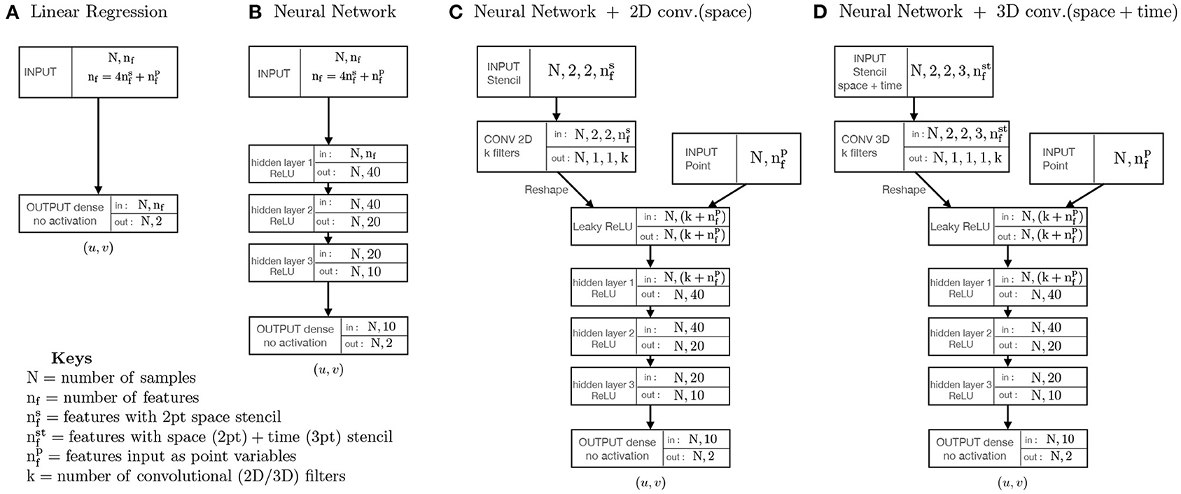
Figure 1. (A–D) Schematic of the four different types of statistical models used in the study. All models shown were implemented using keras tensorflow (Chollet, 2015) and we use Mean absolute error (MAE) as the loss function and the Adam optimizer (Kingma and Ba, 2017) with default parameters and learning rates.

5. Deep Learning: Artificial Neural Networks

Artificial neural networks (or neural networks for short) are machine learning algorithms that are loosely modeled after the neuronal structure of a biological brain but on a much smaller scale. A neural network is composed of layers of connected units or nodes called artificial neurons (LeCun et al., 2015; Nielsen, 2015; Goodfellow et al., 2016) that combine input from the data with a set of weights and passes the sum through the node's activation function along with a bias term, to the subsequent set of nodes, to determine to what extent that signal progresses through the network and how it affects the ultimate outcome. Neural nets are typically “feed-forward,” meaning that data moves through them in only one direction. A layer is called densely connected when each node in that layer is connected to every node in the layers immediately above and below it. Deep learning, or deep neural networks is the name used for “stacked neural networks”—i.e., networks composed of several layers.

Our neural network code was written using the Python library Keras (https://keras.io) (Chollet, 2015), a high-level wrapper around TensorFlow (http://www.tensorflow.org). The feed-forward NNs consist of interconnected layers, each of which have a certain number of nodes. The first layer is the input layer, which in our case is a stacked vector containing the input variables just like in the linear regression example above. The last layer is the output layer, which is a stacked vector of the two outputs (U,V). All layers in between are called hidden layers. The activation function, i.e., the function acting on each node – is a weighted sum of the activations in all nodes of the previous layer plus a bias term, passed through a non-linear activation function. For our study, we used the Rectified Linear Unit (ReLU) as an activation function. The output layer is purely linear without an activation function. Training a NN means optimizing the weight matrices and bias vectors to minimize a loss function—in our case the MAE—between the NN predictions and the true values of (u, v).

The model reduces the loss, by computing the gradient of the loss function with respect to all weights and biases using a backpropagation algorithm, followed by stepping down the gradient—using stochastic gradient descent (SGD). In particular we use a version of SGD called Adam (Kingma and Ba, 2014, 2017). Although most neural network strategies involve normalizing the input variables, we did not use any normalization, since the normalization factors would be largely dependent on the choice of domain/ocean basin, given that the dynamical parameters (like SSH and wind stress) vary widely across the different ocean basins. Instead we wanted the NN to be generalizable across the whole ocean.

We construct a three-hidden-layer neural network to replace the linear regression model described in the previous section. A schematic model architecture for the neural network is presented in Figure 1B. Using the same basic model architecture, we train three NNs on the same three subdomains (Gulf Stream, Kuroshio, ACC) along with one which is trained on the global ocean. Everything including batch size, the training data, the targets, the input features and the number of epochs the model is trained for in each region is kept exactly the same as what we used for the linear regression examples. The only thing that we changed is the model, where instead of one layer with no activation we now have three hidden layers with a total of 1,812 trainable parameters.

5.1. Neural Networks With Convolutional Filters

In section 2 we explained how we can use the local 2 × 2 stencil to expand the feature vector space by a factor of 4. We can further expand the feature vector space by passing all the stenciled input features through k convolutional filters of shape 2 × 2. If $k>4n_f^s$ where $n_f^s$ is the number of input features with a stencil, we end up with more input features that goes into the NN than before. There is very little functional difference between this kind of training approach and the one discussed previously, except that we end up with more trainable parameters, which we can potentially use to extract even more information from the data. We should point out that this is technically not the same as convolutional neural networks (CNN), where the convolutional layers serve to reduce the feature vector space without losing information. This is particularly important for problems like image classification where it is needed to scale down large image datasets without losing feature information. Typically in a CNN, the inputs would be in the form of an image or a set of stacked images on which multiple convolutional filters of varying sizes could be applied (followed by max-pooling layers) that effectively shrink the input size, before passing it on to the hidden layers, and the size of the convolutional filters determine the size of the stencil¹. Whereas in this approach, we use convolutional filters (without max-pooling) to achieve the opposite effect, i.e., to expand the feature vector space from $N\times 2\times 2\times n_f^s$ to N × k (where k is always chosen to be $>4n_f^s$). The reshaping of the input variables in the pre-processing stage fixes the stencil size, before the data is fed into the model.

A schematic of this subcategory of neural network is shown in Figure 1C. After applying the convolutional filter and passing it through a reshape layer in keras the point inputs and filtered stencil inputs are passed through a Leaky ReLU before being fed into a similar three-hidden layer NN framework as described before. Using a similar procedure, we can also apply k 3D convolutional filters of shape 2 × 2 × 3 on the time and space stenciled inputs to effectively end up with k input features of length N for the stencil variables (Figure 1D). The goal with the time stenciled input being to potentially learn time derivatives and explore how the tendencies can affect the NN projections. In hindsight, this data set is probably not be the most suited for this kind of approach since the variables we used as input features are daily averaged and any fast-time scale/tendency effects that we hoped to capture from multiple snapshots of the same variable are probably filtered out by the time averaging. These two approaches are virtually identical with slightly different preprocessing of the input data.

6. Results

We start by splitting the global ocean into three boxes to zoom into three distinct regions of dynamical importance in oceanography, namely the Gulf stream, Kuroshio, and Southern ocean/Antarctic circumpolar current (ACC). The Kuroshio region is chosen to extend south of the equator to include the equatorial jets as well as to test whether the models can generalize to large variations in f. The daily averaged GCM output surface speed on a particular reference date, with the three regions (marked by three different colored boxes) is shown in Figure 2. We then train three different linear regression models with training data from these three sub-domains. We also trained a linear regression model for the whole globe using the same model architecture. During training, the models are fed a shuffled batch of the training data with 32 samples in each batch and the loss (MAE) is computed for the batch. For the linear regression model as well as for all the neural networks discussed in this study we present here we kept the batch size constant. Changing the batch size does not significantly alter the loss at the end of training, but smaller batch sizes generally help the model learn faster. The different models, the number of epochs (an epoch is defined as one pass through the training dataset) used for each, and losses at the end of training and during evaluation against a test dataset are summarized in Table 1. The evolution of model loss function during training for the 3 different models are presented in Figure 3. Linear regression is shown in the darker colors. The big jumps in the loss function correspond to the end of an epoch. We plot the models' training progress in the Gulf Stream region for 8 epochs, and for 5 epochs on the Kuroshio and ACC regions. The trained models are then evaluated for a test dataset (which the model has not seen, GCM output from a different point in time) and the evaluation loss is plotted as the horizontal dashed lines. The linear regression model trained on the whole globe is also evaluated for each subdomain (gulf stream, Kuroshio, ACC) and the global model evaluation loss is plotted as the dotted line. Comparing the model losses in the three different sections, we find that the linear regression model performs the most poorly for the Kuroshio region (i.e., the subdomain with the most variation in f). The model does progressively better for the gulf stream and the ACC in terms of MAE, where the variations in f are relatively smaller in comparison. However, the root mean squared error of predicted velocities is still quite large in all these regions (second panels of Figures 4–6). The linear regression model trained on the global ocean does even worse during evaluation. Since geostrophy relies on non-linear combination of the Coriolis parameter (f) with the spatial gradients, linear regression is ineffective at predicting velocities beyond localized regions with small variation of f or little mesoscale activity. This shows that a linear model fails to accurately represent surface currents in any region that includes significant variation in the Coriolis parameter f. Even in regions far enough from the equator such that the variation in f is not significant (like the gulf stream or ACC), the performance of such a linear model does not improve with more training examples and/or starts overfitting. We also show that a lower MAE during training does not necessarily guarantee that the model is picking up on the small scale fluctuations in velocity, as can be seen from the relatively large squared errors especially in and around high surface current regions (Figures 4–6). We suspect that this failure is largely due to the fact that the linear model is trying to fit the velocities as a linear combination of the different features, whereas realistic surface current predictions should be based on non-linear combinations of features.

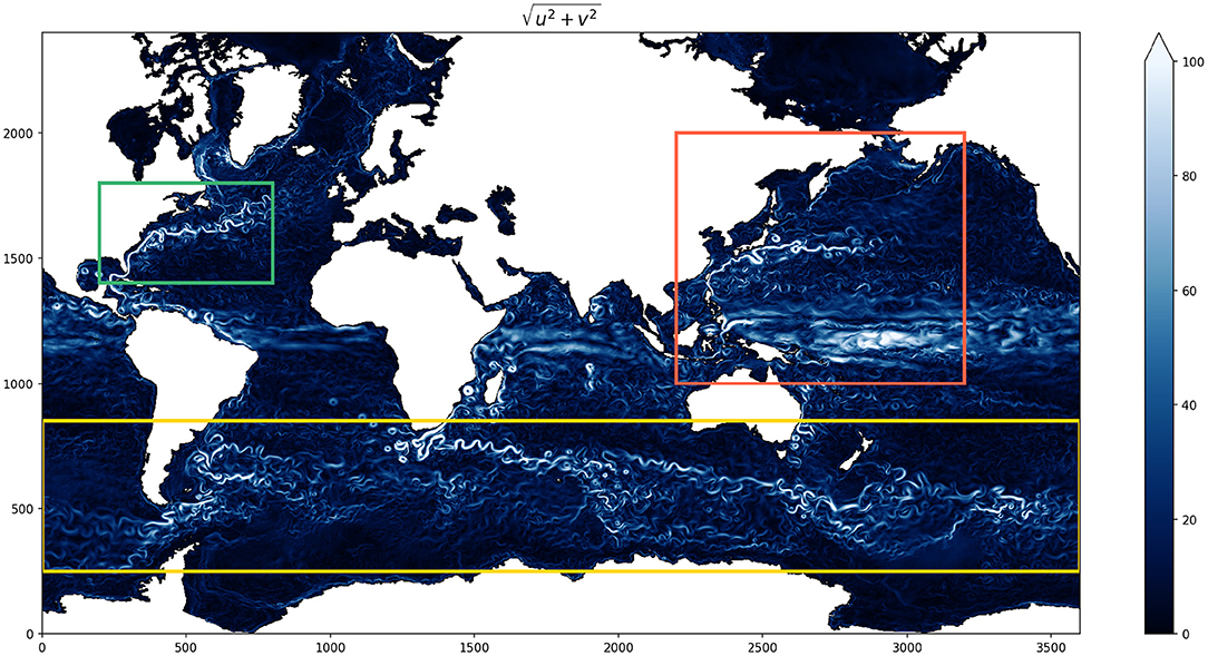
Figure 2. Snapshot of the surface speed in the CESM POP model with the three boxes in different colors indicating the training regions chosen for the different regression models. The green box is chosen as the Gulf stream region, the red box is Kuroshio and the yellow box represents the Southern Ocean/Antarctic circumpolar current (ACC). The Kuroshio region extends slightly south of the equator to include the equatorial jets in the domain and to test the models' ability to generalize to large variations in f.

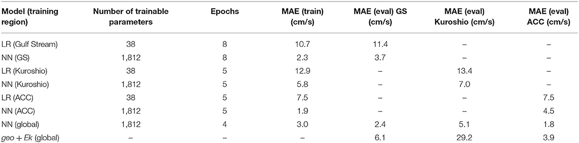
Table 1. Table summarizing model errors from the physics based model (geostrophy + Ekman flow) and the two types of regression models—linear regression and neural network (Figures 1A,B).

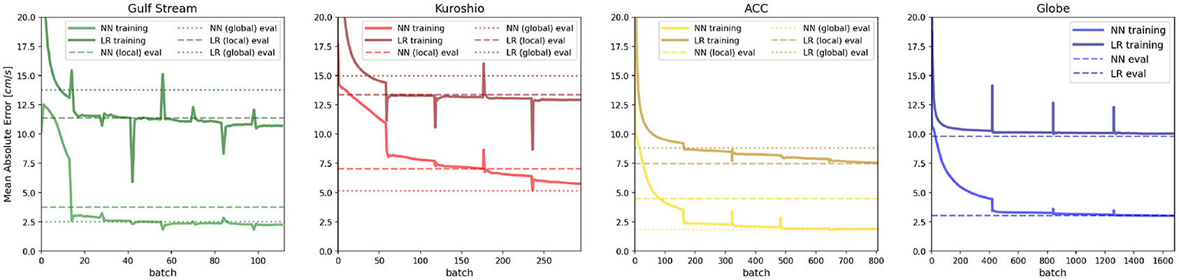
Figure 3. Evolution of the loss function (mean absolute error; MAE) for Neural Networks and Linear regression models during training. Horizontal lines of the corresponding color denote the MAE for the model when evaluated at a different time snapshot. Dashed lines denote the evaluated (test data) MAE for the local model and dotted lines denote that for the model trained on the globe.

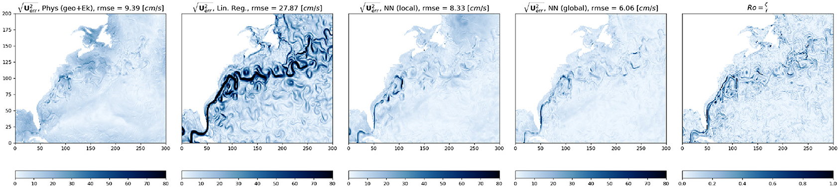
Figure 4. Snapshot of model predicted root square errors for the physics based model (left) and the three different regression models—Linear regression (second from left), neural network, trained on this local domain (third panel) and neural network, trained on the globe (4th panel) compared side by side with the local Rossby Number (Ro, right panel) in the Gulf Stream region indicated by the green box in Figure 2.

Neural networks on the other hand, due to the presence of multiple dense interconnected layers can be effectively used to extract these non-linear relationships in the data. Just like we did with the linear regression model, we tracked the evolution of the loss function as the model scans through batches of input data over multiple epochs (Figure 3, lighter colored lines in all panels). As we can see, in comparison to the linear regression model, the NNs perform significantly better at reducing the loss in all the ocean regions. What is even more striking is that the NN trained on the globe (dashed line) consistently outperforms the local models, predicting surface currents with lower MAE/MSE than the models trained on the local subdomains. This is especially noticeable for the Kuroshio region (Figure 3, second panel), where the NN trained on the globe manages to get the signature of the equatorial currents better than the NN trained specifically in that region (compare panels 3 and 4 of Figure 5) and gets the absolute error down to ≈5 cm/s. This shows, that in comparison to the linear model the neural network actually manages to learn the physics better when it receives a more spatially diverse input data, and is therefore more generalizable. Even though the linear regression models all manage to get the loss down to comparable magnitude, looking at the spatial plot of the predicted squared error. Figures 4–6 gives us an idea how poorly it does at actually learning the physics of surface currents. In comparison, even a relatively shallow three-hidden-layer neural network performs significantly better with very few localized hotspots of large errors. This is to be expected since the largest order balance, i.e., geostrophy relies on non-linear combination of the Coriolis parameter (f) with the spatial gradients.

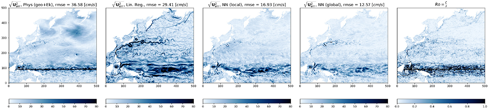
Figure 5. Snapshot of model predicted root square errors for the physics based model (left) and the three different regression models—Linear regression (second from left), neural network, trained on this local domain (third panel) and neural network, trained on the globe (4th panel) compared side by side with the local Rossby Number (Ro, right panel) in the Kuroshio region indicated by the red box in Figure 2. Note the large errors in all the model predictions near the equator.

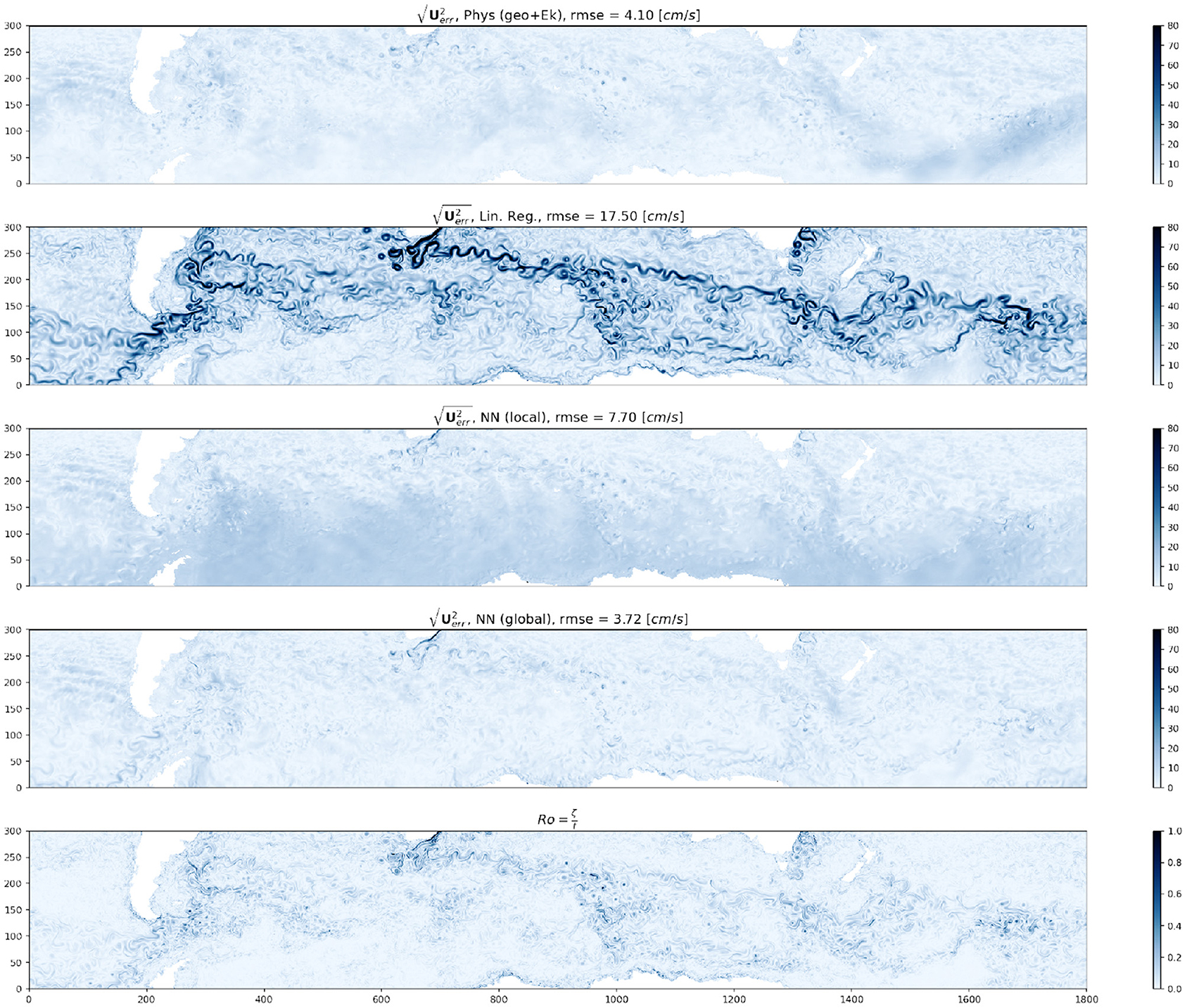
Figure 6. Snapshot of model predicted root square errors for the physics based model (top) and the three different regression models—Linear regression (second panel), neural network, trained on this local domain (third panel) and neural network, trained on the globe (4th panel) compared side by side with the local Rossby Number (Ro, bottom panel) in the Southern Ocean/Antarctic circumpolar current region indicated by the yellow box in Figure 2.

In Figure 7 we plot the joint histogram of the zonal and meridional velocity predictions against the true (GCM output) values for the physical model, linear regression model (trained on the local subdomain) and the locally and globally trained neural networks in the ACC sector. From these joint histograms, it is obvious that the physical model, the local and global neural networks all predict velocities that are extremely well-correlated with the true velocities in this region. In addition the root mean squared (rms) errors normalized by the rms velocities are also very well-correlated between the physical model and neural network predictions. This provides us with reasonable confidence that the model is indeed learning the physics of surface geostrophy and Ekman flow.

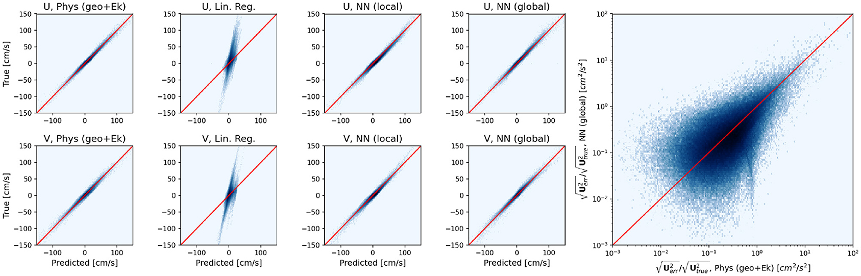
Figure 7. Scatterplot of true v predicted zonal and meridional velocities for the different physical and regression models (eight panels on the left) in the ACC region. The right panel shows the scatterplot of the root mean squared errors (normalized by the root mean square velocities) for the physical and neural network model predictions.

We also plotted the squared errors in predicted velocity form the physical model (geostrophy + Ekman) and the local Rossby number (expressed as the ratio of the relative vorticity ζ = v_x − u_y, to the planetary vorticity f) in the three domains (Gulf Stream—Figure 4; Kuroshio—Figure 5; and the ACC—Figure 6). It is interesting to note that the localized regions in large root squared errors in both the neural network and physical models coincide with regions where the local Rossby number is high. High Rossby numbers indicate unbalanced flow and the specific regions where we see high Rossby numbers are typically associated with heightened submesoscale activity. We speculate that the prediction errors in these locations are due to the NN's inability to capture higher order balances (e.g., gradient wind, cyclostrophic balance) that are necessary to fully capture the small scale variability associated with these motions and close the momentum budget.

The NN also generally predicts weaker velocities near the equator where the true values of the surface currents are quite large (due to strong equatorial jets). This can lead to large errors for the global mean, which get magnified when the differences are squared. However, we know that geostrophic and Ekman balance also doesn't hold near the equator. A fairer comparison would therefore involve masking out the near equatorial region (5°N − 5°S) for both the statistical model (i.e., NN predictions) as well as for the physical model (geo + ekman).

6.1. Model Dependence on Choice of Input Features

We then trained these NNs with varying combinations of input features to explore how the choice of input features can influence the model training rate and loss. Feeding the NN models varying combination of input features, either as stencilled or as point variables and by selectively holding out specific features for each training case allowed us to assess the relative importance of each physical input variable for the neural network's predictive capability. The different models with their corresponding input features and the number of trainable parameters for each case are summarized in Table 2. As with all previous examples, we chose mean absolute error as the loss function for all these experiments. We performed a few training exercises using the mean squared error instead and did not notice any significant difference. For models numbered 1–13, we used a two point space-stencil and for models 1t–10t, in addition to a stencil in space, we provide a three point time stencil with the intention of helping the neural network “learn” time derivatives. The different experiments listed in Table 2, can broadly be categorized into six groups based on their input features. In group 1, is model 1, where the model only sees η (stencil) and wind stress, τ (point) as input features. No spatial information is provided. In the second category, we have models that receive η (stencil) and spatial information X in some form, but no wind stress. This includes models 2, 5t, and 7t. The third category describes models that receive η, θ (stencil) and spatial information X and no wind stress and includes models 3, 6t, and 8t. The fourth category describes models that receive SSH (η), spatial information (X) and wind stress (τ) but no SST and includes models 4, 6, 7, 10, 1t, and 3t. The fifth category of models receive SSH (η), SST (θ), spacial information (X), and wind stress and the only input feature these models don't receive in any form is sea surface salinity (S). This includes models 5, 8, 9, 11, 2t, 4t. The sixth and final category represents models tat receive all the input features (η, θ, S, X, τ) in some form or another and includes models 13, 9t, and 10t.

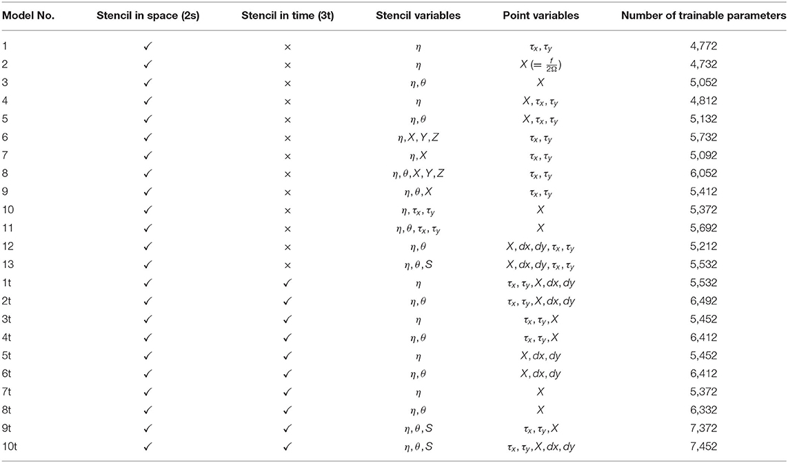
Table 2. Table summarizing the different CNNs and the training strategies explored.

As mentioned previously, spatial information is provided in one of three ways, (a) in the form of three dimensional transformed coordinates (X, Y, Z), (b) just the Coriolis parameter (X here serves as a proxy for the Coriolis parameter) and (c) with both the Coriolis parameter and local dx and dy values. Barring a few examples (models 10, 11) windstress is always provided as a point variable and apart from models 6, 7, 8, 9, none of the models receive a stencil in the spatial coordinates. We also trained a few models without SSH as an input feature, but the loss in all these cases was much larger than those shown here (>50 cm/s) and the NNs fail to pick up any functional dependence on the input features. Those cases are therefore not presented. Each of these models are trained for 4 Epochs on the same day of data (or 3 consecutive days centered around that date for the time stencilled cases).

In Figure 8 we summarize the findings from these experiments by plotting the rms error for all the model predictions along with the rms error for the physical model predictions side by side. With the exception of five models (model 1, 5t, 7t, 6t, and 8t) all our NN model predictions have lower domain mean squared errors than the physics-based models. In terms of features, model without spatial information has the largest error, followed by models without wind stress (The absolute largest error is for the model without SSH, which is too big to be considered here). This signifies that to accurately represent surface currents, apart from SSH, the most important pieces of information required by the neural networks to successfully learn the physics of surface currents are spatial information and wind stress. It is striking to see how much the model struggles without spatial information. This implies that latitude dependence is a critical component for a NN to be able to predict surface currents accurately. It is only expected since the dynamics of surface currents do depend very strongly on latitude and therefore it is impossible to construct a meaningful prediction model based on just snapshots without any knowledge of latitude.

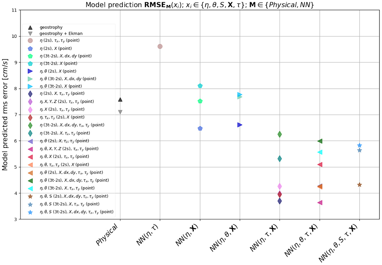
Figure 8. Figure comparing the rms error of the different model predictions along with the rms error for the physical models as a function of features.

The zonal mean rms error for the predictions from some of the representative models from the six categories described above are shown in Figure 9. The NNs all generally predict weaker velocities near the equator where the true values of the surface currents are quite large (due to strong equatorial jets). This can lead to large errors for the global mean, which get magnified when the differences are squared. However, we know that geostrophic and Ekman balance also doesn't hold near the equator. Therefore, to allow for a fair comparison between all the models, we mask out the rms errors in a 10° latitude band surrounding the equator (5°N − 5°S) for both the physical and statistical models. Out of all the models, model 1 which does not receive any spatial information (X), has the highest mean squared errors throughout the globe. For the models that don't see wind stress (τ) as an input feature, the rms errors are comparable if not smaller at most latitudes when compared to the physics-based model where you only consider geostrophy (dashed black line). Additionally, all models that receive η, τ and X in some form perform consistently better than geostrophy + Ekman at all latitudes (except for near the equator where the physics-based models and the NN are all equally inadequate). We noticed that during training, the NN's minimize the loss function slightly faster when a stencil is provided for the spatial coordinates, but after a few epochs the differences in training loss between models that receive a spatial stencil and models that dont, diminish very rapidly. During prediction also, the models that receive stencils in spatial coordinates perform slightly better especially at the high latitudes than the ones where spatial information is provided pointwise.

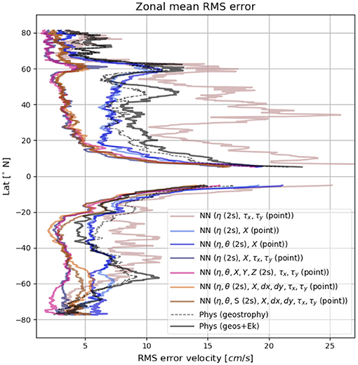
Figure 9. Comparison of the zonal mean rms errors for the various NN predictions shown alongside the physical model (with and without Ekman flow).

Therefore among the various strategies tested, for this particular dataset, the models that perform the best in terms of prediction rms error are the models that receive SSH, wind stress and spatial information with a space stencil. The three point time stencil does not add anything meaningful and appears to hurt, rather than help the model overall, which was surprising, even though in hindsight we speculate that this might be due to the daily averaged nature of the POP model output. Variables like sea surface temperature and sea surface salinity have very little impact on the model as well.

In terms of choice of features, model 13 stands out as the most practical and physically meaningful training strategy for a few reasons.

• It is the most complete in terms of features

• It is the most straightforward to implement, since it does not involve calculating any transformed three dimensional coordinates. (All the input variables would be readily available for any gridded oceanographic dataset.)

• It is one of the models with the lowest prediction rms errors.

For these specific reasons we choose model 13 as the reference for performing a sensitivity analysis. The purpose of this analysis is to characterize the sensitivity of the model to perturbations in the different input features during testing/prediction. For the sensitivity tests we simply add a gaussian noise of varying amplitude to each of the input variables, while keeping the rest of the input variables fixed. For each of the input variables (x_i ∈ {η, θ, X, dx, dy, τ_x, tau_y}), we chose three different zero-mean gaussian noise perturbations with the standard deviations of 0.5σ(x_i), σ(x_i), and 2σ(x_i), where σ(x_i) is the standard deviation of the corresponding input variable x_i. The model loss is then evaluated for each of these perturbations and normalized by the amplitude of perturbations (right panel Figure 10). This normalization is done to level the playing field for all the input variables and allow for a one-to-one comparison since the different input variables vary in orders of magnitude [e.g., the amplitude of perturbations in SSH is O(100), while the amplitude of perturbations in wind stress is O(1) and therefore a perturbation of amplitude σ(η) in η would lead to a much larger model error than a perturbation of σ(τ_x) in τ_x would, as can be seen from the log scaling of the y-axis in the left panel of Figure 10].

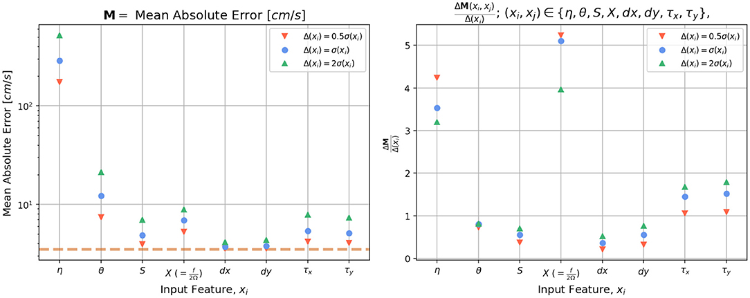
Figure 10. Sensitivity of the neural networks to perturbations in the different input features. Each input feature is perturbed by three different Gaussian noise perturbations with standard deviations of 0.5σ, σ, and 2σ, where σ is the standard deviation of each variable, while keeping the remaining input variables fixed. The left panel shows the model loss (mean absolute error, MAE) evaluated for each of these perturbations. The horizontal dashed line represents the loss for the unperturbed/control case. The right panel shows the deviation in MAE for each of these perturbation experiments normalized by the amplitude of the perturbation.

Given what we learned about the importance of spatial coordinates for NN training, it is not surprising to see that for prediction also, the NN is most sensitive to perturbations in the Coriolis parameter (or X). The input variables that the model is most sensitive to, arranged in descending order of model sensitivity are Coriolis parameter, SSH, and wind stress, followed by SST. The model is not particularly sensitive to perturbations in local grid spacing or salinity. The relative effect of the input variables, observed in the model sensitivity test closely matches what we saw in the different model training examples where we selectively held out these features. This again confirms that in order to train a deep learning model to make physically meaningful and generalizable predictions of surface currents it is not sufficient to simply provide it snapshots of dynamical variables like SSH as images. We also need to provide spatial information like latitude for the NN's to effectively “learn” the physics of surface currents.

7. Summary and Future Directions

The goal of this study was to use machine learning to make predictions of ocean surface currents from satellite observable quantities like SSH wind stress, SST etc. Our central question was: Can we train deep learning based models to learn physical models of estimating surface currents like geostrophy, Ekman flow and perhaps do better than the physical models themselves?

We used the output from the CESM POP model surface fields as our “truth” data for this study. As a first order example, we tested a linear regression model for a few of local subdomains extracted from the global GCM output. Linear regression works well only when the domains are small and far removed from the equator and gets progressively worse as the domain gets bigger and the variation in local Coriolis parameter gets large especially when f changes sign in the domain. This showed that unsurprisingly it is not possible to train a simple linear model to accurately predict surface currents. In addition, providing more data does not necessarily improve the predictive ability of a linear model and only made it worse as it starts overfitting. Whereas, for the same kind of domain, a neural network we can minimize the loss (MAE) with fewer data-points and still remain generalizable, since neural networks can learn functional relationships between regressors (input features) with only a small amount of data. The model's ability to make predictions is also shown to improve with more data. Furthermore, compared to a linear regression model, a NN even with a relatively small network of densely connected nodes, with a suitable non-linear activation function (like ReLU), allows us to have a large number of trainable parameters (weights, biases) that can be optimized to minimize the loss. The activation function is what allows the different non-linear combinations between the different regressors (input features). Somewhat surprisingly, a neural network trained on the entire globe is shown to predict surface currents more accurately in the sub-domains than neural networks trained in those specific sub domains. We suspect that is due to the fact that when trained locally with fewer data points, the neural network only sees part of the distribution of the input variables, as a result of which the stochastic gradient descent settles on a local minima and the model starts overfitting. Whereas, when trained globally, the neural network sees the full distribution of the input variables (not just a section) and SGD settles on a more realistic global minima. This can be observed in Figure 3, in all the local training examples, where model loss at the end of training is consistently lower than the model evaluation loss, when evaluated at a different date. In comparison, a similar approach with a linear regression model produces the opposite result, i.e., a globally trained linear regression model produces higher prediction errors than the one that's trained on each specific sub-domain. However, for linear regression, the evaluation losses are always consistently higher than the training losses, regardless of whether we consider a locally or a globally trained model. The fact that spatially diverse data actually makes the neural network perform better indicates that a neural network can actually “learn” the functional relationships needed for calculating surface currents, i.e., be more generalizable, instead of simply memorizing some target values for different combination of input features. By examining the dependence of the NNs on the choice of input features and by looking at the sensitivity of a NN model to perturbations in the input features, we established that apart from SSH, the physical location of the input features is one of the most crucial elements for the NN to “learn” the physics of surface currents. It is further demonstrated that with a careful and deliberate choice of input features the neural network can even beat the physics-based models at predicting surface currents accurately in most regions of the global ocean. A key ingredient for calculating the Ekman part of the flow using current physics based models is the vertical diffusivity, which is largely unknown for most of the global ocean. Most observational ocean current estimates that include the Ekman part of the flow relies on inferring the vertical diffusivity based on empirical multiple linear regressions with Lagrangian surface drifter data, The neural network approach, by comparison does not suffer from the same kind of limitation, since in this framework, we do not need to provide A_z as an input feature, which is one more added advantage for this method.

In this study, we wanted to see whether we can train a statistical model like a NN with data to essentially match or perhaps beat the baseline physics based models we currently use to estimate surface currents. By examining the errors in surface current predictions from our NN predictions and comparing them with predictions from physically motivated models (like geostrophy and Ekman dynamics), we showed that a relatively simple NN captures most of the large scale flow features equally well if not better than the physical models, with only 1 day of training data for the globe.

However, some key aspects of the flow, associated with mesoscale and sub-mesoscale turbulence are not reproduced. We speculate that this is possibly caused by the fact that the neural network framework can not capture the higher order balances (gradient wind) that are likely at play in these regions since these hotspots of high errors are collocated with regions of High Ro where balance breaks down (see Figures 4–6).

One of the biggest hurdles associated with these studies is figuring out efficient strategies to stream large volumes of earth system model data into a NN framework. So before diving headfirst into the highest resolution global ocean model (currently available), we wanted to test the feasibility of using a regression model based on deep learning as a framework for estimating surface currents with a lower resolution model data (smaller/more manageable dataset), while still being eddy resolving. Hence we chose the CESM POP model data for this present study. In the future, we propose to train a NN with data from a higher spatio-temporal resolution global ocean model like the MITgcm llc4320 model (Menemenlis et al., 2008; Rocha et al., 2016). As a further step, we could coarse-grain such a model to SWOT-like resolutions, or use the SWOT simulator, train NNs on that, and make predictions for global surface currents.

As for the weak surface currents predicted by our NN at the equator, we need to keep in mind that geostrophic balance (defined by the first order derivatives of SSH) only holds away from the equator and satellite altimetry datasets (e.g., AVISO, Ducet et al., 2000) typically employ a higher order balance (Lagerloef et al., 1999) at the equator, to match the flow regime with the geostrophic regime away from the equator. One possible way to train the NN to learn these higher order balances would be by increasing the stencil size around each point. Since our primary goal was for the model to learn geostrophy, we started with a spatial stencil in SSH. We also explored training approaches where we provided stencils in SST, wind and SSS, with the intention of helping the model learn about wind-stress curl and thermal wind balance. In practice, however these didn't payoff as much and these additional stencils did not significantly improve model performance. In future approaches we can try to provide separate stencils of varying size to each of these input variables, to test whether we can further improve the model accuracy.

As another future step, we also aim to incorporate recursive neural networks (RNNs) in conjunction with convolutional filters of varying kernel sizes, to train the models on cyclostrophic or gradient wind balance. This recursive neural network approach would be analogous to iteratively solving the gradient wind equation (Knox and Ohmann, 2006), a technique which was originally developed for numerical weather prediction before advances in computing allowed for integrating the full non-linear equations.

The present work demonstrates that to a large extent, a simple neural network can be trained to extract functional relationships between SSH, wind stress, etc. and surface currents with quite limited data. The field of deep learning as of now is rapidly evolving. It remains to be seen, if with some clever choices of training strategies and by using some of the other more recently developed deep learning techniques, we can improve upon this. In this study, we propose a few approaches that can be implemented to improve upon our current results and would like to investigate this in further detail in future studies. In addition, we believe that data driven approaches, like the one shown in this present study, have strong potential applications for various practical problems in physical oceanography, and require further exploration. Insights gained from this type of analysis could be of great potential significance, especially for future satellite altimetry missions like SWOT.

Data Availability Statement

Publicly available datasets were analyzed in this study. This data can be found at: https://catalog.pangeo.io/browse/master/ocean/CESM_POP/.

Author Contributions

AS and RA: study conception and design and draft manuscript preparation. AS: training and testing of statistical models and analysis and interpretation of results. All authors reviewed the results and approved the final version of the manuscript.

Funding

The authors acknowledge support from NSF Award OCE 1553594 and NASA award NNX16AJ35G (SWOT Science Team).

Conflict of Interest

The authors declare that the research was conducted in the absence of any commercial or financial relationships that could be construed as a potential conflict of interest.

Acknowledgments

The work was started in 2018 and an early proof-of-concept was reported in AS's PhD dissertation (Sinha, 2019).

Footnote

References

Arbic, B. K., Richman, J. G., Shriver, J. F., Timko, P. G., Metzger, E. J., and Wallcraft, A. J. (2012). Global modeling of internal tides: within an eddying ocean general circulation model. Oceanography 25, 20–29. doi: 10.5670/oceanog.2012.38
Bar-Sinai, Y., Hoyer, S., Hickey, J., and Brenner, M. P. (2018). Data-driven discretization: a method for systematic coarse graining of partial differential equations. arXiv.
Bolton, T., and Zanna, L. (2019). Applications of deep learning to ocean data inference and subgrid parameterization. J. Adv. Model. Earth Syst. 11, 376–399. doi: 10.1029/2018MS001472
Bonjean, F., and Lagerloef, G. S. E. (2002). Diagnostic model and analysis of the surface currents in the tropical Pacific Ocean. J. Phys. Oceanogr. 32, 2938–2954. doi: 10.1175/1520-0485(2002)032<2938:DMAAOT>2.0.CO;2
Chapman, C., and Charantonis, A. A. (2017). Reconstruction of subsurface velocities from satellite observations using iterative self-organizing maps. IEEE Geosci. Rem. Sens. Lett. 14, 617–620. doi: 10.1109/LGRS.2017.2665603
Chollet, F. (2015). Keras. Available online at: https://keras.io
Ducet, N., Le Traon, P. Y., and Reverdin, G. (2000). Global high-resolution mapping of ocean circulation from topex/poseidon and ERS-1 and -2. J. Geophys. Res. Oceans 105, 19477–19498. doi: 10.1029/2000JC900063
Gentine, P., Pritchard, M., Rasp, S., Reinaudi, G., and Yacalis, G. (2018). Could machine learning break the convection parameterization deadlock? Geophys. Res. Lett. 45, 5742–5751. doi: 10.1029/2018GL078202
Goodfellow, I., Bengio, Y., Courville, A., and Bengio, Y. (2016). Deep Learning, Vol. 1. Cambridge, MA: MIT Press.
Gregor, L., Kok, S., and Monteiro, P. M. S. (2017). Empirical methods for the estimation of southern ocean CO2: support vector and random forest regression. Biogeosciences 14, 5551–5569. doi: 10.5194/bg-14-5551-2017
Knox, J. A., and Ohmann, P. R. (2006). Iterative solutions of the gradient wind equation. Comput. Geosci. 32, 656–662. doi: 10.1016/j.cageo.2005.09.009
Lagerloef, G. S. E., Mitchum, G. T., Lukas, R. B., and Niiler, P. P. (1999). Tropical pacific near-surface currents estimated from altimeter, wind, and drifter data. J. Geophys. Res. Oceans 104, 23313–23326. doi: 10.1029/1999JC900197
LeCun, Y., Bengio, Y., and Hinton, G. (2015). Deep learning. Nature 521:436. doi: 10.1038/nature14539
Lguensat, R., Sun, M., Fablet, R., Mason, E., Tandeo, P., and Chen, G. (2017). Eddynet: a deep neural network for pixel-wise classification of oceanic eddies. CoRR abs/1711.03954. doi: 10.1109/IGARSS.2018.8518411
Ling, J., Kurzawski, A., and Templeton, J. (2016). Reynolds averaged turbulence modelling using deep neural networks with embedded invariance. J. Fluid Mech. 807, 155–166. doi: 10.1017/jfm.2016.615
Menemenlis, D., Campin, J. M., Heimbach, P., Hill, C., Lee, T., Nguyen, A., et al. (2008). “ECCO2: high resolution global ocean and sea ice data synthesis,” in Mercator Ocean Quarterly Newsletter, 13–21.
Morrow, R., Blurmstein, D., and Dibarboure, G. (2018). “Fine-scale altimetry and the future SWOT mission,” in New Frontiers in Operational Oceanography, eds E. Chassignet, A. Pascual, J. Tintoré, and J. Verron (GODAE OceanView) 191–226. doi: 10.17125/gov2018.ch08
Pathak, J., Hunt, B., Girvan, M., Lu, Z., and Ott, E. (2018). Model-free prediction of large spatiotemporally chaotic systems from data: a reservoir computing approach. Phys. Rev. Lett. 120:024102. doi: 10.1103/PhysRevLett.120.024102
Rocha, C. B., Chereskin, T. K., Gille, S. T., and Menemenlis, D. (2016). Mesoscale to submesoscale wavenumber spectra in drake passage. J. Phys. Oceanogr. 46, 601–620. doi: 10.1175/JPO-D-15-0087.1
Sinha, A. (2019). Temporal variability in ocean mesoscale and submesoscale turbulence (Ph.D. thesis), Columbia University in the City of New York, New York, NY, United States.
Small, R. J., Bacmeister, J., Bailey, D., Baker, A., Bishop, S., Bryan, F., et al. (2014). A new synoptic scale resolving global climate simulation using the community earth system model. J. Adv. Model. Earth Syst. 6, 1065–1094. doi: 10.1002/2014MS000363
Smith, R., Jones, P., Briegleb, B., Bryan, F., Danabasoglu, G., Dennis, J., et al. (2010). The Parallel Ocean Program (POP) Reference Manual Ocean Component of the Community Climate System Model (CCSM) and Community Earth System Model (CESM). Rep. LAUR-01853 141:1–140. Available online at: http://n2t.net/ark:/85065/d70g3j4h
Sudre, J., Maes, C., and Garcon, V. (2013). On the global estimates of geostrophic and ekman surface currents. Limnol. Oceanogr. Fluids Environ. 3, 1–20. doi: 10.1215/21573689-2071927
Sudre, J., and Morrow, R. A. (2008). Global surface currents: a high-resolution product for investigating ocean dynamics. Ocean Dyn. 58:101. doi: 10.1007/s10236-008-0134-9
Traon, P. Y., and Morrow, R. (2001). Ocean Currents and Eddies, Vol. 69, Chapter 3. San Diego, CA: Academic Press.
Uchida, T., Abernathey, R., and Smith, S. (2017). Seasonality of eddy kinetic energy in an eddy permitting global climate model. Ocean Model. 118, 41–58. doi: 10.1016/j.ocemod.2017.08.006
Keywords: deep learning-artificial neural network, surface current balance, geostrophic balance, Ekman flow, regression, predictive modeling
Citation: Sinha A and Abernathey R (2021) Estimating Ocean Surface Currents With Machine Learning. Front. Mar. Sci. 8:672477. doi: 10.3389/fmars.2021.672477
Received: 25 February 2021; Accepted: 03 May 2021;
Published: 09 June 2021.
Edited by:
Zhengguang Zhang, Ocean University of China, ChinaReviewed by:
Lei Zhou, Shanghai Jiao Tong University, ChinaChunyong Ma, Ocean University of China, China
Copyright © 2021 Sinha and Abernathey. This is an open-access article distributed under the terms of the Creative Commons Attribution License (CC BY). The use, distribution or reproduction in other forums is permitted, provided the original author(s) and the copyright owner(s) are credited and that the original publication in this journal is cited, in accordance with accepted academic practice. No use, distribution or reproduction is permitted which does not comply with these terms.
*Correspondence: Anirban Sinha, anirban@caltech.edu