Article

Sea Surface Temperature Variability over the Tropical Indian Ocean during the ENSO and IOD Events in 2016 and 2017

1
College of Underwater Acoustic Engineering, Harbin Engineering University, Harbin 150001, China
2
Acoustic Science Technology Laboratory, Harbin Engineering University, Harbin 150001, China
3
School of Marine Science and Ocean Engineering, University of New Hampshire, Durham, NH 03824, USA
4
Department of Biological Sciences, International Islamic University, Islamabad 44000, Pakistan
*
Author to whom correspondence should be addressed.
Atmosphere 2021, 12(5), 587; https://doi.org/10.3390/atmos12050587
Submission received: 23 March 2021 / Revised: 18 April 2021 / Accepted: 28 April 2021 / Published: 1 May 2021

Abstract

:
2016 and 2017 were marked by strong El Niño and weak La Niña events, respectively, in the tropical East Pacific Ocean. The strong El Niño and weak La Niña events in the Pacific significantly impacted the sea surface temperature (SST) in the tropical Indian Ocean (TIO) and were followed by extreme negative and weak positive Indian Ocean Dipole (IOD) phases in 2016 and 2017, which triggered floods in the Indian subcontinent and drought conditions in East Africa. The IOD is an irregular and periodic oscillation in the Indian Ocean, which has attracted much attention in the last two decades due to its impact on the climate in surrounding landmasses. Much work has been done in the past to investigate global climate change and its impact on the evolution of IOD. The dynamic behind it, however, is still not well understood. The present study, using various satellite datasets, examined and analyzed the dynamics behind these events and their impacts on SST variability in the TIO. For this study, the monthly mean SST data was provided by NOAA Optimum Interpolation Sea Surface Temperature (OISST). SST anomalies were measured on the basis of 30-year mean daily climatology (1981–2010). It was determined that the eastern and western poles of the TIO play quite different roles during the sequence of negative and positive IOD phases. The analysis of air-sea interactions and the relationship between wind and SST suggested that SST is primarily controlled by wind force in the West pole. On the other hand, the high SST that occurred during the negative IOD phase induced local convection and westerly wind anomalies via the Bjerknes feedback mechanism. The strong convection, which was confined to the (warm) eastern equatorial Indian Ocean was accompanied by east–west SST anomalies that drove a series of downwelling Kelvin waves that deepened the thermocline in the east. Another notable feature of this study was its observation of weak upwelling along the Omani–Arabian coast, which warmed the SST by 1 °C in the summer of 2017 (as compared to 2016). This warming led to increased precipitation in the Bay of Bengal (BoB) region during the summer of 2017. The results of the present work will be important for the study of monsoons and may be useful in predicting both droughts and floods in landmasses in the vicinity of the Indian Ocean, especially in the Indian subcontinent and East African regions.

1. Introduction

Sea surface temperature (SST) is one of the most critical oceanic parameters. It plays a major role in the development of atmospheric events in the Indian Ocean both on regional and global scales [1,2,3]. The evolution of SST anomalies in the Indian Ocean mainly involves coupled ocean-atmosphere processes [4,5] that are either (i) generated by the large-scale atmospheric forces linked with El Niño/La Niña-Southern Oscillation (ENSO) in the tropical eastern Pacific [6,7,8] or (ii) brought about by an internal independent ocean mechanism such as the Indian Ocean Dipole (IOD) [4,9,10,11,12,13], either of which can affect the interannual variability of SST. The Indian Ocean is considered the warmest ocean in the world in April–May (the Indian Ocean warm pool [14]) and is a major cause of monsoon rainfall [15]. However, the size of the warm pool (which maximizes in April–May) has been reduced by the Somalia–Oman upwelling and also in part by increased latent heat in the Arabian Sea (AS) [16,17]. These warm/cold SST anomalies occur in the western AS due to weak/strong upwellings, respectively, and are the main cause of increased/decreased precipitation anomalies for Indian summer monsoon rainfall [18]. In fact, these SST anomalies, driven by various ocean dynamics (e.g., horizontal and vertical advection, surface-based energy flows, horizontal and vertical wind turbulence), are mainly responsible for causing extreme weather conditions in the Indian Ocean during the monsoon season. They also influence weather and climate over adjoining land areas [19,20]. These extreme weather events in the Indian Ocean may lead to drought situations if break conditions continue for a few weeks. The longevity of active conditions can lead to heavy rain and severe floods [21,22]. These increased drought conditions have a robust relationship with SST variations—particularly in tropical regions—and related variations in atmospheric circulation and rainfall [23]. The dynamics of such variations in monsoon rainfall and other extreme weather conditions are not well understood. However, it is well recognized that the atmosphere interacts with the upper ocean (rather than the surface alone), suggesting that forecasts of the monsoon in the Indian Ocean can be improved by considering upper ocean parameters [24].
Recent studies have focused on the Pacific Ocean as a prospective player in modulating global warming trends due to its huge volume [25,26,27]. The ENSO is an irregularly periodic variation in SST and wind over the tropical eastern Pacific Ocean, with major global socioeconomic and environmental impacts [28]. As can be seen from Figure 1, 2016 was marked by strong El Niño conditions in which maximum positive SST anomalies were confined to the Niño 3.4 region. 2017, in turn, was marked by weak La Niña conditions in which maximum negative SST anomalies were confined to the same region. The 2016 El Niño was one of the first powerful El Niño events of the 21st century and one of the three strongest documented since 1950—together with those of 1997/98 and 1982/83 [29]. Warm conditions persisted, especially from October 2015 to April 2016, when the El Niño impact on global climate was at its peak. Positive equatorial SST anomalies continued across most of the Pacific and Indian oceans, while negative SST anomalies prevailed most of the year in 2017 (Figure 1a,b). The large positive SST anomalies in the eastern Pacific reached a historical high during late 2015 and early 2016. The powerful El Niño in 2016 and weak La Niña in 2017 in the Pacific significantly influenced SST in the Indian Ocean; they were followed by strong negative and weak positive IOD events in 2016 and 2017, respectively. Previous research demonstrated the significant climatic effects of IOD, including the severe East Africa floods that occurred during two extreme positive IOD events in 1994 [30] and 1997 [12,31].
In this study, two contrasting years (2016 and 2017) were chosen to investigate the impact of ENSO and IOD on SST variability in the tropical Indian Ocean (TIO) using various satellite datasets. The dynamics of these two years were unusual and were not thoroughly explored. In that two-year period, a strong El Niño was followed by an extreme negative IOD (in 2016), and a weak La Niña was followed by a positive IOD (in 2017). El Niño in the Pacific Ocean usually favors positive IOD in the Indian Ocean, while La Niña favors negative IOD. These extreme events had a significant impact on Indian Ocean SST variability; they caused significant flooding and above-average rainfall in many parts of Australia, Indonesia, and Bangladesh, and drought conditions in East Africa [29,32]. On the other hand, the positive IOD, in combination with a weak La Niña in 2017, was associated with major climate events, including dry summer conditions in much of Australia, above average rains in the Horn of Africa late in the year after an extended period of drought, and monsoon floods in the Indian subcontinent [33,34]. Another interesting feature of this study was its examination of the cooling/warming in the SST cycle during the summers of 2016/2017. The impact of this was analyzed using data on monsoon rainfall distribution in the Bay of Bengal (BoB) region. The results of these analyses will improve our understanding of the climate system, as we examined it from a better perspective. SST climatology is an essential prerequisite for the ocean modeling community. It may also be useful to study the climate dynamics affecting droughts, floods, severe rainfall events, etc. experienced by landmasses, particularly in the Indian subcontinent and East Africa. This, in turn, would ultimately serve those parts of society whose livelihoods rely on agriculture.
The rest of the paper is structured as follows: Section 2 describes details and analyses of various satellite datasets and measurement of ENSO and IOD indices. The evolution of the IOD in the Indian Ocean in 2016 and 2017 is presented in Section 3.1. Section 3.2 discusses the analysis of SST variability and related mechanisms in the equatorial Indian Ocean and the Arabian Sea region. Section 3.3 provides the precipitation variability and SSS circulation in 2016 and 2017. Section 4 summarizes the main findings.

2. Materials and Methods
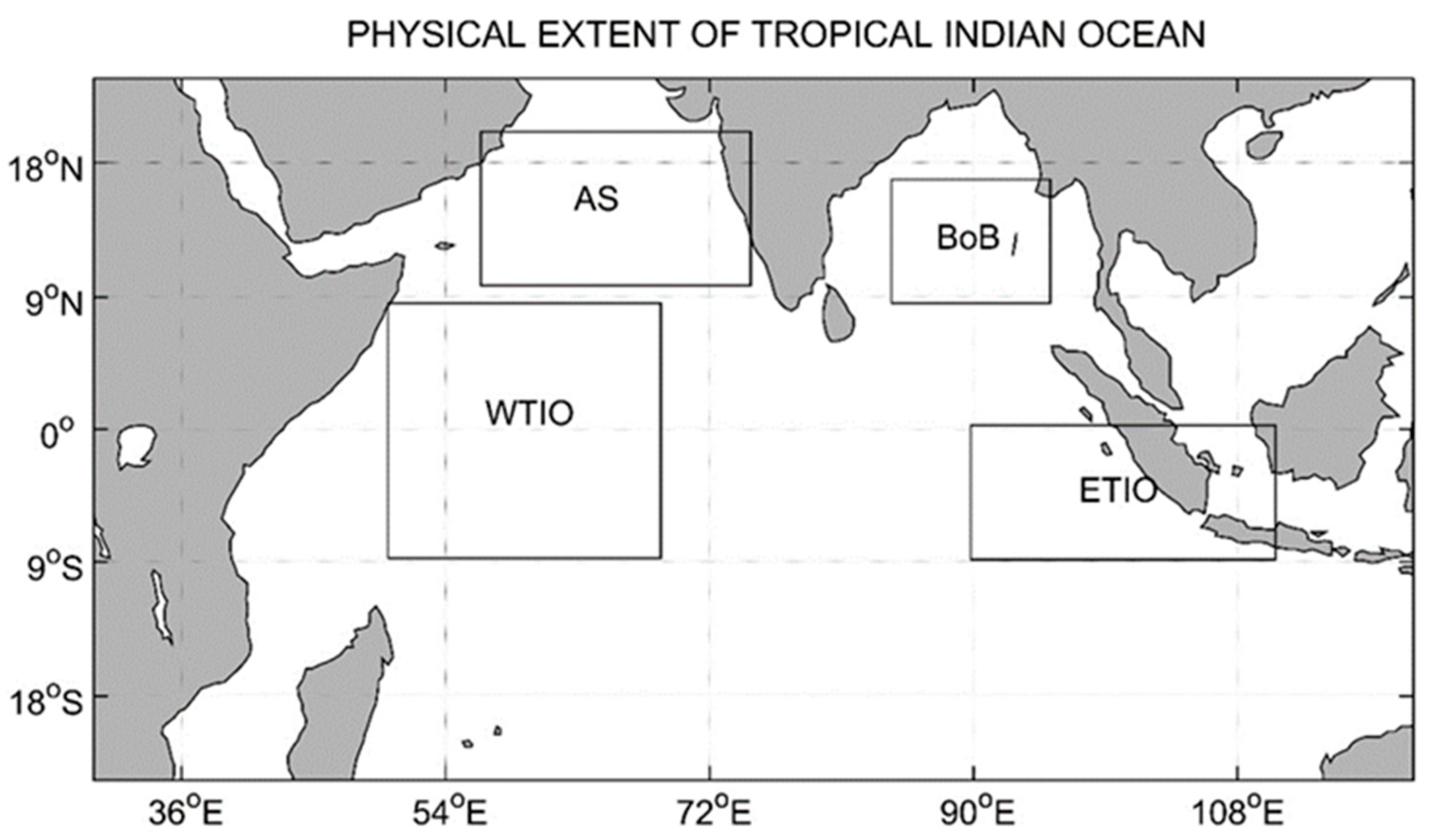
2.1. Study Area

The area under investigation was situated in the TIO. The physical extent of the TIO is shown in Figure 2. As shown in the figure, the black boxes indicate the areas under investigation: eastern tropical Indian Ocean (ETIO), western tropical Indian Ocean (WTIO), and the Arabian Sea (AS). The AS is the northwest part of the TIO, with land boundaries in the west, north and east. It is surrounded by India to the east, Pakistan and Iran to the north, and the Arabian Peninsula to the west. The Gulf of Oman is situated in the northwest corner of the AS. The sea connects with the Persian Gulf via the Gulf of Oman and the Strait of Hormuz. The Gulf of Aden links it with the Red Sea in the southwest. The BoB is the Indian Ocean’s northeastern extension, surrounded on the west and northwest by India, on the north by Bangladesh, and on the east by Myanmar and the Andaman and Nicobar Islands of India.

2.2. Data Source and Analysis

The dynamics of SST variability in the Indian Ocean are different for different seasons and regions. Therefore, monthly mean of SST data for 2016 and 2017 were analyzed separately for each region in this paper. The monthly average SST and SST anomalies data in the selected regions were derived from NOAA OISST (Optimum Interpolation Sea Surface Temperature) blended product, Version 2.1. This product included satellite observations as well as advanced very high-resolution radiometer (AVHRR) and advanced microwave scanning data, and was available from 1981 on, with a 0.25° × 0.25° spatial resolution and daily temporal interval [35,36,37]. The anomalies of SST were measured on the basis of the daily mean climatology of 30 years (1981–2010). The analyses of the data were performed in MATLAB R2017a. Before analysis, the data were interpolated to eliminate missing data from the NOAA daily SST dataset.
The monthly mean sea air temperature (SAT) data were provided by NCEP Global Data Assimilation System (GDAS), available at 2.5° × 2.5° horizontal resolution. The temporal coverage of SAT included daily mean values from 1979 to the present with varying pressure up to 12 levels from 1000 to 50 mb (millibars). In this study, the monthly mean SAT data were computed in the selected regions at 1000 mb pressure level, or about 1 atmospheric pressure. In the tropical oceans, the propagation of the fluctuations in the thermocline is a crucial factor in maintaining the cycles of ENSO and IOD. The changes in the thermocline depths can be represented by the changes in the depths of an isotherm layer. In this study, the depth data of the isotherm layer were provided by Global Ocean Data Assimilation System (GODAS; [38]). GODAS depends on continuous real-time data from the Global Ocean Observing System. For ILD, the criteria used was the depth range where the temperature of given depth (z) is within 0.8 °C of the surface temperature-i.e., ILD=depth where T(z) ≥ SST-∆T, and ∆T = 0.8 °C [39].
In addition, in this study, the precipitation data and wind speed at 10 m above sea surface (U10) were used. The monthly mean precipitation data (mm d−1) were derived from the Global Precipitation Climatology Project Version 2.3 (GPCPv2.3) for reanalysis. The GPCPv2.3 data were available with 2.5° × 2.5° horizontal resolution [40,41]. The long-term dataset of precipitation anomalies (1948–2019) were collected from NOAA precipitation reconstruction (PREC). The climatology of precipitation anomalies was based on time period of 1979–1998 over oceans. The Woods Hole Oceanographic Institution (WHOI) Objectively Analyzed Air Sea Fluxes (OAFlux) project provided the mean wind speed at 10 m above sea surface datasets. The OAFlux is an ongoing research and development project for global air-sea fluxes (http://oaflux.whoi.edu, accessed on 13 July 2020). The daily and monthly means of wind speed data were available at 0.25° × 0.25° horizontal resolution from July 1987 onward. The monthly mean wind speed data were computed in the selected regions for 2016–2017 and missing data were removed for better quality. The monthly mean Sea Surface Salinity (SSS) data were obtained from the SMAPv3 (Soil Moisture Active Passive version 3; [42]), and are accessible online at (www.remss.com/missions/smap, accessed on 18 Septemer 2020). Although SMAP was designed to measure space soil moisture, its L-band radiometer can also be used to measure SSS.

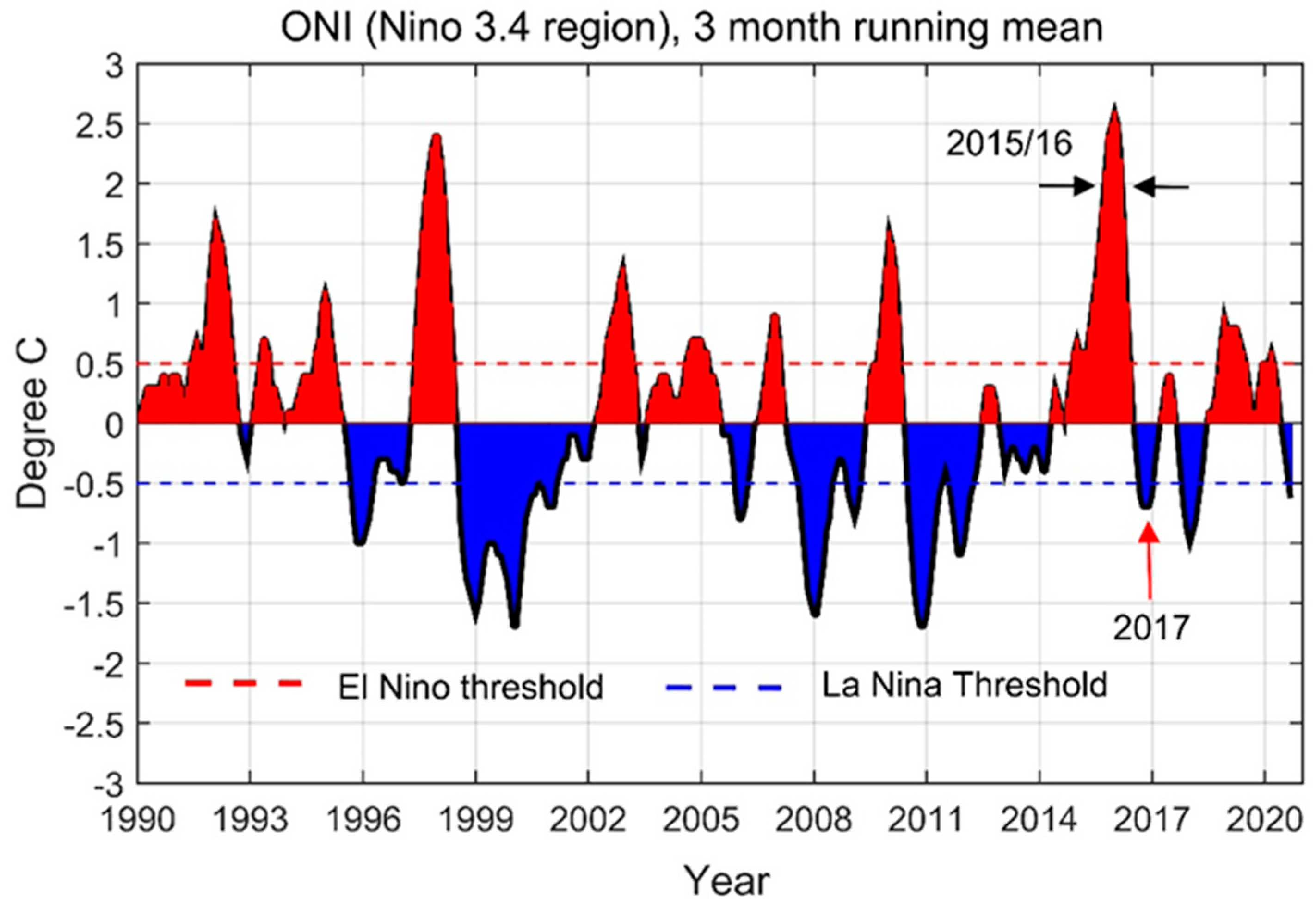
2.3. Measurement of Oceanic Niño Index

The oceanic Niño index (ONI) is a key oceanic variable that describes the El Niño/La Niña phases in the Pacific Ocean. The two phases last several months each, typically occurring with varying intensity per period every few years. El Niño and La Niña are phenomena in the tropical Pacific Ocean described as five consecutive three-month running means of SST anomalies in the Niño 3.4 area (5° S–5° N, 170–120° W) that is above or below the threshold of +0.5 °C or −0.5 °C, respectively. This standard of measure is known as the ONI. The selection criteria of the El Niño/La Niña events were consistent with NOAA Oceanic Niño Index, in which the most recent three-month average SST anomalies in the Niño 3.4 area are considered. If the area is more than 0.5 °C above or below average for that period, El Niño or La Niña conditions are considered to be in progress. Here, we used data from NOAA Extended Reconstructed Sea Surface Temperature version 5 (ERSSTv5; [43]) to measure the strength of ONI from 1990 to 2020, as presented in Figure 3. The data are automatically updated each month and are freely available online at NOAA’s website. The ONI values indicated that strong El Niño conditions developed during November 2014 and persisted for 19 months before decaying in May 2016. The high value of ONI (>2.5 °C), which was observed from November 2015 to February 2016, represents one of the most powerful El Niños since 1990 (Figure 3).

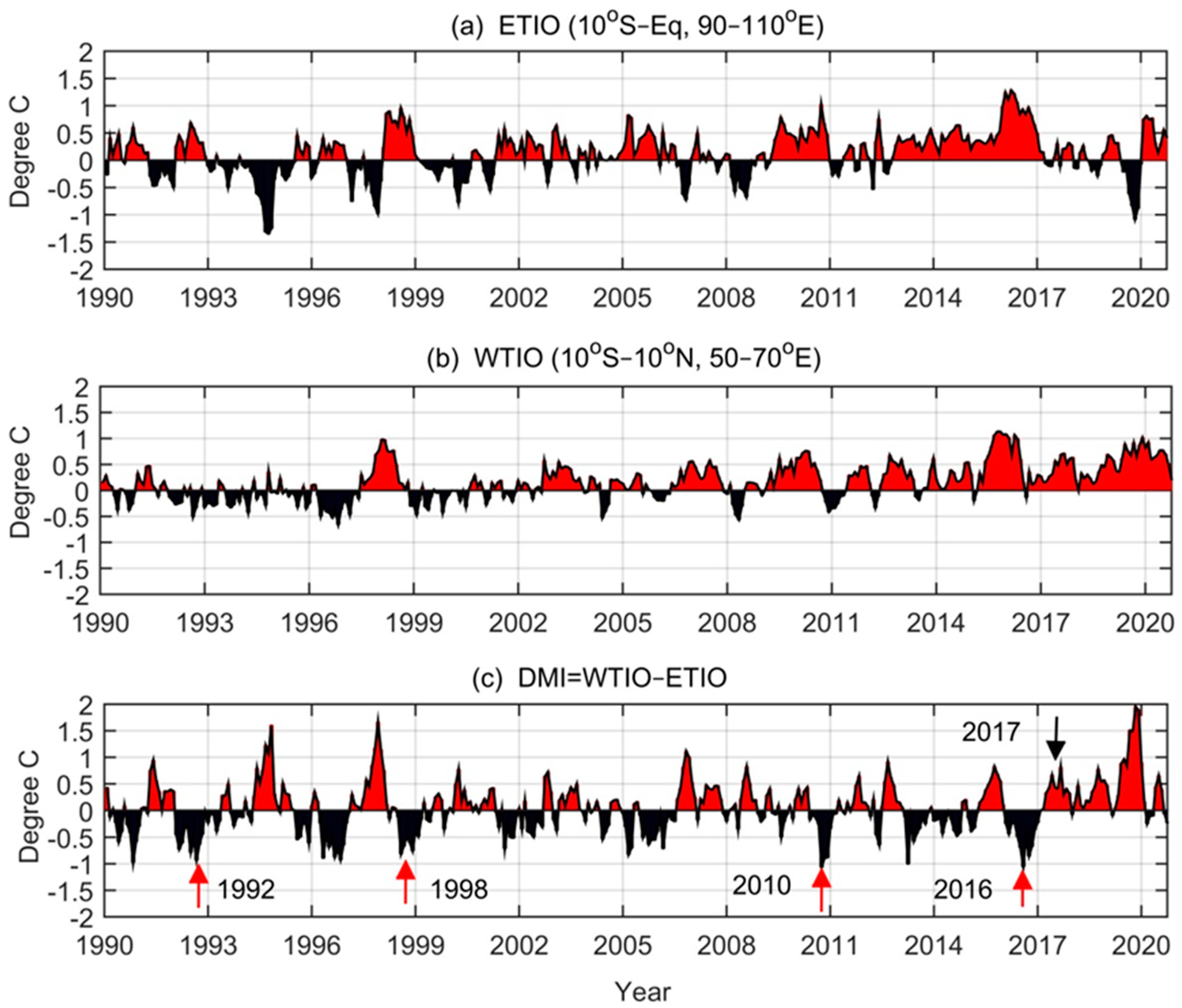
2.4. Measurement of Dipole Mode Index

The dipole mode index (DMI) is a key oceanic parameter that describes the strength of positive/negative IOD phases in the Indian Ocean. As shown in Figure 4a,b, average SST anomalies were estimated for boxes in the ETIO—bounded by (10° S–Eq, 90–110° E)—and WTIO—bounded by (10° S–10° N, 50–70° E)—respectively [11]. In an IOD year, the DMI is expected to be higher than one standard deviation and should remain so for 3 to 4 months. The west-east SST anomalies are positive during a positive IOD year and vice versa. The DMI has been widely used in IOD studies examining its mechanism [11,44,45], predictability [46,47,48,49,50], and effect on climate [51,52]. Here, the DMI was obtained with the averaged SST anomaly of ERSST.V5 datasets [43], from 1990 to 2020, with solid red and blue bars for positive and negative IOD, respectively (Figure 4c). DMI indicated that a strong negative IOD event appeared between June and October 2016, with abnormally warm SST in the ETIO and relatively cool conditions in the WTIO. According to the NOAA OISSTv2 datasets [53], it was the strongest negative IOD event since 1980.

3. Results and Discussion

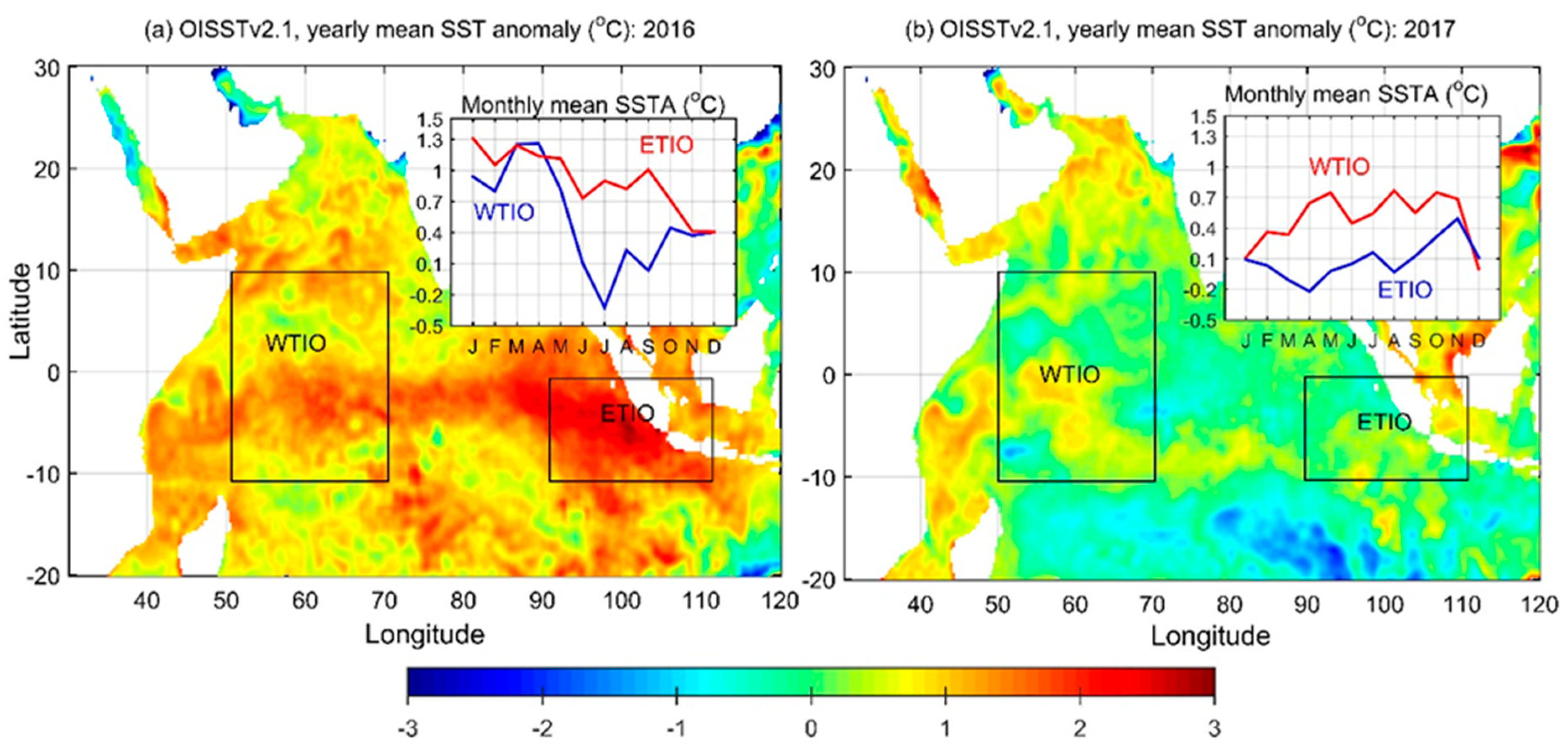
3.1. Evolution of Dipole Structure in 2016 and 2017

Figure 5a shows the development of the strong IOD in 2016, with the western equatorial Indian Ocean being unusually cold and the eastern Indian Ocean being unusually warm [11]. The two black boxes are the WTIO and ETIO in the equatorial Indian Ocean. Following the El Niño event in the Pacific, the Indian Ocean experienced frequent warming as a result of suppressed atmospheric convection and enhanced surface energy flux [54]. This basin-wide warming was noted from January–April 2016, in which the positive SST anomalies persisted in both poles of the equatorial Indian Ocean. The SST anomalies over the western Indian Ocean fell to 0.5 °C below average after the quick demise of the powerful 2015/16 El Niño in April 2016 (Figure 5a).
However, the SST anomalies at the ETIO remained warmer than average during 2016, which is consistent with the persistent negative IOD warming in 1992, 1998, and 2010, following the El Niño events of 1991/1992, 1997/1998, and 2009/2010, respectively (Figure 3 and Figure 5a). The ETIO warmed up again during the summer of 2016, hitting 1 °C above average in September 2016, establishing the most extreme negative IOD event since 1980 [32]—and in the last 63 years during June to September [55]. The DMI exceeded −1 °C, a historical low, in July 2016 (Figure 4c). The temporal variation of SST anomalies showed that the 2016 dipole began during early summer in June and decayed in November. In contrast, a weak positive IOD episode existed for most of 2017, with SST anomalies marginally below the 1981–2010 average over the ETIO and above the WTIO (Figure 5b). Cold SST anomalies suppressed atmospheric convection in the east pole whereas warm SST anomalies enhanced convection in the west pole. This anomalous state of the ocean-atmosphere system is referred to as a positive IOD [11]. The unusual warming and cooling in SST, which occurred in 2016 and 2017, had a strong influence on the climate in the surrounding sea and land areas [29,33].

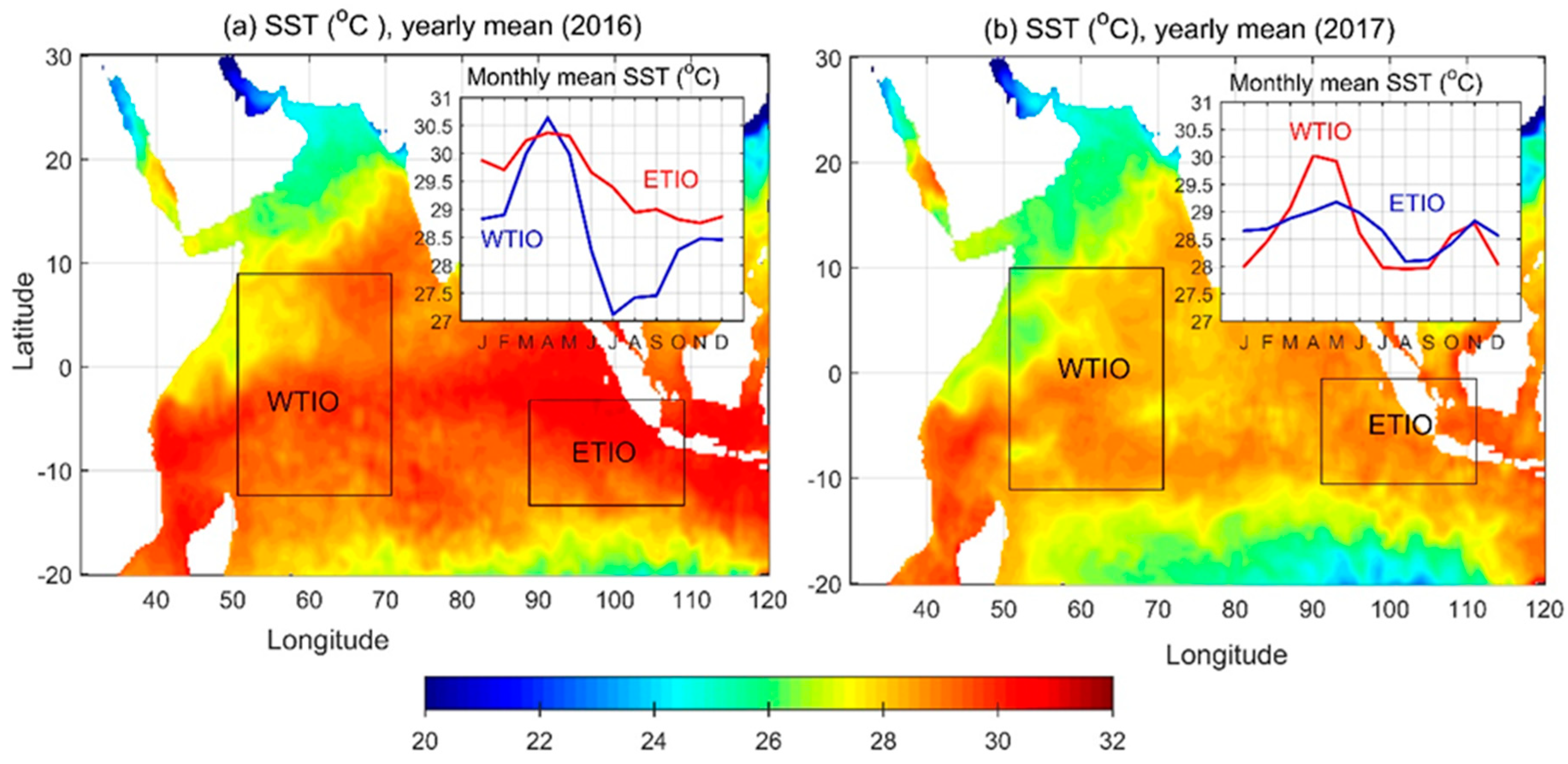
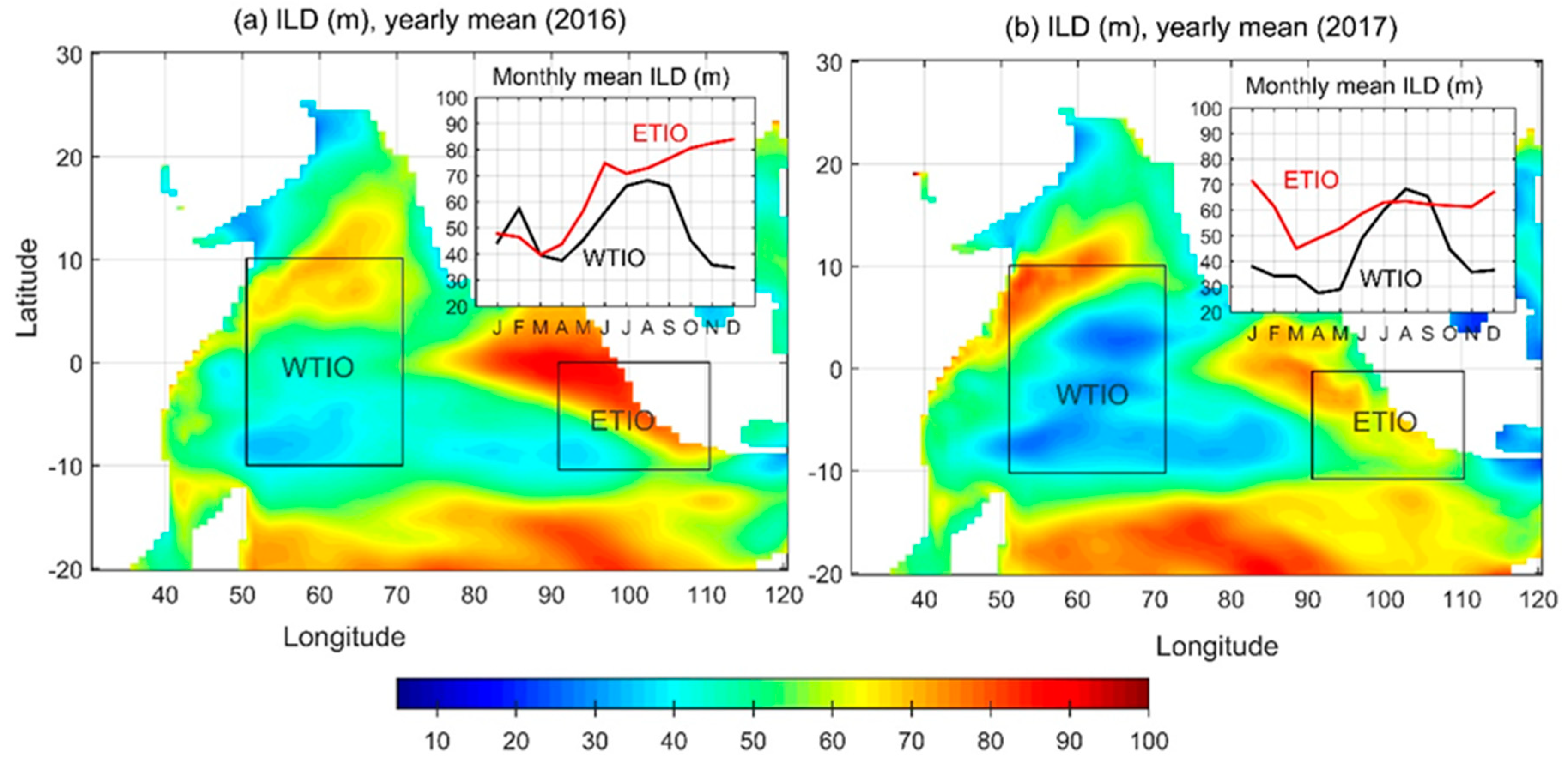
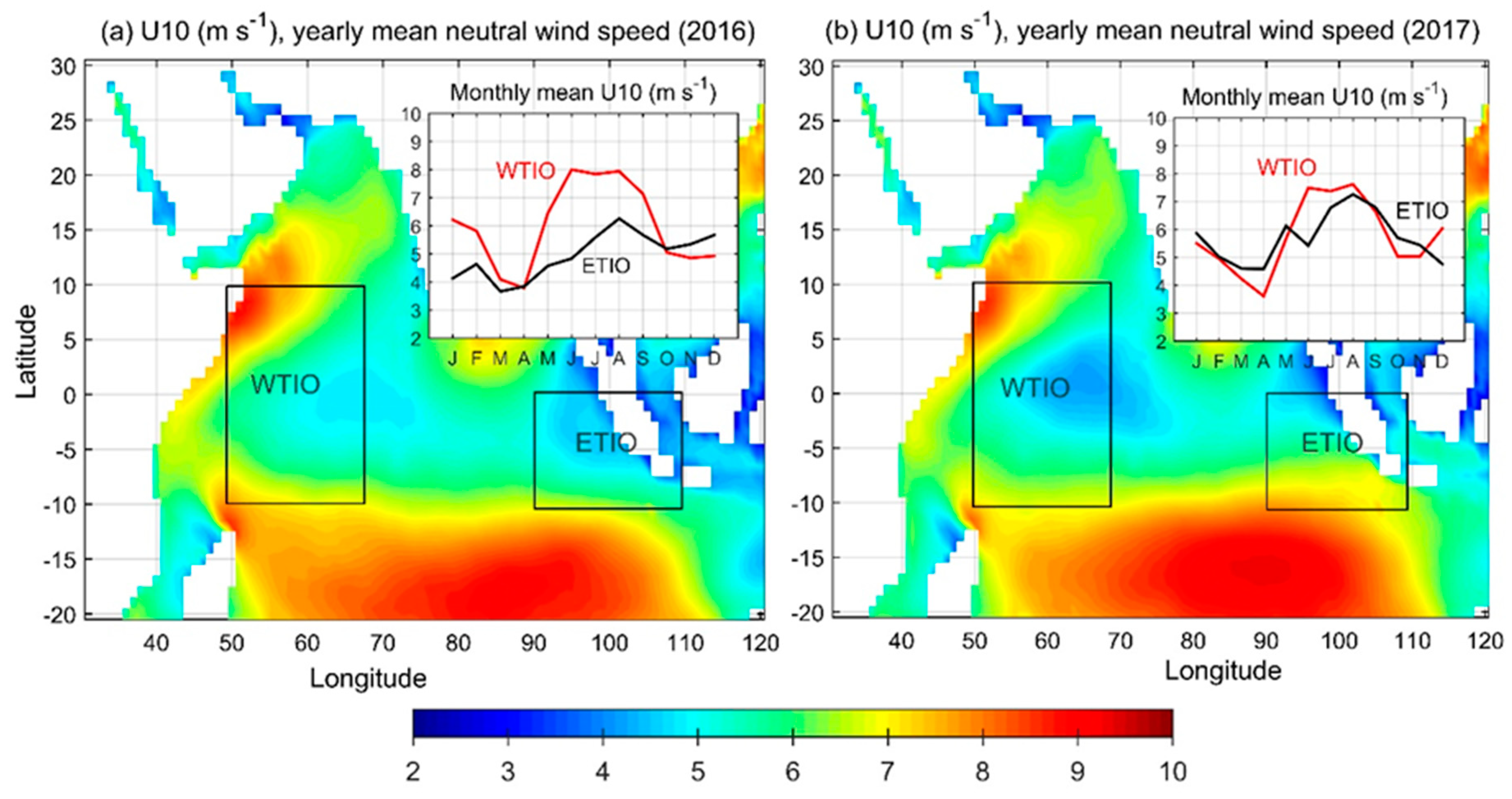
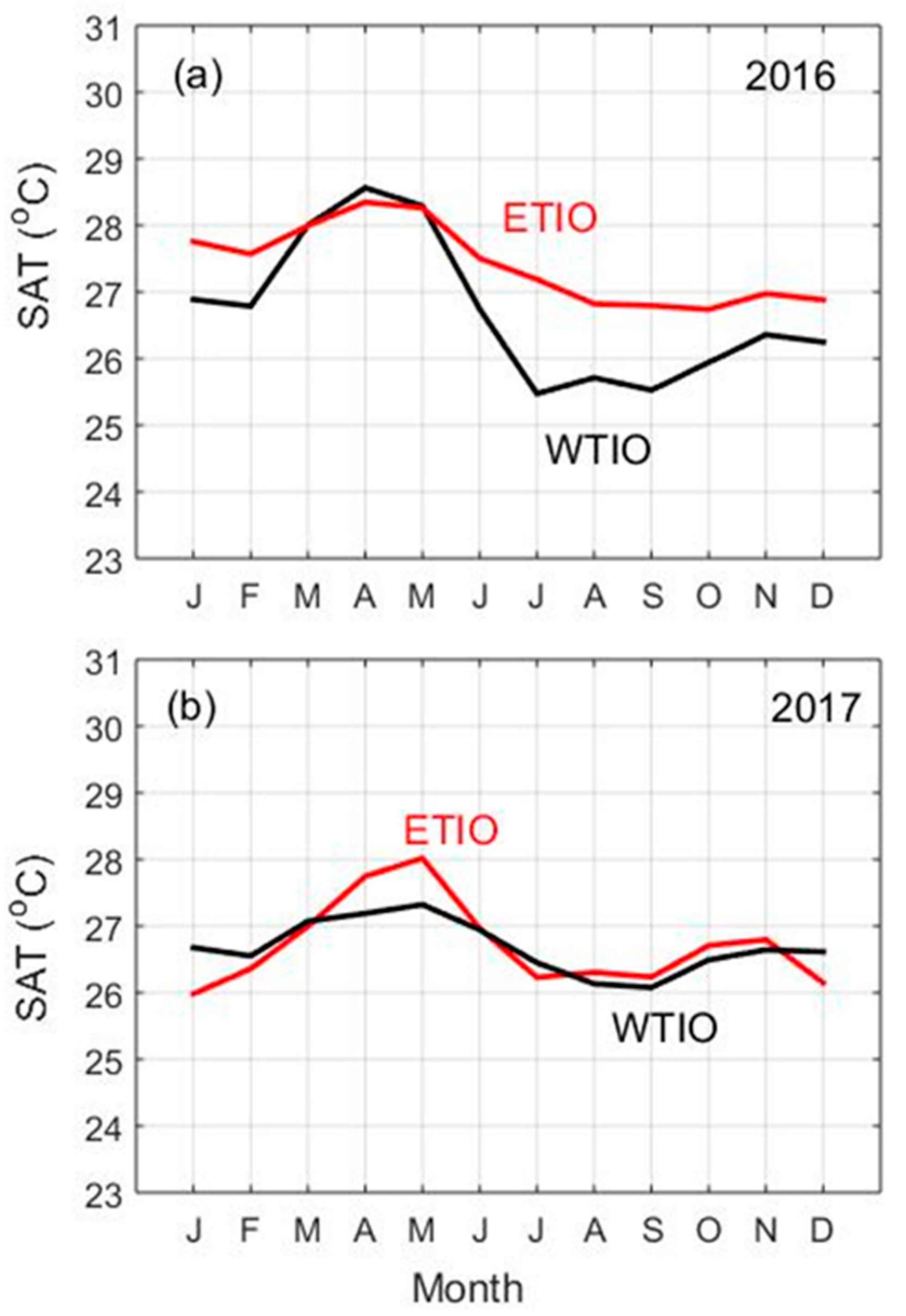
3.2. SST Variability and Associated Mechanisms in the TIO

3.2.1. The Equatorial Indian Ocean Region

SST variability in the TIO during 2016–2017 is shown in Figure 6. As shown in the figure, the seasonal cycle of SST in the western and eastern poles was not consistent, which usually indicates variability. In the WTIO, the SST cooled in the summer and predominantly warmed in the pre-monsoon months. The pre-monsoon warming was most likely due to clear skies, reduced winds, and an increase in solar insolation (absorbed in the upper layer), which induced thermal stratification and suppressed turbulent mixing. This was analogous to the suppression of turbulent kinetic energy [56], which caused the thermocline depth to rise with a shallow isothermal layer depth (ILD), which was reduced (~30 to 40 m) in April–May (see Figure 7). On examining seasonal averages, the pre-monsoon warming periods were dissimilar and varied in both 2016 and 2017. Significant variations in the SST cycle were observed during the pre-monsoon; SST was 1 °C warmer in 2016 than in 2017. The SST reached about 31 °C in April 2016 (versus about 30 °C in 2017). SST warming in 2016 was consistent with the extreme El Niño that began in October 2015 and decayed in May 2016. The powerful El Niño significantly influenced the equatorial Pacific and Indian oceans in which positive SST anomalies persisted until May 2016. The surface wind at 10 m above sea surface (U10) and SAT at 1 atmospheric pressure were around 4 m s−1 and 28.5 °C, respectively (see Figure 8a for surface winds and Figure 9a for SAT). However, the wind speed showed an increasing trend as the monsoon set in. SST grew cool and hit 27 °C in summer 2016 (versus 28 °C in 2017) from July to September, due to strong surface winds (wind > 8 m s−1) and cooling in the air temperature (<26 °C). During this period, the effect of wind force was high (as compared to the pre-monsoon period), and the turbulent mixing caused the cool surface waters to sink into a deeper layer, resulting in a deeper thermocline (up to 70 m). In comparison, the temperature of the sea surface in this region was nearly 1 °C warmer in 2017 than in 2016, which was consistent with our analysis of positive and negative IOD events in 2017 and 2016 with corresponding high and low SSTs in the west pole. The associated anomalously westerly surface wind stress caused upwelling in the WTIO. This upwelling pulled cool subsurface waters upward, increasing the zonal SST gradient between west and east, and reinforcing the negative IOD pattern. Significant correlation was observed between the SST and the wind, representing a strong coupling between the ocean and the atmosphere in the west pole. These variability patterns highlight the fundamental role of wind on the SST in the western basin. In conclusion, the mechanisms describing the air-sea feedback (as well as the relationship between wind and thermodynamic parameters) showed that SST is mainly driven by wind force in this region.
Like the western pole, the eastern pole also experiences SST cooling in the monsoon season and warming in the pre-monsoon season. As can be seen in Figure 6a,b, the SST peaked in April in both years and crossed 30.5 °C in 2016 (versus 29 °C in 2017). But the eastern pole played a rather different role during the sequence of negative and positive IOD events. A slight decrease in the SST was noted in this region during the monsoon period in which the SST reached 29 °C in 2016 (and 28 °C in 2017) in July–September. The SAT in this region remained high in 2016 over the entire period, as opposed to 2017, in which SAT was more pronounced during the first half of the year. It is interesting to highlight that SAT was similar in both poles (except during the pre-monsoon period) throughout 2017. However, the SAT over the eastern basin was warmer than in the west by more than 1.5 °C in the summer of 2016 (Figure 9a,b). This warming in the air temperature was consistent with the strong El Niño which occurred in the eastern Pacific in early 2016. That El Niño impacted the eastern equatorial Indian Ocean region and triggered an unusual strong negative IOD in the Indian Ocean in the summer of 2016.
The strong negative IOD event led to unusual warming in the eastern pole during the summer of 2016. The SST was higher (by 2 °C) than in the western pole, which marked the east-west asymmetry in the Indian Ocean. A close relation between SST and SAT was noted for both 2016 and 2017 and in both poles. However, SAT cooled by around 2 °C more than SST and was more pronounced during the pre-monsoon season (April–May). During the negative IOD event that occurred in the summer of 2016, anomalously high SSTs appeared off the Sumatran coast, inducing local convection and western wind anomalies through the Bjerknes feedback [57]. The surface wind patterns were similar in the east and west poles in 2017; however, weak surface wind (wind < 6 m s−1) in the eastern basin and strong surface wind in the western basin (wind > 8 m s−1) appeared more pronounced from May to September 2016 (Figure 8a,b). This anomalous increase in wind speed reduced SST (up to 2 °C) in the western basin in 2016. This basin-wide variability in SST that appeared in summer 2016 highlighted the fundamental role of wind anomalies that caused the extreme negative IOD event in the Indian Ocean. The strong convection that was confined to the (warm) eastern equatorial Indian Ocean was associated with the east-west SST anomalies that drove a series of downwelling Kelvin waves that deepened the thermocline in the east. As a result, the deepening thermocline reduced upwelling efficiency and warm SSTs in the east. These effects are noted in Figure 7a, in which a deepened isotherm layer was observed in 2016 off the Sumatran coast due to a weak upwelling event. The deep ILD crossed 100 m along the Sumatran coast during the monsoon and post-monsoon periods (not shown). A weak positive IOD episode existed in most of 2017, with SST anomalies marginally below the 1981–2010 average over the eastern and above the western equatorial Indian Ocean (Figure 5b). Cold SST anomalies suppressed atmospheric convection in the eastern pole, while warm SST anomalies enhanced convection in the western pole. Winds blew westward over the equatorial Indian Ocean and from the southwest off the Sumatran coast, favoring coastal upwelling. This upwelling led to a reduction in SST of −1 °C. The thermocline depth tilted upward (up to 60 m) in the summer of 2017 in the east. In summary, negative IOD phases were characterized by warmer SST anomalies, enhanced convection, and deeper thermoclines in the eastern pole, while positive IOD phases were characterized by cooler SST anomalies, reduced convection, and shallower thermoclines in the western pole.

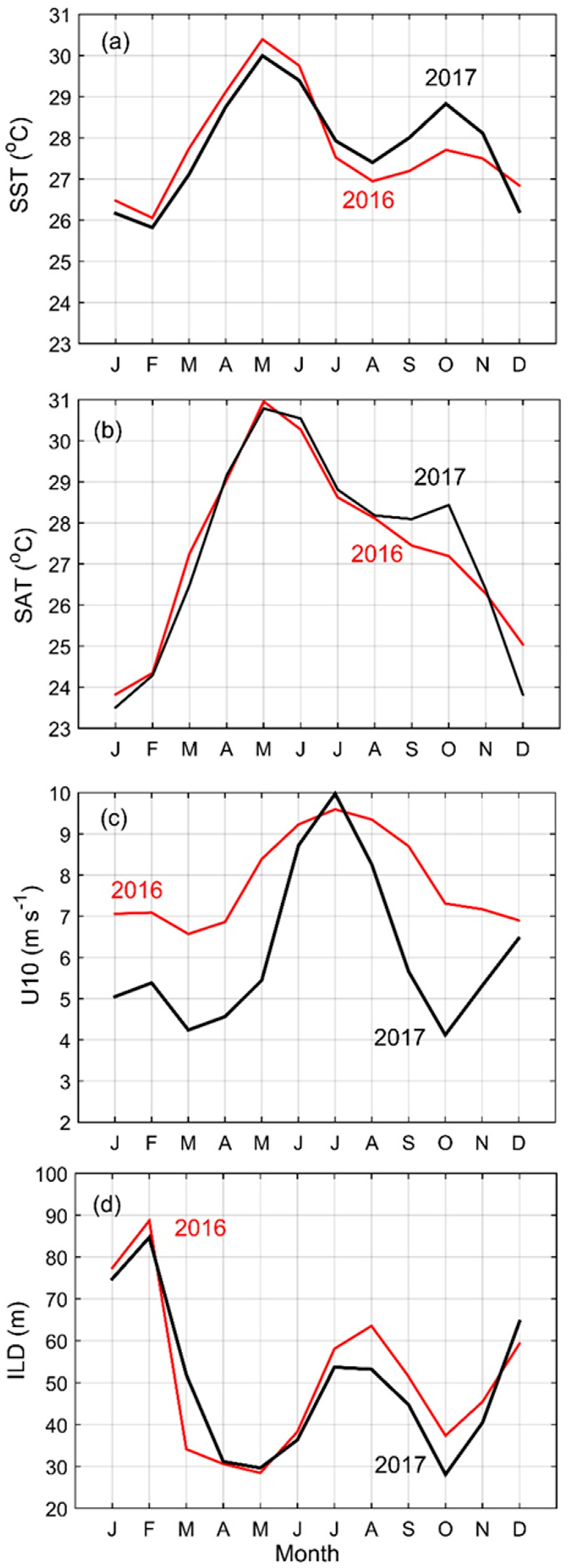
3.2.2. The Arabian Sea Region

The AS is a northwestern part of the TIO and has a monsoon climate. The strong seasonality of the SST is the result of the combined effects of oceanic and atmospheric processes at the air-sea interface (mainly controlled by seasonal changes in incoming solar radiation) and oceanic and atmospheric circulation. The annual cycle of monsoons mainly exhibits bimodal distribution and significantly affects the upper thermal structure, which is mainly responsible for regional circulation and heat/salt transport in the Arabian Sea [17]. The annual cycle of SST in the AS consists primarily of four stages: (1) a warming stage from about February to May; (2) cooling from May to August; (3) warming from August to October; and (4) cooling from October to January. This pattern is in contrast to the annual cycle of the SST in most other regions of the world ocean, which display only two phases: warming during pre-summer and summer; and cooling during autumn and winter. All available evidence suggests that this unusual behavior of the AS is due to the influence of the southwest monsoon (summer season) that dominates the AS during the northern hemispheric summer. The energetic circulation of wind during this period is known to have an effect on the SST. In the coastal regions, upwelling typically occurs, which brings up colder water and then spreads offshore [58], whereas in the open sea, the loss of energy and heat on the surface lowers the SST. These changes in SSTs and wind over the ocean may have an impact on the weather and climate of the adjacent landmasses [8,59].
The seasonal cycles of SST, SAT, wind speed and ILD over the AS in 2016 and 2017 are shown in Figure 10a–d, respectively. As shown in Figure 10a, the SST in this region experienced a semiannual cycle in SST circulation, where low SST occurred in both the summer and winter seasons. The winter minimum temperature reached 26 °C in February. However, the SST warmed during the pre-monsoon season and crossed 30 °C in May. It can be seen that SST was warmer by almost 4 °C. The SAT also peaked, reaching 31 °C in May (Figure 10b). The available climatology data suggest that the skies over the AS were clear prior to the onset of the summer monsoon, which means that it received a large amount of heat from solar radiation [60]. The winds were weak (Figure 10c) and therefore the latent heat loss was small, resulting in a large heat gain by the AS [61]. The pre-monsoon warming induced thermal stratification and suppressed turbulent mixing, causing the thermocline to rise with a shallow depth of isotherm layer (ILD < 30 m) in May (Figure 10d). In winter, the wind effect was weak compared to summer; convective mixing caused the cool surface waters to sink into a deeper layer, with larger ILD amplitude that reached 90 m in February. Interestingly, the seasonal cycle of SST distribution showed a slight increase in SST in 2016 as compared to 2017. This warming in the SST in 2016 may have been the result of large-scale atmospheric forcing linked to the presence of well-known strong El Niño conditions that appeared in the Pacific in early 2016, impacting the tropical Indian Ocean.
The summer monsoon in the AS expresses some of the strongest and most balanced wind forces. The period is characterized by strong winds, moist air, and a decrease in solar insulation due to cloud cover. The surface wind showed an increasing trend as the monsoon began (average wind speed reached 10 m s−1 in July 2017) and the summer minimum temperature dropped to around 27 °C in 2016 (versus 28 °C in 2017). This fall in SST during summer 2016 may be linked to the interannual variability of extreme negative IOD events that appeared in summer 2016 and impacted the western Indian Ocean with negative SST anomalies. Interestingly, mean SAT patterns were similar to SST but lower in amplitude—except for the monsoon season, in which most of the AS regions had SATs above 28 °C. During this period, the effect of wind force was high as compared to the pre-monsoon, and the turbulent mixing caused cool surface waters to sink into a deeper layer, resulting in a deeper thermocline. The average ILD reached 60 m in summer 2016 (Figure 10d).
A remarkable feature of the AS circulation is the existence of the strong upwelling along the Omani-Arabian coast that occurs during the summer season. A typical aspect of the upwelling mechanism is the presence of an undercurrent flowing opposite to the surface current [62]. The interesting element is that the cooling (or warming) of the SST occurs due to strong (or weak) upwelling variations that occur in the same region. The area of the undercurrent is characterized by isotherm downsloping at subsurface levels and upsloping of isotherms at surface levels toward the coast. It is important to mention here that the weak upwelling that occurs along the Omani-Arabian coast in summer usually affects and warms the SST, leading to an increased rainfall in the west coast of India and western BoB [18]. During pre-summer and summer seasons, SST in the western AS region is very sensitive to upwelling fluctuations due to the shallow mixed layer (~15–30 m) [16].
SST in the AS was cooler by almost 1 °C from July to October in 2016 (as compared to 2017). Cooling and warming of the SST is primarily due to strong or weak (respectively) upwellings that occur along the Omani-Arabian coast near the Ras al Hadd region between 22° N, 60° E band in late summer and early autumn in 2016 and 2017, respectively. In the upwelling, water of about 25 °C may have originated below the pycnocline. It was, therefore, colder than the surface water (which was 30 °C or more) and formed a shallow thermocline with reduced isothermal depth. This summer cooling in the northern AS caused dramatic changes in thermocline characteristics, where a small change in their strength might have a significant effect on the SST and hence on the monsoon precipitation [8,59]. The strong and weak upwellings can also be seen in Figure 5a,b, in which negative and positive SST anomalies prevailed along the Omani-Arabian coast in 2016 and 2017, respectively. During the 2016 monsoon season, high surface winds were noted in the AS, except in July (Figure 10c). The high wind speed increased the upwelling efficiency along the Omani-Arabian coast, forming a deep thermocline. In 2017, conversely, low surface winds were noted for the same period, and the lower wind speeds decrease the upwelling efficiency, forming a shallow thermocline. The depth of the thermocline varied from the sea surface, depending on multiple factors, including tide conditions and direction, the speed of coastal winds, and currents. These remarkable changes in SST in 2016 and 2017 (and their effect on summer precipitation in the BoB) were analyzed. The following section discusses that analysis.

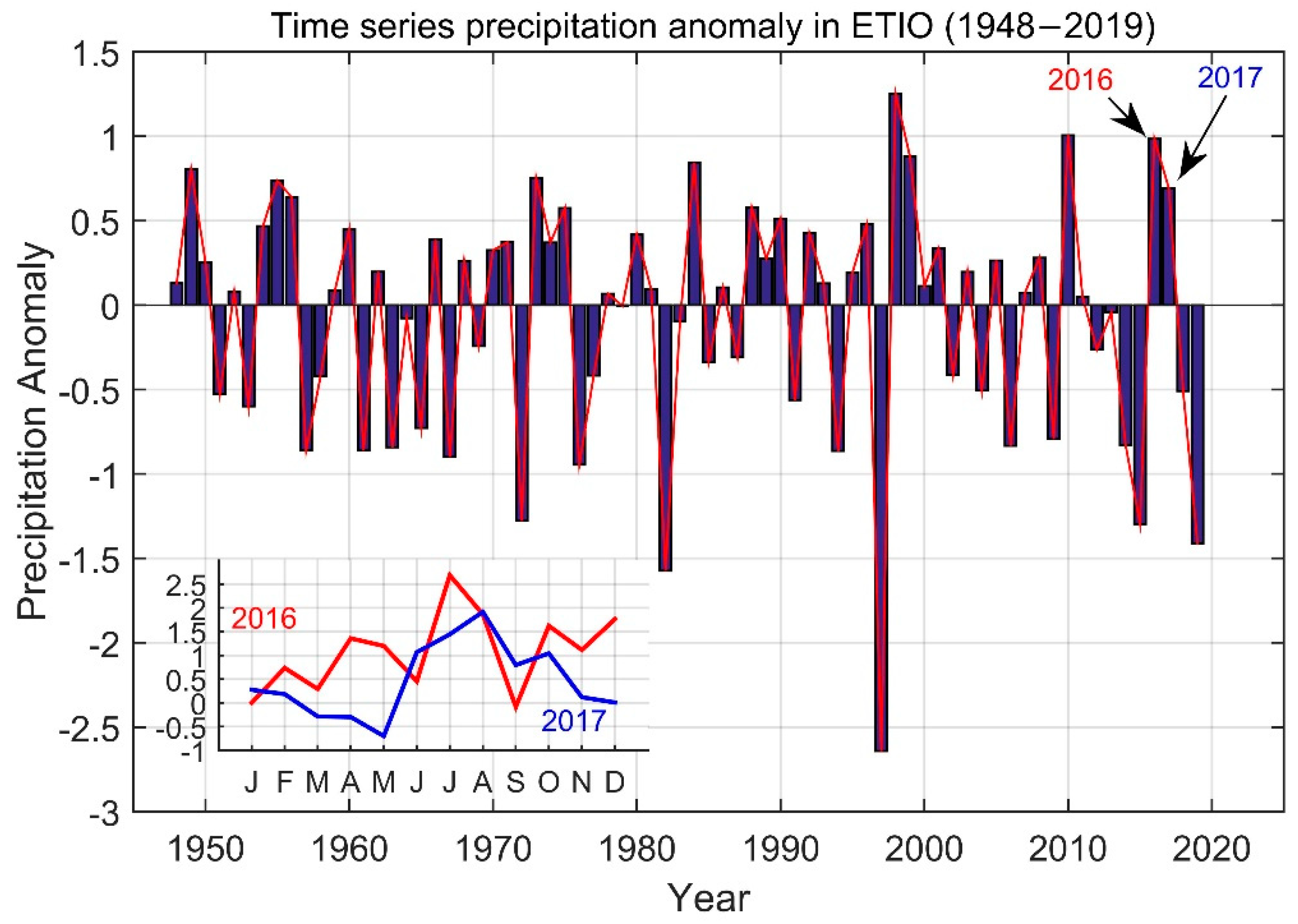
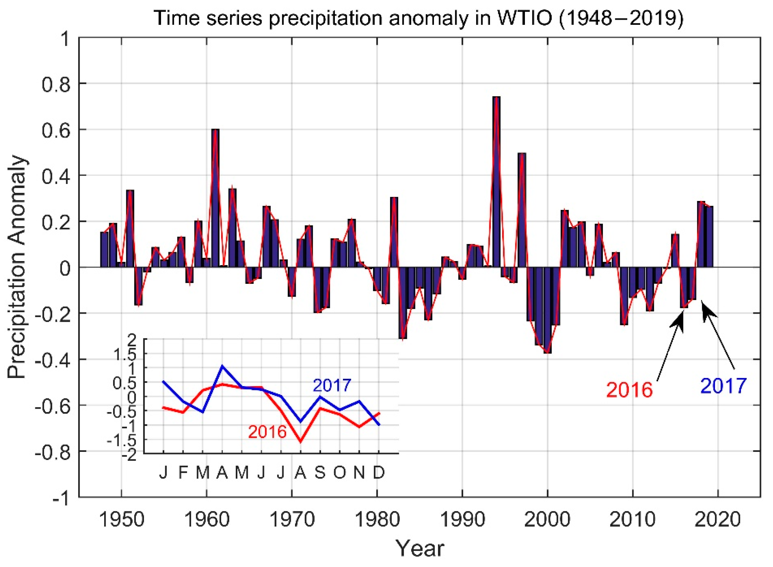
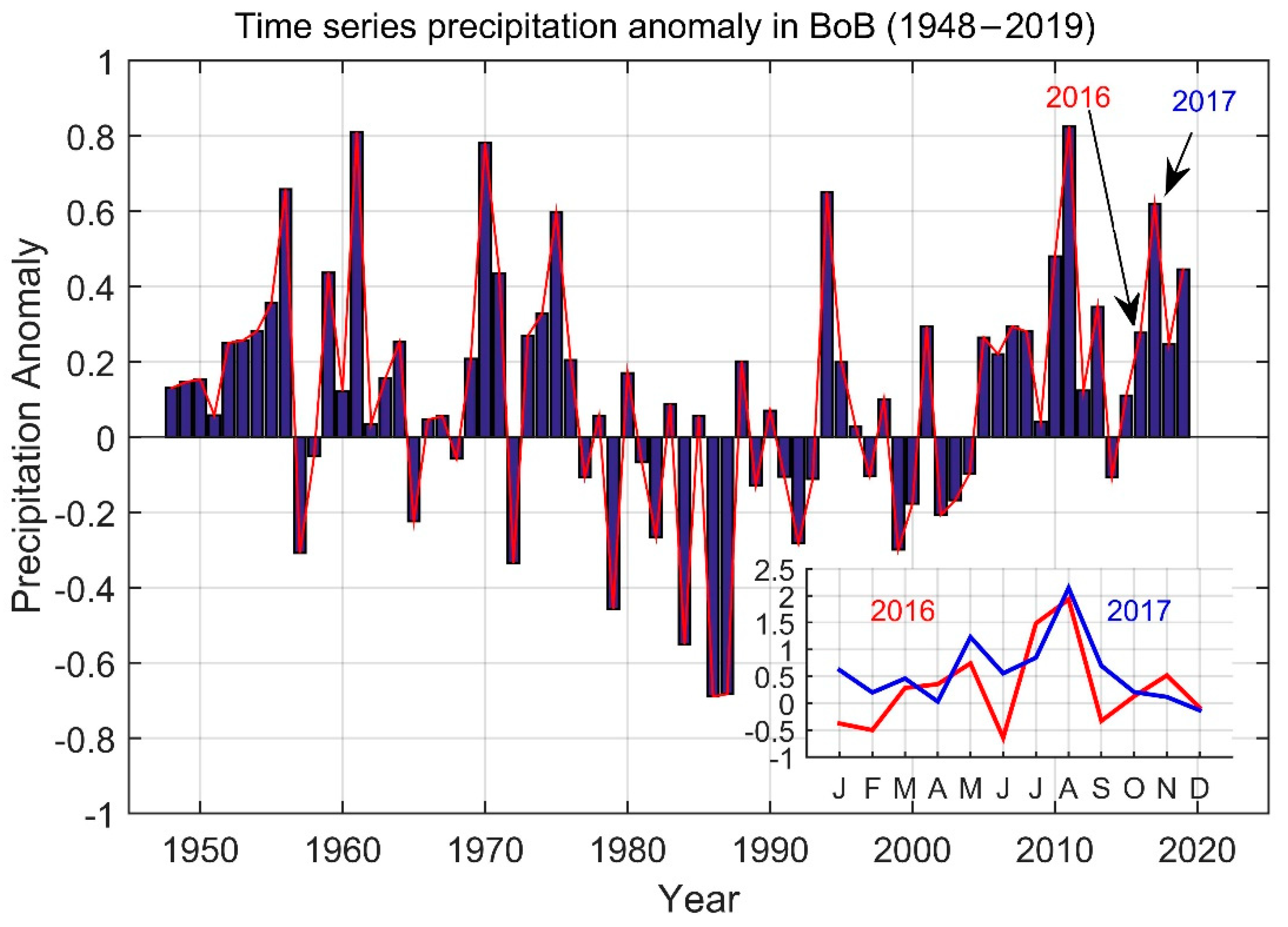
3.3. Precipitation Variability and SSS Circulation

As discussed earlier, SSTs in the Indian Ocean were significantly impacted by El Niño/La Niña phases in the Pacific Ocean, and by the evolution of the positive/negative IOD episodes in the tropical equatorial Indian Ocean in 2016–2017. During an El Niño, the Niño 3.4 region gets relatively warmer (as was observed until April in 2016). This may have an adverse impact on the Indian monsoon. In the late 1800s, Gilbert Walker investigated drought in India and determined that drought conditions were connected to shifts in ENSO. Several studies in the past have shown the relationship between SST in the TIO and the atmosphere in the surrounding regions [10,63,64,65,66]. Significant climatic impacts of extreme positive IOD events on severe East African floods have also been extensively studied [12,30,31]. According to a World Meteorological Organization report [29], the negative IOD event that occurred in June–September 2016 was associated with above average rainfall in many parts of Australia, Indonesia, and Bangladesh, as well as dry conditions in East Africa. On the other hand, there were significant weather and climate events in 2017, including dry conditions in summer in most of Australia, above average rainfall in the Horn of Africa late in the year after an extended period of drought, and monsoon floods in the Indian subcontinent [33]. This study further elucidated the impact of ENSO and IOD on precipitation variability in the Indian Ocean and surrounding areas in 2016 and 2017. As discussed in the previous section, the weak and strong upwellings that occurred along the Omani-Arabian coast led to respective warming and cooling in the SST, which affected precipitation and rainfall activity in the western coast of India and the BoB.
Time series of precipitation anomalies (1948–2019) in the WTIO, ETIO, and BoB regions are shown in Figure 11, Figure 12 and Figure 13, respectively. The BoB region is added to confirm the impact of the unusual warming and cooling in the SST on precipitation variability in 2016 and 2017. The monthly mean precipitation anomalies in 2016 and 2017 are presented within the figures. The climatology is based on a 20-year (1979–1998) reference period. The associated precipitation effects on SSS variability are shown in Figure 14. It became evident that the extreme El Niño in the Pacific during early 2016 directly affected rainfall distribution, with above normal rainfall over the ETIO and below normal rainfall over the WTIO. In the presence of El Niño, there was an excess in rainfall distribution that reached 10 mm d−1 (5 mm d−1) in February in the east pole (versus 5 mm d−1 in the west pole) (not shown). The associated drop in SSS in these regions is shown in Figure 14a,b. The low SSS during early 2016 in WTIO and ETIO may have been due to excessive precipitation over the evaporation.
Summer 2016 revealed a different variability with increased precipitation in the eastern pole of the tropical equatorial Indian Ocean, and reduced precipitation in the western pole. Excessive precipitation in the ETIO during the summer of 2016 may have been associated with the extreme negative IOD phase in June–August that triggered flooding in various parts of India, Nepal, and Bangladesh [29]. As shown in Figure 12, there was a decrease in precipitation in the WTIO during the summer and autumn of 2016. Below normal precipitation (<2 mm d−1) in June–October was mainly due to the strong negative IOD in 2016, which brought drought conditions in East Africa and reduced EASR (East African Short Rains) in October–December (not shown). Recently, Lu et al. 2018 [32] investigated the reduction of EASR by 1 mm d−1 in 2016, which included a 50% reduction in normal rainfall in some regions. Interestingly, the corresponding effect—low precipitation on surface salinity stratification—was not observed in the WTIO. Instead, there was a small decline in SSS in 2016 compared to 2017. The rise in surface salinity in 2017 is most likely due to high evaporation, which could have occurred due to a warmer SST in 2017 in the WTIO (Figure 5 and Figure 6). High evaporation adds more moisture to the atmosphere, contributing to the increased precipitation and flooding observed in East Africa by the end of 2017 [33].
In the AS region, the precipitation patterns were similar and no significant variations were noted over the entire period of 2016–2017 (not shown). However, the monthly average SSS remained high for the whole span of 2016 (compared to 2017) and was more pronounced in September (not shown). This was because SSTs in the AS covaried with the ONI observed in the Niño 3.4 region (5° S–5° N, 240–290° E). A positive SST anomaly was induced in the AS during the strong El Niño in the Pacific in 2016, which increased the evaporation rate and surface salinity due to fresh water loss.
In the BoB, warm SST anomalies persisted over the central region from January to May 2016 followed by the strong El Niño of 2016 (Figure 5a, the monthly variation is not shown). However, the effect of high SST on the surface salinity was not detected in this region (Figure 14c). Instead, there was a small decline in SSS (up to 0.5) from January to May in 2016, as compared to 2017. The dynamic behind this, however, could not be investigated in this study. As shown in Figure 13, precipitation patterns were almost identical in both years, with no significant differences except in June and September (in which positive precipitation anomalies were higher in 2017 than in 2016). The highest precipitation levels were observed during the monsoon season in both years, albeit with more in 2017. The corresponding effect—enhanced precipitation in the monsoon season—can be seen in Figure 14c, in which a slight decrease in SSS was observed in 2017, as compared to 2016. The low precipitation rate observed during the negative IOD and the high precipitation rate observed during the positive IOD in the BoB region are both consistent with the findings of Chanda et al. 2018 [67].

4. Conclusions

In 2016, the strong El Niño in the Pacific Ocean induced an extreme negative IOD in the Indian Ocean. The following year, a weak La Niña in the same region induced a weak positive IOD. These unusual events had a major impact on the SST and were followed by above-average flooding in the Indian subcontinent and drought conditions in East Africa [29,33]. The current study investigated the dynamics behind these events and their effect on SST variability in the TIO.
It was noted that during the strong El Niño in the Pacific in early 2016, the Indian Ocean warmed due to suppressed atmospheric convection and positive SST anomalies which persisted in both the east and west poles of the Equatorial Indian Ocean. Our analyses indicated that high SSTs along the Sumatran coast in the summer of 2016 induced local convection and western wind anomalies via the Bjerknes feedback mechanism [57]. These a led to an increase in wind speed and reduced SST in the western basin, leading to the east-west SST anomalies. The wind anomalies drove a series of Kelvin waves which reduced the upwelling efficiency and warmed the SST in the east. On the other hand, a weak positive IOD phase persisted throughout 2017; SST anomalies were below the 30-year average (reference period: 1981–2010) over the eastern pole and above the western pole of the equatorial Indian Ocean. The extreme El Niño also influenced rainfall distribution in the TIO. It was observed that, during El Niño, there was above normal rainfall over the ETIO, and below normal rainfall over the WTIO. The corresponding low sea surface salinity, found in the ETIO at the beginning of 2016, was mainly due to excess precipitation. The negative IOD in 2016 was characterized by above-average rainfall in Bangladesh and dry conditions in East Africa [29,32].
The strong El Niño and the extreme negative IOD also influenced the SST in the Arabian Sea region in 2016. It was observed that SST in the Arabian Sea remained high during early 2016 and decreased in the summer period, as compared to 2017. The increase in SST during early 2016 was mainly due to the strong El Niño, which warmed the Indian Ocean from January to May 2016. However, the summer SST in the western equatorial region of the Indian Ocean and the Arabian Sea was most likely reduced by the development of a negative IOD phase. Another important feature of this study was the observation of increased upwelling along the Omani-Arabian coast during the summer and post-summer periods of 2016—and the corresponding decreased upwelling in the same region in 2017. The low upwelling in 2017 warmed the SST by almost 1 °C, which increased precipitation rates in the BoB region. We found that, in the BoB region, precipitation was low during negative IOD and high during positive IOD, which is consistent with the findings of Chanda et al. in 2018 [67]. The SST variability is robust in the TIO in spite of the co-occurrence with the strong El Niño/La Niña cycle. The central role of the TIO in modulating the regional climate suggests that the variability of the SST in this basin has serious implications for both the highly populated regions around this basin and the ocean modeling community.

Author Contributions

Formal analysis, S.K. (Sartaj Khan) and Y.S; Funding acquisition, S.P. and Y.S; Methodology, S.K. (Sartaj Khan) and G.Z; Resources, S.P. and Y.S; Supervision, S.P. and Y.S; Validation, Y.S., G.Z. and D.B; Writing—original draft, S.K. (Sartaj Khan) and I.U.K.; Writing—review and editing, S.K. (Shazia Khan) I.U.K. and D.B. All authors have read and agreed to the published version of the manuscript.

Funding

This research received no external funding.

Institutional Review Board Statement

Not applicable.

Informed Consent Statement

Not applicable.

Acknowledgments

We would like to thank David Bradley and two anonymous reviewers for their insightful and constructive comments and suggestions. The authors also wish to acknowledge the Acoustic Science and Technology Laboratory of Harbin Engineering University for analysis and graphics. This work was supported by an international postgraduate scholarship awarded by the Chinese Scholarship Council (CSC) and National Key Research and Development Program of China, No. 2016YFC1400100.

Conflicts of Interest

The authors declare no conflict of interest.

References

  1. Dong, L.; McPhaden, M.J. Unusually warm Indian Ocean sea surface temperatures help to arrest development of El Niño in 2014. Sci. Rep. 2018, 8, 2249. [Google Scholar] [CrossRef]
  2. Kug, J.S.; Kang, I.S. Interactive feedback between ENSO and the Indian Ocean. J. Clim. 2006, 19, 1784–1801. [Google Scholar] [CrossRef]
  3. Okumura, Y.M.; Deser, C. Asymmetry in the duration of El Niño and La Niña. J. Clim. 2010, 23, 5826–5843. [Google Scholar] [CrossRef] [Green Version]
  4. Murtugudde, R.; Busalacchi, A.J. Interannual variability of the dynamics and thermodynamics of the tropical Indian Ocean. J. Clim. 1999, 12, 2300–2326. [Google Scholar] [CrossRef]
  5. Vinayachandran, P.N.; Iizuka, S.; Yamagata, T. Indian Ocean dipole mode events in an ocean general circulation model. Deep Sea Res. Part II 2002, 49, 1573–1596. [Google Scholar] [CrossRef]
  6. Walker, G.T. Correlation in seasonal variations of weather. IX. A further study of world weather. Mem. Indian Meteorol. Dep. 1924, 24, 275–332. [Google Scholar]
  7. Krishnamurthy, V.; Shukla, J. Intraseasonal and interannual variability of rainfall over India. J. Clim. 2000, 13, 4366–4377. [Google Scholar] [CrossRef]
  8. Arpe, K.; Dümenil, L.; Giorgetta, M.A. Variability of the Indian monsoon in the ECHAM3 model: Sensitivity to sea surface temperature, soil moisture, and the stratospheric quasi-biennial oscillation. J. Clim. 1998, 11, 1837–1858. [Google Scholar] [CrossRef]
  9. Keerthi, M.; Lengaigne, M.; Vialard, J.; de Boyer Montégut, C.; Muraleedharan, P. Interannual variability of the Tropical Indian Ocean mixed layer depth. Clim. Dyn. 2013, 40, 743–759. [Google Scholar] [CrossRef]
  10. Reverdin, G.; Cadet, D.L.; Gutzler, D. Interannual displacements of convection and surface circulation over the equatorial Indian Ocean. Q. J. R. Meteorol. Soc. 1986, 112, 43–67. [Google Scholar] [CrossRef]
  11. Saji, N.H.; Goswami, B.N.; Vinayachandran, P.N.; Yamagata, T. A dipole mode in the tropical Indian Ocean. Nature 1999, 401, 360–363. [Google Scholar] [CrossRef]
  12. Webster, P.J.; Moore, A.M.; Loschnigg, J.P.; Leben, R.R. Coupled ocean–atmosphere dynamics in the Indian Ocean during 1997–98. Nature 1999, 401, 356–360. [Google Scholar] [CrossRef] [PubMed]
  13. Murtugudde, R.; McCreary, J.P., Jr.; Busalacchi, A.J. Oceanic processes associated with anomalous events in the Indian Ocean with relevance to 1997–1998. J. Geophys. Res. Ocean. 2000, 105, 3295–3306. [Google Scholar] [CrossRef] [Green Version]
  14. Joseph, P.V. Monsoon variability in relation to equatorial trough activity over India and west Pacific Oceans. Mausam 1990, 41, 291–296. [Google Scholar]
  15. Niñomiya, K.; Kobayashi, C. Precipitation and moisture balance of the Asian summer monsoon in 1991. J. Meteorol. Soc. Jpn. 1999, 77, 77–99. [Google Scholar] [CrossRef] [Green Version]
  16. De Boyer Montégut, C.; Mignot, J.; Lazar, A.; Cravatte, S. Control of salinity on the mixed layer depth in the world ocean: 1. General description. J. Geophys. Res. Ocean. 2007, 112, C06011. [Google Scholar] [CrossRef]
  17. Murtugudde, R.; Seager, R.; Thoppil, P. Arabian Sea response to monsoon variations. Paleoceanography 2007, 22, PA4217. [Google Scholar] [CrossRef]
  18. Izumo, T.; Montégut, C.B.; Luo, J.J.; Behera, S.K.; Masson, S.; Yamagata, T. The role of the western Arabian Sea upwelling in Indian monsoon rainfall variability. J. Clim. 2008, 21, 5603–5623. [Google Scholar] [CrossRef] [Green Version]
  19. Suppiah, R. Relationships between Indian Ocean sea surface temperature and the rainfall of Sri Lanka. J. Meteorol. Soc. Jpn. 1988, 66, 103–112. [Google Scholar] [CrossRef] [Green Version]
  20. Kripalani, R.H.; Kumar, P. Northeast monsoon rainfall variability over south peninsular India vis-à-vis the Indian Ocean dipole mode. Int. J. Climatol. J. R. Meteorol. Soc. 2004, 24, 1267–1282. [Google Scholar] [CrossRef] [Green Version]
  21. Joseph, S.; Sahai, A.K.; Goswami, B.N. Eastward propagating MJO during boreal summer and Indian monsoon droughts. Clim. Dyn. 2009, 32, 1139–1153. [Google Scholar] [CrossRef] [Green Version]
  22. Joseph, S.; Sahai, A.K.; Chattopadhyay, R.; Sharmila, S.; Abhilash, S.; Rajeevan, M.; Mandal, R.; Dey, A.; Borah, N.; Phani, R. Extremes in June rainfall during the Indian summer monsoons of 2013 and 2014: Observational analysis and extended-range prediction. Q. J. R. Meteorol. Soc. 2016, 142, 1276–1289. [Google Scholar] [CrossRef]
  23. Trenberth, K.E.; Jones, P.D.; Ambenje, P.; Bojariu, R.; Easterling, D.; Klein Tank, A.; Parker, D.; Rahimzadeh, F.; Renwick, J.A.; Rusticucci, M.; et al. Chapter 3: Observations: Surface and atmospheric climate change. In Climate Change; Cambridge University Press: Cambridge, UK; New York, NY, USA, 2007; pp. 235–336. [Google Scholar]
  24. Venugopal, T.; Ali, M.M.; Bourassa, M.A.; Zheng, Y.; Goni, G.J.; Foltz, G.R.; Rajeevan, M. Statistical evidence for the role of southwestern Indian Ocean heat content in the Indian summer monsoon rainfall. Sci. Rep. 2018, 8, 12092. [Google Scholar] [CrossRef]
  25. Meehl, G.A.; Arblaster, J.M.; Fasullo, J.T.; Hu, A.; Trenberth, K.E. Model-based evidence of deep-ocean heat uptake during surface-temperature hiatus periods. Nat. Clim. Chang. 2011, 1, 360–364. [Google Scholar] [CrossRef]
  26. Brown, P.T.; Li, W.; Xie, S.-P. Regions of significant influence on unforced global mean surface air temperature variability in climate models. J. Geophys. Res. Atmos. 2015, 120, 480–494. [Google Scholar] [CrossRef] [Green Version]
  27. Dai, A.; Fyfe, J.C.; Xie, S.-P.; Dai, X. Decadal modulation of global surface temperature by internal climate variability. Nat. Clim. Chang. 2015, 5, 555–559. [Google Scholar] [CrossRef]
  28. McPhaden, M.J.; Zebiak, S.E.; Glantz, M.H. ENSO as an integrating concept in Earth science. Science 2006, 314, 1740–1745. [Google Scholar] [CrossRef] [Green Version]
  29. World Meteorological Organization (WMO). Statement on the State of the Global Climate in 2016; World Meteorological Organization: Geneva, Switzerland, 2017. [Google Scholar]
  30. Behera, S.K.; Krishnan, R.; Yamagata, T. Unusual ocean-atmosphere conditions in the tropical Indian Ocean during 1994. Geophys. Res. Lett. 1999, 26, 3001–3004. [Google Scholar] [CrossRef] [Green Version]
  31. Birkett, C.; Murtugudde, R.; Allan, T. Indian Ocean climate event brings floods to East Africa’s lakes and the Sudd Marsh. Geophys. Res. Lett. 1999, 26, 1031–1034. [Google Scholar] [CrossRef]
  32. Lu, B.; Ren, H.L.; Scaife, A.A.; Wu, J.; Dunstone, N.; Smith, D.; Wan, J.; Eade, R.; MacLachlan, C.; Gordon, M. An extreme negative Indian Ocean Dipole event in 2016: Dynamics and predictability. Clim. Dyn. 2018, 51, 89–100. [Google Scholar] [CrossRef]
  33. World Meteorological Organization (WMO). Statement on the State of the Global Climate in 2017; World Meteorological Organization: Geneva, Switzerland, 2018. [Google Scholar]
  34. Suthinkumar, P.S.; Babu, C.A.; Varikoden, H. Spatial Distribution of Extreme Rainfall Events during 2017 Southwest Monsoon over Indian Subcontinent. Pure Appl. Geophys. 2019, 176, 5431–5443. [Google Scholar] [CrossRef]
  35. Huang, B.; Liu, C.; Banzon, V.; Freeman, E.; Graham, G.; Hankins, B.; Smith, T.; Zhang, H.M. Improvements of the Daily Optimum Interpolation Sea Surface Temperature (DOISST) Version 2.1. J. Clim. 2020, 34, 2923–2939. [Google Scholar] [CrossRef]
  36. Banzon, V.; Smith, T.M.; Chin, T.M.; Liu, C.Y.; Hankins, W. A long-term record of blended satellite and in situ sea-surface temperature for climate monitoring, modeling and environmental studies. Earth Syst. Sci. Data 2016, 8, 165–176. [Google Scholar] [CrossRef] [Green Version]
  37. Reynolds, R.W.; Smith, T.M.; Liu, C.; Chelton, D.B.; Casey, K.S.; Schlax, M.G. Daily high-resolution-blended analyses for sea surface temperature. J. Clim. 2007, 20, 5473–5496. [Google Scholar] [CrossRef]
  38. Behringer, D.W.; Xue, Y. Evaluation of the global ocean data assimilation system at NCEP: The Pacific Ocean. In Proceedings of the Eighth Symposium on Integrated Observing and Assimilation Systems for Atmosphere, Oceans, and Land Surface, AMS 84th Annual Meeting, Washington State Convention and Trade Center, Seattle, WA, USA, 11–15 January 2004. [Google Scholar]
  39. Vissa, N.K.; Satyanarayana, A.N.V.; Prasad Kumar, B. Comparison of mixed layer depth and barrier layer thickness for the Indian Ocean using two different climatologies. Int. J. Climatol. 2013, 33, 2855–2870. [Google Scholar] [CrossRef]
  40. Adler, R.F.; Huffman, G.J.; Chang, A.; Ferraro, R.; Xie, P.P.; Janowiak, J.; Rudolf, B.; Schneider, U.; Curtis, S.; Bolvin, D.; et al. The version-2 global precipitation climatology project (GPCP) monthly precipitation analysis (1979–present). J. Hydrometeorol. 2003, 4, 1147–1167. [Google Scholar] [CrossRef]
  41. Huffman, G.J.; Adler, R.F.; Bolvin, D.T.; Gu, G. Improving the global precipitation record: GPCP version 2.1. Geophys. Res. Lett. 2009, 36, L17808. [Google Scholar] [CrossRef] [Green Version]
  42. Meissner, T.; Wentz, F.J.; Le Vine, D.M. The Salinity Retrieval Algorithms for the NASA Aquarius Version 5 and SMAP Version 3 Releases. Remote Sens. 2018, 10, 1121. [Google Scholar] [CrossRef] [Green Version]
  43. Huang, B.; Thorne, P.W.; Banzon, V.F.; Boyer, T.; Chepurin, G.; Lawrimore, J.H.; Menne, M.J.; Smith, T.M.; Vose, R.S.; Zhang, H.M. Extended reconstructed sea surface temperature, version 5 (ERSSTv5): Upgrades, validations, and intercomparisons. J. Clim. 2017, 30, 8179–8205. [Google Scholar] [CrossRef]
  44. Saji, N.H.; Yamagata, T. Structure of SST and surface wind variability during Indian Ocean Dipole mode year: COADS observations. J. Clim. 2003, 16, 2735–2751. [Google Scholar] [CrossRef]
  45. Rao, A.S.; Behera, S.K.; Masumoto, Y.; Yamagata, T. Interannual subsurface variability in the tropical Indian Ocean with a special emphasis on the Indian Ocean dipole. Deep Sea Res. Part II Top. Stud. Oceanogr. 2002, 49, 1549–1572. [Google Scholar] [CrossRef]
  46. Luo, J.J.; Masson, S.; Behera, S.; Yamagata, T. Experimental forecasts of the Indian Ocean Dipole using a coupled OAGCM. J. Clim. 2007, 20, 2178–2190. [Google Scholar] [CrossRef]
  47. Song, Q.; Vecchi, G.A.; Rosati, A.J. Predictability of the Indian Ocean sea surface temperature anomalies in the GFDL coupled model. Geophys. Res. Lett. 2008, 35, L02701. [Google Scholar] [CrossRef] [Green Version]
  48. Shi, L.; Hendon, H.H.; Alves, O.; Luo, J.J.; Balmaseda, M.; Anderson, D. How predictable is the Indian Ocean Dipole? Mon. Weather Rev. 2012, 140, 3867–3884. [Google Scholar] [CrossRef]
  49. Liu, H.; Tang, Y.; Chen, D.; Lian, T. Predictability of the Indian Ocean Dipole in the coupled models. Clim. Dyn. 2017, 48, 2005–2024. [Google Scholar] [CrossRef]
  50. Doi, T.; Storto, A.; Behera, S.K.; Navarra, A.; Yamagata, T. Improved prediction of the Indian Ocean dipole mode by use of subsurface ocean observations. J. Clim. 2017, 30, 7953–7970. [Google Scholar] [CrossRef]
  51. Ashok, K.; Guan, Z.; Yamagata, T. Impact of the Indian Ocean Dipole on the relationship between the Indian monsoon rainfall and ENSO. Geophys. Res. Lett. 2001, 28, 4499–4502. [Google Scholar] [CrossRef] [Green Version]
  52. Behera, S.K.; Luo, J.J.; Masson, S.; Rao, S.A.; Sakuma, H.; Yamagata, T. A CGCM study on the interaction between IOD and ENSO. J. Clim. 2006, 19, 1688–1705. [Google Scholar] [CrossRef]
  53. Reynolds, R.W.; Rayner, N.A.; Smith, T.M.; Stokes, D.C.; Wang, W. An improved in situ and satellite SST analysis for climate. J. Clim. 2002, 15, 1609–1625. [Google Scholar] [CrossRef]
  54. Weare, B.C. A statistical study of the relationships between ocean surface temperatures and the Indian monsoon. J. Atmos. Sci. 1979, 36, 2279–2291. [Google Scholar] [CrossRef]
  55. Lim, E.P.; Hendon, H.H. Causes and predictability of the negative Indian Ocean Dipole and its impact on La Niña during 2016. Sci. Rep. 2017, 7, 12619. [Google Scholar] [CrossRef] [PubMed] [Green Version]
  56. Kantha, L.H.; Clayson, C.A. An improved mixed layer model for geophysical applications. J. Geophys. Res. Ocean. 1979, 99, 25235–25266. [Google Scholar] [CrossRef]
  57. Bjerknes, J. Atmospheric teleconnections from the equatorial Pacific. Mon. Weather Rev. 1969, 97, 163–172. [Google Scholar] [CrossRef]
  58. Düing, W.; Leetmaa, A. Arabian Sea cooling: A preliminary heat budget. J. Phys. Oceanogr. 1980, 10, 307–312. [Google Scholar] [CrossRef]
  59. Shukla, J. Effect of Arabian sea-surface temperature anomaly on Indian summer monsoon: A numerical experiment with the GFDL model. J. Atmos. Sci. 1975, 32, 503–511. [Google Scholar] [CrossRef] [Green Version]
  60. Hastenrath, S.; Lamb, P. Climatic Atlas of the Indian Ocean. Part I. Surface Circulation and Climate; University of Wisconsin Press: Madison, WI, USA, 1979; p. 109. [Google Scholar]
  61. Rao, R.R.; Sivakumar, R. Seasonal variability of near-surface thermal structure and heat budget of the mixed layer of the tropical Indian Ocean from a new global ocean temperature climatology. J. Geophys. Res. Ocean. 2000, 105, 995–1015. [Google Scholar] [CrossRef]
  62. Yoshida, K.; Mao, H.L. A theory of upwelling of horizontal extent. J. Mar. Res. 1957, 16, 40–54. [Google Scholar]
  63. Saha, K. Zonal anomaly of sea surface temperature in equatorial Indian Ocean and its possible effect upon monsoon circulation. Tellus 1970, 22, 403–409. [Google Scholar] [CrossRef]
  64. Goddard, L.; Graham, N.E. Simulation skills of the SST-forced global climate variability of the NCEP-MRF9 and the Scripps-MPI ECHAM3 model. J. Clim. 1999, 13, 3657–3679. [Google Scholar]
  65. Nicholls, N. All-India summer monsoon rainfall and sea surface temperatures around northern Australia and Indonesia. J. Clim. 1995, 8, 1463–1467. [Google Scholar] [CrossRef]
  66. Nicholson, S.E.; Kim, J. The relationship of the El Niño–Southern oscillation to African rainfall. Int. J. Climatol. J. R. Meteorol. Soc. 1997, 17, 117–135. [Google Scholar] [CrossRef]
  67. Chanda, A.; Das, S.; Mukhopadhyay, A.; Ghosh, A.; Akhand, A.; Ghosh, P.; Ghosh, T.; Mitra, D.; Hazra, S. Sea surface temperature and rainfall anomaly over the Bay of Bengal during the El Niño-Southern Oscillation and the extreme Indian Ocean Dipole events between 2002 and 2016. Remote Sens. Appl. Soc. Environ. 2018, 12, 10–22. [Google Scholar] [CrossRef]
Figure 1. Yearly mean SST anomalies of world oceans in 2016 (a) and 2017 (b). The black boxes correspond to the Niño 3.4 area (5° S–5° N, 240–290° E) in the East Pacific Ocean. Monthly average SST anomalies in Niño 3.4 region are shown within the map.
Atmosphere 12 00587 g001
Figure 2. Geographical extent of the TIO (23.5° S–23.5° N, 30–120° E). The black boxes represent the areas of study: ETIO (10° S–Eq, 90–110° E), WTIO (10° S–10° N, 50–70° E), AS (12–24° N, 55–75° E), and BoB (10–20° N, 80–100° E). The BoB region is included in this study for analysis of precipitation variability.
Atmosphere 12 00587 g002
Figure 3. Time series of the ENSO index and SST anomalies in Niño 3.4 Region. Warm and cold periods are based on a threshold of +/−0.5 °C for the ONI (3 month running mean of SST anomalies in the Niño 3.4 Region) and represented by red and blue colors, respectively. Dotted lines represent standard deviations of the series. The 2015–2016 El Niño was the first powerful El Niño of the 21st century and one of the three strongest El Niño events since 1950.
Atmosphere 12 00587 g003
Figure 4. Time series of average SST anomalies in the (a) ETIO (10° S–Eq, 90–110° E), (b) WTIO (10° S–10° N, 50–70° E), and (c) IOD index (DMI=WTIO−ETIO). Data were derived from Extended Reconstructed Sea Surface Temperature version 5 (ERSST.V5) from 1990 to 2020. The red arrows indicate that negative IOD events occurred during El Niño. The weak positive IOD event in 2017 is indicated by black arrow.
Atmosphere 12 00587 g004
Figure 5. Evolution of SST anomalies (°C) in the TIO in 2016 and 2017 with respect to 1981–2010 reference period, (a) yearly mean of SST anomalies in 2016, (b) yearly mean of SST anomalies in 2017. The monthly distribution of SST anomalies in 2016 and 2017 is shown within the map. The two boxes represent WTIO (10° S–10° N, 50–70° E) and ETIO (10° S–Eq, 90–110° E). Data obtained from NOAA OISSTv2.1.
Atmosphere 12 00587 g005
Figure 6. Yearly mean SST in the TIO based on NOAA OISSTv2.0 for 2016 (a) and 2017 (b). Monthly mean SST cycle of the WTIO and ETIO regions is depicted on the map.
Atmosphere 12 00587 g006
Figure 7. As in Figure 6, but for isothermal layer depth (ILD) in 2016 (a) and 2017 (b). The changes in the thermocline depth are reflected by the changes in the ILD. Data obtained from GODAS.
Atmosphere 12 00587 g007
Figure 8. As in Figure 6, but for neutral wind speed at 10 m above sea surface (U10) in 2016 (a) and 2017 (b). Data provided by the WHOI OAFlux project.
Atmosphere 12 00587 g008
Figure 9. Monthly mean SAT variability at 1 atmospheric pressure in the equatorial tropical Indian Ocean in 2016 (a) and 2017 (b). Data provided by NCEP Global Data Assimilation System (GDAS) and available at 2.5° × 2.5° horizontal resolution.
Atmosphere 12 00587 g009
Figure 10. Monthly mean (a) sea surface temperature (SST), (b) sea air temperature (SAT) at 1 atmospheric pressure, (c) neutral wind at 10 m above sea surface (U10), and (d) isothermal layer depth (ILD) in the Arabian Sea region (12–24° N, 50–75° E) during 2016 and 2017.
Atmosphere 12 00587 g010
Figure 11. Time series (1948–2019) of precipitation anomalies in the ETIO region. Datasets provided by NOAA precipitation reconstruction (PREC). The climatology is based on a time period covering 1979–1998. The monthly distribution of precipitation anomalies in 2016 and 2017 is shown within the figure.
Atmosphere 12 00587 g011
Figure 12. As in Figure 11, but for WTIO region.
Atmosphere 12 00587 g012
Figure 13. As in Figure 11, but for BoB region.
Atmosphere 12 00587 g013
Figure 14. SSS variability in the TIO in the areas under investigation during 2016 and 2017: (a) ETIO (10° S–Eq, 90–110° E), (b) WTIO (10° S–10° N, 50–70° E), and (c) BoB (10–20° N, 80–100° E). Data obtained from the SMAPv3 (Soil Moisture Active Passive version 3).
Atmosphere 12 00587 g014
Publisher’s Note: MDPI stays neutral with regard to jurisdictional claims in published maps and institutional affiliations.

