Water Quality Prediction in the Luan River Based on 1-DRCNN and BiGRU Hybrid Neural Network Model

Abstract

The current global water environment has been seriously damaged. The prediction of water quality parameters can provide effective reference materials for future water conditions and water quality improvement. In order to further improve the accuracy of water quality prediction and the stability and generalization ability of the model, we propose a new comprehensive deep learning water quality prediction algorithm. Firstly, the water quality data are cleaned and pretreated by isolation forest, the Lagrange interpolation method, sliding window average, and principal component analysis (PCA). Then, one-dimensional residual convolutional neural networks (1-DRCNN) and bi-directional gated recurrent units (BiGRU) are used to extract the potential local features among water quality parameters and integrate information before and after time series. Finally, a full connection layer is used to obtain the final prediction results of total nitrogen (TN), total phosphorus (TP), and potassium permanganate index (COD-Mn). Our prediction experiment was carried out according to the actual water quality data of Daheiting Reservoir, Luanxian Bridge, and Jianggezhuang at the three control sections of the Luan River in Tangshan City, Hebei Province, from 5 July 2018 to 26 March 2019. The minimum mean absolute percentage error (MAPE) of this method was 2.4866, and the coefficient of determination (R²) was able to reach 0.9431. The experimental results showed that the model proposed in this paper has higher prediction accuracy and generalization than the existing LSTM, GRU, and BiGRU models.

1. Introduction

With the rapid development of China’s economy and science and technology, people’s production and living range is more and more extensive. Domestic sewage, industrial wastewater, and farmland drainage all contain a large amount of nitrogen, phosphorus, and other inorganic salts. The content of total nitrogen (TN), total phosphorus (TP), and potassium permanganate (COD-Mn) in the water body has greatly increased. These factors are the main reasons for water eutrophication [1]. The deterioration of river water quality has a profound impact on the ecological health of surface water and its tributaries, which undoubtedly increases the burden of sustainable development of human drinking water. In the stage of water environment treatment, real-time prediction of water quality can provide a scientific decision-making basis for the protection and treatment of the water environment. Therefore, the establishment of an effective water quality parameter prediction model is of great significance for improving the water quality of the river [2].

At present, the water quality prediction models can be divided into two categories according to their intrinsic properties: mechanism and non-mechanism (data-driven) water quality prediction models. The mechanism model is constrained by physical, biological, chemical, and other factors of the water environment system, and is derived from the system structure data. From the earliest Streeter–Phelos (S-P) model system, QUAL model system [3], to WASP model system [4], and BASINS model system [5] in recent years, as well as the secondary development based on the above original models, good application effects have been achieved. However, these models need more basic materials and data, and the foundation construction is more complicated. Due to being not fully aware of the detailed mechanism changes of many water environment systems in China, we find it difficult to describe the trend of water quality accurately by mechanism modeling.

Most data-driven models have significant effects on the prediction of water quality parameters. The major methods are the time series method, the gray theory prediction method [6], the regression prediction method (such as support vector machine) [7], and the artificial neural network prediction method [8]. However, the first three methods have some defects, such as poor generalization ability, low calculation accuracy, and low prediction accuracy. In recent years, the deep learning method has attracted more and more attention in water quality modeling. Artificial neural network (ANN) is a kind of machine learning technology that is realized by the extensive parallel interconnection of self-adaptive simple units to simulate the biological nervous system. It is the basis of deep learning, and it has the advantages of good robustness and the ability to fully fit complex nonlinear relationships [9]. In 2015, Kim et al. [10] combined the data clustering method and the back propagation neural network (BPNN) to establish a prediction model of the five water quality parameters of pH, dissolved oxygen (DO), turbidity (Turb), total nitrogen (TN), and total phosphorous (TP). Rahim Barzegar et al. [11] used the wavelet neural network (GWNN) to predict the salt concentration of the Aji Chay River in northwest Iran in 2016. Through the calibration and verification of the model, the superiority of GWNN in water quality prediction was found. Liu et al. [12] established a water temperature prediction model based on the combination of empirical mode decomposition (EMD) and the BPNN.

The water quality data are time series data composed of water quality parameters collected at different times, used to describe the change of water quality status with time. They reflect the state and characteristic that water quality parameters change periodically with time, but the above model lacks the mechanism to process time data. In response to the above problems, Long et al. [13] proposed a general-purpose initialized attention residual network (IARN) water supply prediction model. In [14], the authors developed a water quality prediction model combining kernel principal component analysis (KPCA) and recurrent neural network (RNN) model to predict the variation trend of dissolved oxygen (DO), which not only reduced the noise of the original sensory data, but also retained the operational information, having the performance of processing time-series data. Still, the traditional RNN can only capture short-term memory due to the disappearance of the gradient. The long short-term memory (LSTM) network combines short-term memory and long-term memory through subtle gate control and solves the problem of gradient disappearance to a certain extent. It is suitable for processing and predicting important events with long intervals and delays in corresponding time series. Subsequently, the gated recurrent unit (GRU) method [15] was first proposed in 2014, which is a variant of the long-term and short-term memory network LSTM. It has fewer parameters and faster convergence speed under the condition of the same prediction accuracy as LSTM [16]. In recent years, GRU has achieved good application results in fields of time series data prediction such as meteorology [17], wind power [18], and pond aquaculture water [19]. To efficiently integrate relevant information in the context of time series data, Liu Juntao [20] and other scholars have successfully applied the bidirectional stacked simple recursive unit (Bi–S–SRU) to water quality prediction of marine aquaculture, demonstrating the feasibility of bidirectional neural network to predict water quality parameters. Aiming at the problem of PM2.5 air pollution prediction, Qing et al. [21] adopted a new hybrid algorithm of one-dimensional convolution neural network (1-DCNN) and bi-directional gated recurrent units (BiGRU), which fully excavated the local characteristics of meteorological data from different sources. Reference [22] proposed a 1-DCNN model to predict the trend of Bitcoin, and experimental results showed that the algorithm can predict the trend of Bitcoin more accurately than the LSTM model. At the same time, [23] envisaged a residual expansion causal convolution neural network (Res-DCCNN) with nonlinear concerns for multi-step wind speed prediction. Similarly, the residual convolutional neural network (RCNN) has been applied to many fields, such as removing electroencephalogram (EEG) signal noise [24] and extracting Wi-Fi signal spatial features [25]. On the other hand, the innovative two-way depth network and residual network framework have not been involved in the field of water quality prediction.

In this paper, we proposed a new hybrid neural network model that combines one-dimensional residual convolutional neural networks (1-DRCNN) with BiGRU, focusing on learning the potential local features of water quality time series data and capturing contextual time attribute. Then, the indexes of total nitrogen, total phosphorus, and potassium permanganate in the Daheiting reservoir, Luanxian bridge, and Jianggezhuang section of Luanhe River were predicted, respectively. Finally, the experimental results were compared with BiGRU, GRU, and LSTM single models, and the efficiency, accuracy, and stability of each method are discussed and evaluated on the basis of the real value.

2. Materials and Methods

2.1. Study Area and Monitoring Data

The Luan River Basin is located between 115°30′~118°45′ E and 39°10′~42°40′ N, with a length of 500 km from north to south and an average width of 90 km from east to west. The widest part upstream is 1175 m, and the narrowest part downstream is 12 m, with a drainage area of 4480 km². The Luan River flows into Chengde city through Fengning County, Hebei Province, and then into the Bohai Sea in Leting County, Tangshan City, with a total length of 877 km. The Luan River, the second-longest river in Hebei Province, is the main water source in the north and east of Hebei Province, as well as an important water source for Tianjin City.

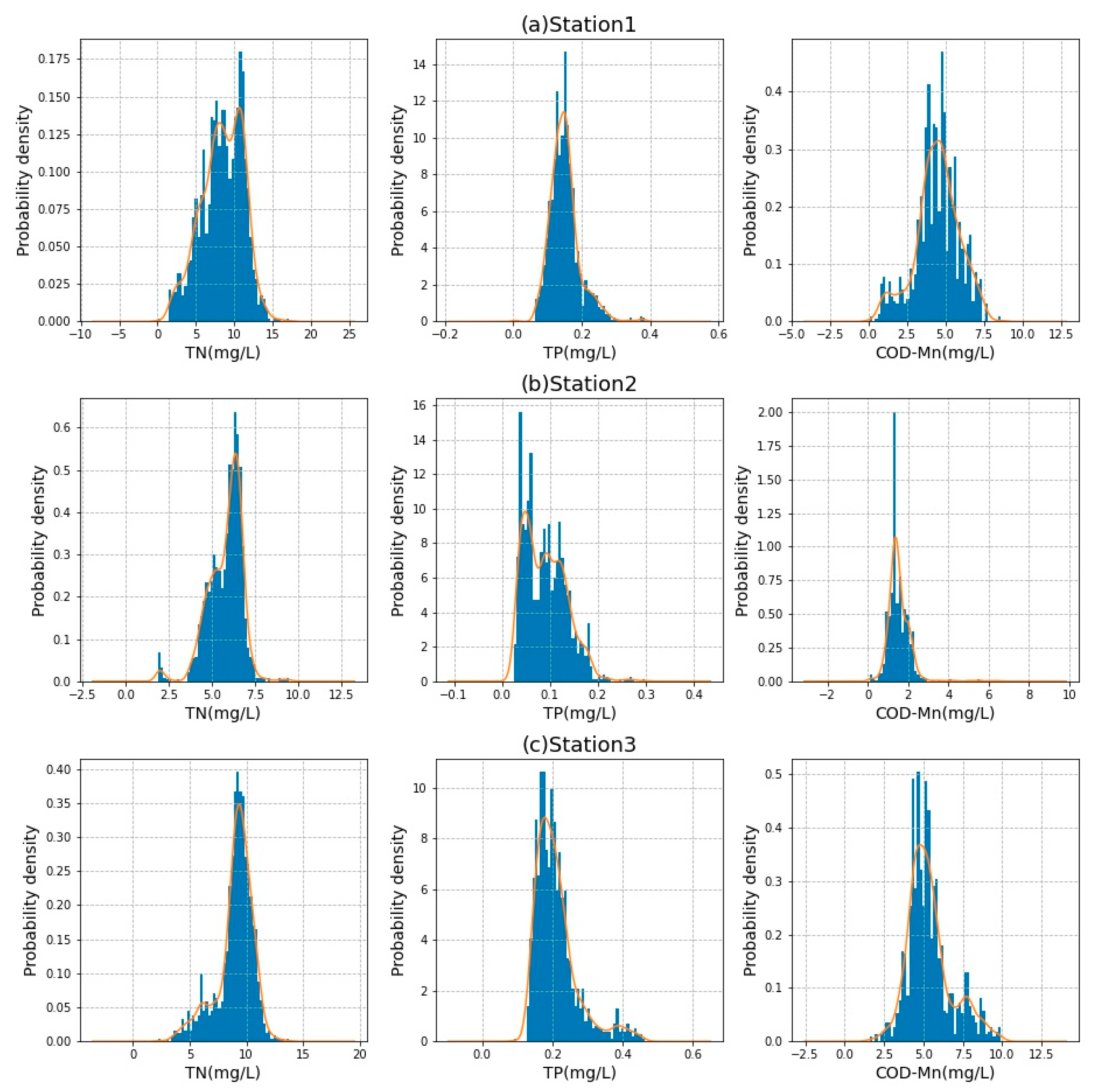
The data in this paper is from three sections of the Luan River monitored by the automatic water quality monitoring station in Tangshan city, Hebei Province, China, from 5 July 2018 to 26 March 2019, namely, Daheiting reservoir, Luanxian bridge, and Jianggezhuang. The automatic monitoring station uses the automatic positioning cruise system of an unmanned surface vehicle (USV) to locate the position of the cross-section and uses the data acquisition module to collect experimental data every 4 hours, and then uses the transmission module and cloud service module for data transmission and cloud storage, respectively [26,27]. The alternative names, data volume, and location information of the monitoring sections are listed in

Table 1. Monitoring cross-section name and location.

Alternative Name	Cross-Section Name	Number of Data	Location
			Longitude	Latitude
Station 1	Daheiting Reservoir	1360	118°18′16.1748″ E	40°13′5.3292″ N
Station 2	Luanxian Bridge	1360	118°46′24.8″ E	39°45′30.24″ N
Station 3	Jianggezhuang	1360	119°8′33.738″ E	39°27′48.024″ N

. These mainly include 9 water quality parameters: temperature (T, °C), pH, dissolved oxygen (DO, mg/L), biochemical oxygen demand (BOD, mg/L), turbidity (NTU), potassium permanganate index (COD-Mn, mg/L), ammonia nitrogen (NH4-N, mg/L), total phosphorus (TP, mg/L), and total nitrogen (TN, mg/L). Since TN, TP, and COD-Mn are the criteria for evaluating the eutrophication of the water body, this study mainly predicted the above three parameters and drew probability density distribution, as shown in Figure 1. It can be observed from Figure 1 that the distribution of the water quality data used in this paper was the relatively concentrated and approximately normal distribution.

2.2. Data Cleaning

The water quality data used in this article came from different collection equipment at the cross-section automatic monitoring station. Due to factors such as failure of the equipment or human error records, the water quality data will inevitably have outliers and vacancies. These non-compliant data will cause the algorithm to incorrectly capture the development direction of the predicted value, resulting in lower accuracy of the model [28]. Therefore, before the predictive model is constructed, the data set must be cleaned. In this paper, the isolation forest and Lagrange interpolation methods were used to revise the water quality data.

2.2.1. Isolation Forest

Qin et al. [29] used the improved isolation forest to effectively detect the outliers of the measured data of the Chu River Basin in 2019, which shows that this algorithm can correctly identify the outliers in hydrological data. Isolation forest is an unsupervised anomaly detection method suitable for continuous numerical data [30]. The core version is to segment the dataset recursively without considering the distance or density of the two samples until all the sample points are isolated, and the outliers are closer to the root. Outlier detection is mainly divided into two stages:

In the first stage, the establishment of iForest:

• ψ sample points are randomly selected from the training data as sample subset and put into the root node.
• Randomly specify a dimension or feature and generate a cutting point P between the maximum and minimum value of the current node data.
• A hyperplane is generated by this cutting point, and the current node data space is divided into two subspaces. Data less than P are placed in the specified dimension on the left child of the current node, and data greater than or equal to P are placed on the right child of the current node.
• Recursively execute steps (2) and (3) in the child nodes, and constantly build new child nodes until only one datum in the child nodes cannot be further divided or the child nodes have reached the limit height.
• Repeat steps (1) to (4) until t iTrees are generated to form the iForest.

In the second stage, calculate the anomaly score: it is used to determine outliers. The closer the outlier score is to 1, the more likely the node is to be an outlier.

Given the sample subspace of size n, the outlier score of sample X is defined as:

$$\mathrm{Score}\left(\mathrm{X},\mathrm{n}\right)=2^{-\frac{\mathrm{E}\left(\mathrm{h}\left(\mathrm{X}\right)\right)}{\mathrm{C}\left(\mathrm{n}\right)}}$$

(1)

$$\mathrm{C}\left(\mathrm{n}\right)=2\mathrm{H}\left(\mathrm{n}-1\right)-\frac{2\left(\mathrm{n}-1\right)}{\mathrm{n}}$$

(2)

where H(n − 1) is a harmonic function, which can be estimated by ln(n − 1) + 0.5772156649; C(n) is the average path length of the binary tree constructed with n sample data; and E(h(X)) is the average path length of data X in multiple iTree.

2.2.2. Lagrange Interpolation Method

The Lagrange interpolation method gives the nodal basis functions at the node $\mathrm{x}$ and then makes a linear combination of the basis functions, and the nodal function is used as the combination coefficient. Obtain the vacant node functions according to the non-vacant node functions and realize the filling of the vacant values. From this, the formula of Lagrange interpolation polynomial is obtained:

$${\mathrm{L}}_{\mathrm{n}}\left(\mathrm{x}\right)={\mathrm{y}}_0{\mathrm{l}}_0\left(\mathrm{x}\right)+{\mathrm{y}}_1{\mathrm{l}}_1\left(\mathrm{x}\right)+\dots +{\mathrm{y}}_{\mathrm{n}}{\mathrm{l}}_{\mathrm{n}}$$

(3)

$${\mathrm{l}}_{\mathrm{i}}\left(\mathrm{x}\right)=\begin{array}{c}\mathrm{n}\\ \prod \\ \mathrm{i}=0,\mathrm{i}\ne \mathrm{j}\end{array}\frac{\mathrm{x}-{\mathrm{x}}_{\mathrm{i}}}{\mathrm{x}-{\mathrm{x}}_{\mathrm{j}}}$$

(4)

where ${\mathrm{y}}_{\mathrm{n}}$ is the combination coefficient and ${\mathrm{l}}_{\mathrm{i}}\left(\mathrm{x}\right)$ is the interpolation function.

2.3. One-Dimensional Residual Convolutional Neural Networks

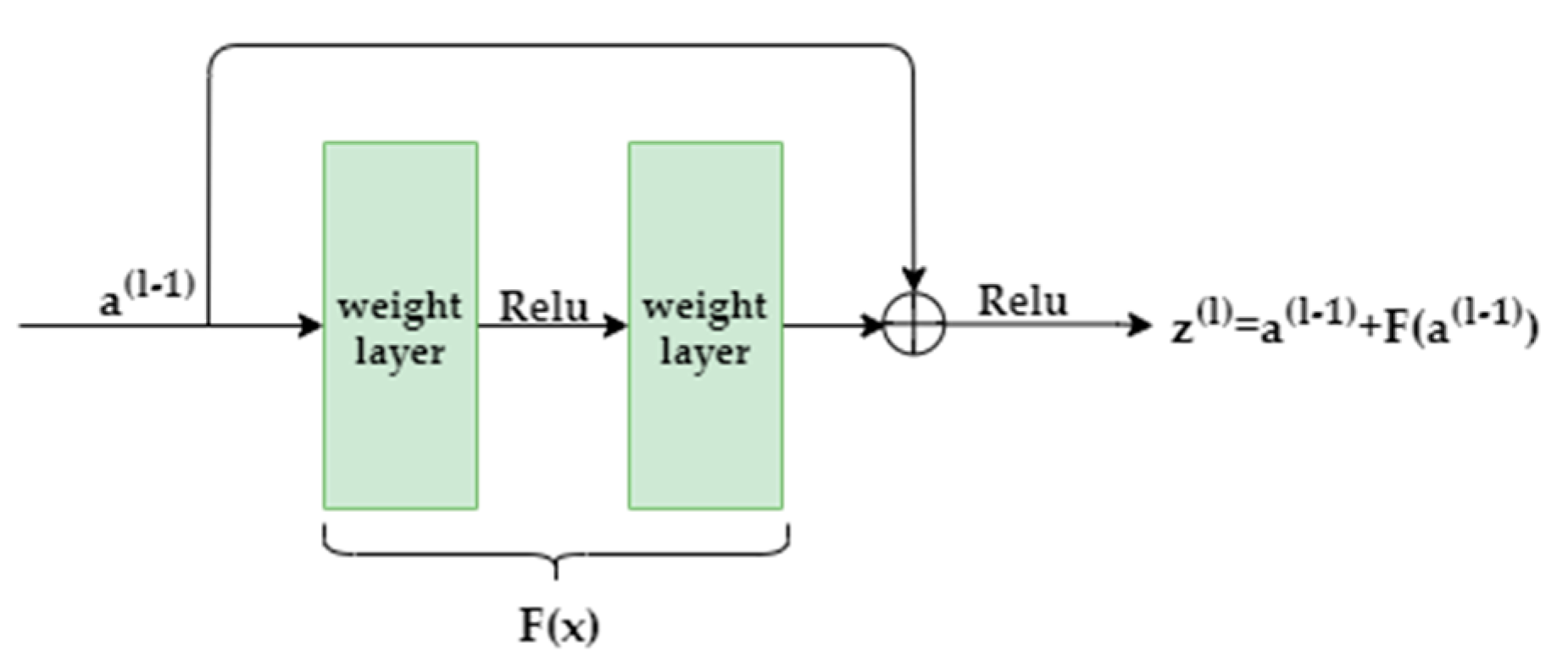
Since the water environment system is a complex and changeable nonlinear system, there are different and unknown correlations between the parameters. In order to reduce the impact of water environment signal noise on water quality prediction, we used the good feature extraction and expression capabilities of the convolution neural network (CNN) to extract potential features from water quality data. However, in terms of the traditional long and deep CNN in the process of model training, as the network deepens, the training accuracy will reach saturation and then rapidly decline [31]. Aiming to solve the above problems, He et al. [30] proposed a residual convolutional neural network in 2016, in which the main idea was to introduce residual learning and implement it in the form of the residual block.

Since the identity mapping in the neural network will not produce over-fitting, the residual block realizes the natural identity mapping $\mathrm{H}\left({\mathrm{a}}^{\left(\mathrm{l}-1\right)}\right)\to {\mathrm{a}}^{\left(\mathrm{l}-1\right)}$ in the form of layer jumping connection, which is equivalent to the residual part $\mathrm{F}\left({\mathrm{a}}^{\left(\mathrm{l}-1\right)}\right)$ approaching 0, as shown in Figure 2.

The internal structure of the residual block is mainly composed of batch-normalized layers (BN), one-dimensional convolutional layers (1-D Conv layer), and activation functions [24].

BN layer: BN layer calculates the first-order and second-order statistics of each batch, and constantly adjusts the intermediate output of the evolution layer of one-dimensional convolutional neural networks (1-DCNN) so that the high-level network can adapt to the parameter update of the low-level network, and the output of each layer tends to be stable, avoiding the phenomenon that the gradient vanishing of the high-level network leads to the decrease of the convergence speed of the network [32].

1-D Conv layer: The convolution layer of 1-DCNN uses the convolution kernel with the same weight and different local regions of one-dimensional signal to carry out convolution operation, learning the specific features of input data with all positions, and then generates the corresponding one-dimensional feature mapping. The output ${\mathrm{y}}_{\mathrm{k}}^{\mathrm{l}}$ of each convolution layer is

$${\mathrm{y}}_{\mathrm{k}}^{\mathrm{l}}=\mathrm{f}\left({\mathrm{x}}_{\mathrm{i}}^{\mathrm{l}}\right)$$

(5)

$${\mathrm{x}}_{\mathrm{i}}^{\mathrm{l}}={{\displaystyle \sum }}_{\mathrm{i}=1}^{{\mathrm{N}}_{\mathrm{l}-1}}\mathrm{conv}\left({\mathrm{w}}_{\mathrm{ik}}^{\mathrm{l}-1},{\mathrm{a}}_{\mathrm{i}}^{\mathrm{l}-1}\right)+{\mathrm{b}}_{\mathrm{k}}^{\mathrm{l}}$$

(6)

$$\mathrm{f}\left(\mathrm{x}\right)=\mathrm{SELU}=\mathsf{\beta }\max \left({\mathsf{\alpha }\mathrm{e}}^{\mathrm{zx}}-\mathsf{\alpha },\mathrm{x}\right)$$

(7)

where ${\mathrm{x}}_{\mathrm{i}}^{\mathrm{l}}$ is the input of the ${\mathrm{i}}^{\mathrm{th}}$ neuron of the layer l network, ${\mathrm{a}}_{\mathrm{k}}^{\mathrm{l}-1}$ is the output of the ${\mathrm{i}}^{\mathrm{th}}$ neuron of the layer l-1 network, ${\mathrm{w}}_{\mathrm{ik}}^{\mathrm{l}-1}$ is the filter between the ${\mathrm{k}}^{\mathrm{th}}$ neuron of the layer l-1 network and the ${\mathrm{i}}^{\mathrm{th}}$ neuron of the layer l network, and ${\mathrm{b}}_{\mathrm{k}}^{\mathrm{l}}$ is defined as the bias of the ${\mathrm{k}}^{\mathrm{th}}$ neuron of the layer l network. For the feature expression ability of the convolution layer to be improved, an activation function f (.) is needed to realize the nonlinear feature mapping of the convolution layer. In this paper, the Selu activation function was selected and expressed by Equation (6). Among them, α and β are constant values; β = 1.05070098 and α = 1.67326324, respectively [33].

2.4. Bi-Directional Gated Recurrent Unit

The gated recurrent unit (GRU) neural network is a simplified version of long short-term memory (LSTM), which is also a form of the recurrent neural network (RNN). Different from LSTM, GRU combines input gate and forgetting gate into update gate. Its basic structure is shown in Figure 3a.

Assuming that the number of hidden units is h, the small-batch input with a given time step of t is ${\mathrm{X}}_{\mathrm{t}}\in {ℝ}^{\mathrm{n}\ast \mathrm{d}}$ (the number of samples is n, the number of inputs is d), and the hidden state at the previous time step t−1 is ${\mathrm{H}}_{\mathrm{t}-1}\in {ℝ}^{\mathrm{n}\ast \mathrm{h}}$. The output hidden state h of a single GRU at the current time step t is as follows:

$${\mathrm{R}}_{\mathrm{t}}=\mathsf{\sigma }\left({\mathrm{X}}_{\mathrm{t}}{\mathrm{W}}_{\mathrm{xr}}+{\mathrm{H}}_{\mathrm{t}-1}{\mathrm{W}}_{\mathrm{hr}}+{\mathrm{b}}_{\mathrm{r}}\right)$$

(8)

$${\mathrm{Z}}_{\mathrm{t}}=\mathsf{\sigma }\left({\mathrm{X}}_{\mathrm{t}}{\mathrm{W}}_{\mathrm{xz}}+{\mathrm{H}}_{\mathrm{t}-1}{\mathrm{W}}_{\mathrm{hz}}+{\mathrm{b}}_{\mathrm{z}}\right)$$

(9)

$${\tilde{\mathrm{H}}}_{\mathrm{t}}=\tan \mathrm{h}\left({\mathrm{X}}_{\mathrm{t}}{\mathrm{W}}_{\mathrm{xh}}+\left({\mathrm{R}}_{\mathrm{t}}\odot {\mathrm{H}}_{\mathrm{t}-1}\right){\mathrm{W}}_{\mathrm{hh}}+{\mathrm{b}}_{\mathrm{h}}\right)$$

(10)

$${\mathrm{H}}_{\mathrm{t}}=\left(1-{\mathrm{Z}}_{\mathrm{t}}\right)\odot {\mathrm{H}}_{\mathrm{t}-1}+{\mathrm{Z}}_{\mathrm{t}}\odot {\tilde{\mathrm{H}}}_{\mathrm{t}}$$

(11)

where σ is the sigmoid activation function, i.e., $\mathsf{\sigma }\left(\mathrm{x}\right)=1/1+{\mathrm{e}}^{-\mathrm{x}}$; ${\mathrm{W}}_{\mathrm{xr}}$, ${\mathrm{W}}_{\mathrm{hr}}$, ${\mathrm{W}}_{\mathrm{xz}}$, and ${\mathrm{W}}_{\mathrm{hz}}$ represent the weights of connecting input layer and reset gate, hidden layer and reset gate, input layer and update gate, and hidden layer and update gate, respectively; ${\mathrm{b}}_{\mathrm{r}}$ and ${\mathrm{b}}_{\mathrm{z}}$ are the bias of reset gate and update gate; ${\tilde{\mathrm{H}}}_{\mathrm{t}}$ is the candidate hiding state of the current time step t; ⊙ represents the matrix multiplication of two elements; and $\mathrm{Tan}\mathrm{h}$ is hyperbolic tangent activation function, and the formula is as follows:

$$\tanh \left(\mathrm{x}\right)=1-\frac{2}{1+{\mathrm{e}}^{-2\mathrm{x}}}$$

(12)

When parameters of the water quality time series are predicted, the value of the current time is closely related to the value of the previous time and the value of the next time. However, GRU is a one-way neural network structure, and thus BiGRU is used in this paper, whose structure is shown in Figure 3b.

Bi-directional gated recurrent unit (BiGRU) is a bidirectional neural network composed of the forward-propagating GRU and the backward-propagating GRU units. The current hidden layer state ${\mathrm{H}}_{\mathrm{t}}$ of BiGRU is determined by the current input ${\mathrm{X}}_{\mathrm{t}}$, the output ${\overrightarrow{\mathrm{H}}}_{\mathrm{t}}$ of the forward hidden layer, and the output ${\overleftarrow{\mathrm{H}}}_{\mathrm{t}}$ of the backward hidden layer at time step t−1; then,

$${\overrightarrow{\mathrm{H}}}_{\mathrm{t}}=\mathrm{GRU}\left({\mathrm{X}}_{\mathrm{t}}, {\overrightarrow{\mathrm{H}}}_{\mathrm{t}-1}\right)$$

(13)

$${\overleftarrow{\mathrm{H}}}_{\mathrm{t}}=\mathrm{GRU}\left({\mathrm{X}}_{\mathrm{t}},{\overleftarrow{\mathrm{H}}}_{\mathrm{t}-1}\right)$$

(14)

$${\mathrm{H}}_{\mathrm{t}}={\mathrm{w}}_{\mathrm{t}}{\overrightarrow{\mathrm{H}}}_{\mathrm{t}}+{\mathrm{v}}_{\mathrm{t}}{\overleftarrow{\mathrm{H}}}_{\mathrm{t}}+{\mathrm{b}}_{\mathrm{t}}$$

(15)

where GRU(.) function indicates that the GRU network is used to conduct nonlinear transformation on the input data of water quality, and the input vector is encoded into the corresponding GRU hidden state; ${\mathrm{w}}_{\mathrm{t}}$ and ${\mathrm{v}}_{\mathrm{t}}$ respectively are the weights of the state ${\overrightarrow{\mathrm{H}}}_{\mathrm{t}}$ of the forward hidden layer and the state ${\overleftarrow{\mathrm{H}}}_{\mathrm{t}}$ of the backward hidden layer corresponding to BiGRU at time t; and ${\mathrm{b}}_{\mathrm{t}}$ is the bias of the state of the hidden layer at time t.

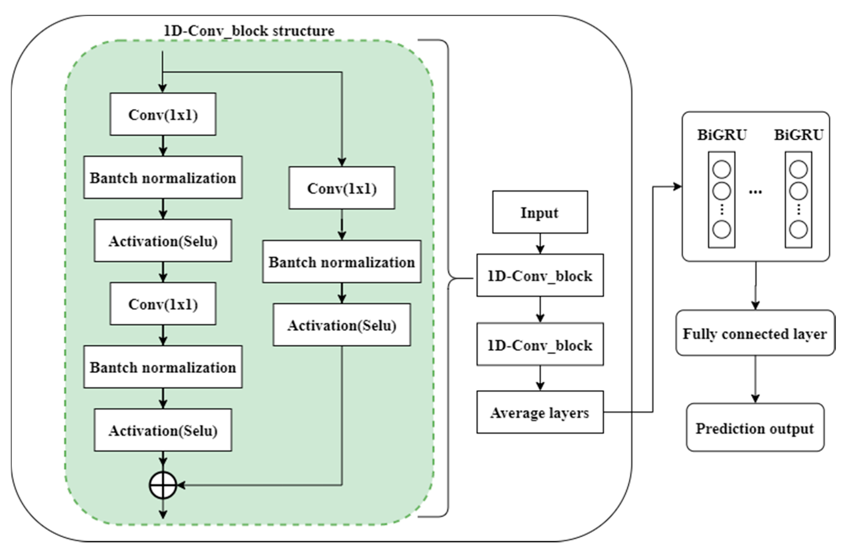
2.5. The Framework of the Proposed Model

In this paper, 1-DRCNN and BiGRU were combined to construct a hybrid neural network prediction model of water quality parameters, which consists of three parts. In the first part, the 1-DRCNN model is mainly used to mine and extract the potential nonlinear relationship features between the Luan River water quality time series data to form effective low-dimensional features. Then, the water quality feature vector is constructed from the extracted features and used as the input of the BiGRU network. The BiGRU network continuously adjusts the network weight and bias in training, and captures the dependency of short-term, long-term, and context attributes of time series data to further optimize the water quality data of feature expression. Finally, the full connection layer is connected at the top of the model as the output layer to generate the predicted values of water quality parameters. The structure of the prediction module designed in this paper is shown in Figure 4.

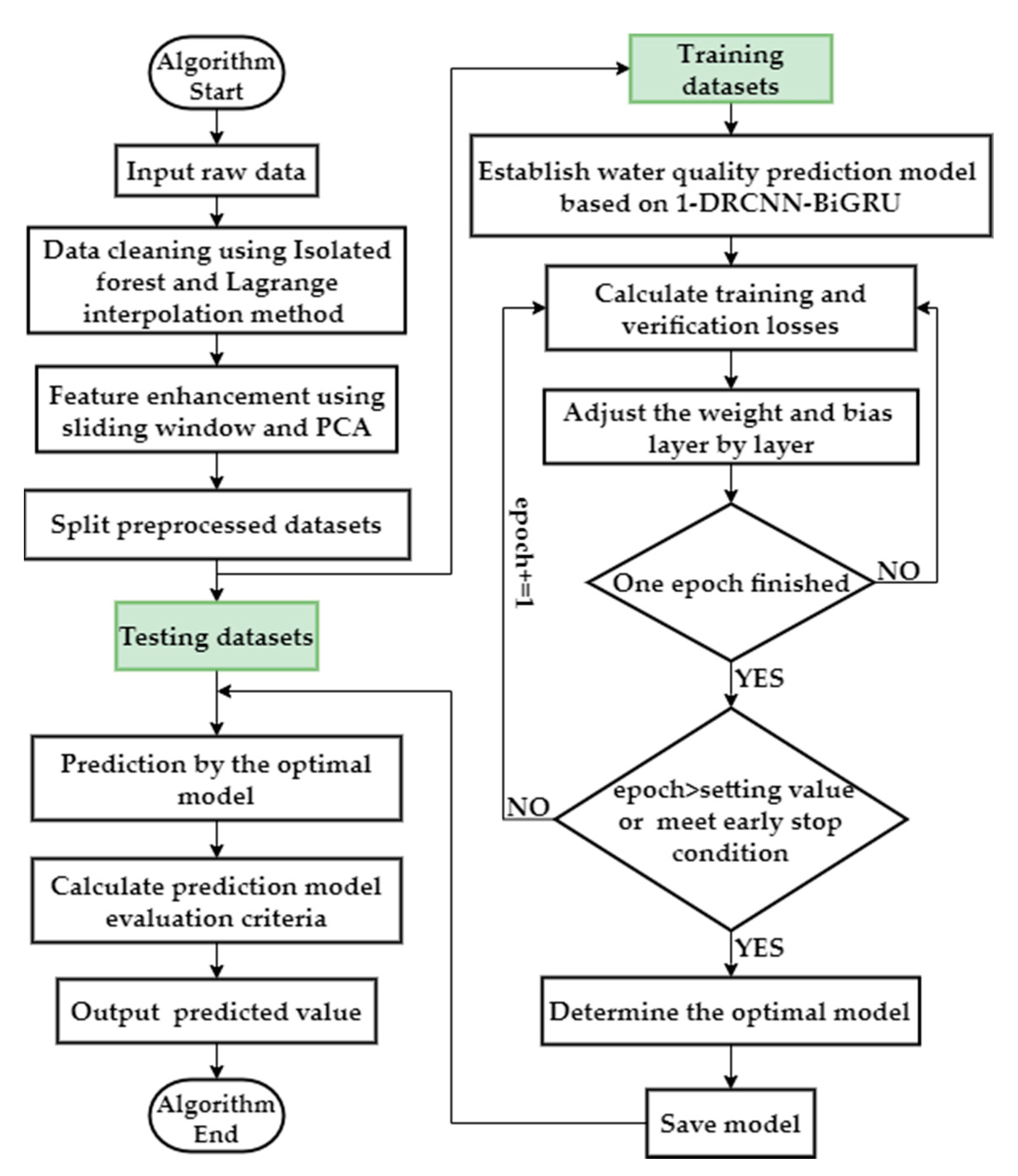
The specific process of the comprehensive water quality data prediction algorithm proposed in this paper is as follows:

Step 1: Data cleaning. Before water quality prediction, iForest in Section 2.2 is used to detect the abnormal value of water quality data ${\mathrm{X}}_{\mathrm{n}\times \mathrm{m}}$ (where n is the number of water quality parameters and m is the number of groups of data; in this paper, n and m are constant values: n = 9, m = 1360), and the abnormal value will be set to empty value. Then, Lagrange interpolation method is used to supplement the vacancy value.

Step 2: Data enhancement. Firstly, the predicted target in ${\mathrm{X}}_{\mathrm{n}\times \mathrm{m}}$ is eliminated to form ${\mathrm{X}}_{\mathrm{n}\times \left(\mathrm{m}-1\right)}$. Water quality data are collected every 4 h, and then a set of moving average ${\mathrm{Z}}_{\mathrm{n}\times \left(\mathrm{m}-1\right)}$ is generated by using the sliding window averaging technique with the window size of 6 in order to eliminate the accidental variation factors of water quality data and capture the diurnal variation trend of water quality parameters. Secondly, the principal component analysis (PCA) technology is used to reduce the dimension of ${\mathrm{X}}_{\mathrm{n}\times \left(\mathrm{m}-1\right)}$ and retain two principal components ${\mathrm{P}}_{2\times \mathrm{m}}$. To prevent the model being over-fitted, ${\mathrm{Z}}_{\mathrm{n}\times \left(\mathrm{m}-1\right)}$, ${\mathrm{P}}_{2\times \mathrm{m}}$, and water quality data ${\mathrm{X}}_{\mathrm{n}\times \left(\mathrm{m}-1\right)}$ without target parameters are concurrently taken as the input of the model, and the prediction target is used as the output of the model.

Step 3: Training model. Divide the water quality data into the training set and test set according to the ratio of 8:2. In this study, the training set contained 1088 datasets (from 5 July 2018 to 8 February 2019), and the test set contained 272 data sets (from 9 February 2019, to 26 March 2019). Because of the long-term dependence of water quality data on time, the sliding window technique [19,34] is used to divide the training set into fixed training windows with a step length of i in time sequence, and then the data of the first j training windows is used to predict the j+1th training window. For a new round of training, the oldest training window is discarded, and the next new training window is used until the last training window. By discarding the old data, one promotes the model’s learning of future trends. Then, according to the test set of each station, the trained model is used to predict the TN, TP, and COD-Mn.

The algorithm flow chart is shown in Figure 5.

2.6. Model Evaluation Criteria

To evaluate the advantages and disadvantages of the proposed prediction model and other reference methods, we used MAE, MAPE, RMSE, and ${\mathrm{R}}^2$ to evaluate the prediction accuracy of water quality parameters. The formula of each evaluation index is shown in

Table 2. Model evaluation criteria ¹.

Evaluation Criteria	Definition	Formula
MAE	Mean absolute error	$\mathrm{MAE}=\frac{1}{\mathrm{N}}{\displaystyle {\displaystyle \sum }_{\mathrm{i}=1}^{\mathrm{T}}}\left|{\mathrm{y}}_{\mathrm{i}}-{\mathrm{Y}}_{\mathrm{i}}\right|$
MAPE	Mean absolute percentage error	$\mathrm{MAPE}=\frac{1}{\mathrm{N}}{\displaystyle {\displaystyle \sum }_{\mathrm{i}=1}^{\mathrm{T}}}\frac{\left|{\mathrm{y}}_{\mathrm{i}}-{\mathrm{Y}}_{\mathrm{i}}\right|}{{\mathrm{Y}}_{\mathrm{i}}}$
RMSE	Root mean square error	$\mathrm{RMSE}=\sqrt{\frac{1}{\mathrm{N}}{\displaystyle {\displaystyle \sum }_{\mathrm{i}=1}^{\mathrm{N}}}{\left({\mathrm{y}}_{\mathrm{i}}-{\mathrm{Y}}_{\mathrm{i}}\right)}^2}$
$R^2$	Coefficient of determination	${\mathrm{R}}^2=1-\frac{{{\displaystyle \sum }}_{\mathrm{i}=1}^{\mathrm{N}}{\left({\mathrm{y}}_{\mathrm{i}}-\overline{\mathrm{Y}}\right)}^2}{{{\displaystyle \sum }}_{\mathrm{i}=1}^{\mathrm{N}}{\left({\mathrm{Y}}_{\mathrm{i}}-\overline{\mathrm{Y}}\right)}^2}$

¹ N is the size of the water quality data test sample, ${\mathrm{Y}}_{\mathrm{i}}$ is the ${\mathrm{i}}^{\mathrm{th}}$ observed value (real value) of water quality data, $\overline{\mathrm{Y}}$ is the average value of observed values of water quality data, and ${\mathrm{y}}_{\mathrm{i}}$ is the predicted value of water quality data. If the results of MAE, MAPE, and RMSE are closer to 0 and ${\mathrm{R}}^2$ is closer to 1, the prediction accuracy of the model is higher.

.

3. Results and Discussion

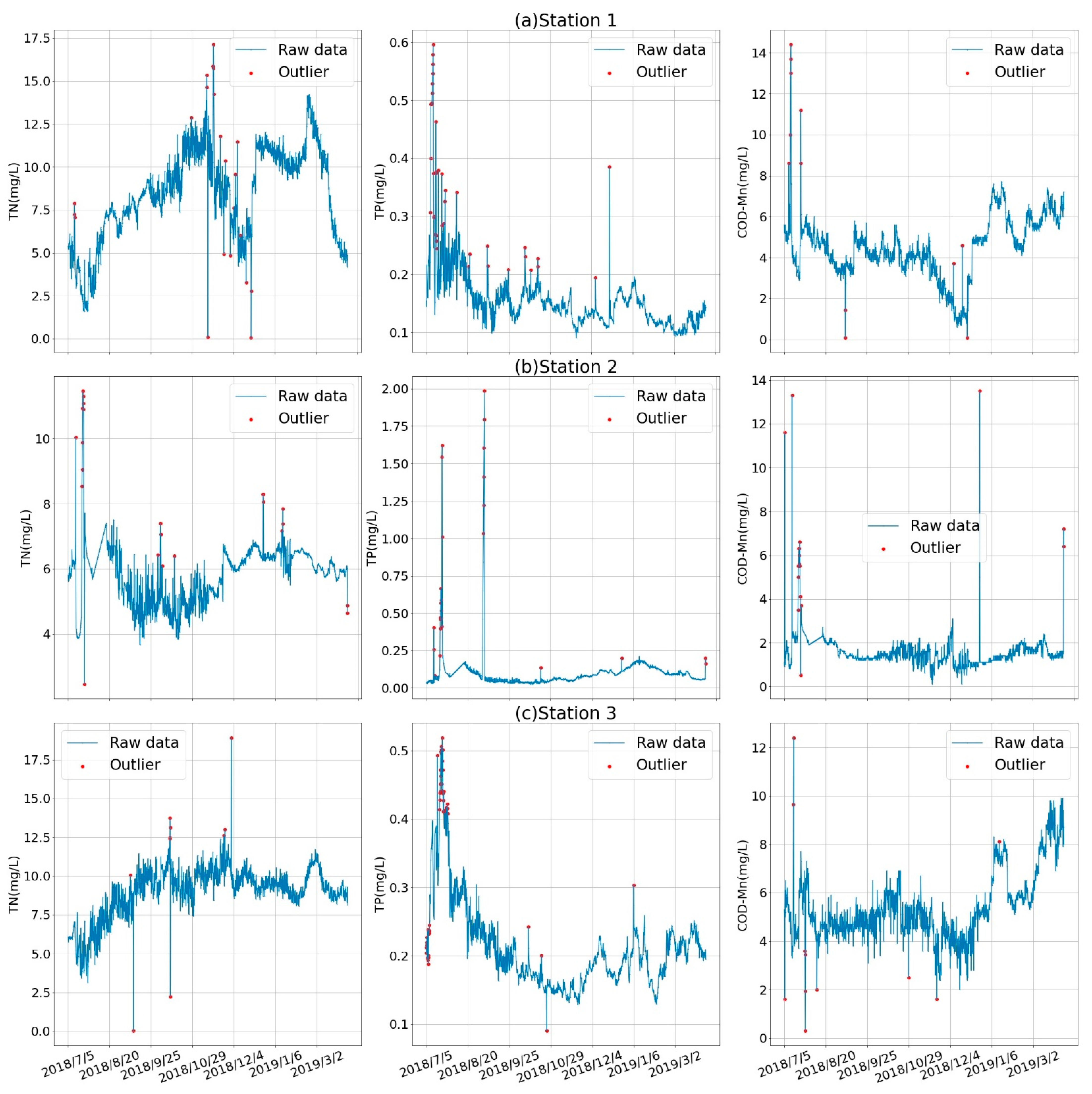
First, we used the isolation forest to detect outliers of all the water quality data of stations 1–3 in Section 2.1, accounting for about 1.1%, 1.7%, and 3.2%, respectively. Figure 6 shows the entire simulation cycle and outliers of TN, TP, and COD-Mn. After eliminating the outliers, the missing values of stations 1–3 accounted for about 3.9%, 4.5%, and 5%, respectively, and the data were corrected by the Lagrange interpolation method.

The hybrid neural network prediction model program and three reference models BiGRU, GRU, and LSTM were implemented by Tensorflows deep learning library keras2.2.0. All the models were trained in a small batch with 50 batches and 120 epochs. To prevent the overfitting of the model in the training process, we used dropout between each layer of the network, and the probability was 0.3. Adma was used as the optimizer to optimize the weight and bias of the model. Moreover, the initial training learning rate of all the models mentioned in this paper was 0.001. During model training, when the model learning stagnated, the learning rate was reduced by 10 times and the model continued to be trained. At the same time, an early training termination condition was also set. If the performance of the model did not improve significantly within 10 epochs, the training was terminated.

After a large amount of model training, the prediction effect was the best when $\mathrm{i}$ was set to 56 in the sliding window technique and $\mathrm{j}$ was set to 14. The optimal structure of the hybrid neural network model proposed in this paper was that the number of residual blocks in the 1-DRCNN model was 2, and the filter and convolution core size of the convolution layer was set to 32. The forward-propagation and back-propagation of the BiGRU module were set to two hidden layers, and the neurons in the hidden layer were respectively set to 64 and 32. To be fair, all reference models, BiGRU, GRU, and LSTM, used the same number of hidden layers and neurons. After training the model until convergence, we obtained the final weights of the 1-DRCNN-BiGRU water quality prediction model, and then the TN, TP, and COD-Mn of stations 1–3 were predicted.

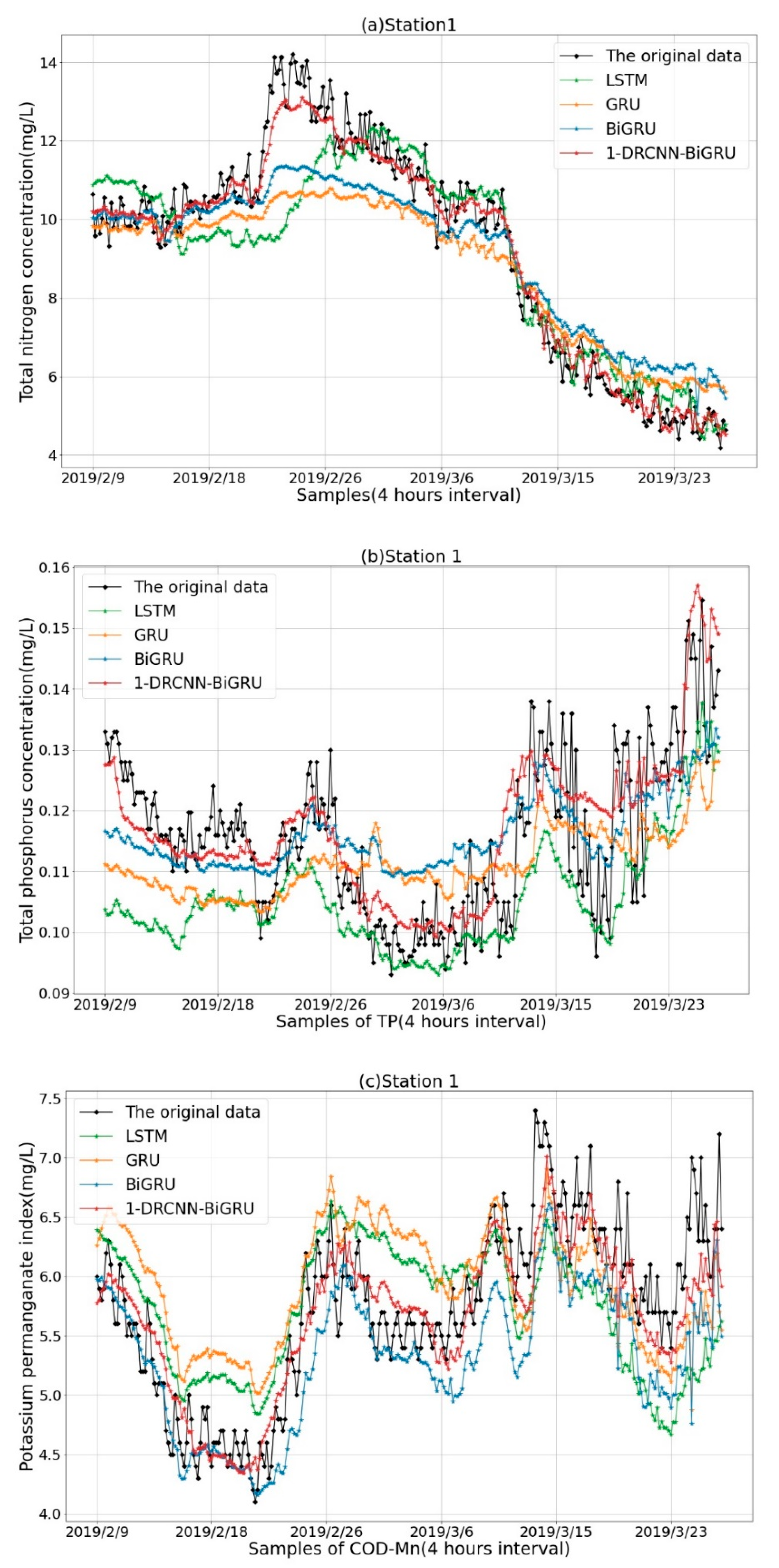
Taking TN, TP, and COD-Mn of station 1 as an example, we show the prediction results in Figure 7. It can be seen that LSTM, GRU, and BiGRU were able to roughly capture the overall trend of TN, TP, and COD-Mn. Compared with the single reference depth learning method, the 1-DRCNN-BiGRU hybrid neural network was able to more quickly and accurately capture the local change direction of these three parameters and could better follow the actual value fluctuation.

As can be seen from the model evaluation indexes of station 1 in

Table 3. Comparison between the proposed model and other models on station 1.

Water Data	Element (mg/L)	Model	MAE	MAPE (×100%)	RMSE	${\mathbf{R}}^2$
Station 1	TN	1-DRCNN–BiGRU	0.3426	3.7222	0.4531	0.9431
		BiGRU	0.8937	10.7559	1.1002	0.8416
		GRU	1.0143	11.0452	1.2709	0.7886
		LSTM	0.8436	8.7557	1.2104	0.8083
	TP	1-DRCNN–BiGRU	0.0061	4.4178	6.3964 × 10−5	0.9143
		BiGRU	0.0082	7.2932	9.6788 × 10−5	0.8321
		GRU	0.0105	8.8544	14.4888 × 10−5	0.7499
		LSTM	0.0108	8.9285	17.2758 × 10−5	0.7136
	COD-Mn	1-DRCNN–BiGRU	0.2562	5.4494	0.1070	0.9205
		BiGRU	0.4357	7.2895	0.2961	0.8361
		GRU	0.5711	10.1556	0.4127	0.7540
		LSTM	0.5770	10.3683	0.4417	0.7189

, for the parameter TN, the error metrics (MAE, MAPE, RMSE) of GRU were higher than those of LSTM, and the coefficient of determination (${\mathrm{R}}^2$) was lower than that of the LSTM model. For TP and COD-Mn, the error metrics of the GRU model were smaller than those of LSTM, and ${\mathrm{R}}^2$ was higher than that of LSTM. In this case, the prediction accuracy of GRU on TN and COD-Mn was particularly better than that of LSTM, but the opposite was true for TN. In general, although the number of internal parameters of GRU was lower than that of LSTM, the performance of predicting water quality in this study was slightly better than that of the LSTM model.

The BiGRU model performed better than LSTM and GRU models in the evaluation indexes of MAE, MAPE, RMSE, and ${\mathrm{R}}^2$ of TN, TP, and COD-Mn, indicating that the prediction performance of BiGRU for water quality parameters was improved.

For TN, TP, and COD-Mn, the method proposed in this paper had a significant improvement in the MAE, MAPE, RMSE, and ${\mathrm{R}}^2$ compared to BiGRU, especially the ${\mathrm{R}}^2$, which was stable between 0.914 and 0.944. Compared with a single model, this model had the smallest prediction error of TN, TP, and COD-Mn on station 1, and had stronger stability and robustness. Through the analysis of Figure 8 and Figure 9 and Table 3, one can conclude that the use of the 1-DRCNN–BiGRU hybrid network model is helpful in terms of improving the ability of time series feature learning and the prediction accuracy and fitting degree of water quality parameters.

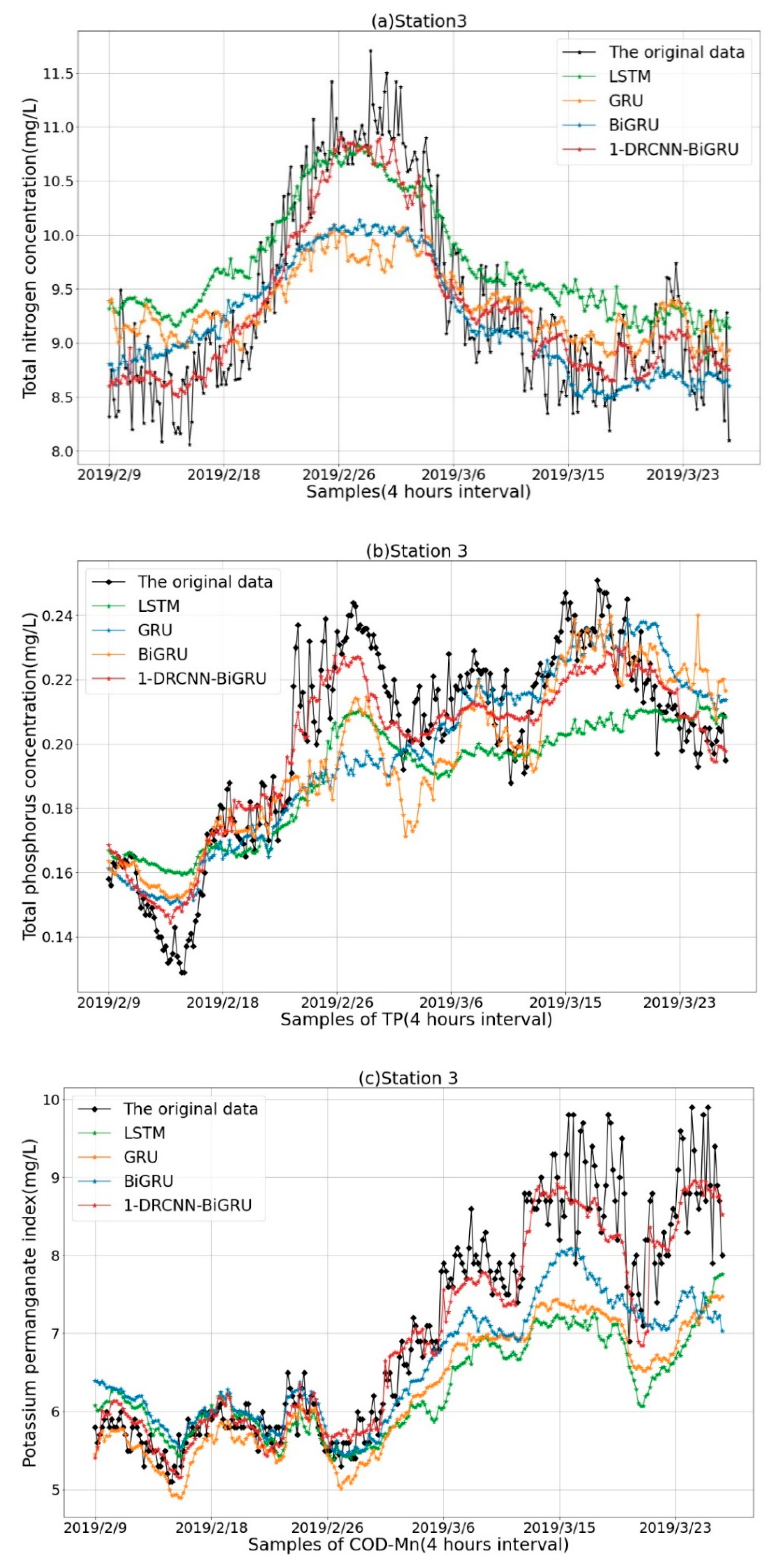
Then, the 1-DRCNN–BiGRU model trained in the above experiment was used to predict TN, TP, and COD-Mn of stations 2 and 3, and the results are shown in Figure 8 and Figure 9 and in

Table 4. Evaluation metrics of different models on stations 1 and 2.

Water Data	Element (mg/L)	Model	MAPE (×100%)	${\mathbf{R}}^2$
Station 2	TN	1-DRCNN–BiGRU	2.4866	0.9212
		BiGRU	4.6176	0.8606
		GRU	5.2087	0.7976
		LSTM	6.0147	0.7418
	TP	1-DRCNN–BiGRU	7.7839	0.9180
		BiGRU	11.8056	0.8640
		GRU	18.8431	0.8065
		LSTM	15.0313	0.7255
	COD-Mn	1-DRCNN–BiGRU	4.4659	0.9389
		BiGRU	6.7843	0.8784
		GRU	6.7242	0.7357
		LSTM	8.3243	0.7343
Station 3	TN	1-DRCNN–BiGRU	2.9738	0.9364
		BiGRU	4.4062	0.8300
		GRU	5.0924	0.7665
		LSTM	5.7688	0.7253
	TP	1-DRCNN–BiGRU	8.0103	0.9115
		BiGRU	8.3045	0.8689
		GRU	10.0388	0.8412
		LSTM	10.9675	0.7311
	COD-Mn	1-DRCNN–BiGRU	3.9316	0.9221
		BiGRU	8.2573	0.8167
		GRU	10.1405	0.7915
		LSTM	11.1497	0.7242

. It can be observed from that on stations 2 and 3, compared with the prediction results of TN and COD-Mn, the local trend of TP could sometimes not be accurately captured, but it was better than other single deep learning models. The 1-DRCNN–BiGRU model performed well on COD-Mn. Taken as a whole, by verifying on stations 2 and 3, we can conclude that the model proposed in this paper has the transferability when predicting the water quality data of different stations, which fully proves the generalization and stability of the model to predict time series water quality data.

In the article by [33], the water quality data of the Sanhedong Bridge in the Hai River Basin was used as the research object, and the PSO-DBN-LSSVR model was built to predict total nitrogen (TN). To further illustrate that the 1-DRCNN–BiGRU model used in this paper has higher prediction accuracy for time series data, we compared the TN prediction results of stations 1–3 with those in the literature [33], as shown in

Table 5. Comparison of TN prediction models.

	Element (mg/L)	Water Data	MAPE (×100%)	${\mathbf{R}}^2$
Reference [33]	TN	Reference [33]	4.32	0.9327
1-DRCNN–BiGRU		Station 1	3.7222	0.9431
		Station 2	2.4866	0.9212
		Station 3	2.9738	0.9364

. The modeling method based on 1-DRCNN and BiGRU in this paper had the smallest prediction error (the mean absolute percentage error, MAPE) and a larger coefficient of determination (${\mathrm{R}}^2$) when predicting total nitrogen, which fully demonstrates that this method performs well in predicting water quality time series and has more practical significance.

4. Conclusions

To solve the problem that the single water quality prediction algorithm cannot excavate the local characteristics of water quality and improve the prediction accuracy and efficiency, this paper proposed a data-driven water quality prediction model based on 1-DRCNN–BiGRU hybrid neural network. Firstly, the isolation forest algorithm and Lagrange interpolation methods were used to clean and correct the water quality data, which effectively improved the integrity of the data. Then, the moving average and PCA technology were used to enhance the data of water quality parameters to prevent the model from falling into overfitting. Finally, according to the preprocessed water quality data of Luan River and the sliding window technique, we constructed and verified the 1-DRCNN–BiGRU prediction model. The model organically integrates the feature extraction module and the bidirectional cycle prediction module for the first time, fully mining the local characteristics of water quality data, and was applied to the field of water quality prediction. The experimental results show that the water quality parameter prediction model has good stability and generalization ability, effectively reducing the prediction error but also providing a new idea for the prediction of one-dimensional time series data in other fields.

Although the model proposed in this paper has a good prediction advantage in the prediction of TN and COD-Mn, the prediction effect is not ideal for the dataset such as TP with a small value. Therefore, in future research, we will further consider other factors affecting water quality parameter prediction, such as transparency, chlorophyll, and heavy metals elements. At the same time, we will continue to adjust the model framework and structure, seeking a more effective network parameter optimization method and aiming to further improve the water quality parameter prediction model in smaller values of accuracy and efficiency.

References

- Li, J.F.; Zhang, J.Y.; Liu, L.Y.; Fan, Y.C.; Li, L.S.; Yang, Y.F.; Lu, Z.H.; Zhang, X.G. Annual periodicity in planktonic bacterialand archaeal community composition of eutrophic Lake Taihu. Sci. Rep. 2015, 5, 15488. [Google Scholar] [CrossRef] [PubMed] [Green Version]
- Ho, J.Y.; Afan, H.A.; El-Shafie, A.H.; Koting, S.B.; El-Shafie, A.H. Towards a time and cost effective approach to water quality index class prediction. J. Hydrol. 2019, 575, 148–165. [Google Scholar] [CrossRef]
- Zhu, L.; Li, H.; Li, J.; Dong, W. Connecting AnnAGNPS and CE-QUAL-W2 models for reservoir water quality prediction. In Proceedings of the 2011 International Conference on Electric Technology and Civil Engineering (ICETCE), Lushan, China, 22–24 April 2011; pp. 1120–1124. [Google Scholar]
- Jalowiecki, I.P.; Warrant, K.D.; Lea, R.M. WASP: A WSI associative string processor. In Proceedings of the International Conference on Wafer Scale Integration, San Francisco, CA, USA, 3–5 June 1989; pp. 83–93. [Google Scholar]
- Ei-Kaddah, D.N.; Carev, A.E. Water quality modeling of the Cahaba River. Alabama. Environ. Geol. 2004, 45, 323–338. [Google Scholar] [CrossRef]
- Zhu, C.; Liu, Q. Evaluation of Water Quality Using Grey Clustering. In Proceedings of the 2009 Second International Workshop on Knowledge Discovery and Data Mining, Moscow, Russia, 23–25 January 2009; pp. 803–805. [Google Scholar]
- Tan, G.; Yan, J.; Gao, C.; Yang, S. Prediction of water quality time series data based on least squares support vector machine. Procedia Eng. 2012, 31, 1194–1199. [Google Scholar] [CrossRef] [Green Version]
- Deng, T.; Chau, K.W.; Duan, H.F. Machine learning based marine water quality prediction for coastal hydro-environment management. J. Environ. Manag. 2021, 284, 112051. [Google Scholar] [CrossRef] [PubMed]
- Wu, G.D.; Lo, S.L. Predicting real-time coagulant dosage in water treatment by artificial neural networks and adaptive network-based fuzzy inference system. Eng. Appl. Artif. Intell. 2008, 21, 1189–1195. [Google Scholar] [CrossRef]
- Kim, S.E.; Seo, I.W. Artificial neural network ensemble modeling with conjunctive data clustering for water quality prediction in rivers. J. Hydro-Environ. Res. 2015, 9, 325–339. [Google Scholar] [CrossRef]
- Barzegar, R.; Adamowski, J.; Moghaddam, A.A. Application of wavelet-artificial intelligence hybrid models for water quality prediction: A case study in Aji-Chay river, Iran. Stoch. Environ. Res. Risk Assess. 2016, 30, 1797–1819. [Google Scholar] [CrossRef]
- Liu, S.; Xu, L.; Li, D. Multi-scale prediction of water temperature using empirical mode decomposition with back-propagation neural networks. Comput. Electr. Eng. 2016, 49, 1–8. [Google Scholar] [CrossRef]
- Long, Y.; Zhang, Y.; Wang, J.; Bai, M. Water Supply Prediction Based on Initialized Attention Residual Network. In Proceedings of the 2020 39th Chinese Control Conference (CCC), Shenyang, China, 27–29 July 2020; pp. 7367–7372. [Google Scholar]
- Zhang, Y.F.; Fitch, P.; Thorburn, P.J. Predicting the trend of dissolved oxygen based on the kPCA-RNN model. Water 2020, 12, 585. [Google Scholar] [CrossRef] [Green Version]
- Cho, K.; Merrienboer, B.V.; Gulcehre, C.; BaHdanau, D.; Bougares, F.; Schwenk, H. Learning Phrase Representations using RNN Encoder-Decoder for Statistical Machine Translation. arXiv 2014, arXiv:1406.1078v3. [Google Scholar]
- Zheng, J.X.; Chen, X.Y.; Yu, K.; Gan, L.; Wang, K. Short-term Power Load Forecasting of Residential Community Based on GRU Neural Network. In Proceedings of the International Conference on Power System Technology (POWERCON), Guangzhou, China, 24–26 October 2018; pp. 4862–4868. [Google Scholar]
- Cheng, Y.; Zhou, X.; W an, S.; Choo, K. Deep Belief Network for Meteorological Time Series Prediction in the Internet of Things. IEEE Internet Things J. 2019, 6, 4369–4376. [Google Scholar] [CrossRef]
- Zn, A.; Zy, A.; Wt, A.; Qw, A.; Mrb, C. Wind power forecasting using attention-based gated recurrent unit network. Energy 2020, 196, 117081. [Google Scholar]
- Cao, X.; Liu, Y.; W, J. Prediction of dissolved oxygen in pond culture water based on K-means clustering and gated recurrent unit neural network. Aquac. Eng. 2020, 91, 102122. [Google Scholar] [CrossRef]
- Liu, J.T.; Yu, C.; Hu, Z.H.; Zhao, Y.C. Accurate prediction scheme of water quality in smart mariculture with deep Bi-S-SRU learning network. IEEE Access 2020, 8, 24784–24798. [Google Scholar] [CrossRef]
- Tao, Q.; Liu, F.; Li, Y.; Sidorov, D. Air Pollution Forecasting Using a Deep Learning Model Based on 1D Convnets and Bidirectional GRU. IEEE Access 2019, 7, 76690–76698. [Google Scholar] [CrossRef]
- Cavalli, S.; Amoretti, M. CNN-based multivariate data analysis for bitcoin trend prediction. Appl. Soft. Comput. 2020, 101, 107065. [Google Scholar] [CrossRef]
- Shivam, K.; Tzou, J.C.; Wu, S.C. Multi-Step Short-Term Wind Speed Prediction Using a Residual Dilated Causal Convolutional Network with Nonlinear Attention. Energies. Energies 2020, 13, 1772. [Google Scholar] [CrossRef] [Green Version]
- Sun, W.T.; Su, Y.P.; Wu, X.; Wu, X.J. A novel end-to-end 1D-ResCNN model to remove artifact from EEG signals. Neurocomputing 2020, 404, 108–121. [Google Scholar] [CrossRef]
- Wang, R.; Luo, H.; Wang, Q.; Li, Z.; Huang, J. A spatial-temporal positioning algorithm using residual network and LSTM. IEEE. Trans. Inf. Meas. 2020, 69, 9251–9261. [Google Scholar] [CrossRef]
- Balanescu, M.; Suciu, G.; Badicu, A.; Birdici, A.; Zatreanu, I. Study on Unmanned Surface Vehicles used for Environmental Monitoring in Fragile Ecosystems. In Proceedings of the 2020 IEEE 26th International Symposium for Design and Technology in Electronic Packaging (SIITME), Pitesti, Romania, 21–24 October 2020. [Google Scholar]
- Cao, H.R.; Guo, Z.; Wang, S. Intelligent Wide-Area Water Quality Monitoring and Analysis System Exploiting Unmanned Surface Vehicles and Ensemble Learning. Water 2020, 12, 681. [Google Scholar] [CrossRef]
- Klambauer, G.; Unterthiner, T.; Mayr, A.; Hochreiter, S. Self-normalizing neural networks. In Proceedings of the 31st International Conference on Neural Information Processing Systems, Long Beach, CA, USA, 4–9 December 2017; pp. 972–981. [Google Scholar]
- Qin, Y.; Lou, Y.S. Hydrological Time Series Anomaly Pattern Detection based on Isolation Forest. In Proceedings of the 2019 IEEE 3rd Information Technology, Networking, Electronic and Automation Control Conference (ITNEC), Chengdu, China, 15–17 March 2019; pp. 1706–1710. [Google Scholar]
- Liu, F.T.; Ting, K.M.; Zhou, Z.H. Isolation-based anomaly detection. ACM Trans. Knowl. Discov. Data 2012, 6, 1–39. [Google Scholar] [CrossRef]
- He, K.; Zhang, X.; Ren, S.; Sun, J. Deep residual learning for image recognition. In Proceedings of the 2016 IEEE Conference on Computer Vision and Pattern Recognition (CVPR), Las Vegas, NV, USA, 10 December 2016; pp. 770–778. [Google Scholar]
- Ioffe, S.; Szegedy, C. Batch normalization: Accelerating deep network training by reducing internal covariate shift. In Proceedings of the 32nd International Conference on Machine Learning, Lille, France, 2 March 2015; pp. 448–456. [Google Scholar]
- Yan, J.Z.; Gao, Y.; Yu, Y.C.; Xu, H.X.; Xu, Z.B. A Prediction Model Based on Deep Belief Network and Least Squares SVR Applied to Cross-Section Water Quality. Water 2020, 12, 1929. [Google Scholar] [CrossRef]
- Vafaeipour, M.; Rahbari, O.; Rosen, M.A.; Fazelpour, F.; Ansarirad, P. Application of sliding window technique for prediction of wind velocity time series. Int. J. Energy Environ. Eng. 2014, 5, 1–7. [Google Scholar] [CrossRef] [Green Version]
Figure 1.
(a) Probability density distribution of TN, TP, and COD-Mn in Station 1. (b) Probability density distribution of TN, TP, and COD-Mn in Station 2. (c) Probability density distribution of TN, TP, and COD-Mn in Station 3.
Figure 2.
Residual block.
Figure 3.
(a) Basic GRU structure; (b) bidirectional GRU.
Figure 4.
The network structure of water quality prediction.
Figure 5.
Flow chart of water quality prediction algorithm based on 1-DRCNN and BiGRU.
Figure 6.
(a) The entire time series and outliers of TN, TP, and COD-Mn in station 1. (b) The entire time series and outliers of TN, TP, and COD-Mn in station 2. (c) The entire time series and outliers of TN, TP, and COD-Mn in station 3.
Figure 7.
(a) Prediction results of total nitrogen (TN) in station 1. (b) Prediction results of total phosphorus (TP) in station 1. (c) Prediction results of potassium permanganate index (COD-Mn) in station 1.
Figure 8.
(a) Prediction results of total nitrogen (TN) in station 2. (b) Prediction results of total phosphorus (TP) in station 2. (c) Prediction results of potassium permanganate index (COD-Mn) in station 2.
Figure 9.
(a) Prediction results of total nitrogen (TN) in station 3. (b) Prediction results of total phosphorus (TP) in station 3. (c) Prediction results of potassium permanganate index (COD-Mn) in station 3.