Article

Surface Characterisation of Kolk-Boils within Tidal Stream Environments Using UAV Imagery

1
Environmental Research Institute, University of the Highlands and Islands (UHI), Thurso KW14 7EE, UK
2
School of Biological Sciences, University of Aberdeen, Aberdeen AB24 2TZ, UK
3
Queen’s University Marine Laboratory, Queen’s University, Portaferry BT22 1PF, UK
4
Marine Scotland Science, Marine Laboratory, Aberdeen AB11 9DB, UK
5
Institut National des Sciences Appliquées de Lyon, 69621 Lyon, France
*
Author to whom correspondence should be addressed.
J. Mar. Sci. Eng. 2021, 9(5), 484; https://doi.org/10.3390/jmse9050484
Submission received: 30 March 2021 / Revised: 19 April 2021 / Accepted: 29 April 2021 / Published: 30 April 2021
(This article belongs to the Section Ocean Engineering)

Abstract

:
High-flow tidal stream environments, targeted for tidal turbine installations, exhibit turbulent features, at fine spatio-temporal scales (metres and seconds), created by site-specific topography and bathymetry. Bed-derived turbulent features (kolk-boils) are thought to have detrimental effects on tidal turbines. Characterisation of kolk-boils is therefore essential to inform turbine reliability, control, and maintenance strategies. It will also improve the understanding of potential ecological interactions with turbines, as marine animals use these sites for foraging. Unmanned aerial vehicle (UAV), or drone, imagery offers a novel approach to take precise measurements of kolk-boil characteristics (distribution, presence, and area) at the surface. This study carried out sixty-three UAV surveys within the Inner Sound of the Pentland Firth, Scotland, UK, over four-day periods in 2016 and 2018. Kolk-boil characteristics were examined against relevant environmental covariates to investigate potential drivers of presence and area. The results show that distribution at the surface could be predicted based on tidal phase, with current velocity significantly influencing presence above 3.0 m/s. The technique can be used to inform turbine development, micro-siting and provide better understanding of environmental implications of turbine operation. Finally, it highlights the suitability of UAVs for capturing rapid fine-scale hydrodynamic data in the absence of in situ measurements.

1. Introduction

With global concern over the impacts of climate change, the 2015 Paris Agreement necessitating net-zero carbon emission energy systems by 2100, and many countries committing to achieving this by 2050, there is an increasing demand to use renewable energy sources [1,2,3]. Marine renewable energy (MRE) resources have been estimated to exceed both present and projected global demands, and are an area currently experiencing a wealth of research and development [4]. A key sector of the industry is tidal stream energy extraction (hereafter tidal energy), which offers a predictable, renewable, energy source with a worldwide projected extractable capacity in excess of 120 GW [5,6].
Tidal stream environments are coastal habitats characterised by tidal forcing of large volumes of water through restrictive channels, or around headlands and islands, creating fast flowing waters in excess of 1 m/s [7]. Tidal forcing causes the formation of bed-derived turbulent flow structures, such as kolks, bursts and kolk-boils, created by the water interacting with the bathymetry [8]. It also generates coastally-derived features (eddies and wakes), as a result of the differences in velocities at boundaries, as well as open-water features (tidal jets) triggered by pressure changes from water height differences [8].
There is a growing awareness that turbulent features occurring at fine spatio-temporal scales (metres and seconds) have detrimental effects on tidal turbine power output, reliability and efficiency [9]. It is therefore clear that an understanding of turbulent features should inform turbine design and micro-siting in order to more accurately calculate the loading on each device, the rate of fatigue on material components and the range of fluctuations in power output that may be experienced [10,11]. These turbulent features are also important in determining animal presence within tidal stream environments, as they offer potential foraging hotspots for mobile predators (seabirds and mammals) because of the influence of flow variation on the distribution of prey species (fish) [8,12,13]. Therefore, to comprehend the full environmental and ecological impact of tidal energy developments, which can be a barrier to successful consenting and licensing of MRE devices and arrays, fine-scale hydrodynamic habitat characterisation is required by current and future projects [12].
While current velocity is relatively simple to measure in tidal stream environments, quantification and characterisation of ephemeral bed-derived turbulent features, such as kolk-boils, is still lacking [9]. Kolk-boils, bursts or boils (collectively referred to as kolk-boils hereafter) are turbulent features that can be observed at the surface as a smooth patch of water surrounded by a heavily contrasting perimeter of dissipating waves or bubbles [14]. When fast flowing water hits a significant bathymetric feature, usually the rear side of the crest of a ridge or dune known as the “separation zone”, the water is slowed and begins to rotate forming a hairpin vortex (hereafter referred to as a kolk) (Figure 1) [15]. This rotating water mass separates from the main flow and the seabed, moving down the lee of the feature to collate in the nearest trough, called the “reattachment zone” (Figure 1) [16].
The kolk is then advected by the following incline and moves upward through the water column, while still being pushed horizontally by the prevailing current direction, until its head meets the surface (Figure 2) [17]. When this converging event occurs, it causes an initial eruption of fluid in the form of steep outward-moving surface waves which quickly dissipate due to being at the extent of their energetic reach [18]. This dissipation appears as a patch of smooth upwelling which swiftly forms a circular, or elliptical, pattern as more fluid rises from the kolk and moves outward from the initial point of eruption [19].
Figure 2. A schematic detailing kolk-boil formation at the sea surface [20].
Jmse 09 00484 g002
Empirical measurement of turbulence within the marine environment has conventionally used acoustic Doppler current profiling (ADCP) devices measuring at one, or in an array of, locations upward throughout the water column [21,22]. While this approach can assess flow characteristics, and thus predict turbine energy yield, it does not have the necessary spatial resolution to accurately capture fine-scale coherent turbulent structures such as kolk-boils [21]. Additionally, tidal stream environments are challenging to survey due to strong tidal flows and inherent turbulence, adding extra logistical, financial and risk considerations to any in situ data collection effort [12,23]. Hence, there is an urgent need for suitable platforms that can safely, and cost-effectively, survey tidal stream environments at the fine-scale spatio-temporal resolutions required [24]. Investigations into remote sensing techniques, as a means to remedy this, have highlighted the viability of quantifiable measurements through imagery of the surface [22,25].
This study used unmanned aerial vehicles (UAVs), launched from a moving ship during four days of continuous surveys in both 2016 and 2018. The aim was to characterise the spatial distribution of kolk-boils within a tidal stream environment, and then relate key physical environmental properties (current velocity, current direction, tidal phase, depth, seabed roughness, slope angle and aspect) to boil presence and area at the surface to understand the drivers and predictability of these features.

2. Materials and Methods
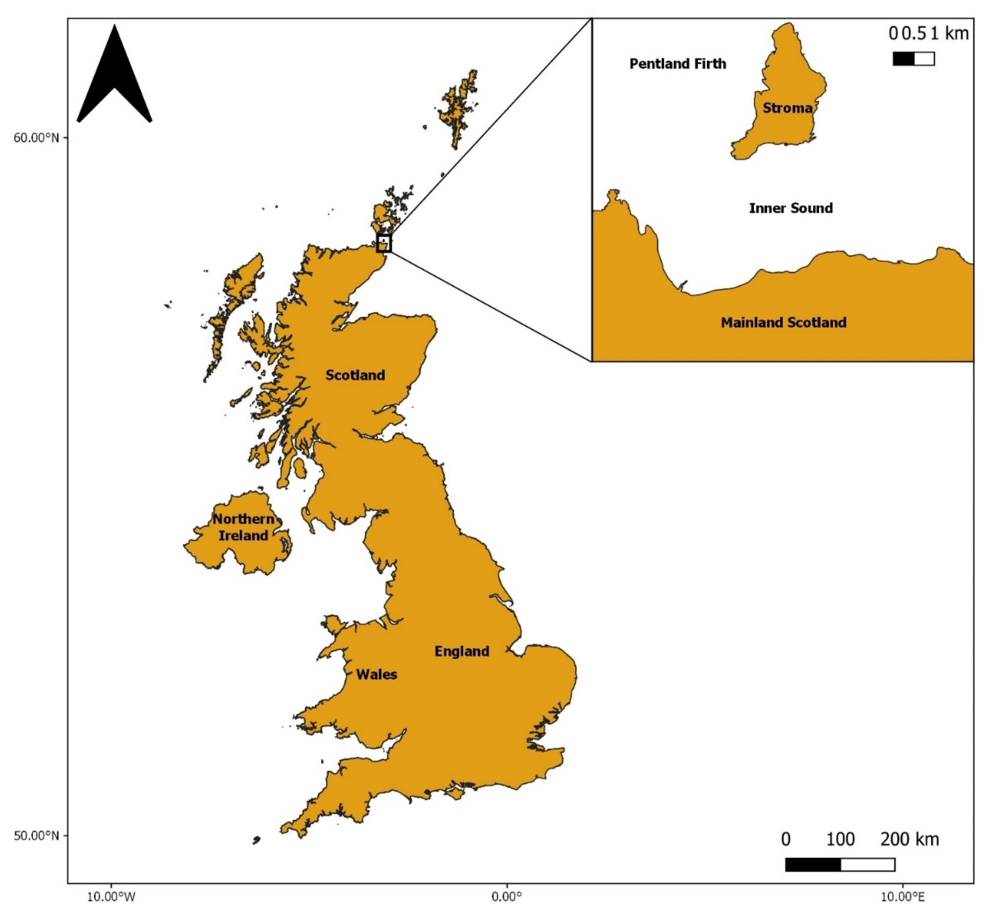
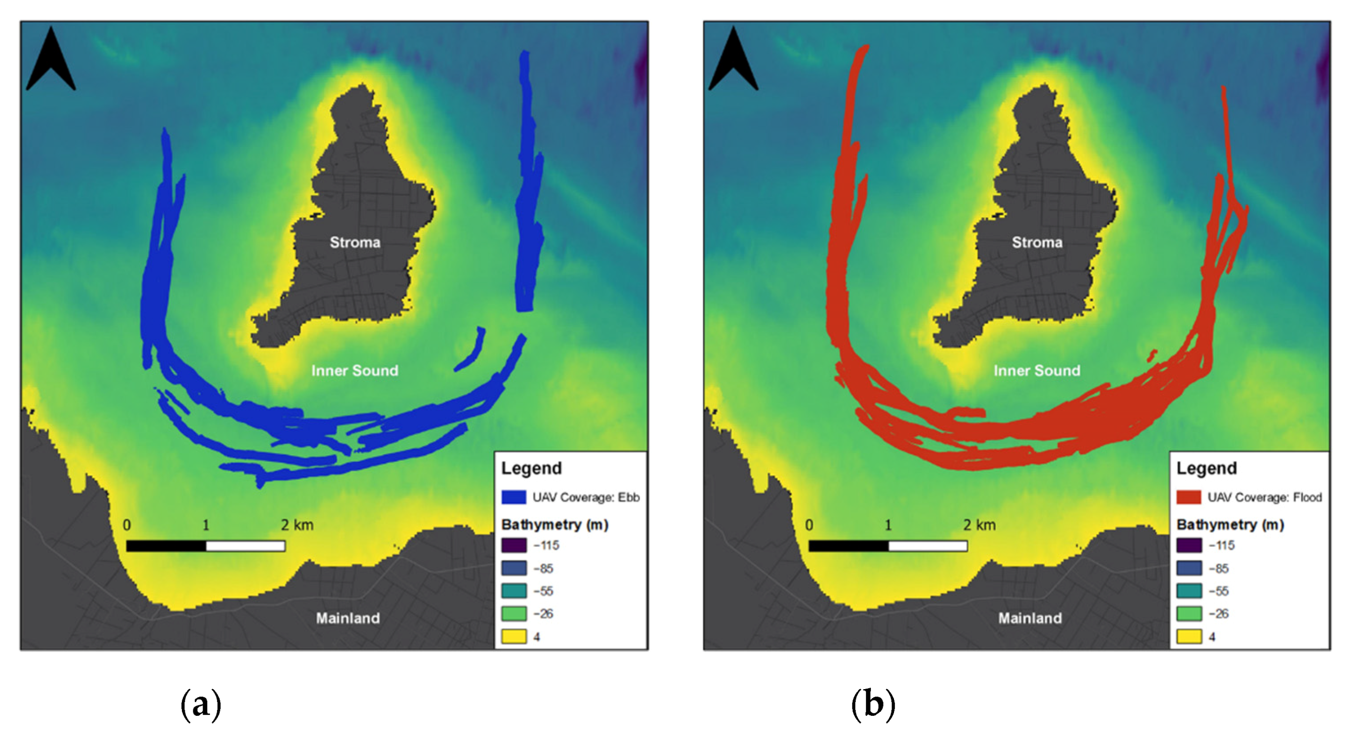
2.1. Study Site

Measurements were carried out in the Pentland Firth, UK, an active tidal stream energy lease site. The Pentland Firth is a 20-km long channel of water that separates mainland Scotland from the Orkney Islands and connects the North Atlantic Ocean to the North Sea [26,27] (Figure 3). Due to a large variance in tidal phase, when moving from either entrance of the channel, and topographic restrictions recorded current velocities regularly exceed 2 m/s [26,28,29]. As part of the Pentland Firth, the Inner Sound is a contributory channel of water between the Scottish mainland and the Island of Stroma with an average maximum depth of 35 m (Figure 3) [30]. During flood spring tides, current speeds within the Inner Sound have been recorded up to 6 m/s, with a predicted energy potential of approximately 1.9 GW [28]. This makes it one of the most prominent tidal lease sites within the UK and is home to the MeyGen project, operated by SIMEC Atlantis Energy (SIMEC), which has a total planned capacity of 398 MW [31,32,33]. Since 2016, SIMEC have installed four 1.5 MW turbines that have surpassed 23 GWh in total energy generation, as of December 2019, transmitting an estimated 800 MWh energy to the grid per month [32,33,34]. Surveys were conducted prior to turbine installation (2016) and once the turbines were installed (2018). The study focuses on kolk-boil characterisation rather than any turbine-derived hydrodynamic effects.

2.2. Data Collection

Twenty-five UAV surveys were conducted between 23 and 25 June 2016 and thirty-eight between 21 and 24 July 2018 from a moving vessel (MRV Scotia) transiting continuously around the Island of Stroma. A multirotor UAV was used in both instances due to the capability to hover, meaning increased stability and positional control and thus higher accuracy for fine-scale survey work such as this [35]. UAV surveys were focused on the Inner Sound with flights occurring near-continuously, weather permitting, during daylight hours and across differing phases of the tidal cycle (ebb/flood) (Figure 4). This culminated in 15 h and 13 min of total flight time. All flights were undertaken according to Civil Aviation Authority regulations for UAV operation, as well as adhering to recommended best practice guidelines for UAV usage within environmental research [36,37].
UAV take-off occurred from a consistent location on the deck of the MRV Scotia of a known height above sea level (10.6 m). During operation, all surveys were manually flown at a consistent speed over ground. This was kept consistent by monitoring onboard GPS speed readouts. Flights were carried out at windspeeds <5 m/s for safety, which was well within the capability specified by the UAV manufacturer [38]. All flights were conducted against the prevailing current direction to avoid miscounting objects of interest. Flight durations ranged between 10 and 30 min, with an average of over 200 JPEG images taken during each survey. While the overall methodology remained the same across both years, with comparable ground sampling distances, upgrades were made to camera and UAV specifications moving from 2016 to 2018 (Table 1). Although relative altitude, and area of each image, varied between years, altering overall coverage, processes described within Section 2.3 meant that this had no impact on the accuracy of detection and measurements taken during data processing.

2.3. Data Processing

Images were registered in space and time using onboard telemetry data, in this case altitude, heading and the coordinates (of the central point) of each image. In combination with the calculation of camera specific calibration values, using an equation detailed in Appendix A (Equation (A1)), this allowed for the orthorectification of the image calibrating units from pixels to metres. This then permitted calculation of latitude and longitude values for objects of interest and the plotting of physical coverage over ground.
Images were examined manually, without the aid of automated techniques, to detect and parameterise kolk-boils within them. This was performed using a graphical user interface (GUI) which was developed within MATLAB (R2019b; MathWorks) to process and collate the multiple images taken within each survey. The GUI’s main functions were to allow a user to track kolk-boils between images (avoiding misidentification and overestimation of targets), to manipulate individual images, log information such as kolk-boil location (central point), number, classification (type, confidence and if it was present on the previous image) and measurements of the perimeter (for fully formed features), and finally provide relevant image and telemetry information. The GUI allowed the user to sequentially move through all the images in a selected survey and record an unlimited number of kolk-boils within each image.
User observation time (effort) for each image was dependent on the number of potential kolk-boils detected. Due to the targets being sizable features (>100 m2 (Figure A1), i.e., >15% of an image) it was possible to quickly identify if no kolk-boils were present and the user could move to the next image if that was the case. If the same kolk-boil was present across multiple images, it was noted what number (identifier) that boil had in the previous image and was recorded as part of the classification process. Once started, a survey was processed in one operation, by the same user, to maintain consistency and avoid between-user bias.
For the purposes of this study, a kolk-boil was classified as a “glassy” or “smooth” circular/elliptical patch of water, with a definitive perimeter, that was visibly different from the surrounding water [14]. The perimeter was defined as the outermost edge of the rough waves or bubbles, which comprise a kolk-boil’s boundary, that could be seen to meet with the general body of water present within the image (Figure 5) [39]. This was stipulated to increase the accuracy of area measurements taken and to maintain consistency throughout the user’s inputs. Kolk-boils were split into four types consisting of formed (the perimeter of waves or bubbles visually appears ≥70% complete), un-formed (the perimeter of waves or bubbles visually appears <70% complete), unknown (kolk-boil is partially present on the image, thus determining if it is formed or un-formed is not possible) and other (a turbulent feature that is not a kolk-boil such as an eddy or wake) (Figure 5). These classifications allowed the user to quantify boil presence and area during post-processing. For area, a measurement of the perimeter of a feature was required. For presence, a boil (formed, un-formed or unknown) only needed to be detected within an image. With limited recommendations from the relevant literature, these classifications were estimated visually by the user. A confidence score (out of 100) was given to each boil. This was based on visible quality and how distinct the feature was from the background. This corresponded to high (≥80), good (50–70) and poor (≤40) quality. The criterion was also applied visually, by the same user, to minimise inconsistencies and subjectivity.

2.4. Post-Processing

This study characterised kolk-boils based on distribution, presence, and area at the surface. Distribution was based on the central point of formed kolk-boils and was examined against tidal phase and current velocity to investigate spatial patterns. Boil presence (using formed and un-formed boils) and area (using formed boils) were then examined in relation to environmental covariates. Boil presence was categorised as an image with a boil detected within it, while absence was classed as an image with no boil detected within. Finally, boil area was calculated from perimeter measurements taken of formed boils.
An output file was collated for each survey, with these being merged into a single dataset. This included kolk-boil central point position, kolk-boil area (m2), kolk-boil classification (type and confidence), kolk-boil presence, telemetry data, and relevant explanatory variables taken from the central point of each image (current velocity (m/s), current direction (degrees), tidal phase (assigned based on the average current velocity and direction), depth (m), seabed roughness (m), slope angle (degrees) and aspect (degrees)). Kolk-boils deemed to be visually poorly defined (≤40 confidence score) were excluded due to significant uncertainty around whether they were kolk-boils.
Hydrodynamic variables (current velocity, current direction, and tidal phase) were obtained from a depth-averaged TELEMAC-2D model output for the location and timestamp of each image. The hydrodynamic model was constructed using the non-hydrostatic version of the programme which solves the Saint-Venant equations. The K-epsilon turbulence closure model was used. Two-dimensional model grid resolution varied from 50 m within 2 km of the Island of Stroma, 200 m within 1 km of other coastlines, 500 m resolution at open water boundaries, and 1 km resolution elsewhere. For a desired Courant number close to 1, a time step of 30 s was selected based on flow rates in the vicinity [40]. While individual current velocity and current direction values were taken directly from the hydrodynamic model for each image, tidal phase categorisation was assigned from the average current velocity and current direction across each survey. This was split into six factors: fast ebb (<−1 m/s), decreasing ebb (−1 to −0.26 m/s), increasing ebb (−0.26 to −1 m/s), fast flood (>1 m/s), decreasing flood (1 to 0.26 m/s) and increasing flood (0.26 to 1 m/s) as used in Zamon et al. [41] when quantifying tidal phase within a tidal stream environment.
A 0.20 m resolution bathymetry raster, from multibeam survey data (MeyGen Ltd., Edinburgh, UK), was used to calculate depth, seabed slope angle, roughness, and slope aspect values from the central point of each image. This was achieved using the “Point Sampling Tool” and “GDAL Tools” plugins within QGIS (QGIS Development Team, 2020). While depth, seabed slope angle and aspect values were taken directly from the bathymetry data as point values, roughness (the degree of irregularity of the seabed in metres) involved the calculation of the largest inter-cell difference between the central image point value and those immediately surrounding it [42].

2.5. Data Analysis

A Generalised Additive Model (GAM) was used to analyse the suite of explanatory variables potentially influencing the probability (p) of kolk-boil presence, at the surface, within the Inner Sound (using the mgcv package in R [43]). The kolk-boil presence GAM (n = 7236) assumed a Bernoulli distribution with logit link and included smoothing functions for all non-parametric variables. The maximum variation of each smoothing function was specified via the number of knots (k) provided to each spline and tensor product. This was initially set to five (or five by five for tensor products) for each variable, as there was only minor variation (i.e., some non-linearity which could be suitably estimated using only five knots). It was subsequently checked if the number of knots were sufficient by using the k-index and approximate p-values in ‘mgcv::gam.check()’. Knots were increased, as required, until the k-index approached one, and the approximate p-values were not significant. Thin plate regression splines (f1, f3, f4 and f6) were used for current velocity (k = 8), seabed slope angle (k = 5), depth (k = 5) and seabed roughness (k = 5). Cyclic cubic regression splines (f2 and f5) were applied when modelling seabed slope aspect (k = 5) and current direction (k = 5) as for both variables 0° must match 360°. Two anisotropic tensor products (f7 to f8), henceforth referred to as “interaction” included current velocity and seabed slope angle (k = 5 and 5), as well as current direction and seabed slope aspect (k = 5 and 5) in the model. The first interaction used thin plate splines for both variables while the second utilised cyclic cubic regression splines. The model included tidal phase (α0 to α4) as the only parametric variable. This included declining ebb (DE), declining flood (DF), fast ebb (FE), fast flood (FF) and increasing flood (IF) phases. To avoid the issue of complete separation, and the Hauck–Donner effect, within the binomial model the increasing ebb phase (IE) data, due to having minimal effect on the overall model fit, were removed from analysis. The numeric classification given to each individual flight ϛ(FlightIDi) was incorporated into the final model as a random effect variable to account for temporal autocorrelation.
Presence ~ Bernoulli(pi)
logit(pi) = α0TidalPhaseDE,i + α1TidalPhaseDF,i + α2TidalPhaseFE,i + α3TidalPhaseFF,i + α4TidalPhaseIF,i + f1(Current Velocityi) + f2(Seabed Slope Anglei) + f3(Depthi) + f4(Seabed Roughnessi) + f5(Current Directioni) + f6(Seabed Slope Aspecti) + f7(Current Velocityi, Seabed Slope Anglei) + f8(Current Directioni,Seabed Slope Aspecti) + ϛ(FlightIDi)
Restricted maximum likelihood (REML) was used for parameter estimation [44]. Model assumptions and the complexity of the fitted smooth function were checked and deemed to be met (Figure A3, Figure A4 and Figure A5). An additional penalty term was applied for smoothness selection (via the mgcv argument, select = TRUE). This automatically shrinks non-influential variables by heavily penalising them, thus removing them from the model [45]. To check if the only parametric parameter, tidal cycle, was influential and should be included in the final model, the Akaike information criterion (AIC) was used to compare models with, and without, tidal phase.
While measurements of the area of formed boils were recorded and compared against the same variables as presence (Figure A1), analysis highlighted the need for a larger data set to draw any meaningful conclusions on the potential environmental influences of kolk-boil area at the surface (Figure A2, Figure A6, Figure A7 and Figure A8). Area of boil was therefore removed from further analysis at this point but was retained within the Appendix A. This was done to highlight the ability to quantify this variable from UAV imagery and its potential relevance in future work.

3. Results

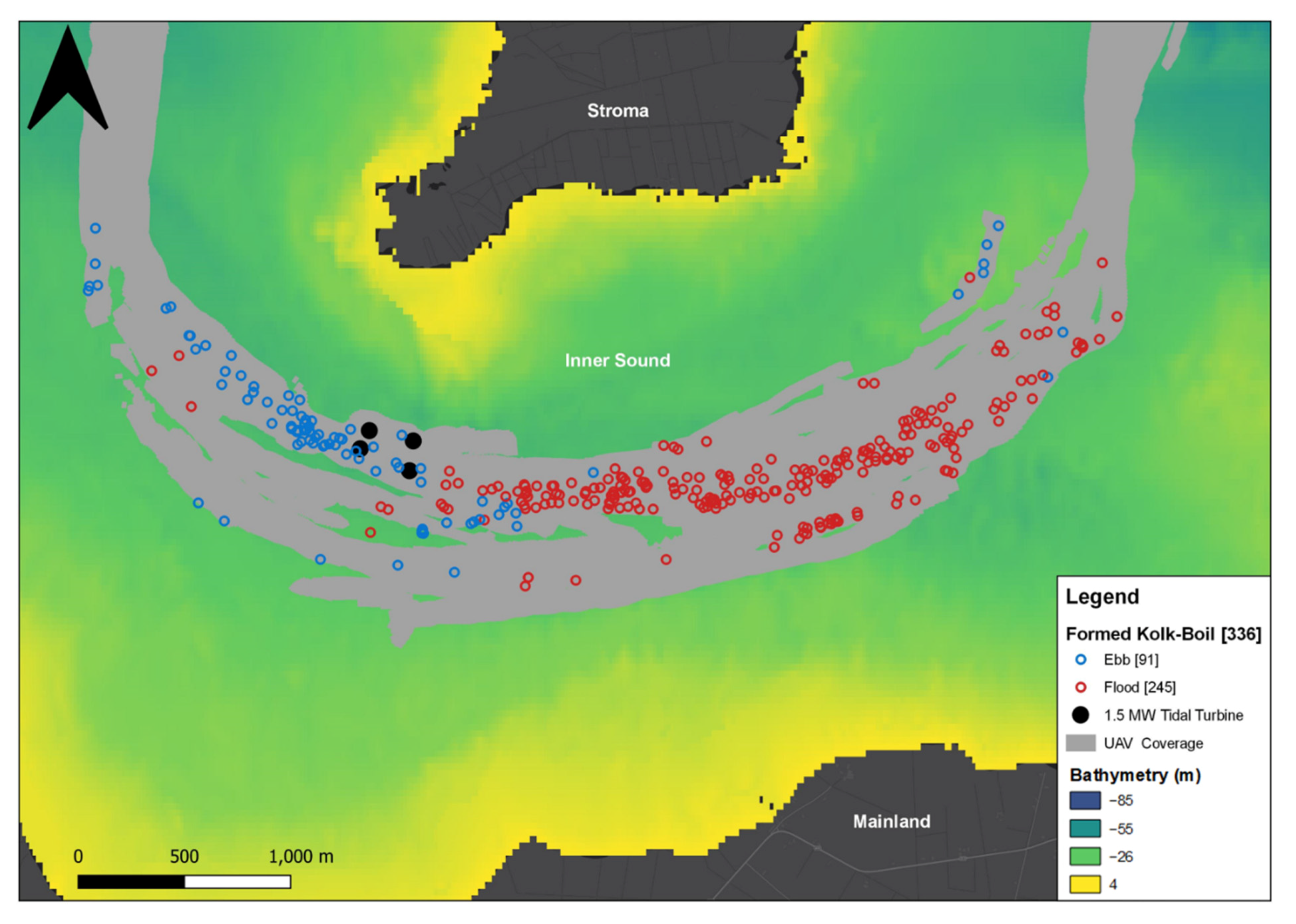
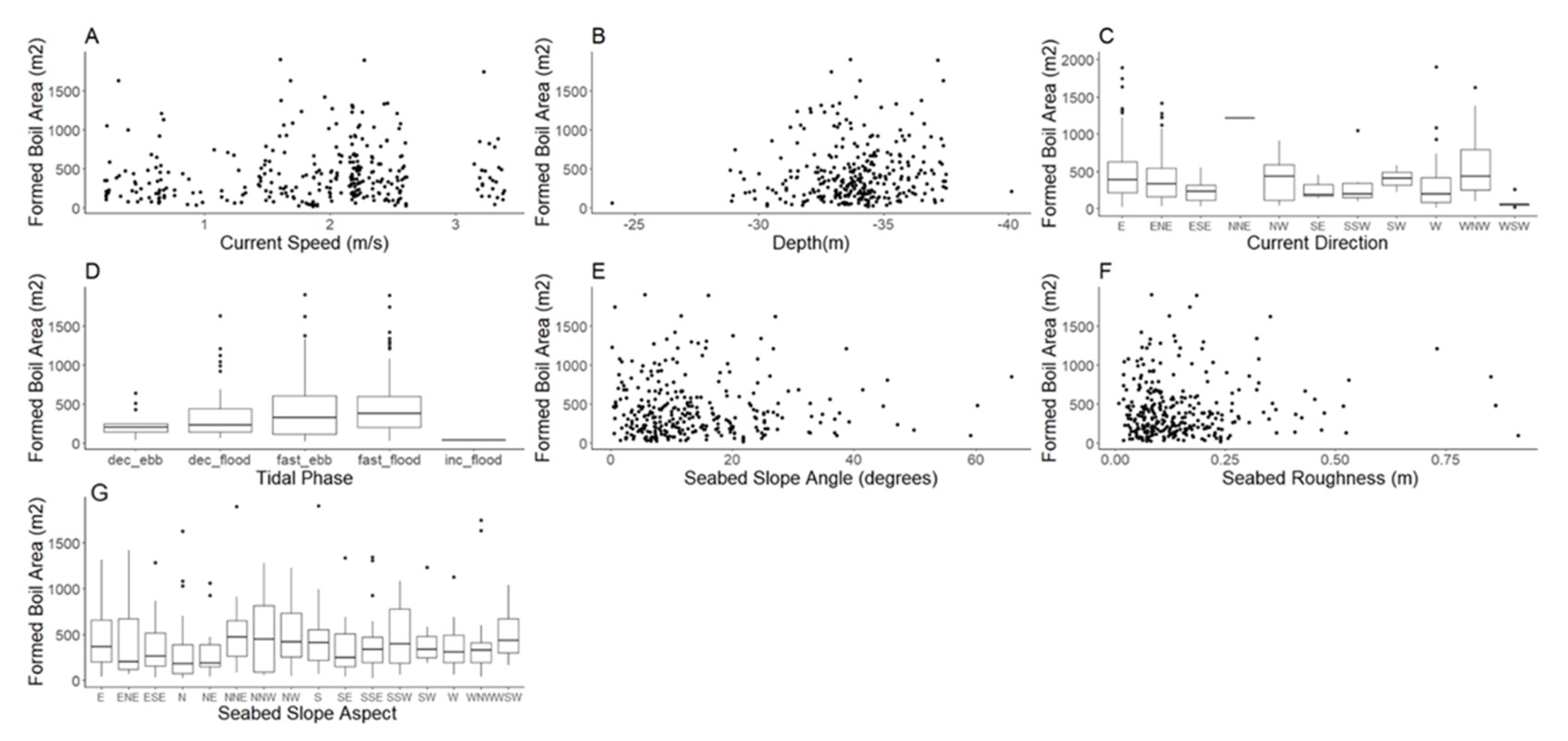
3.1. Kolk-Boil Distribution

A total of 336 formed kolk-boils were present within much of the surveyed area of the Inner Sound (Figure 6). Spatial clustering of kolk-boils was apparent within the centre of the channel, as well as a clear asymmetry being observed when the distribution of these features was examined based on tidal phase (Figure 6). Formed kolk-boils detected on the ebb phase (27.1% of all kolk-boils) were predominantly observed at the western side of the Inner Sound, while those detected on the flood phase (72.9% of all kolk-boils) were found in the central and eastern areas of the channel.

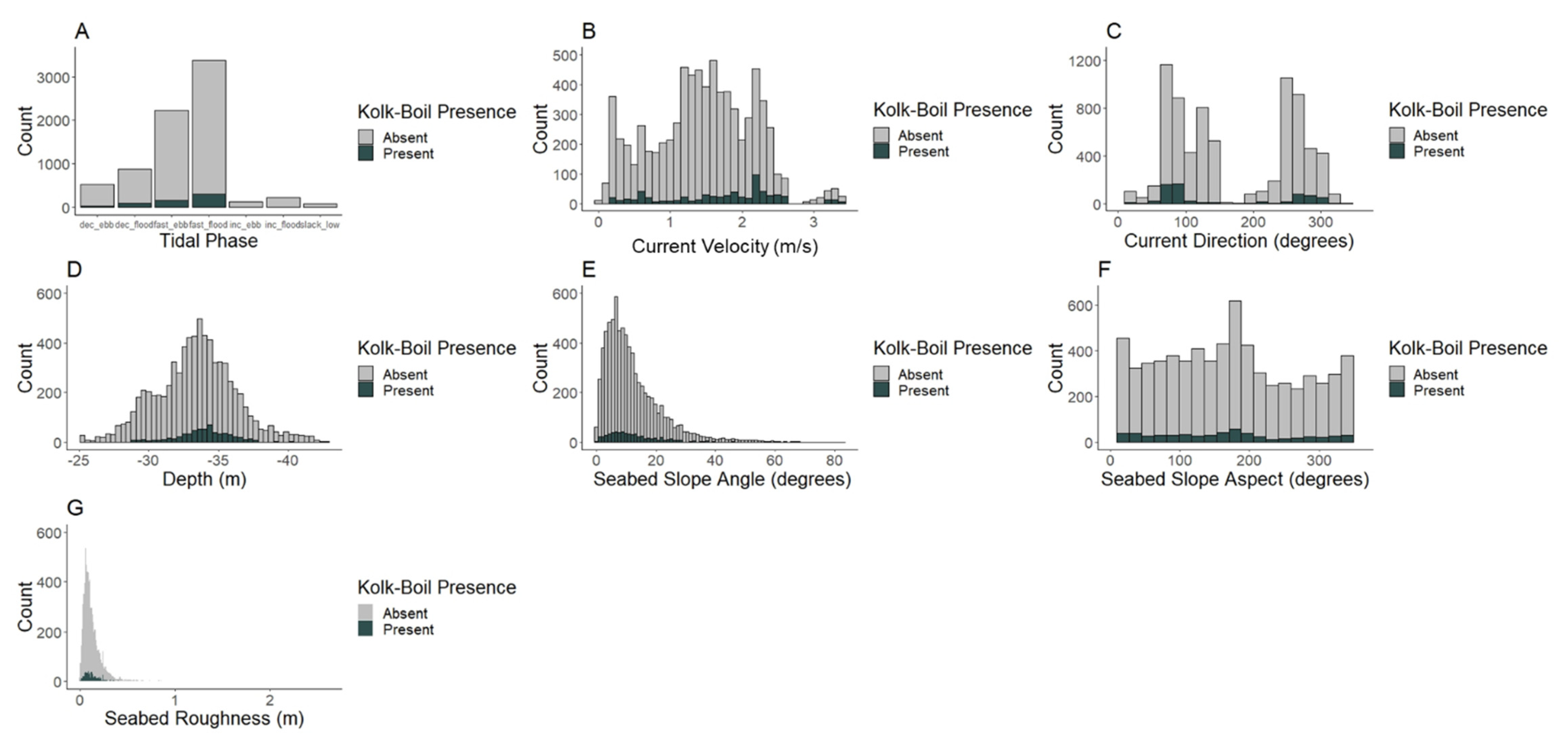
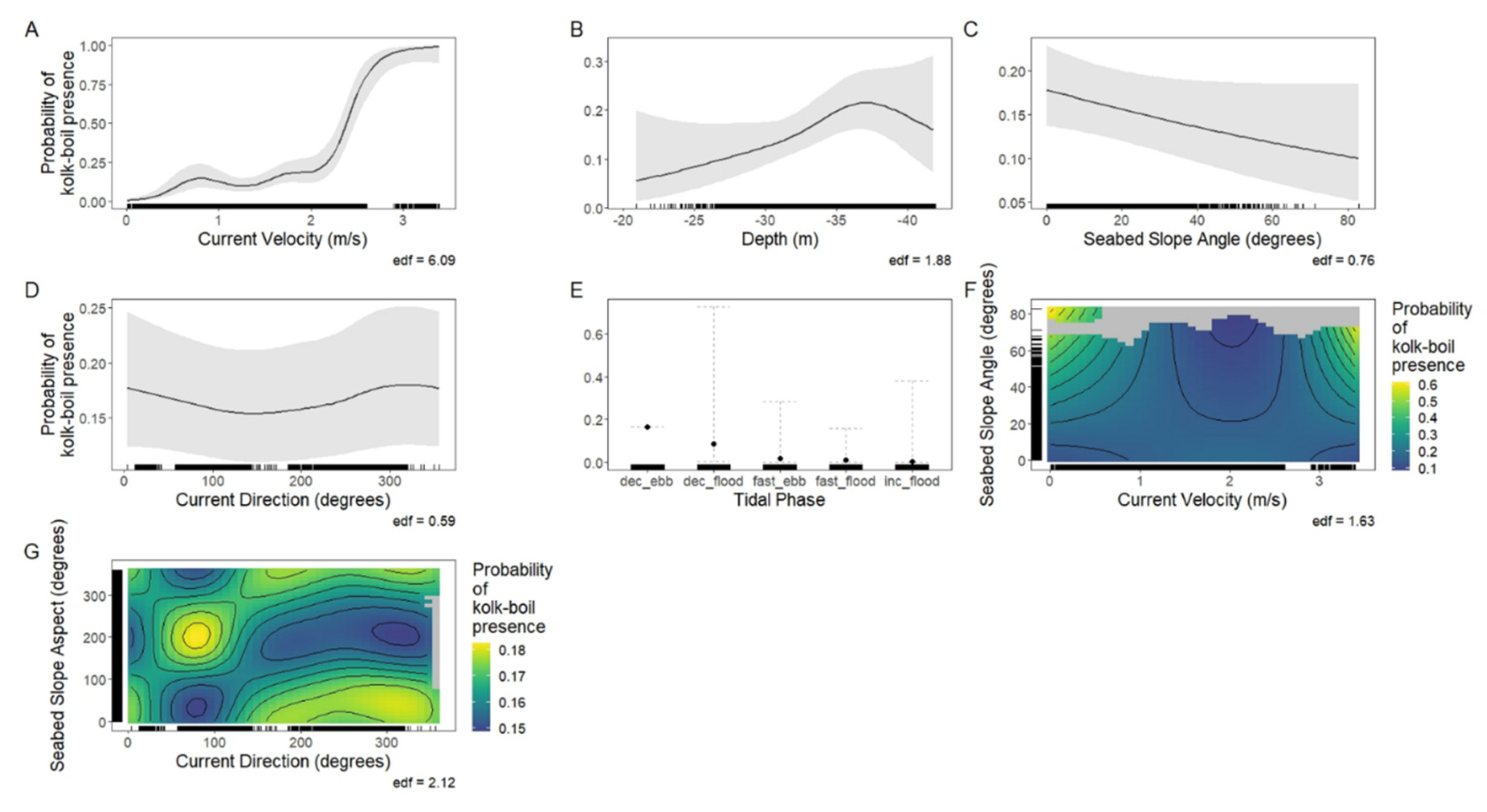
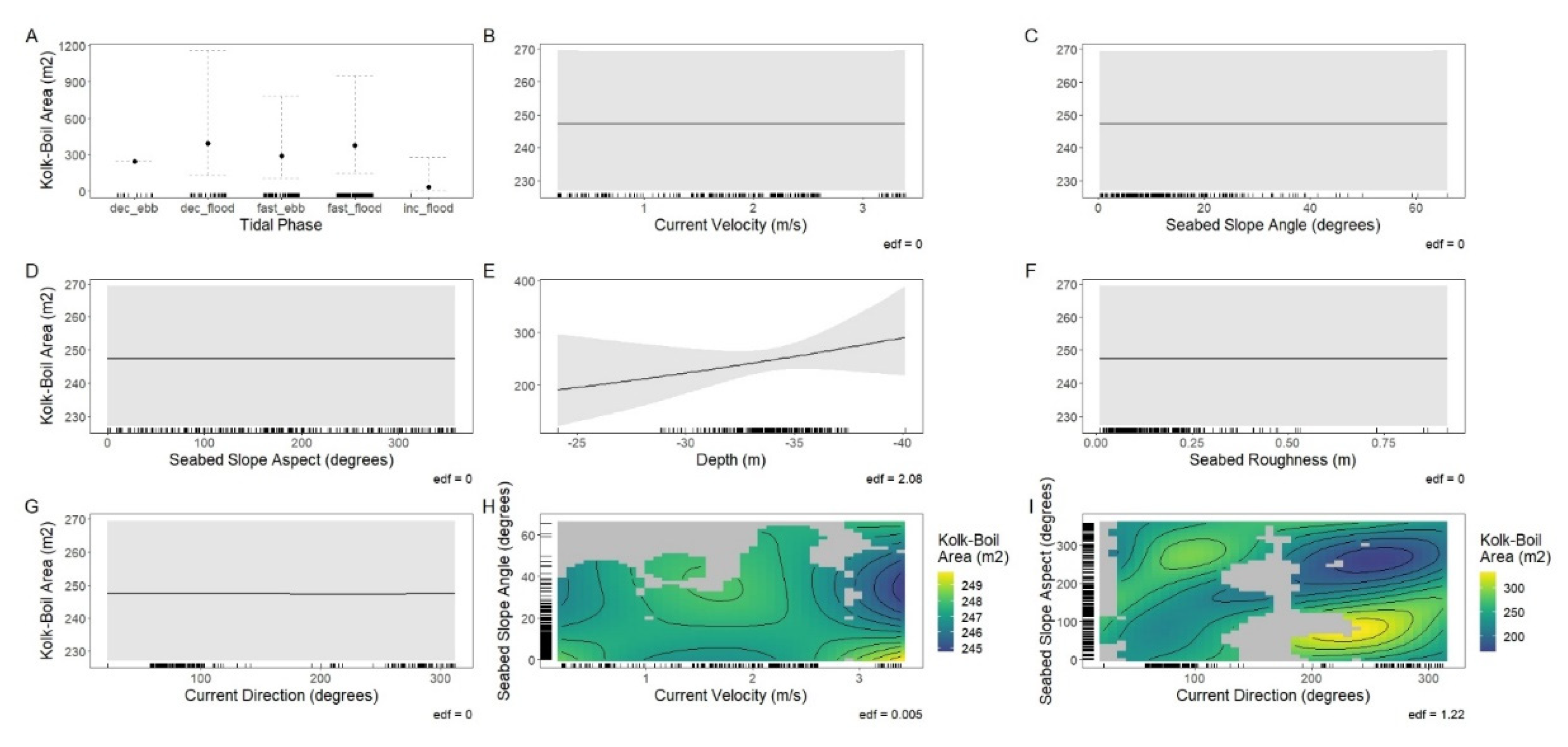
3.2. Kolk-Boil Presence

A total of 627 kolk-boil-present images (including formed and un-formed boils) were recorded. When split via tidal phase, the greatest counts were logged in fast-ebb (71) and fast-flood (176) periods (Figure 7A). While the mean absolute current speed across the data was 1.44 m/s, 44% of kolk-boils occurred at absolute current velocities exceeding, or equal to, 2.0 m/s (Figure 7B). Peaks in boil presence were also observed at current directions going towards approx. 260–310° (n = 169) and approx. 50–110° (n = 362) (Figure 7C).
When examining bathymetric covariates, kolk-boil presence predominantly occurred between depths of 32–36 m (n = 533) (Figure 7D). Seabed slope angle, at boil locations, ranged from 0.20 to 65.84°; however, 80% fell between 0 and 20° (Figure 7E). Kolk-boil presence was marginally higher at seabed slope aspects approx. 130–210° (n = 145) but was generally evenly distributed across all aspect angles (Figure 7F). Kolk-boils occurred at the surface across a range of seabed roughness values (0.01–0.91 m), with 90% falling within a range of 0–0.25 m (Figure 7G).
The final model for kolk-boil presence included current velocity, depth, seabed slope angle, current direction, tidal phase, and the two-way interactions of current velocity/seabed slope angle and current direction/seabed slope aspect as explanatory variables, with Flight ID as a random effect variable (Table 2). The model fit (30.2% deviance explained) highlighted that current velocity had a significant effect on kolk-boil presence (p ≤ 0.001) (Figure 8A). Probability slightly increased when moving from 0–2.0 m/s, whereupon a sharp rise was observed beyond this, with likelihood of presence reaching > 99% beyond 3.0 m/s (Figure 8A). Comparatively, a marginal effect was observed with depth (p = 0.003), with probability of presence increasing past 25 m, peaking at approx. 36–37 m, and then beginning to decline beyond this point (Figure 8B). Similarly, seabed slope angle was marginally influential in explaining boil presence (p = 0.04) showing a slight decrease in probability of presence as slope angle increased from 0–80° (Figure 8C). Current direction highlighted slight peaks at approx. 0° and 300°, where the probability of kolk-boil presence was slightly greater (Figure 8D), but this was not deemed significant (p = 0.22). Finally, limited variation was observed in the probability of boil presence between differing tidal phases (Figure 8E).
The two-way interaction of both current velocity and seabed slope angle was significant (p = 0.002). This interaction emphasised that at lower current velocities (<1 m/s) increased slope angle (60–80°) appeared to play an important role in predicting kolk-boil presence, while at faster velocities (> 3.0 m/s) probability of occurrence was dependent on slightly shallower gradients (40–60°) (Figure 8F). The final two-way interaction of seabed slope aspect and current direction (p = 0.04) highlighted approximate opposing combinations where the probability of boil presence would be higher. This included seabed slope aspects of approx. 200° with current direction towards approx. 80°, and seabed slope aspects approx. 60° with current direction towards approx. 330° (Figure 8G).

4. Discussion

4.1. Kolk-Boil Characterisation

To our knowledge, this study is the first of its kind to collect in situ detail of fine-scale characteristics of kolk-boils at the surface and relate them to physical properties, within a tidal stream environment, using UAV imagery. This study provides detailed information on formed kolk-boil surface distribution within the Inner Sound of the Pentland Firth and found visible spatial patterns emerging when analysed based on tidal phase (the combination of current velocity and direction) (Figure 6). Kolk-boil distribution was heavily influenced by tidal phase, with specific spatial clustering observed dependent on the prevailing ebb or flood periods. While several environmental covariates significantly impacted presence at the surface, current velocity appeared to be the most influential in allowing for the ability to reliably predict feature occurrence at the surface. This was consistently observable at velocities >3.0 m/s, where the probability of kolk-boil presence was >99%.

4.1.1. Distribution

While kolk-boil formation has been quantified in both theoretical, laboratory and field settings, empirical observations in the marine environment at the surface have remained mostly qualitative with only limited attempts to characterise distribution [18,19,22,25,46]. Nevertheless, there is consistency in highlighting that kolk-boil eruptions occur downstream from the area of formation [22,46,47,48]. Kolk-boils have been observed to travel at a slower rate than the surrounding water during advection, with the prevailing current speed and direction thought to influence kolk-boil eruption points at the surface [19]. More recent studies, using high-resolution particle image velocimetry (PIV) within a laboratory setting, also corroborate these previously described relationships of variation in the location of kolk-boil eruption in response to water depth, mean flow velocity and bathymetry [20,49]. However, kolk-boil movement is not just limited to within the water column. Within river environments, kolk-boils have also been observed to propagate downstream while at the surface, remaining both visible and maintaining their form over “tens of metres” [50].
The accelerated current velocities present in tidal stream environments, often more than 2 m/s, are thus theorised by this paper to be the main contributor to the distribution of formed kolk-boils at the surface. Our analysis corroborates these findings when examining the distribution of formed kolk-boils relative to tidal phase, with those detected in ebb and flood phases displaying clear spatial clustering (Figure 6). It is also likely that kolk-boils will travel a greater distance, either through the water column or while at the surface, dependent on current velocity and current direction. This indicates that, although turbulence is a stochastic phenomenon, the distribution of kolk-boils on the surface (within a tidal stream environment) is predictable in space and time.

4.1.2. Presence

Within this study the interaction of current velocity and seabed slope angle were found to significantly influence kolk-boil presence at the surface, with the combinations of slower speeds/greater slope angles and faster speeds/shallower slope angles creating the highest likelihood of kolk-boil presence (Figure 8F). It has been highlighted, within laboratory settings, that the presence of bed inclination downstream of the separation zone increases the occurrence of ejection events, compared to a flat surface, that are increasingly likely to rise further through the water column [51]. It is therefore reasonable to theorise that, within real conditions, the gradient of the reattachment zone, in conjunction with current velocity, plays a significant role in determining how likely a kolk-boil is to be present at the surface. At slower velocities (<0.5 m/s), high slope angle may compensate for the lack of momentum and ensure a kolk’s trajectory through the water column is steep enough to allow it to manifest at the surface as a boil. However, at faster current speeds (>3.0 m/s) it can be conceived that the increased energy lowers the requirement of a steep gradient (by approx. 20°), beyond the separation zone, enough to ensure kolk-boil presence at the surface. This may also provide sound reasoning for the relationship that was observed between kolk-boil presence and depth (Figure 8B). An increased depth may allow for the kolk to fully form within the water column, compared to more shallow water where it may not have the necessary vertical space required to gain momentum and breach the surface. However, further work would need to be carried out on the specifics of these complex relationships, as this paper only highlights the significance of these interactions regarding the probability of kolk-boil presence at the surface.
Current velocity was highly influential in determining kolk-boil presence at the surface, particularly at speeds >3.0 m/s, and in turn towards the overall characterisation of these features (Figure 8A). Within a tidal stream environment, turbulence is governed by the energy created from tidal flows, and therefore the larger the energy input (e.g., faster current velocities) the greater proportion available for the creation of turbulent structures [8]. Laboratory studies observing flow over materials with different surface roughness values also highlighted that an increase in current velocity caused a concurrent intensification in the occurrence of “multi-ejection” events into the water column, with the height and period of these ejections also becoming greater as flow speed increased [52]. It is therefore possible to assume that when current velocity increases, the probability of kolk-boil presence will also significantly rise as more turbulent kinetic energy is available within the system. With the probability of kolk-boil presence almost a certainty at the fastest current velocities recorded within this study (>3.0 m/s), it highlights the ability to characterise such features, at the surface, not just spatially but also temporally. In doing so, kolk-boil presence can move from being random turbulent events to a phenomenon that is now, with the aid of UAV imagery, increasingly likely to be predictable. Future work will investigate further sites to consider the transferability of these relationships and the influence of differences in bathymetry and flow regimes.

4.2. Implications for Tidal Energy Developments

To date, there are limited examples of empirical studies of fine-scale turbulence characterisation within tidal stream environments, with most approaches using model simulations [53]. However, increased turbulence will intensify device power fluctuations compared to laminar flow conditions [11]. This non-uniformity will have an impact on device reliability, increasing fatigue loading due to greater variation in flow, causing fluctuations to the amplitude of force applied to turbines [54]. It is therefore evident, and commercially important, that developers carry out representative assessments of the turbulent characteristics of a site to manage operation and to better inform device siting [55]. This information is also important in determining the correct materials and designs required for optimal turbine longevity and reliability within turbulent conditions [9].
While it is accepted that kolk-boils are complex, three dimensional, phenomena that occur throughout the water column, the findings of this study provide the basis for accurate characterisation of the feature at the surface. These results can allow tidal energy developers a simple method in which to predict where, and when, kolk-boils are likely to be present and to visually map distribution across a site. This approach is highly novel in terms of the fine-scale resolution at which turbulent feature characterisation can occur, which has not been seen in existing methods. UAV imagery, to characterise kolk-boils, provides an alternative, and complementary, perspective from which relevant information can be gained. Consequently, the findings of this paper can be used to support present and future tidal energy developments, worldwide, in being cost effective, efficient, and remaining a relevant part of the overall MRE sector. The methodology demonstrated also highlights the suitability of UAVs as a survey platform for fine-scale hydrodynamic surveys within tidal stream environments. This is due to the ability to carry out lower-cost, replicable and standardised surveys with simpler logistics, the ability to be used across multiple tidal stream sites and reduced risk to personnel compared to other in situ data collection methods [13]. The scale of monitoring (metres and seconds) and coverage per image is deemed appropriate, as all kolk-boils were accurately characterised within a single image, including boils with areas >1000 m2 (Figure A1).
It is also important to note the ecological implications. Tidal stream environments are foraging hotspots for top predator species (seabirds and marine mammals), with turbulent features such as kolk-boils, heavily influencing their usage patterns due to effects on availability of prey [8,12,13]. The potential ecological impacts of tidal stream energy technologies can be significant constraints on the licensing of developments. Therefore, improved understanding of how animals interact with these environments is key to better quantifying potential effects. Within the MRE sector, ecological impact assessment protocols and post-deployment monitoring are still being refined compared to other established industries, with the need for cumulative approaches that take into account hydrodynamic, prey and predator interactions becoming increasingly evident [56,57,58,59]. Empirical data collection of kolk-boil characteristics, and other turbulent features within tidal stream environments, are the basis of habitat characterisation that is needed to begin furthering these cumulative approaches and understanding regarding the bio-physical interactions occurring within the habitats [60]. UAVs offer an inexpensive method to achieve this by being able to simultaneously collect relevant fine-scale surface hydrodynamic and fauna data reliably across multiple sites. This is needed to understand the potential environmental effects of tidal energy devices for both regulators and developers regarding the development, siting and operation of future and current tidal energy devices [57].

4.3. Future Work

While it was beyond the scope of this paper to incorporate the type of data and analysis needed to identify correlations between boil presence and lagged upstream seabed slope angle and aspect values, it is believed to be a necessary next step. The use of active acoustic devices has already seen success in the detailing of turbulence within the water column and would help to provide the required data [18,21,22,61]. Concurrent fine-scale measurements of kolk-boils at the surface and turbulence within the water column would facilitate analysis of the complete lifespan of the hydrodynamic feature from formation at the seabed to persistence at the surface. In turn, this would permit calculation of where a kolk-boil is likely to erupt, at the surface, based on its point of formation, seabed slope angle and current velocity.
The findings of this study indicate that future measurements should also focus on the potential influence that tidal turbines might have upon the creation, and characteristics, of kolk-boils as well as the exact implications of the feature on device power fluctuation. Increased characterisation, including other parameters such as area, would aid in this effort by allowing for a more complete comparison to be made between turbulence in the water column and the resultant output at the surface.

5. Conclusions

UAV imagery allowed for the characterisation of kolk-boils at the surface within a tidal stream environment. This study highlighted the feasibility of UAVs as a platform for cost-effective fine-scale hydrodynamic surveys and the ability to facilitate the prediction, both spatially and temporally, of “ephemeral” turbulent features at the surface. The methodology can provide standardised data across multiple sites, with relative logistic ease, and can be used individually or in conjunction with existing marine survey methods.
These findings have important implications for tidal turbine developers, and regulators, as they provide the ability to predict kolk-boil occurrence in space and time. This is important not just for design, development, and optimisation of tidal turbines, but also for the environmental consenting processes that are intrinsically linked due to animal use of hydrodynamic features for foraging opportunities.
Moving forward, the inclusion of further hydrodynamic feature characteristics at the surface, such as boil area and concurrent information from within the water column, would allow for the ability to better predict occurrence, distribution, and characterisation throughout an entire feature lifecycle. This would enable the effects of tidal turbines on fine-scale hydrodynamic processes within a site, and vice versa, to be increasingly understood and more accurately quantified.

Author Contributions

J.S.: Conceptualization, Methodology, Software, Formal analysis, Data Curation, Writing—Original Draft, Writing—Review and Editing, Visualization. B.E.S.: Conceptualization, Investigation, Writing—Review and Editing, Supervision, Project administration, Funding acquisition. L.K.: Conceptualization, Writing—Original Draft, Writing—Review and Editing, Supervision. J.M.: Methodology, Software, Investigation, Resources, Data Curation, Writing—Review and Editing, Supervision. J.W.: Conceptualization, Writing—Review and Editing, Supervision, Funding acquisition. A.C.: Investigation, Writing—Review and Editing, Software, Formal analysis. D.R.: Writing—Review and Editing, Software, Formal analysis. M.Y.: Methodology, Software, Writing—Review and Editing. B.J.W.: Conceptualization, Methodology, Software, Investigation, Resources, Data Curation, Writing—Review and Editing, Supervision, Project administration, Funding acquisition. All authors have read and agreed to the published version of the manuscript.

Funding

This work was funded by the Bryden Centre project, supported by the European Union’s INTERREG VA Programme, and managed by the Special EU Programmes Body (SEUPB). The views and opinions expressed in this paper do not necessarily reflect those of the European Commission or SEUPB. Aspects of this research were also funded by a Royal Society Research Grant [RSG\R1\180430], the NERC VertIBase project [NE/N01765X/1] and the UK Department for Business, Energy and Industrial Strategy’s offshore energy Strategic Environmental Assessment programme.

Institutional Review Board Statement

Not applicable.

Informed Consent Statement

Not applicable.

Data Availability Statement

The data underlying this article will be shared on reasonable request to the corresponding author.

Acknowledgments

We gratefully acknowledge the support of Julien Martin, colleagues at Marine Scotland Science and the crew and scientists of the MRV Scotia 2016 and 2018 cruises (particularly Chief Scientists Eric Armstrong and Adrian Tait). We also acknowledge the work contributed by ERI interns: Gael Gelis and Martin Forestier.

Conflicts of Interest

The authors declare no conflict of interest. The funders had no role in the design of the study; in the collection, analyses, or interpretation of data; in the writing of the manuscript, or in the decision to publish the results.

Appendix A

tan(VFOV/2) = Width[m]/2 × Altitude[m]
Width[m] = 2 × Altitude[m] × tan(VFOV/2
Calibration factor = Width[m]/Width[px] = 2 × Altitude[m] × tan(VFOV/2)/Width[px]
Equation (A3) Calibration factor equation used to convert an area covered by a pixel, within an image, into metres. This is based on the vertical field of view (VFOV), the width of the image in pixels, and the altitude of the UAV when the image was taken after relative (take off) altitude has been accounted for.
Figure A1. (A) The effect of current speed on formed boil area; (B) The effect of depth on formed boil area; (C) The effect of current direction on formed boil area; (D) The effect of tidal phase on formed boil area; (E) The effect of seabed slope angle on formed boil area; (F) The effect of seabed roughness on formed boil area; (G) The effect of seabed slope aspect on formed boil area.
Jmse 09 00484 g0a1
Figure A2. (AC) The effect of tidal phase, current velocity and seabed slope angle on kolk-boils area respec-tively; (DF) The effect of seabed slope aspect, depth and seabed roughness on kolk-boils area re-spectively; (G) The effect of current direction on kolk-boils area; (H) The effect current velocity on seabed slope angle; (I) The effect of current direction on seabed slope aspect.
Jmse 09 00484 g0a2
Figure A3. QQ and residual vs. fitted plots for kolk-boil presence model detailing a binomial distribution fits well and that there is no clear pattern in residuals.
Jmse 09 00484 g0a3
Figure A4. Over-dispersion plot for kolk-boil presence model. Given the fitted model (red line) is within the simulated values there was no dispersion.
Jmse 09 00484 g0a4
Figure A5. Residual vs. time and autocorrelation function (ACF) plots for kolk-boil presence. No temporal correlation is observed.
Jmse 09 00484 g0a5
Figure A6. QQ and residual vs. fitted plots for kolk-boil area model detailing a gaussian distribution fits well and that there is no clear pattern in residuals.
Jmse 09 00484 g0a6
Figure A7. Over-dispersion plot for kolk-boil area model. Given the fitted model (red line) is within the simulated values there was no dispersion.
Jmse 09 00484 g0a7
Figure A8. Residual vs. time and autocorrelation function (ACF) plots for kolk-boil area. No temporal correlation is observed.
Jmse 09 00484 g0a8

References

  1. Committee on Climate Change Net Zero: The UK’s Contribution to Stopping Global Warming. Available online: https://www.theccc.org.uk/publication/net-zero-the-uks-contribution-to-stopping-global-warming/ (accessed on 18 August 2020).
  2. Roche, R.C.; Walker-Springett, K.; Robins, P.E.; Jones, J.; Veneruso, G.; Whitton, T.A.; Piano, M.; Ward, S.L.; Duce, C.E.; Waggitt, J.J.; et al. Research priorities for assessing potential impacts of emerging marine renewable energy technologies: Insights from developments in Wales (UK). Renew. Energy 2016, 99, 1327–1341. [Google Scholar] [CrossRef] [Green Version]
  3. Pye, S.; Li, F.G.N.; Price, J.; Fais, B. Achieving net-zero emissions through the reframing of UK national targets in the post-Paris Agreement era. Nat. Energy 2017, 2, 1–7. [Google Scholar] [CrossRef]
  4. Wang, Z.; Carriveau, R.; Ting, D.S.K.; Xiong, W.; Wang, Z. A review of marine renewable energy storage. Int. J. Energy Res. 2019, 43, 6108–6150. [Google Scholar] [CrossRef]
  5. González-Gorbeña, E.; Rosman, P.C.C.; Qassim, R.Y. Assessment of the tidal current energy resource in São Marcos Bay, Brazil. J. Ocean Eng. Mar. Energy 2015, 1, 421–433. [Google Scholar] [CrossRef]
  6. Nachtane, M.; Tarfaoui, M.; Goda, I.; Rouway, M. A review on the technologies, design considerations and numerical models of tidal current turbines. Renew. Energy 2020, 157, 1274–1288. [Google Scholar] [CrossRef]
  7. Benjamins, S.; Van Geel, N.; Hastie, G.; Elliott, J.; Wilson, B. Harbour porpoise distribution can vary at small spatiotemporal scales in energetic habitats. Deep. Sea Res. Part II Top. Stud. Oceanogr. 2017, 141, 191–202. [Google Scholar] [CrossRef] [Green Version]
  8. Benjamins, S.; Dale, A.; Hastie, G.; Waggitt, J.J.; Lea, M.-A.; Scott, B.; Wilson, B. Confusion Reigns? A Review of Marine Megafauna Interactions with Tidal-Stream Environments. Oceanogr. Mar. Biol. Annu. Rev. 2015, 53, 1–54. [Google Scholar] [CrossRef]
  9. Thiébaut, M.; Filipot, J.-F.; Maisondieu, C.; Damblans, G.; Duarte, R.; Droniou, E.; Chaplain, N.; Guillou, S. A comprehensive assessment of turbulence at a tidal-stream energy site influenced by wind-generated ocean waves. Energy 2020, 191, 116550. [Google Scholar] [CrossRef]
  10. Ikhennicheu, M.; Germain, G.; Druault, P.; Gaurier, B. Experimental study of coherent flow structures past a wall-mounted square cylinder. Ocean Eng. 2019, 182, 137–146. [Google Scholar] [CrossRef]
  11. Sentchev, A.; Thiébaut, M.; Schmitt, F.G. Impact of turbulence on power production by a free-stream tidal turbine in real sea conditions. Renew. Energy 2020, 147, 1932–1940. [Google Scholar] [CrossRef]
  12. Whitton, T.A.; Jackson, S.E.; Hiddink, J.G.; Scoulding, B.; Bowers, D.; Powell, B.; D’Urban Jackson, T.; Gimenez, L.; Davies, A.G. Vertical migrations of fish schools determine overlap with a mobile tidal stream marine renewable energy device. J. Appl. Ecol. 2020, 57, 729–741. [Google Scholar] [CrossRef]
  13. Williamson, B.; Fraser, S.; Williamson, L.; Nikora, V.; Scott, B. Predictable changes in fish school characteristics due to a tidal turbine support structure. Renew. Energy 2019, 141, 1092–1102. [Google Scholar] [CrossRef]
  14. Dufaur, J. Characteristics of the turbulent flow in the Inner Sound, tidal development site in the Pentland Firth, Scotland. Master’s Thesis, University of Aberdeen, Aberdeen, Scotland, 2016. [Google Scholar]
  15. Matthes, G.H. Macroturbulence in natural stream flow. Trans. Am. Geophys. Union 1947, 28, 255–265. [Google Scholar] [CrossRef]
  16. Ikhennicheu, M.; Druault, P.; Gaurier, B.; Germain, G. An experimental study of bathymetry influence on turbulence at a tidal stream site. In Proceedings of the 12th European Wave and Tidal Energy Conference, Cork, Ireland, 27 August–1 September 2017. [Google Scholar]
  17. Müller, A.; Gyr, A. On the vortex formation in the mixing layer behind dunes. J. Hydraul. Res. 1986, 24, 359–375. [Google Scholar] [CrossRef]
  18. Thorpe, S.A.; Green, J.A.M.; Simpson, J.H.; Osborn, T.R.; Nimmo Smith, W.A.M. Boils and Turbulence in a Weakly Stratified Shallow Tidal Sea. J. Phys. Oceanogr. 2008, 38, 1711–1730. [Google Scholar] [CrossRef]
  19. Best, J.L. Kinematics, Topology and Significance of Dune-Related Macroturbulence: Some Observations from the Laboratory and Field. Fluv. Sedimentol. VII 2009, 35, 41–60. [Google Scholar] [CrossRef]
  20. Best, J. The fluid dynamics of river dunes: A review and some future research directions. J. Geophys. Res. Earth Surf. 2005, 110, 1–21. [Google Scholar] [CrossRef]
  21. Sellar, B.; Harding, S.; Richmond, M. High-resolution velocimetry in energetic tidal currents using a convergent-beam acoustic Doppler profiler. Meas. Sci. Technol. 2015, 26, 085801. [Google Scholar] [CrossRef]
  22. Nimmo Smith, W.A.M.; Thorpe, S.A.; Graham, A. Surface effects of bottom-generated turbulence in a shallow tidal sea. Nature 1999, 400, 251–254. [Google Scholar] [CrossRef]
  23. Kregting, L.; Elsaesser, B.; Kennedy, R.; Smyth, D.; O’Carroll, J.; Savidge, G. Do Changes in Current Flow as a Result of Arrays of Tidal Turbines Have an Effect on Benthic Communities? PLoS ONE 2016, 11, e0161279. [Google Scholar] [CrossRef] [Green Version]
  24. Marmorino, G.O.; Smith, G.B.; Miller, W.D. Turbulence characteristics inferred from time-lagged satellite imagery of surface algae in a shallow tidal sea. Cont. Shelf Res. 2017, 148, 178–184. [Google Scholar] [CrossRef]
  25. Chickadel, C.C.; Horner-Devine, A.R.; Talke, S.A.; Jessup, A.T. Vertical boil propagation from a submerged estuarine sill. Geophys. Res. Lett. 2009, 36, 1–6. [Google Scholar] [CrossRef] [Green Version]
  26. Easton, M.C.; Woolf, D.K.; Bowyer, P.A. The dynamics of an energetic tidal channel, the Pentland Firth, Scotland. Cont. Shelf Res. 2012, 48, 50–60. [Google Scholar] [CrossRef]
  27. Waldman, S.; Bastón, S.; Nemalidinne, R.; Chatzirodou, A.; Venugopal, V.; Side, J. Implementation of tidal turbines in MIKE 3 and Delft3D models of Pentland Firth & Orkney Waters. Ocean Coast. Manag. 2017, 147, 21–36. [Google Scholar] [CrossRef] [Green Version]
  28. Neill, S.P.; Vögler, A.; Goward-Brown, A.J.; Baston, S.; Lewis, M.J.; Gillibrand, P.A.; Waldman, S.; Woolf, D.K. The wave and tidal resource of Scotland. Renew. Energy 2017, 114, 3–17. [Google Scholar] [CrossRef]
  29. Wang, T.; Adcock, T.A. Power and thrust capping of tidal stream turbines—A case study of the pentland firth. In Proceedings of the International Conference on Offshore Mechanics and Arctic Engineering—OMAE; American Society of Mechanical Engineers: New York, NY, USA, 2018; Volume 10. [Google Scholar]
  30. Goddijn-Murphy, L.; Woolf, D.K.; Easton, M.C. Current Patterns in the Inner Sound (Pentland Firth) from Underway ADCP Data. J. Atmos. Ocean. Technol. 2013, 30, 96–111. [Google Scholar] [CrossRef]
  31. Rajgor, G. Tidal developments power forward. Renew. Energy Focus 2016, 17, 147–149. [Google Scholar] [CrossRef]
  32. Policy and Innovation Group UK Ocean Energy Review 2019. Available online: http://www.policyandinnovationedinburgh.org/uploads/3/1/4/1/31417803/policy_and_innovation_group_uk_oceanenergy_review_2019._final.pdf (accessed on 18 August 2020).
  33. SIMEC MeyGen|Tidal Projects|SIMEC Atlantis Energy. Available online: https://simecatlantis.com/projects/meygen/ (accessed on 17 July 2020).
  34. Griffiths, T.; Draper, S.; Cheng, L.; Tong, F.; Fogliani, A.; White, D.; Johnson, F.; Coles, D.; Ingham, S.; Lourie, C. Subsea Cable Stability on Rocky Seabeds: Comparison of Field Observations Against Conventional and Novel Design Methods. In Proceedings of the International Conference on Offshore Mechanics and Arctic Engineering—OMAE, New York, NY, USA, 30 December 2018; American Society of Mechanical Engineers: New York, NY, USA, 2018; Volume 5. [Google Scholar]
  35. Colefax, A.P.; Butcher, P.A.; Kelaher, B.P. The potential for unmanned aerial vehicles (UAVs) to conduct marine fauna surveys in place of manned aircraft. ICES J. Mar. Sci. 2018, 75, 1–8. [Google Scholar] [CrossRef]
  36. Hodgson, J.C.; Koh, L.P. Best practice for minimising unmanned aerial vehicle disturbance to wildlife in biological field research. Curr. Biol. 2016, 26, R404–R405. [Google Scholar] [CrossRef] [PubMed] [Green Version]
  37. Civil Aviation Authority UK CAA Drone Code. Available online: https://dronesafe.uk/wp-content/uploads/2019/11/Drone-Code_October2019.pdf (accessed on 18 August 2020).
  38. DJI. DJI Phantom 4 Pro—Specs, Tutorials & Guides—DJI. Available online: https://www.dji.com/uk/phantom-4-pro/info#specs (accessed on 17 July 2020).
  39. Longuet-Higgins, M.S. Surface manifestations of turbulent flow. J. Fluid Mech. 1996, 308, 15–29. [Google Scholar] [CrossRef]
  40. McIlvenny, J.; Williamson, B.J.; MacDowall, C.; Gleizon, P.; O’Hara Murray, R. Modelling hydrodynamics of fast tidal stream around a promontory headland. 2021; in review. [Google Scholar]
  41. Zamon, J.E. Mixed species aggregations feeding upon herring and sandlance schools in a nearshore archipelago depend on flooding tidal currents. Mar. Ecol. Prog. Ser. 2003, 261, 243–255. [Google Scholar] [CrossRef]
  42. QGIS 23.2.1. Raster Analysis—QGIS Documentation. Available online: https://docs.qgis.org/3.10/en/docs/user_manual/processing_algs/gdal/rasteranalysis.html?highlight=roughness#roughness (accessed on 18 August 2020).
  43. Wood, S.N. Fast stable restricted maximum likelihood and marginal likelihood estimation of semiparametric generalized linear models. J. R. Stat. Soc. Ser. B Stat. Methodol. 2010, 73, 3–36. [Google Scholar] [CrossRef] [Green Version]
  44. Pedersen, E.J.; Miller, D.L.; Simpson, G.L.; Ross, N. Hierarchical generalized additive models in ecology: An introduction with mgcv. PeerJ 2019, 7, e6876. [Google Scholar] [CrossRef] [PubMed] [Green Version]
  45. Marra, G.; Wood, S.N. Practical variable selection for generalized additive models. Comput. Stat. Data Anal. 2011, 55, 2372–2387. [Google Scholar] [CrossRef]
  46. Kadota, A.; Nezu, I. Three-dimensional structure of space-time correlation on coherent vortices generated behind dune crest. J. Hydraul. Res. 1999, 37, 59–80. [Google Scholar] [CrossRef]
  47. Stoesser, T.; Braun, C.; García-Villalba, M.; Rodi, W. Turbulence Structures in Flow over Two-Dimensional Dunes. J. Hydraul. Eng. 2008, 134, 42–55. [Google Scholar] [CrossRef]
  48. Nezu, I.; Tominaga, A.; Nakagawa, H. Field Measurements of Secondary Currents in Straight Rivers. J. Hydraul. Eng. 1993, 119, 598–614. [Google Scholar] [CrossRef]
  49. Kwoll, E.; Venditti, J.G.; Bradley, R.W.; Winter, C. Observations of Coherent Flow Structures Over Subaqueous High- and Low- Angle Dunes. J. Geophys. Res. Earth Surf. 2017, 122, 2244–2268. [Google Scholar] [CrossRef]
  50. Kostaschuk, R.A.; Church, M.A. Macroturbulence generated by dunes: Fraser River, Canada. Sediment. Geol. 1993, 85, 25–37. [Google Scholar] [CrossRef]
  51. Ikhennicheu, M.; Gaurier, B.; Druault, P.; Germain, G. Experimental analysis of the floor inclination effect on the turbulent wake developing behind a wall mounted cube. Eur. J. Mech. B/Fluids 2018, 72, 340–352. [Google Scholar] [CrossRef] [Green Version]
  52. Mao, Y. The effects of turbulent bursting on the sediment movement in suspension. Int. J. Sediment Res. 2003, 18, 148–157. [Google Scholar]
  53. Mercier, P.; Grondeau, M.; Guillou, S.; Thiébot, J.; Poizot, E. Numerical study of the turbulent eddies generated by the seabed roughness. Case study at a tidal power site. Appl. Ocean Res. 2020, 97, 102082. [Google Scholar] [CrossRef]
  54. Blackmore, T.; Myers, L.E.; Bahaj, A.S. Effects of turbulence on tidal turbines: Implications to performance, blade loads, and condition monitoring. Int. J. Mar. Energy 2016, 14, 1–26. [Google Scholar] [CrossRef] [Green Version]
  55. Osalusi, E.; Side, J.; Harris, R. Structure of turbulent flow in EMEC’s tidal energy test site. Int. Commun. Heat Mass Transf. 2009, 36, 422–431. [Google Scholar] [CrossRef]
  56. Scherelis, C.; Penesis, I.; Hemer, M.A.; Cossu, R.; Wright, J.T.; Guihen, D. Investigating biophysical linkages at tidal energy candidate sites: A case study for combining environmental assessment and resource characterisation. Renew. Energy 2020, 159, 399–413. [Google Scholar] [CrossRef]
  57. Shields, M.A.; Woolf, D.K.; Grist, E.P.; Kerr, S.A.; Jackson, A.C.; Harris, R.E.; Bell, M.C.; Beharie, R.; Want, A.; Osalusi, E.; et al. Marine renewable energy: The ecological implications of altering the hydrodynamics of the marine environment. Ocean Coast. Manag. 2011, 54, 2–9. [Google Scholar] [CrossRef]
  58. Waggitt, J.J.; Scott, B.E. Using a spatial overlap approach to estimate the risk of collisions between deep diving seabirds and tidal stream turbines: A review of potential methods and approaches. Mar. Policy 2014, 44, 90–97. [Google Scholar] [CrossRef] [Green Version]
  59. Isaksson, N.; Masden, E.A.; Williamson, B.J.; Costagliola-Ray, M.M.; Slingsby, J.; Houghton, J.D.R.; Wilson, J. Assessing the effects of tidal stream marine renewable energy on seabirds: A conceptual framework. Mar. Pollut. Bull. 2020, 157, 111314. [Google Scholar] [CrossRef]
  60. Johnston, D.T.; Furness, R.W.; Robbins, A.M.C.; Tyler, G.; Taggart, M.A.; Masden, E.A. Black guillemot ecology in relation to tidal stream energy generation: An evaluation of current knowledge and information gaps. Mar. Environ. Res. 2018, 134, 121–129. [Google Scholar] [CrossRef]
  61. Williamson, B.J.; Fraser, S.; Blondel, P.; Bell, P.S.; Waggitt, J.J.; Scott, B.E. Multisensor Acoustic Tracking of Fish and Seabird Behavior around Tidal Turbine Structures in Scotland. IEEE J. Ocean. Eng. 2017, 42, 948–965. [Google Scholar] [CrossRef] [Green Version]
Figure 1. A schematic detailing kolk formation on the seabed.
Jmse 09 00484 g001
Figure 3. The United Kingdom and the Inner Sound of the Pentland Firth.
Jmse 09 00484 g003
Figure 4. UAV coverage, over ground, of surveys split across (a) ebb and (b) flood tidal phases for 2016 and 2018 combined.
Jmse 09 00484 g004
Figure 5. Example kolk-boils from UAV imagery and the difference between “formed” and un-formed” categorisations, with the red line indicating the visible part of the boil perimeter.
Jmse 09 00484 g005
Figure 6. The distribution of formed kolk-boils, based on tidal phase, within the Inner Sound from 2016 and 2018 combined. Flood tidal flow is in an easterly direction, ebb flow in a westerly direction. Grey shaded area represents UAV coverage over ground, with black dots highlighting tidal turbine positions.
Jmse 09 00484 g006
Figure 7. Cumulative counts of kolk-boil presence (an image with a kolk-boil in it) and absence (an image without a kolk-boil in it) in relation to tidal phase (A), current velocity (B), current direction (C), depth (D), seabed slope angle (E), seabed slope aspect (F) and seabed roughness (G). Bars for kolk-boil presence (green) and absence (grey) are stacked.
Jmse 09 00484 g007
Figure 8. GAM relationships for kolk-boil presence are shown. (AE) show the effect of current velocity, depth, seabed slope angle, current direction and tidal phase on the predicted probability of kolk-boil presence, whereas this is coloured in (F,G) highlighting the two-way interaction effect of current velocity with seabed slope angle, and current direction with seabed slope aspect. The dashed lines in (E) and shaded areas of (AD) represent the 95% confidence intervals. In all plots data are represented by the rug tick marks.
Jmse 09 00484 g008
Table 1. Comparison of UAV and camera specifications between 2016 and 2018 surveys.
UAV and Camera Specifications20162018
UAV SwellPro SplashDrone 3+DJI Phantom 4 Advanced V2.0
CameraGoPro HERO4 Black (12 MP)1-inch CMOS Sensor (20 MP)
Aspect Ratio4:3 (4000 × 3000 pixels)3:2 (5472 × 3648 pixels)
Average Relative Altitude Flown (m)46 70
Image Type TakenJPEGSimultaneous pairs of RAW and JPEG
Sampling Interval between Images/Image Pairs (Seconds)1 (subsampled to match 2018 data)5
Average Image Area (m2)5119.5611,577.52
Table 2. Variables included in the final kolk-boil presence model (excluding those penalised) identified using GAMs with a significance level of p < 0.05. For parametric coefficients, which are presented on the logit scale, estimate, standard error (Std. error), z-values (z), and p-values (p) are shown. For smooth terms, the estimated degrees of freedom (EDF), chi-squared (Chi.sq) and p-values (p) are shown.
Parametric Coefficients:Model Summary:
Tidal Phase: Decreasing Ebb (Intercept, α0) Estimate = −1.627
Std. Error = 1.425
z = −1.141
p = 0.254
Tidal Phase: Decreasing Flood (α1)Estimate = −0.747
Std. Error = 1.715
z = −0.435
p = 0.663
Tidal Phase: Fast Ebb (α2)Estimate = −2.410
Std. Error = 1.586
z = −1.519
p = 0.129
Tidal Phase: Fast Flood (α3)
Tidal Phase: Increasing Flood (α4)
Estimate = −3.113
Std. Error = 1.560
z = −1.996
p = 0.046
Estimate = −3.808
Std. Error = 2.529
z = −1.506
p = 0.132
Smooth Terms:
Current Velocity ( f 1 )EDF = 6.093
Chi.sq = 24,747.999
p ≤ 0.001
Seabed Slope Angle ( f 2 )EDF = 7.567 × 10⁻¹
Chi.sq = 3.903
p = 0.039
Depth ( f 3 )EDF = 1.878
Chi.sq = 142.214
p = 0.003
Current Direction ( f 5 )EDF = 5.887 × 10⁻¹
Chi.sq = 5.611
p = 0.221
Current Velocity/ Seabed Slope Angle ( f 7 )EDF = 1.633
Chi.sq = 13.378
p = 0.002
Current Direction/ Seabed Slope Aspect ( f 8 )EDF = 2.119
Chi.sq = 5.878
p = 0.042
R2 (adj.) = 0.203 Deviance explained = 30.2%
n = 7236
Publisher’s Note: MDPI stays neutral with regard to jurisdictional claims in published maps and institutional affiliations.

