Astronomical Tide and Storm Surge Signals Observed in an Isolated Inland Maar Lake Near the Coast

Abstract

Aimed at the explanation of clear tidal signal and storm surge signals in a closed inland lake near the coast (the Huguangyan Lake), this work uses a combined approach with observations and model experiments. Huguangyan Lake is a closed inland freshwater coneless volcanic crater lake near the coast in tropical southern China, less than 5 km from an estuary. It has a diameter of about 1.5 km and relatively deep water of up to 20 m. Bottom pressure was measured from an acoustic Doppler current profiler (ADCP) for 10 days in September 2018 and 10 days in January 2019. The observations encompass the period of Typhoon Mangkhut, which passed the region when it made its landfall. The time series demonstrate clear tidal and subtidal signals. The tidal signal remains even if we exclude the barometric pressure effect. Interestingly, the lake has no surface connection with the ocean. The astronomical tide has an amplitude of about 2 cm. The major tidal signals include the principal solar semidiurnal (S2) and lunisolar (K1) constituents. During the passage of Typhoon Mangkhut, the water level variability inside the lake increased by an order of magnitude (>0.3 m). To examine whether the lake water level change was due to the natural oscillations inside the lake (or seiche), a numerical wind-driven hydrodynamics model was designed using the 3-D Finite Volume Community Ocean Model (FVCOM). The results show that a small first-order seiche can be generated, but only with a time scale of minutes and with a magnitude much smaller than the observed surface elevation changes. This excludes any measurable seiche and the observed surface elevation change inside the lake cannot be wind-driven. Moreover, tides inside the lake are not generated by tidal potential, as the lake is too small for having a locally generated tide. The main result of our study has therefore excluded the local tidal-generating force, wind-driven seiche, and barometric effect, as possible causes of the lake oscillation which has tidal and subtidal signals. The subtidal variation is at least one order of magnitude greater than tides inside the lake and is caused by weather-induced overall coastal ocean water level oscillations transmitted into the lake through groundwater connection. All these lead to the major conclusion that the lake is connected to the coastal ocean through groundwater.

1. Introduction

A maar lake is a freshwater lake formed by groundwater and/or precipitation filling an ancient volcanic depression. The distinction of maar lakes from other crater lakes are their low-relief terrain, because the corresponding volcanic explosion occurred in plains and the eruption led to a direct contact of groundwater with hot lava or magma. Typical maar lakes have horizontal scales between 60 and 8000 m with a water depth of 10 to 200 m. If a maar lake is not connected with the coastal ocean, it should not have any tidal signal, as tidal potential in such a small system is negligible.

The Huguangyan Lake is a maar lake (21°9′ N, 110°17′ E) near the coastline of tropical Southern China at the Leizhou Peninsula (Figure 1). It is a closed system with a shape of a heart (Figure 1). The east-west extent is about 1.8 km and the north-south extent is about 1.3 km. The average diameter is about 1.5 km. It has relatively deep water of up to 22 m with a mean depth of about 12 m [1]. It has no surface connection with the ocean and is located less than 5 km from the brackish estuarine water (an open channel in Guangzhou Bay), and it is completely fresh. It was formed by volcanic explosions about 140,000–160,000 years ago [2]. The isolated environment of Huguangyan Lake makes it an excellent sedimentation archive to study palaeoclimatology and environmental variations [3].

The region is dominated by East Asian monsoon and is also frequently affected by extreme weather events such as tropical cyclones. Studies on the Huguangyan Maar Lake in the past mainly focused on the impact of climate change, environmental change, and monsoon variations in Holocene and geologic ages, using lacustrine sediment core analysis [3,4,5,6,7]. However, there has been a lack of study on the physical properties, especially the hydrodynamics and circulations in this small system. The hydrodynamic processes, however, play a key role in the sedimentation and ecological processes in the system. Recent observations [8] show that the lake is filled with freshwater, and the temperature in winter and spring varies from 19 to 26 °C.

The study of astronomical tides in freshwater lakes without a surface connection with the ocean has only been reported in a limited number of publications. In [9], small tidal variations were shown in Lake Constance, located at the border of Germany, Switzerland and Austria, as a result of tide-generating force. Lake Constance is an elongated rectangular basin of freshwater with a surface area of 536 km², a dimension of 60 km × 11 km, and a maximum depth of more than 250 m, which is a much larger system with 5000 times greater volume and an order of magnitude deeper water compared to Huguangyan Lake. Their study applied an approximation based on the Laplace tidal equations (linear shallow water equation with Coriolis force) to the system and derived a prediction of astronomical tides with overestimated magnitude but good agreement of phase with observations. Astronomical tides in this deep lake are only on the order of a millimeter. In a more recent study [10], it also reported lunar tides in another elongated lake (37 km × 1.6 km, with a maximum depth of 227 m) in Loch Ness, Scotland, and the principal tidal constituent observed has an amplitude of 1.5 mm. The lake is not directly connected to the open ocean. Its M2 tidal signal is suggested to be from tidal loading related to the elastic change of the solid Earth under tidal forcing. The tide-potential effect in that lake is negligible. In contrast, astronomical tides in large freshwater lakes can be much more substantial and have been studied extensively. For example, the diurnal and semi-diurnal tides in the Great Lakes of North America, i.e., Lake Michigan, Lake Superior [11,12], Lake Ontario [13,14], and Lake Erie [15], have been subjects of many studies [16]. However, there has been essentially no report on tides in a freshwater lake of a much smaller size such as Huguangyan Lake, which has an order of magnitude shallower water but with a tidal signal an order of magnitude greater than those lakes with 5000 times greater volume (e.g., Lake Constance). Apparently, it is impossible for a much smaller and shallower freshwater lake to have a much larger tidal signal originating purely from tidal potential of the Moon and Sun or from the solid Earth’s elastic tidal deformation.

The objective of this study is to analyze water level data measured in the Huguangyan Lake and determine if tidal signals exist in the lake. We also investigate the mechanisms of tidal and subtidal signals of surface water level variations. In the following section, we discuss the study site and observations, followed by a discussion of results of the data analysis and a numerical model experiment using the Finite Volume Community Ocean Model (FVCOM) for an examination of seiche driven by wind before we present the conclusions.

2. Materials and Methods

The freshwater tropical Huguangyan Lake (Figure 1) is nearly circular with the shape of a heart when we look at its outline as well as its bathymetric contours: it is composed of two parts with an extremely shallow barrier in between (Figure 1) and surrounded by volcanic rock walls. The surface area of the lake is 2 km² and the mean depth is 12 m; both are much smaller than Lake Constance [9], which has a tidal amplitude of about 1 mm. There is neither surface inflow from the river nor surface outflow to the ocean and the main sources of water are local precipitation and groundwater. The local annual mean air temperature is 23.1 °C and the annual mean precipitation is 1600 mm [1].

To examine the hydrodynamics, including possible oscillations, circulations, vertical structure of flows, and their response to weather processes in this lake, a self-contained 1200 kHz Teledyne RD Instrument Workhorse Sentinel acoustic Doppler current profiler (ADCP) with a pressure sensor was deployed at the bottom of the deeper part of the lake in September of 2018 and the following winter (January 2019). The ADCP was mounted on an aluminum cross at the bottom looking upward. The ADCP was also equipped with a pressure sensor, which provided the surface water level. The accuracy of the water level converted from the pressure is better than 2 cm and the corresponding resolution of the water level is 1 mm. The accuracy and resolution of the velocity records are 5 mm/s and 1 mm/s, respectively. The vertical bin length for the velocity profiles was set to be 1 m. During the second deployment, the ADCP fell on its side at the bottom (rather than looking upward) and the current velocity data were not recorded. For each deployment, the sampling duration was 10 days. The ADCP was deployed at about 19.3 m and 12.4 m below the surface, respectively, for the first and second deployments. The first deployment was between 10 September and 21, 2018 (UTC) and the ensemble sampling interval was set to 1 min. During this deployment, Super Typhoon Mangkhut (No. 1822) passed the area and made its second landfall at Taishan, Guangdong (21°49.50′ N, 112°33.5′ E) at 0900 UTC on September 16, about 240 km east to the research area. This tropical cyclone quickly weakened while moving westward. Its landfall timing is marked by the solid blue lines in Figure 2a,c. The dashed blue lines indicate the time when the effect of typhoon was seen to be significantly reduced. The atmospheric near-surface pressure experienced significant drop (around 0.28 decibar) during the passage of the typhoon, which is equivalent to around 28.5 cm of water level variation. This value is obtained by using the value of standard gravitational acceleration of 9.80665 m/s² so that 10 m of freshwater with a density of 1000 kg/m³ has a pressure of 9.80665 decibar and thus 1 decibar is equivalent to 10/9.80665 = 1.01972 m [17] in water level variation. The barometric pressure effect on the water level fluctuation was subtracted from the whole observed water level in Huguangyan Lake and the ERA-5 hourly reanalysis dataset of surface pressure was applied in this work.

The original records of surface water level in the lake are illustrated with blue lines in Figure 2a,b, with the barometric adjustments showing in red lines for both measurements. The second measurement was carried out on 18–27 January, 2019 and the recording interval of ensemble averaged measurements was 10 s. The barometric-pressure-adjusted water level is generally smaller than the original records since the surface pressure during the deployment was generally high. We apply the simultaneous sea level records from a nearby tidal gauge in the open channel to verify the possible connection of the lake and the coastal region.

To better quantify and visualize the subtidal variations of water level in the lake and the adjacent tide gauge, a 40-h 6th order Butterworth IIR low-pass filter [18] was applied to the time series data from the lake and the estuary, respectively.

Besides the subtidal fluctuation, a quasi-semidiurnal signal is also obvious in the lake. For a further analysis, a fast Fourier transform is applied to the water level measurements. Including all identifiable peaks of tidal constituent, we apply harmonic analyses to the water level records in the lake and in the channel. To minimize the influence of subtidal fluctuation on short records, the measurements are first low-pass filtered and the relatively long-term trends are added again during the reconstruction of water level with prominent tidal constituents.

3. Results

3.1. Water Level and Current Observations

The surface water level variations obtained from the two deployments in the lake are illustrated in Figure 2. For data from both deployments, the barometric pressure effect is typically less than 4 cm of water level variations, assuming a nonrestricted groundwater connection with the coastal water. In a fully enclosed small lake without any surface and groundwater connection with the ocean, the barometric effect is negligible. For that reason, we examined the data both with and without the barometric effect. The distinct periodical fluctuations with different frequencies can be seen in the water level record in the Huguangyan Lake. The subtidal fluctuations can be seen to have much greater magnitude than that of the tidal oscillation in both records, and a significant fall-and-recover of water level is clear around the time of landfall of Typhoon Mangkhut. The minimum water level before air pressure calibration matches the landfall time quite well. An obvious fall of water level for about 20 cm in the lake can be seen at the time of the landfall (Figure 2a) followed by a rebound that overshot its earlier mean value, reaching its maximum of 19.47 m above the ADCP three days after the landfall, comparable to that prior to the passage of the typhoon. This correspondence is interesting, and our analysis is aimed at examining possible mechanisms of that variation. The results of low-pass filtered records after the barometric effect adjustment are shown by the red lines in Figure 2c. The rebound of water level afterwards exceeded 10 cm over its minimum at the time of landfall. A reduction of water level in the nearby brackish channel also appeared to be a result of the storm surge. The drop and rebound of water level in the lake seem to precede these in the estuary.

The velocity field in this small and enclosed body of water was sluggish, with an average speed of 1 cm/s (Figure 3a). The magnitude of velocity increased slightly with the increase of distance above the bottom. The near-bottom velocity at about 2.6 m above the bottom was generally around 1 cm/s. The upper-level velocity at 13.6 m above bottom and 5.8 m below the surface show a larger magnitude (not exceeding 5 cm/s). Significant enhancement of current can be seen in the subsurface layer before, during, and after the passage of Typhoon Mangkhut, possibly affected by the gust and storm accompanying the typhoon. The velocity close to the bottom is also slightly elevated during the typhoon passage (day 260). We can see clear periodical fluctuations in the whole velocity records in the bottom layer and before the passage of typhoon in the subsurface layer.

3.2. Harmonic and Spectral Analyses

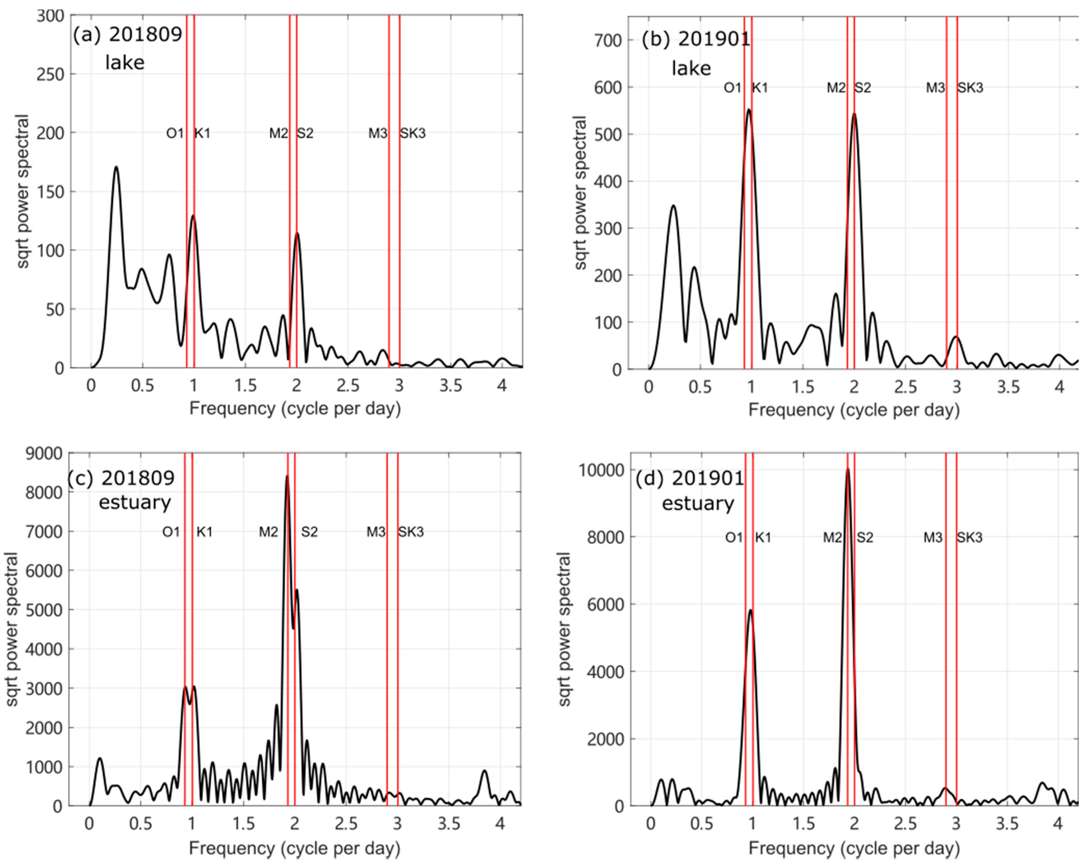
A fast Fourier transform is applied to the barometric-pressure-adjusted water level records in the lake to specify the dominant frequencies of the periodical fluctuation (Figure 4a,b). Identifiable peaks can be seen centered at frequencies of diurnal (one cycle/day) and semi-diurnal (two cycles/day) bands, and a conspicuous peak also appears at a frequency of three cycles/day in the measurement of January 2019. The diurnal signal seems to be the combination of O1 and K1 constituents, although the accurate component cannot be distinguished since the records are too short to allow the separation of O1 and K1. The semi-diurnal peak appears to be dominated by the S2 constituent, and the peak at three cpd is likely to be the result of non-linear interaction of astronomical tides. The same calculation is also applied to the sea level records (Figure 4c,d). There are two dominant peaks in both diurnal and semi-diurnal bands for the record in September 2018, but single peaks in these two bands in January 2019. It is impossible to distinguish signals with similar periods using records shorter than 15 days, especially for semi-diurnal constituents of M2 and S2 with a period difference less than half an hour. Furthermore, the power spectral densities have a peak of 0.238 cpd, corresponding to a period of 4.2 days. The low-frequency variation during the first measurement is an order of magnitude greater than the tidal signal and is not affected by the barometric effect. Neither is the tidal signal affected by the barometric effect correction. This is reasonable because the barometric pressure variation originates from weather and thus does not include any tidal frequency.

The same work has been done to the velocity records in the first measurement and the results of zonal (blue line) and meridional (black line) velocities at 13.6 m above the bottom are shown in Figure 3b. Unlike the distinct peaks at tidal and subtidal frequencies, the spectral densities of east velocity component u (blue line) and north velocity component v (black line) include various frequency bands besides the subtidal component (4.2 days) and semidiurnal/diurnal components. This means that tidal motions in the lake are relatively weak—it is obscured by motions of non-tidal frequencies.

To further analyze the surface water level variations, we apply harmonic analyses to the water level records in the lake and in the estuary. With the results of power spectra analyses, we include four major tidal constituents: S2, K1, M2, M3 (Figure 2c,d). The dominant constituents in the lake are S2 and K1, which are responsible for over 98 percentage of the total high pass signal. The amplitudes of S2 are 1.74 (1.02) cm and 1.90 (0.91) cm for the observations of September 2018 and January 2019, respectively, with (without) the barometric effect included. The K1 tidal component is slightly smaller (1.50 cm in September and 1.37 cm in January). The amplitudes of other constituents such as M2 and M3 are around 1 mm. The harmonic analyses and low-pass filters are consistent with the original observations except for the slight deviation during the landfall of Typhoon Mangkhut. Comparing with the barometric-effect-adjusted records of water level in Figure 2c, we can see the inconsistency is mainly ascribed to the inefficiency of zero-phase digital filtering. The dominant tidal components in the estuary are M2 and K1, with amplitudes of 0.84 m and 0.33 m in September and 1.06 m and 0.59 m in January, respectively.

With the above analysis of the observational data, there are three major questions: (1) where did the tidal signal come from, (2) what caused the large subtidal water level variations, and (3) why the subtidal water level variation occurred at the same time of the landfall of the typhoon? Tide can be generated by tide potential or co-oscillation from an open boundary. It can also be generated by groundwater connection with the ocean. Since Huguangyan Lake does not have an opening to the ocean, there is no co-oscillation. Tide potential is also easily excluded because it is too shallow and small to produce such a magnitude of tidal signal. For the subtidal water level variation, the possibilities include (1) wind-driven lake oscillation; and (2) influence from outside of the lake (through an opening, which is excluded, and through groundwater connection). Since the groundwater connection is possible, we need to verify if we can evaluate the wind-driven oscillation inside the lake with the magnitude of variation shown in the data. This motivated a numerical experiment demonstrated below.

3.3. Numerical Model Experimental Results Using FVCOM

To examine the possible wind-induced seiche in the lake, a numerical model is implemented using FVCOM [19]. With this purpose in mind, we do not include the tidal potential, as it would be too small to be useful. Our focus here is only the wind-driven flow and possible oscillations in the lake and no stratification is included. There should be no major stratification effect in this system as it is a small and completely closed freshwater lake. To examine the first-order wind-driven circulation, we do not need to include baroclinicity. FVCOM has shown wide applications in solving momentum and continuity equations of the ocean hydrodynamics [19], especially for the coastal region with complicated coastline and topography. For a shallow water system without a major freshwater discharge, the motion is mainly barotropic to the first order. With this consideration, salinity and temperature changes were excluded in the simulations. We apply an idealized homogeneous wind field of 10 m/s as the surface stress to this model with actual bathymetry of the lake, and the level-2.5 (MY-2.5) turbulent closure scheme [20] modified by [21]. The readers can refer to [18] for details of FVCOM. The bottom stresses in this work are calculated by the quadratic law, which is proportional to $C_d\sqrt{u^2+v^2}\left(u,v\right)$, where $C_d$ is determined by the following equation:

$$C_d=\max \left(\frac{k^2}{\ln \left(\frac{z_{\mathrm{ab}}}{z_0}\right)},0.0025\right)$$

(1)

where $k$ is the von Karman constant (0.4); $z_0$ is the bottom roughness parameter and is set to be 0.0001 in our case.

The computational mesh includes 4029 nodes and 7827 elements. The highest horizontal resolution is about 7 m. The time step of the computation is 1/6 s. Since the lake is a closed system, there is no open boundary. Wind provides the surface stress as the only forcing in this experiment. The first five days are used to ramp up the model. The wind stress is then applied. First, a constant easterly wind is applied for five days, followed by a switch of wind to the westerly for another five days, and southerly for five days, and finally northerly for five days. The magnitude of wind is always a constant of 10 m/s.

The resulting flow field is determined by wind direction, bathymetry, and coastline. The flow field in shallow water tends to be in the direction of wind but modified by the coastline and depth gradient, while the deeper water tends to have counter wind flows, especially at the bottom. These wind-driven circulations are consistent with previous studies [22,23,24].

To examine the possibility of wind-induced seiche (natural oscillation in the lake), two positions on the east (21°8.8′ N, 110°17.3′ E) and west coasts (21°8.8′ N, 110°16.4′ E) are selected from the model for analyzing the water level variations (the locations are marked with blue circle in Figure 1). The water level difference between the east and west locations is shown (Figure 5) to have an order of magnitude of only a fraction of a millimeter. Over a time of about 205.58 min, there are 38 full periods of waves, which leads to a period T₀~324.6 s (5.41 min). Along the two positions of ~L = 1645 m, we extract 20 water depth values from the FVCOM model mesh, which yields an averaged depth of h_m = 10.49 m. The theoretical value of the seiche period is thus

$$T_1=\frac{2L}{\sqrt{g{h}_m}}=325.7\sec$$

(2)

which is very close to the value ($T_0$ = 324.6 s) from the model. Therefore, there is indeed a seiche in this system, which is verified by the model results. However, the seiche is at least two to three orders of magnitude smaller than the water level variation (~0.3 m) observed in the lake. With the clear tidal signal in surface water level records, there must be groundwater connection through a pressure balance between the lake and the coastal ocean, although there should be no material exchange because the lake water is fresh.

4. Discussion

With the cautious inspection and appropriate analyses of surface water level records, we have demonstrated that the water level in the Huguangyan Lake revealed clear periodical signals of diurnal and semi-diurnal periods with amplitudes of roughly 2 cm. In view of the results from the data analysis and numerical model experiments, it is clear that a tidal signal from the water level data is unquestionable. The magnitude of tide is too large to be caused by local tidal potential: the local tidal potential would not cause a measurable or meaningful tidal signal in such a small and shallow enclosed water body. This can be seen by referring to the previous studies—the 227 m Lake Loch Ness with much larger dimensions only has a tidal amplitude of 1.5 mm [10]. Since the lake is enclosed, there is no co-oscillating tide either.

The tidal signal shown in the spectrum of Huguangyan Lake’s water level variations suggests that there may be groundwater connection between the coastal ocean and the lake. By taking out the barometric effect on the water level, and demonstrating that there is still a tidal signal, it shows that the semi-diurnal and diurnal tides cannot be produced by the air pressure variation, especially considering the fact that these tidal signals were persistent in both surveys. If there is no connection between the lake and the coastal ocean, there would be no barometric effect. Furthermore, the spectrum without the barometric correction also showed tidal signals with similar magnitude. The dominant tidal constituents in the lake are principal solar semidiurnal S2 and lunisolar diurnal K1, while those in the nearby estuary are principal lunar semidiurnal M2, solar semidiurnal S2, and diurnal K1. To distinguish two tidal constituents with similar frequencies ν₁ and ν₂, the length of hourly records N should meet the condition $\left|{\nu }_1-{\nu }_2\right|\ge {\nu }_{\mathrm{c}}/N$, where ν_c is the critical frequency of harmonic analysis and its minimum is 0.5 cycle per hour. The minimal record length should be longer than 15 days for both semidiurnal and diurnal signals, which unfortunately are not satisfied in this work. Moreover, there is no channel connection between the lake and the estuary since the lake is surrounded by solid lateral boundaries. The only possible connection of the lake to the coastal area is through porewater pressure, which may act as a filter for the frequencies of the coastal tidal signals when transmitted to the lake through nonlinear porewater dynamics.

Furthermore, the water level variation exceeded 30 cm during the passage of Typhoon Mangkhut. It is impossible for an isolated lake to experience such a significant drop and rebound of surface water level. This oscillation cannot be due to lake-wide oscillation or seiche caused by wind. As demonstrated, wind-induced seiche in the system is too small and too fast—the period is on the order of minutes, while the observed subtidal oscillation is over a much longer time period of ~4 days; and the magnitude (0.3 m) is much larger than the wind-induced seiche, which is less than a millimeter with persistent strong winds of 10 m/s.

It therefore only has one mechanism left for the lake water level oscillations—the motion is forced by a groundwater connection with the coastal ocean through porewater media. In future studies, a groundwater model should be included to quantify the tidal and storm surge signals dynamically.

The air-pressure-adjusted water level shows very different behavior before and after the typhoon. The is because the water level variation is very small and the barometric effect is relatively large. In a coastal ocean environment where tide-induced water level variation is significant, the barometric effect is barely visible because tidal range is significantly larger than the barometric pressure effect. It is also noticed that the amplitude of tidal signals inside the lake does not have a linear relationship with the tidal signal measured in the estuary (and thus coastal ocean). The interpretation is that the connection between the ocean and lake is apparently through very limited groundwater connection: otherwise, it would have larger amplitude inside the lake. Most likely, there is very limited water seepage through the porewater media and thus the connection is highly nonlinear under a certain threshold. When the forcing is over the threshold, more water can go through and cause the storm surge inside the lake during a tropical cyclone. This is verified by the variation of storm surge corresponding to the passage of Typhoon Mangkhut. Given this situation, a cross-spectrum (not presented) does not give a clear relationship because the process is highly nonlinear due to the complication of groundwater dynamics. The current study is to demonstrate for the first time that there appears to be a very limited groundwater connection that generates a small tidal signal in the closed lake that is more significant during a tropical cyclone passage. It should be noted also that this is not a storm surge problem. The Typhoon-Mangkhut-induced sea level change inside the lake is negligible, as the wind-stress does not produce any significant water level setup as demonstrated because the lake is very small. The significant water level variation shown is not created by the wind but must be by the groundwater connection to the coastal ocean. The reason that we use idealized wind in the FVCOM experiments is exactly to show that seiche is way too small to generate any significant water level variations. The surge by a direct wind forcing on the lake is simply negligible and is not of any interest to study. The storm surge in the estuary and coastal ocean acting through the groundwater apparently causes the significant water level variations and the simulation of the measured water level change cannot be accomplished without a groundwater model.

5. Summary and Conclusions

Intrigued by abnormal water level variations with apparent tidal variations in an enclosed small freshwater Huguangyan Lake, we launched a study with observations and numerical experiments. The water level variations show a mixed tidal signal (a few cm in amplitude), with both semi-diurnal and diurnal tidal constituents of comparable magnitudes. These are, however, much larger than what the local tidal potential can allow because the lake is too shallow and too small to have measurable tide generated by tide-generating force or from the Earth’s tides. The barometric effect was shown unable to generate such signals either. The time series of subtidal variation happened to have encompassed the time of Typhoon Mangkhut, which made its landfall in a nearby coast. The large subtidal variation of water level during Typhoon Mangkhut was apparently caused by the passing typhoon, which is supported by the exact timing match. The numerical model experiments allow us to exclude the lake-wide seiche caused by local wind-stress.

In summary, our study establishes the argument by excluding (1) tidal-potential effect inside the lake; (2) the wind-driven seiche; and (3) the barometric effect. The only possibility left to explain the lake oscillation as observed is a groundwater connection. This is corroborated by the correspondence of typhoon passage and the great drop in water level at around its landfall time. Therefore, the conclusion is that both the tidal and subtidal water level variations are generated through a connection with the coastal ocean through the groundwater. In other words, these are tidal and storm surge signals from the coastal ocean, not through a direct and free water exchange, but through a limited groundwater connection. This is the first such study showing that tidal signal and storm surge signal exist in the Huguangyan Lake system, with corroborating hydrodynamic evidence using a combination of methods including observations and numerical experiments.

References

- Wu, X.; Shen, J. Paleoenvironment evolution since the Holocene reflected by diffuse reflectance spectroscopy from Huguangyan Maar Lake sediments, Guangdong Province. J. Lake Sci. 2012, 24, 943–951, (In Chinese with English abstract). [Google Scholar] [CrossRef] [Green Version]
- Liu, J. Volcanoes in China; Science Press of China: Beijing, China, 1999. [Google Scholar]
- Wu, X.; Zhang, Z.; Xu, X.; Shen, J. Asian summer monsoonal variations during the Holocene revealed by Huguangyan maar lake sediment record. Palaeogeogr. Palaeoclimatol. Palaeoecol. 2012, 323, 13–21. [Google Scholar] [CrossRef]
- Liu, J.; Lü, H.; Negendank, J.; Mingram, J.; Luo, X.; Wang, W.; Chu, G. Periodicity of holocene climatic variations in the Huguangyan Maar Lake. Chin. Sci. Bull. 2000, 45, 1712–1717. [Google Scholar] [CrossRef]
- Wang, W.; Liu, J.; Liu, D.; Peng, P.; Lu, H.; Gu, Z.; Chu, G.; Negendank, J.; Luo, X.; Mingram, J. The two-step monsoon changes of the last deglaciation recorded in tropical Maar Lake Huguangyan, southern China. Chin. Sci. Bull. 2000, 45, 1529–1532. [Google Scholar] [CrossRef]
- Fuhrmann, A.; Mingram, J.; Lücke, A.; Lu, H.; Horsfield, B.; Liu, J.; Wilkes, H. Variations in organic matter composition in sediments from Lake Huguang Maar (Huguangyan), south China during the last 68 ka: Implications for environmental and climatic change. Org. Geochem. 2003, 34, 1497–1515. [Google Scholar] [CrossRef]
- Mingram, J.; Schettler, G.; Nowaczyk, N.; Luo, X.; Lu, H.; Liu, J.; Negendank, J. The Huguang maar lake-a high-resolution record of palaeoenvironmental and palaeoclimatic changes over the last 78,000 years from South China. Quatern. Int. 2004, 122, 85–107. [Google Scholar] [CrossRef]
- Wang, L.; Li, J.; Xie, L.; Chen, F.; Wang, L.; Shi, Y.; Zheng, M. Analysis of hydrological characteristics for Huguangyan Maar lake with cruise data in winter and spring. J. Guangdong Ocean Univ. 2018, 38, 63–72, (In Chinese with English abstract). [Google Scholar] [CrossRef]
- Hamblin, P.F.; Mühleisen, R.; Bösenberg, U. The astronomical tides of Lake Constance. Dtsch. Hydrogr. Z. 1977, 30, 105–116. [Google Scholar] [CrossRef]
- Pugh, D.T.; Woodworth, P.L.; Bos, M.S. Lunar tides in Loch Ness, Scotland. J. Geophys. Res. 2011, 116, 1–8. [Google Scholar] [CrossRef] [Green Version]
- Mortimer, C.H.; Fee, E.J. Free surface oscillations and Tides of lakes michigan and superior. Philos. Trans. R. Soc. A Math. Phys. Eng. Sci. 1976, 281, 1–61. [Google Scholar] [CrossRef]
- Sanchez, B.V.; Rao, D.B.; Wolfson, P.G. Objective analysis for tides in a closed basin. Mar. Geod. 1985, 9, 71–91. [Google Scholar] [CrossRef]
- Hamblin, P.F. A Theory of Short Period Tides in a Rotating Basin. Philos. Trans. R. Soc. A Math. Phys. Eng. Sci. 1976, 281, 97–111. [Google Scholar] [CrossRef]
- Hamblin, P.F. On the free surface oscillations of Lake Ontario. Limnol. Oceanog. 1982, 27, 1039–1049. [Google Scholar] [CrossRef]
- Platzman, G.W. The daily variation of water level on Lake Erie. J. Geophys. Res. 1966, 71, 2471–2483. [Google Scholar] [CrossRef]
- Trebitz, A.S. Characterizing seiche and tide-driven daily water level fluctuations affecting coastal ecosystems of the Great Lakes. J. Great Lakes Res. 2006, 32, 102–116. [Google Scholar] [CrossRef]
- Taylor, B.N.; Thompson, A. The International System of Units (SI); NIST Special Publication 330 2008; NOAA: Gaithersburg, MD, USA, 2019; pp. 1–92. [Google Scholar]
- Emery, W.J.; Thomson, R.E. Data Analysis Methods in Physical Oceanography, 2nd ed.; Elsevier Science: New York, NY, USA, 2004; 654p. [Google Scholar] [CrossRef]
- Chen, C.S.; Liu, H.D.; Beardsley, R. An unstructured grid, finite-volume, three-dimensional, primitive equations ocean model: Application to coastal ocean and estuaries. J. Atmos. Ocean. Technol. 2003, 20, 159–186. [Google Scholar] [CrossRef]
- Mellor, G.; Yamada, T. Development of a turbulence closure model for geophysical fluid problems. Rev. Geophys. 1982, 20, 851–875. [Google Scholar] [CrossRef] [Green Version]
- Galperin, B.; Kantha, L.; Hassid, S.; Rosati, A. A quasi-equilibrium turbulent energy model for geophysical flows. J. Atmos. Sci. 1988, 45, 55–62. [Google Scholar] [CrossRef] [Green Version]
- Engelund, F. Steady wind set-up in prismatic lakes. In Environmental Hydraulics: Stratified Flows, Lecture Notes on Coastal and Estuarine Studies; Pedersen, F.B., Ed.; Springer: New York, NY, USA, 1986; Volume 18, pp. 205–212. [Google Scholar] [CrossRef]
- Li, C.; Huang, W.; Chen, C.; Lin, H. Flow regimes and adjustment to wind-driven motions in lake Pontchartrain Estuary: A modeling experiment using FVCOM. J. Geophys. Res. Oceans 2018, 123, 8460–8488. [Google Scholar] [CrossRef]
- Huang, W.; Li, C. Spatial variation of cold front wind-driven circulation and quasi-steady state balance in lake Pontchartrain Estuary. Estuar. Coast Shelf Sci. 2019, 224, 154–170. [Google Scholar] [CrossRef]