


1. Introduction
Deterministic motion of a colloidal-scale species can be induced by the concentration gradient of a surrounding solute. For charged colloids in electrolyte solutions, the concentration gradient of the electrolyte causes motion known as diffusiophoresis (Anderson Reference Anderson1989; Velegol et al. Reference Velegol, Garg, Guha, Kar and Kumar2016; Marbach & Bocquet Reference Marbach and Bocquet2019). Diffusiophoresis is an electrokinetic phenomenon, comprising a chemiphoretic component due to the osmotic pressure gradient developed along the colloid surface, and an electrophoretic component due to the junction potential generated by the diffusion of ions with different diffusivities. Prieve et al. (Reference Prieve, Anderson, Ebel and Lowell1984) derived the drift velocity of a diffusiophoretic colloid,  $\boldsymbol {u} = M \boldsymbol {\nabla } \log S$, which was confirmed experimentally (Staffeld & Quinn Reference Staffeld and Quinn1989; Abecassis et al. Reference Abecassis, Cottin-Bizonne, Ybert, Ajdari and Bocquet2008; Palacci et al. Reference Palacci, Abecassis, Cottin-Bizonne, Ybert and Bocquet2010, Reference Palacci, Cottin-Bizonne, Ybert and Bocquet2012; Kar et al. Reference Kar, Chiang, Rivera, Sen and Velegol2015; Banerjee et al. Reference Banerjee, Williams, Azevedo, Helgeson and Squires2016; Shi et al. Reference Shi, Nery-Azevedo, Abdel-Fattah and Squires2016; Shin et al. Reference Shin, Um, Sabass, Ault, Rahimi, Warren and Stone2016; Ault et al. Reference Ault, Warren, Shin and Stone2017; Shin et al. Reference Shin, Ault, Warren and Stone2017; Ault, Shin & Stone Reference Ault, Shin and Stone2018). The diffusiophoretic velocity relates to the gradient of the logarithm of the solute concentration
  $S$ via the diffusiophoretic mobility
  $M$, which has been termed a ‘log-sensing’ response (Palacci et al. Reference Palacci, Cottin-Bizonne, Ybert and Bocquet2012). The mobility encompasses information about the colloid and the solute, including the colloid surface potential and ionic diffusivities. A positive and a negative
  $M$ correspond to the colloids driven up and down the solute gradient, respectively. Since the solute concentration in a system is often inhomogeneous, diffusiophoresis plays a role in numerous natural phenomena and applications such as mineral replacement reactions, drug delivery and enhanced oil recovery (Velegol et al. Reference Velegol, Garg, Guha, Kar and Kumar2016; Marbach & Bocquet Reference Marbach and Bocquet2019).
While diffusiophoresis is a physico-chemical phenomenon, perhaps surprisingly it shares the same log-sensing relation with a biological phenomenon: chemotaxis (Keller & Segel Reference Keller and Segel1971; Brown & Berg Reference Brown and Berg1974; Kalinin et al. Reference Kalinin, Jiang, Tu and Wu2009; Marbach & Bocquet Reference Marbach and Bocquet2019). Chemotaxis refers to microorganisms utilizing their transmembrane chemoreceptors to detect the surrounding solute gradient, along which they perform deterministic motion (Engelmann Reference Engelmann1881; Adler Reference Adler1966; Brown & Berg Reference Brown and Berg1974; Parkinson & Kofoid Reference Parkinson and Kofoid1992; Eisenbach et al. Reference Eisenbach, Lengeler, Varon, Gutnick, Meili, Firtel, Segall, Omann, Tamada and Murakami2004; Wadhams & Armitage Reference Wadhams and Armitage2004). A widely studied example is Escherichia coli. In an inhomogeneous solute field, the bacteria sense the solute gradient in a temporal fashion and use that information to modulate the probability of their run-and-tumble events. Runs are extended in favourable directions, resulting in a net movement of the bacteria up/down the gradient of the solute (attractant/repellent) (Brown & Berg Reference Brown and Berg1974; Wu et al. Reference Wu, Roberts, Kim, Koch and DeLisa2006). Chemotaxis is central to phenomena such as biofilm formation (Eisenbach et al. Reference Eisenbach, Lengeler, Varon, Gutnick, Meili, Firtel, Segall, Omann, Tamada and Murakami2004) and has been utilized in bioremediation including aquifer restoration (Ford & Harvey Reference Ford and Harvey2007; Adadevoh et al. Reference Adadevoh, Ostvar, Wood and Ford2017). In chemotactic log-sensing,  $M$ is the chemotactic sensitivity. Velocity relations other than log-sensing have been proposed to capture various hallmarks of chemotaxis in more general regimes (Lapidus & Schiller Reference Lapidus and Schiller1976; Segel Reference Segel1977; Rivero et al. Reference Rivero, Tranquillo, Buettner and Lauffenburger1989; Tindall et al. Reference Tindall, Porter, Maini, Gaglia and Armitage2008; Menolascina et al. Reference Menolascina, Rusconi, Fernandez, Smriga, Aminzare, Sontag and Stocker2017; Salek et al. Reference Salek, Carrara, Fernandez, Guasto and Stocker2019). Recent studies also suggest that diffusiophoresis could contribute to the movement of living colloidal species in addition to chemotaxis (Marbach & Bocquet Reference Marbach and Bocquet2019; Sear Reference Sear2019).
To model the spatio-temporal evolution of a population of chemotactic/diffusiophoretic colloidal species (which we will refer to as ‘colloids’ in the rest of this article, for brevity), one must solve the coupled solute and colloid advection–diffusion–reaction equations (Lapidus & Schiller Reference Lapidus and Schiller1976; Rivero-Hudec & Lauffenburger Reference Rivero-Hudec and Lauffenburger1986; Staffeld & Quinn Reference Staffeld and Quinn1989; Ford & Cummings Reference Ford and Cummings1992; Marx & Aitken Reference Marx and Aitken2000; Abecassis et al. Reference Abecassis, Cottin-Bizonne, Ybert, Ajdari and Bocquet2008; Tindall et al. Reference Tindall, Porter, Maini, Gaglia and Armitage2008; Palacci et al. Reference Palacci, Abecassis, Cottin-Bizonne, Ybert and Bocquet2010, Reference Palacci, Cottin-Bizonne, Ybert and Bocquet2012; Kar et al. Reference Kar, Chiang, Rivera, Sen and Velegol2015; Banerjee et al. Reference Banerjee, Williams, Azevedo, Helgeson and Squires2016; Shi et al. Reference Shi, Nery-Azevedo, Abdel-Fattah and Squires2016; Shin et al. Reference Shin, Um, Sabass, Ault, Rahimi, Warren and Stone2016; Ault et al. Reference Ault, Warren, Shin and Stone2017, Reference Ault, Shin and Stone2018; Shin et al. Reference Shin, Ault, Warren and Stone2017; Raynal et al. Reference Raynal, Bourgoin, Cottin-Bizonne, Ybert and Volk2018; Raynal & Volk Reference Raynal and Volk2019; Shim, Stone & Ford Reference Shim, Stone and Ford2019; Chu et al. Reference Chu, Garoff, Tilton and Khair2020a). The evolving solute gradient induces a chemical-driven chemotactic/diffusiophoretic drift velocity which contributes to the advective flux of the colloids, in addition to that due to any imposed hydrodynamic flow,  $\boldsymbol {v}$, such as blood flows in diffusiophoretic colloidal drug delivery and interstitial fluid flows in chemotactic bioremediation of aquifers. Reactions of colloids refer to an increase (source) or decrease (sink) in the total amount of the colloids, e.g. death of bacteria (Servais, Billen & Rego Reference Servais, Billen and Rego1985; Golding et al. Reference Golding, Kozlovsky, Cohen and Ben-Jacob1998; Tindall et al. Reference Tindall, Porter, Maini, Gaglia and Armitage2008). In general, chemotactic/diffusiophoretic colloid transport occurs in two or higher spatial dimensions, for example, in a microchannel. Predicting the transport via direct numerical simulations is costly especially at long times, since the shortest time scale where the transport occurs has to be resolved. For instance, for chemotaxis/diffusiophoresis in a hydrodynamic flow in a long thin channel of radius
  $R$, where the colloid diffusivity
  $D_c$ is typically smaller or comparable to the solute diffusivity
  $D_s$ (Ford & Lauffenburger Reference Ford and Lauffenburger1991; Lewus & Ford Reference Lewus and Ford2001; Tindall et al. Reference Tindall, Porter, Maini, Gaglia and Armitage2008; Cussler Reference Cussler2009; Shin et al. Reference Shin, Um, Sabass, Ault, Rahimi, Warren and Stone2016; Shim et al. Reference Shim, Stone and Ford2019), the shortest transport time scale is the solute radial diffusion time
  $R^2/D_s$. This is much smaller than the solute(colloid) convective time
  $L/\bar {v}$ along the length of the channel
  $L$ (
$L$ ( $v$ is the axial component of
  $\boldsymbol {v}$ and overbar denotes a cross-sectional average). Nevertheless, one can leverage this separation of time scales to construct asymptotic schemes to predict the solute and colloid transport.
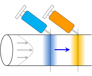
To illustrate the idea, let us first focus on the solute transport in the absence of colloids, as shown in figure 1. The hydrodynamic flow induces concentration gradients of the solute in the radial direction for times shorter than  $R^2/D_s$. However, diffusion acts to smooth these gradients. At times longer than
  $R^2/D_s$, where the solute has fully sampled the velocity variations across the cross-section of the channel, its concentration no longer varies in the radial direction: only axial gradients persist. Hence, the transport becomes one-dimensional. Taylor (Reference Taylor1953) originally made this brilliant physical observation and subsequently proposed and experimentally verified that the two-dimensional transport equation for the solute concentration can be reduced to a one-dimensional ‘macrotransport’ equation for the cross-sectional averaged solute concentration. Specifically, the averaged concentration field translates with the mean speed of the hydrodynamic flow and undergoes an enhanced axial diffusion, or Taylor dispersion (Aris Reference Aris1956; Brenner & Edwards Reference Brenner and Edwards1993), due to the coupling between axial convection and radial diffusion.

Figure 1. Illustration of Taylor hydrodynamic dispersion.
In this work, we follow Taylor's approach (Taylor Reference Taylor1953) to derive a macrotransport equation for a chemotactic/diffusiophoretic colloidal species under hydrodynamic flows and transient solute gradients. A key idea is that, because radial solute gradients are homogenized at long times, chemical-driven chemotactic/diffusiophoretic fluxes in the radial direction can be ignored in the colloid macrotransport. Axial solute gradients and thus chemical-driven fluxes in the axial direction may still be present, however, and they are captured in the colloid macrotransport. The rest of this article is outlined as follows. In § 2, we formulate the problem by deriving a macrotransport (averaged) equation for the two-dimensional, advection–diffusion–reaction transport of a chemotactic/diffusiophoretic colloidal species in a uniform, circular channel. We define three flow regimes, from weak to strong hydrodynamic flow strength, where the macrotransport equation is applicable. In § 3, we verify the macrotransport equation by comparing its predicted colloid transport with that from direct numerical simulation of the two-dimensional equation. Comparisons are conducted for all three aforementioned flow regimes as well as for a non-unity colloid-to-solute diffusivity ratio, suitable for modelling chemotaxis and diffusiophoresis. The implementation of the macrotransport equation to a non-circular channel and non-log-sensing models of chemical-driven transport is also elucidated. In § 4, we summarize this study and offer ideas for future work.
2. Diffusiophoretic chemotactic macrotransport model
2.1. Mathematical formulation
We consider diffusiophoresis/chemotaxis of a colloidal species due to a surrounding solute gradient in an incompressible, unidirectional hydrodynamic flow  $v$ inside a uniform, circular channel of radius
  $R$ (figure 2). The channel wall is impenetrable to the solute and the colloid. The steady hydrodynamic flow
  $v(r)$ is directed along the axial direction
  $z$ and may vary in the radial direction
  $r$. The colloid
  $C(r,z,t)$ and solute
  $S(r,z,t)$ concentration fields are symmetrically distributed about the channel centreline, and may vary in the radial and axial directions, and in time
  $t$. For
  $C \ll S$, which is common for colloidal or bacterial suspensions containing molecular solutes, the influence of the evolution of
  $C$ on
  $S$ is negligible (Lapidus & Schiller Reference Lapidus and Schiller1976; Rivero-Hudec & Lauffenburger Reference Rivero-Hudec and Lauffenburger1986; Staffeld & Quinn Reference Staffeld and Quinn1989; Ford & Cummings Reference Ford and Cummings1992; Marx & Aitken Reference Marx and Aitken2000; Abecassis et al. Reference Abecassis, Cottin-Bizonne, Ybert, Ajdari and Bocquet2008; Tindall et al. Reference Tindall, Porter, Maini, Gaglia and Armitage2008; Palacci et al. Reference Palacci, Abecassis, Cottin-Bizonne, Ybert and Bocquet2010, Reference Palacci, Cottin-Bizonne, Ybert and Bocquet2012; Kar et al. Reference Kar, Chiang, Rivera, Sen and Velegol2015; Banerjee et al. Reference Banerjee, Williams, Azevedo, Helgeson and Squires2016; Shi et al. Reference Shi, Nery-Azevedo, Abdel-Fattah and Squires2016; Shin et al. Reference Shin, Um, Sabass, Ault, Rahimi, Warren and Stone2016; Ault et al. Reference Ault, Warren, Shin and Stone2017, Reference Ault, Shin and Stone2018; Peraud et al. Reference Peraud, Nonaka, Bell, Donev and Garcia2017; Shin et al. Reference Shin, Ault, Warren and Stone2017; Balu & Khair Reference Balu and Khair2018; Raynal et al. Reference Raynal, Bourgoin, Cottin-Bizonne, Ybert and Volk2018; Raynal & Volk Reference Raynal and Volk2019; Shim et al. Reference Shim, Stone and Ford2019; Chu et al. Reference Chu, Garoff, Tilton and Khair2020a). The advection–diffusion transport of the solute is governed by
 \begin{equation} \frac{\partial S}{\partial t} + v \frac{\partial S}{\partial z} = \frac{D_s}{r}\frac{\partial}{\partial r}\left( r\frac{\partial S}{\partial r} \right) + D_s \frac{\partial^2 S}{\partial z^2}, \end{equation}
where  $D_s$ is the constant, intrinsic solute diffusivity. The hydrodynamic flow causes solute concentration gradients in the radial direction for
  $t < R^2/D_s$. However, diffusion acts to smooth these gradients. Following Taylor's and Aris’ (Aris Reference Aris1956) analyses, subsequent studies (Bailey & Gogarty Reference Bailey and Gogarty1962; Gill & Sankarasubramanian Reference Gill and Sankarasubramanian1970; Ng & Rudraiah Reference Ng and Rudraiah2008) showed that, at times larger than the solute radial diffusive time
  $t \geq R^2/D_s$, variations in the solute concentration across the channel cross-section have been smeared out, and the macrotransport equation for the cross-sectional averaged solute concentration,
  $\bar {S}(z,t)$, is
 \begin{equation} \frac{\partial \bar{S}}{\partial t} + \bar{v} \frac{\partial \bar{S}}{\partial z} = \left( D_s + \frac{\bar{v}^2 R^2}{48D_s} \right) \frac{\partial^2 \bar{S}}{\partial z^2} \quad \text{for} \ t \geq R^2/D_s, \end{equation}
where the cross-sectional average is  $\bar {(\cdot )} = \int ^{2{\rm \pi} }_0 \int ^R_0 (\cdot ) r\, \textrm {d} r \, \textrm {d}\theta / {\rm \pi}R^2$ with
  $\theta$ being the azimuth, and the second term in the bracket is an enhanced axial diffusion, or Taylor dispersion (Taylor Reference Taylor1953; Aris Reference Aris1956; Brenner & Edwards Reference Brenner and Edwards1993), owing to the coupling between axial convection and radial diffusion.

Figure 2. A diffusiophoretic/chemotactic colloidal species in a solute gradient inside a uniform, circular channel of radius  $R$ under an incompressible, unidirectional hydrodynamic flow
  $v$. The solute gradient induces a chemical-driven flow
  $\boldsymbol {u}$ of the colloids via diffusiophoresis/chemotaxis, where the colloids can be attracted (as shown) or repelled.
The evolving solute gradient induces a chemical-driven flow  $\boldsymbol {u}(S)$ of the diffusiophoretic/chemotactic colloids. The solute gradient also induces a slip flow adjacent to the channel walls, known as diffusioosmosis. However, the effect of diffusioosmosis on the solute and colloid transport is negligible to the leading order of the aspect ratio of the channel (Ault et al. Reference Ault, Shin and Stone2018) and thus it is ignored in the present study. As discussed in § 1, an important feature in common between diffusiophoresis and chemotaxis is the log-sensing chemical flow response,
  $\boldsymbol {u} = M \boldsymbol {\nabla } \log S$. Note, however, that the present derivation is not limited to any particular form of the chemical flow, and thus we keep the general notation
  $\boldsymbol {u}$. In contrast to the hydrodynamic flow
  $v$, the chemical flow is usually compressible (
 $\boldsymbol {\nabla } \boldsymbol {\cdot } \boldsymbol {u} \neq 0$) due to the spatio-temporal variation of the solute concentration. Under the chemical and hydrodynamic flow, the advection–diffusion–reaction equation for the diffusiophoretic/chemotactic colloids is
 \begin{equation} \frac{\partial C}{\partial t} + v \frac{\partial C}{\partial z} + \frac{1}{r} \frac{\partial (r u_r C)}{\partial r} + \frac{\partial (u_z C)}{\partial z} = \frac{D_c}{r}\frac{\partial}{\partial r}\left( r\frac{\partial C}{\partial r} \right) + D_c \frac{\partial^2 C}{\partial z^2} - \varGamma C, \end{equation}
where  $u_r(r,z,t)$ and
  $u_z(r,z,t)$ are the radial and axial components of the chemical flow, respectively. In diffusiophoresis,
  $D_c$ is the constant, intrinsic diffusivity of the colloid (Staffeld & Quinn Reference Staffeld and Quinn1989; Abecassis et al. Reference Abecassis, Cottin-Bizonne, Ybert, Ajdari and Bocquet2008; Palacci et al. Reference Palacci, Abecassis, Cottin-Bizonne, Ybert and Bocquet2010, Reference Palacci, Cottin-Bizonne, Ybert and Bocquet2012; Kar et al. Reference Kar, Chiang, Rivera, Sen and Velegol2015; Banerjee et al. Reference Banerjee, Williams, Azevedo, Helgeson and Squires2016; Shi et al. Reference Shi, Nery-Azevedo, Abdel-Fattah and Squires2016; Shin et al. Reference Shin, Um, Sabass, Ault, Rahimi, Warren and Stone2016; Ault et al. Reference Ault, Warren, Shin and Stone2017, Reference Ault, Shin and Stone2018; Shin et al. Reference Shin, Ault, Warren and Stone2017; Raynal et al. Reference Raynal, Bourgoin, Cottin-Bizonne, Ybert and Volk2018; Raynal & Volk Reference Raynal and Volk2019; Chu et al. Reference Chu, Garoff, Tilton and Khair2020a). In chemotaxis,
  $D_c$ is the random motility of the microorganism. Since a run of a bacterium typically last for approximately a second before being interrupted by a rapid [
 $(0.1)\ \text {s}$] tumble and subsequent change its direction (Brown & Berg Reference Brown and Berg1974; Ford & Lauffenburger Reference Ford and Lauffenburger1991; Wu et al. Reference Wu, Roberts, Kim, Koch and DeLisa2006), microorganism motility is random and can be interpreted as a diffusivity on times longer than the runtime, which is of the order of seconds. Note that such an interpretation is valid for the macrotransport equation which applies for
  $t \geq R^2/D_c$. For instance, in a typical microfluidic setting for bacteria where
  $R = 10^{-4}\ \text {m}$ and
  $D_c = 10^{-9}\ \text {m}^2\ \text {s}^{-1}$,
  $R^2/D_c = 10\ \text {s}$ is longer than the correlation time of the bacteria run-and-tumble motion. On a different note,
  $D_c$ may generally depend on the solute concentration and gradient. It is taken as a constant here as in many prior studies (see a comprehensive review by Tindall et al. Reference Tindall, Porter, Maini, Gaglia and Armitage2008) and was justified for a shallow spatial and temporal gradient (Ford & Lauffenburger Reference Ford and Lauffenburger1991). Regarding the reaction term
  $\varGamma C$, in chemotaxis it represents the death of microorganisms due to biological cycles or toxic environments (Servais et al. Reference Servais, Billen and Rego1985; Golding et al. Reference Golding, Kozlovsky, Cohen and Ben-Jacob1998; Tindall et al. Reference Tindall, Porter, Maini, Gaglia and Armitage2008). The decay rate
  $\varGamma$ is taken as a constant here.
Our goal is to derive an averaged, or macrotransport, equation from (2.3), suitable for probing the cross-sectionally averaged colloid concentration at long times,  $t \geq R^2/D_c$. For typical diffusiophoresis/chemotaxis systems where
  $D_c/D_s \leq 1$ (Ford & Lauffenburger Reference Ford and Lauffenburger1991; Lewus & Ford Reference Lewus and Ford2001; Tindall et al. Reference Tindall, Porter, Maini, Gaglia and Armitage2008; Cussler Reference Cussler2009; Shin et al. Reference Shin, Um, Sabass, Ault, Rahimi, Warren and Stone2016; Shim et al. Reference Shim, Stone and Ford2019), the long-time condition for the solute is automatically satisfied so long as that for the colloid is met. Recall that for
  $t \geq R^2/D_s$ radial solute gradients have been homogenized by the hydrodynamic flow. This justifies dropping the radial chemical flow
  $u_r$ in (2.3) and the axial chemical flow
  $u_z$ varies only in
  $z$. We further write the colloid concentration and the hydrodynamic flow in terms of their cross-sectional averages (overbar) and variations, or fluctuations, therefrom (prime):
  $C(r,z,t) = \bar {C}(z,t) + C'(r,z,t)$ and
  $v(r) = \bar {v} + v'(r)$. Equation (2.3) becomes
 \begin{align} &\frac{\partial (\bar{C} + C')}{\partial t} + (\bar{v} + v') \frac{\partial (\bar{C} + C')}{\partial z} + \frac{\partial (\bar{u}_z \bar{C})}{\partial z} = \frac{D_c}{r}\frac{\partial}{\partial r}\left( r\frac{\partial C'}{\partial r} \right) \nonumber\\ &\quad + D_c \frac{\partial^2 (\bar{C} + C')}{\partial z^2} - \varGamma (\bar{C} + C'). \end{align}
The cross-sectional average of (2.4) is
 \begin{equation} \frac{\partial
\bar{C}}{\partial t} + \bar{v} \frac{\partial
\bar{C}}{\partial z} + \overline{v' \frac{\partial C'}{\partial
z}} + \frac{\partial (\bar{u}_z \bar{C})}{\partial z} = D_c
\frac{\partial^2 \bar{C}}{\partial z^2} - \varGamma
\bar{C}. \end{equation}
\begin{equation} \frac{\partial
\bar{C}}{\partial t} + \bar{v} \frac{\partial
\bar{C}}{\partial z} + \overline{v' \frac{\partial C'}{\partial
z}} + \frac{\partial (\bar{u}_z \bar{C})}{\partial z} = D_c
\frac{\partial^2 \bar{C}}{\partial z^2} - \varGamma
\bar{C}. \end{equation}
To solve for  $C'$, we subtract (2.5) from (2.4) and invoke two assumptions following Taylor's classical analysis (Taylor Reference Taylor1953; Aris Reference Aris1956; Brenner & Edwards Reference Brenner and Edwards1993): namely, (i)
  $C' \ll \bar {C}$, and (ii) the contribution to the colloid transport by the axial diffusion is small relative to the radial diffusion at long times,
  $t \geq R^2/D_c$. The governing equation of
  $C'$ is thus obtained as
 \begin{equation} v' \frac{\partial \bar{C}}{\partial z} = \frac{D_c}{r}\frac{\partial}{\partial r}\left( r\frac{\partial C'}{\partial r} \right) - \varGamma C'. \end{equation}
Valdes-Parada et al. (Reference Valdes-Parada, Porter, Narayanaswamy, Ford and Wood2009) presented a similar equation to (2.6) in the development of a macrotransport theory for non-decaying ( $\varGamma = 0$) chemotactic bacteria. In their equation, there is an additional term associated with ‘chemotactic dispersion’, that is, the enhancement or reduction of the axial diffusion of colloids due to the radial solute gradient. However, above, we have justified that such an effect can be ignored for
  $t \geq R^2/D_s$.
Subramanian & Gill (Reference Subramanian and Gill1974), who studied the dispersion of a decaying species in the absence of chemical flows, pointed out that (2.6) should not be used to determine the dispersion due to species decay, as was erroneously done by others (Gupta & Gupta Reference Gupta and Gupta1972; Vidyanidhi & Murty Reference Vidyanidhi and Murty1976). They conducted a separate analysis, showing exactly that the effect of species decay only manifests in the  $\varGamma \bar {C}$ term in (2.5) without any additional dispersion. In other words,
  $\varGamma C'$ can be dropped from (2.6). The resulting equation can be integrated twice to obtain an expression for
  $C'$ which, upon multiplying with
  $v'$ and averaging the product, gives
 \begin{equation} \overline{v'C'} ={-}D_{c,Dis} \frac{\partial \bar{C}}{\partial z}, \end{equation}
where the dispersivity of the colloid is defined as
 \begin{equation} D_{c,Dis} ={-}\frac{2}{R^2} \int^R_0 \left[ \frac{v'}{D_c} \int^r_0 \frac{1}{r_1} \left( \int^R_{r_1} v'(r_2) r_2 \, \textrm{d} r_2 \right) \, \textrm{d} r_1 \right] r\, \textrm{d} r, \end{equation}
in which  $r_1$ and
  $r_2$ are dummy variables. The dispersivity
  $D_{c,Dis}$ can be determined for a given hydrodynamic flow
  $v$. In the present case for a steady, pressure-driven laminar flow in a uniform circular tube, we recover Taylor's result
  $D_{c,Dis}= \bar {v}^2 R^2 / 48 D_c$ (Taylor Reference Taylor1953) for
  $v(r) = -{\rm \Delta} P R^2 (1 - r^2/R^2)/4\eta$,
  $\bar {v} = -{\rm \Delta} P R^2/8\eta$,
  $v'(r) = -{\rm \Delta} P R^2 (1/2 - r^2/R^2)/4\eta$, where
  ${\rm \Delta} P$ is the applied pressure gradient and
  $\eta$ is the solvent viscosity. On recognizing that
  $\partial (\overline {v'C'}) / \partial z = \overline {v' \partial C' / \partial z}$, (2.7) gives
 \begin{equation} \overline{v' \frac{\partial C'}{\partial z}} ={-}D_{c,Dis} \frac{\partial^2 \bar{C}}{\partial z^2}. \end{equation}
Upon substituting (2.9) into (2.5), finally we obtain
 \begin{equation} \frac{\partial \bar{C}}{\partial t} + \bar{v} \frac{\partial \bar{C}}{\partial z} + \frac{\partial (\bar{u}_z \bar{C})}{\partial z} = \left( D_c + \frac{\bar{v}^2 R^2}{48D_c} \right) \frac{\partial^2 \bar{C}}{\partial z^2} - \varGamma \bar{C} \quad \text{for} \ t \geq R^2/D_c. \end{equation}
Equation (2.10) is a key result of this work: it represents a macrotransport equation for a diffusiophoretic/chemotactic colloidal species under a hydrodynamic flow and evolving solute gradient. Hydrodynamic flow contributes to dispersion via the dispersivity  $D_{c,Dis}$, the second term in the bracket on the right-hand side of (2.10). We reiterate that by dispersion we mean the enhanced axial diffusion due to the coupling of axial convection and radial diffusion. Thus, chemical flow does not cause dispersion at long times but it does contribute to colloid advection and spreading, i.e. macrotransport, via the term
  $\partial (\bar {u}_z \bar {C}) / \partial z$. This term is in turn influenced by the action of the hydrodynamic flow on the solute gradient.
Equation (2.10) reduces to classical macrotransport equations in limiting cases. For instance, when there is no solute gradient,  $\partial (\bar {u}_z \bar {C}) / \partial z$ vanishes and (2.10) recovers the result of Subramanian & Gill (Reference Subramanian and Gill1974), where colloid diffusion is solely governed by the sum of the colloid intrinsic diffusivity/motility and hydrodynamic dispersion. Further, when there is no solute gradient and the colloid is non-decaying,
  $\partial (\bar {u}_z \bar {C}) / \partial z$ and
  $\varGamma \bar {C}$ vanish, and (2.10) recovers Taylor's and Aris’ classical result (Taylor Reference Taylor1953; Aris Reference Aris1956). Equation (2.10) is valid formally for
  $t \geq R^2 / D_c$ (Bailey & Gogarty Reference Bailey and Gogarty1962; Gill & Sankarasubramanian Reference Gill and Sankarasubramanian1970; Ng & Rudraiah Reference Ng and Rudraiah2008). Thus, for most diffusiophoresis/chemotaxis systems where
  $D_c/D_s \leq 1$ (Ford & Lauffenburger Reference Ford and Lauffenburger1991; Lewus & Ford Reference Lewus and Ford2001; Tindall et al. Reference Tindall, Porter, Maini, Gaglia and Armitage2008; Cussler Reference Cussler2009; Shin et al. Reference Shin, Um, Sabass, Ault, Rahimi, Warren and Stone2016; Shim et al. Reference Shim, Stone and Ford2019), (2.10) is applicable for
  $t \geq R^2 / D_c \geq R^2 / D_s$, whereas for cases where
  $D_c/D_s \geq 1$, (2.10) is applicable for
  $t \geq R^2 / D_s \geq R^2 / D_c$. A typical value of
  $R^2/D_c = 10 \text {s}$ for chemotaxis is noted in the previous paragraph; for diffusiophoresis,
  $R = 10^{-5}\text {m}$ and
  $D_c \leq 10^{-11} \text {m}^2\text {s}^{-1}$,
  $R^2/D_c \geq 10 \text {s}$ is the regime of major interest in common diffusiophoretic systems (Shin et al. Reference Shin, Um, Sabass, Ault, Rahimi, Warren and Stone2016). We remark that (2.10) is general to any initial distributions of the solute and the colloid, such as a Gaussian or a spike. In § 3.5, we will discuss the generalization of (2.10) to other models of the chemical flow and channels of arbitrary but uniform cross-sections.
2.2. Hydrodynamic flow regimes of macrotransport
Probstein (Reference Probstein2003) characterized three different hydrodynamic flow regimes of the original Taylor–Aris solute macrotransport equation. To prepare for testing the present macrotransport theory in these regimes in the next section, below we recapitulate Probstein's analysis and extend it to the present colloidal species macrotransport.
To facilitate the discussion, the original Taylor–Aris solute macrotransport (2.2) is normalized using the following scales,
 \begin{equation} \left.
\begin{gathered}\displaystyle \hat{t} = \dfrac{t}{R^2/D_s},
\quad \hat{r} = \dfrac{r}{R}, \quad \hat{z} = \dfrac{z}{L},
\quad \hat{u}_z = \dfrac{u_z}{\bar{v}}, \quad \hat{u}_r =
\dfrac{u_r}{\bar{v}} \dfrac{L}{R},\\ \displaystyle
\hat{\varGamma} = \dfrac{\varGamma}{D_s/R^2}, \quad \hat{C}
= \dfrac{C}{C_0}, \quad \hat{S} = \dfrac{S}{S_0}, \quad
\epsilon = \dfrac{R}{L}, \quad Pe = \dfrac{\bar{v}R}{D_s},
\end{gathered} \right\} \end{equation}
\begin{equation} \left.
\begin{gathered}\displaystyle \hat{t} = \dfrac{t}{R^2/D_s},
\quad \hat{r} = \dfrac{r}{R}, \quad \hat{z} = \dfrac{z}{L},
\quad \hat{u}_z = \dfrac{u_z}{\bar{v}}, \quad \hat{u}_r =
\dfrac{u_r}{\bar{v}} \dfrac{L}{R},\\ \displaystyle
\hat{\varGamma} = \dfrac{\varGamma}{D_s/R^2}, \quad \hat{C}
= \dfrac{C}{C_0}, \quad \hat{S} = \dfrac{S}{S_0}, \quad
\epsilon = \dfrac{R}{L}, \quad Pe = \dfrac{\bar{v}R}{D_s},
\end{gathered} \right\} \end{equation}
where  $L$ and
  $\epsilon < 1$ is the length and aspect ratio of the channel, respectively;
  $C_0$ and
  $S_0$ are the characteristic colloid and solute concentration; and
  $Pe$ is the Péclet number which describes the relative importance of hydrodynamic convection of solute to solute intrinsic diffusivity. The normalized solute macrotransport equation reads
 \begin{equation} \frac{\partial \hat{\bar{S}}}{\partial \hat{t}} + \epsilon Pe \frac{\partial \hat{\bar{S}}}{\partial \hat{z}} = \left( \epsilon^2 + \epsilon^2 \frac{Pe^2}{48} \right) \frac{\partial^2 \hat{\bar{S}}}{\partial \hat{z}^2}. \end{equation}
The first regime defined by Probstein is the Taylor regime, where convection dominates dispersion ( $\epsilon Pe \gg \epsilon ^2 Pe^2 / 48$) and dispersion dominates intrinsic diffusion (
 $\epsilon ^2 Pe^2 / 48 \gg \epsilon ^2$). This sets the range of
  $Pe$ as
  $48/\epsilon \gg Pe \gg \sqrt {48}$. The second one is the convective axial diffusion regime, the opposite limit to the Taylor regime, where convection dominates intrinsic diffusion (
 $\epsilon Pe \gg \epsilon ^2$) and the latter dominates dispersion (
 $\epsilon ^2 \gg \epsilon ^2 Pe^2 / 48$). This gives
  $48/\epsilon \gg Pe \ll \sqrt {48}$. In between the Taylor and the convective axial diffusion regimes is the Taylor–Aris regime where convection dominates dispersion (
 $\epsilon Pe \gg \epsilon ^2 Pe^2 / 48$) while dispersion is comparable to intrinsic diffusion (
 $\epsilon ^2 Pe^2 / 48 \sim \epsilon ^2$). This gives
  $Pe$ as
  $48/\epsilon \gg Pe$ and
  $Pe$ should be between
  $Pe \gg \sqrt {48}$ and
  $Pe \ll \sqrt {48}$. For example,
  $\epsilon = 5 \times 10^{-4}$ and
  $Pe = 10$ would satisfy these conditions for the Taylor–Aris regime.
Here, we extend Probstein's analysis to the present colloid macrotransport (2.10). The normalized colloid macrotransport equation reads,
 \begin{equation} \frac{\partial \hat{\bar{C}}}{\partial \hat{t}} + \epsilon Pe \frac{\partial \hat{\bar{C}}}{\partial \hat{z}} + \epsilon Pe \frac{\partial (\hat{\bar{u}}_z \hat{\bar{C}})}{\partial \hat{z}} = \left( \epsilon^2 \frac{D_c}{D_s} + \epsilon^2 \frac{D_s}{D_c} \frac{Pe^2}{48} \right) \frac{\partial^2 \hat{\bar{C}}}{\partial \hat{z}^2} - \hat{\varGamma} \hat{\bar{C}}. \end{equation}
The range of  $Pe$ for each regime is obtained as follows. Convective axial diffusion regime:
  $(48/\epsilon )(D_c/D_s) \gg Pe \ll (D_c/D_s)\sqrt {48}$; Taylor–Aris regime:
  $(48/\epsilon )(D_c/D_s) \gg Pe$ for
  $Pe$ between
  $Pe \gg (D_c/D_s)\sqrt {48}$ and
  $Pe \ll (D_c/D_s) \sqrt {48}$; Taylor regime:
  $(48/\epsilon )(D_c/D_s) \gg Pe \gg (D_c/D_s)\sqrt {48}$. Since the colloid macrotransport requires coupling to the solute macrotransport, their conditions for
  $Pe$ have to be considered together. Focusing on
  $D_c/D_s \leq 1$, this sets the following conditions for the present macrotransport framework:
 \begin{equation} \left.\begin{gathered}
\displaystyle \text{Convective axial diffusion} :
\dfrac{48}{\epsilon} \dfrac{D_c}{D_s} \gg Pe \ll
\dfrac{D_c}{D_s}\sqrt{48},\\ \displaystyle
\text{Taylor-Aris} : \dfrac{48}{\epsilon} \dfrac{D_c}{D_s}
\gg Pe, \text{ between } Pe \gg \sqrt{48} \text{ and } Pe
\ll \dfrac{D_c}{D_s}\sqrt{48},\\ \displaystyle
\text{Taylor} : \dfrac{48}{\epsilon} \dfrac{D_c}{D_s} \gg
Pe \gg \sqrt{48}. \end{gathered} \right\}
\end{equation}
\begin{equation} \left.\begin{gathered}
\displaystyle \text{Convective axial diffusion} :
\dfrac{48}{\epsilon} \dfrac{D_c}{D_s} \gg Pe \ll
\dfrac{D_c}{D_s}\sqrt{48},\\ \displaystyle
\text{Taylor-Aris} : \dfrac{48}{\epsilon} \dfrac{D_c}{D_s}
\gg Pe, \text{ between } Pe \gg \sqrt{48} \text{ and } Pe
\ll \dfrac{D_c}{D_s}\sqrt{48},\\ \displaystyle
\text{Taylor} : \dfrac{48}{\epsilon} \dfrac{D_c}{D_s} \gg
Pe \gg \sqrt{48}. \end{gathered} \right\}
\end{equation}
The convective axial diffusion, Taylor–Aris and Taylor regime can be interpreted as weak, intermediate and strong hydrodynamic flow regimes, respectively. In the next section, we compare the colloid transport in these regimes predicted from the macrotransport equations ((2.2) and (2.10)) with that from direct numerical simulation of the two-dimensional transport equations ((2.1) and (2.3)).
3. Results and discussion
In this section, we test the present macrotransport theory ((2.2) and (2.10)) by comparing its prediction with that from direct numerical simulation of the two-dimensional transport equations ((2.1) and (2.3)). We solve the macrotransport and the two-dimensional equations using the ‘Coefficient Form PDE’ and the time-dependent, implicit ‘backward differentiation formula (BDF) solver’ in COMSOL. The equations are discretized with free triangular (for two-dimensional equations) and uniform (for macrotransport equations) elements with a maximum size  $5 \times 10^{-3} L$. Adaptive time stepping is selected to capture the flow dynamics on the fast, radial diffusive time scale. Convergence of solutions are acquired with a relative tolerance
  $\delta = 10^{-4}$ between successive solutions. Zero-concentration boundary conditions are set at the channel inlet,
  $z = 0$, and outlet,
  $z = L$, for both the solute and colloids. In all comparisons below, both solute and colloidal species are sufficiently far away from the inlet and outlet over the course of their time evolution, mimicking an infinitely long channel. Because of the different strengths of hydrodynamic flow examined, different initial locations of the solute and colloid centroid are used across §§ 3.1–3.4. The log-sensing relation is used to model the chemical flow. A small background solute concentration
  $S_b = 10^{-3} {max}[S(t=0)]$ is imposed to prevent the unphysically large velocity as
  $S \rightarrow 0$, that is we write
  $\boldsymbol {u} = M \boldsymbol {\nabla } \log (S + S_b)$. We have tested that, as long as the same
  $S_b$ is used between the macrotransport theory and the direct numerical simulation of the two-dimensional transport equations, it does not alter the excellent agreements between the two sets of results that we will show in §§ 3.1–3.4. We focus our analyses on a non-decaying colloidal species,
  $\varGamma = 0$; readers are referred to e.g. Subramanian & Gill (Reference Subramanian and Gill1974); Shapiro & Brenner (Reference Shapiro and Brenner1986) for detailed discussions of the dispersion of decaying colloids. The averaged solute and colloid concentrations from the two-dimensional equations are obtained from cross-sectionally averaging the (two-dimensional) concentration fields upon solving the equations. In §§ 3.1–3.3, we consider
  $D_c/D_s = 1$, which is typical for chemotaxis (Ford & Lauffenburger Reference Ford and Lauffenburger1991; Lewus & Ford Reference Lewus and Ford2001; Tindall et al. Reference Tindall, Porter, Maini, Gaglia and Armitage2008; Shim et al. Reference Shim, Stone and Ford2019). In § 3.4, we consider
  $D_c/D_s < 1$, which is general to probe diffusiophoresis (Cussler Reference Cussler2009; Shin et al. Reference Shin, Um, Sabass, Ault, Rahimi, Warren and Stone2016). In § 3.5, we discuss the generality of the macrotransport theory to non-log-sensing chemical flows and non-circular channels.
3.1. Convective axial diffusion regime: weak hydrodynamic flow
By observing (2.14), for  $D_c/D_s = 1$ we choose
  $\epsilon = 5 \times 10^{-3}$ and
  $Pe = 1$ to compute the solute and colloidal species transport in the convective axial diffusion regime. Figure 3 shows the time evolution of the normalized averaged solute and colloid concentration profiles. Dotted lines correspond to results obtained from the macrotransport theory, whereas solid lines are from the two-dimensional transport equations. The initial conditions are the same between two sets of results, namely
  $S/(Q_s/L)|_{\hat {t}=0} = {\exp [-(\hat {z}/\hat {f} - \hat {z}_s/\hat {f})^2]}/(\hat {f}\sqrt {{\rm \pi} })$ and
  $C/(Q_c/L)|_{\hat {t}=0} = {\exp [-(\hat {z}/\hat {g} - \hat {z}_c/\hat {g})^2]}/(\hat {g}\sqrt {{\rm \pi} })$, where
  $Q_s$ and
  $Q_c$ are the solute and colloid mass per unit cross-sectional area of the channel, respectively (arbitrary here);
  $\hat {f} = f/L = 0.05$ and
  $\hat {g} = g/L = 0.025$ control the initial width of the solute and colloid distribution, respectively; and
  $\hat {z}_s = z_s/L = 0.2$ and
  $\hat {z}_c = z_c/L = 0.1$ are the initial location of the solute and colloid centroid, respectively. Since the colloid evolution depends on the solute dynamics, let us first examine figure 3(a). At times longer than the solute radial diffusive time, there is an excellent agreement in the predictions between the macrotransport and the two-dimensional equations. The agreement is supported and quantified by the small difference in the centroid
  ${\rm \Delta} \mu _s$ (and variance
  ${\rm \Delta} \sigma ^2_s$) between the two sets of results, where
  ${\rm \Delta} \mu _s \equiv |(\int ^1_0 z\bar {S} \, \textrm {d} z / \int ^1_0 \bar {S} \, \textrm {d} z)_{{macro}} - (\int ^1_0 z\bar {S} \, \textrm {d} z / \int ^1_0 \bar {S} \, \textrm {d} z)_{{2D}}|$ and
  ${\rm \Delta} \sigma ^2_s \equiv |( \int ^1_0 z^2\bar {S} \, \textrm {d} z / \int ^1_0 \bar {S} \, \textrm {d} z) - \mu ^2_s )_{{macro}} - ( \int ^1_0 z^2\bar {S} \, \textrm {d} z / \int ^1_0 \bar {S} \, \textrm {d} z) - \mu ^2_s )_{{2D}} |$ (Aris Reference Aris1956; Chu et al. Reference Chu, Garoff, Tilton and Khair2020a). The difference in the centroid of the colloid distribution
  ${\rm \Delta} \mu _c$ (and variance
  ${\rm \Delta} \sigma ^2_c$) between the macrotransport and two-dimensional equations, which will be used in figure 3(b,c) and following figures, share a similar definition but with
  $\bar {S}$ in the integrals replaced by
  $\bar {C}$.

Figure 3. Time evolution of the normalized averaged (a) solute  $\bar {S}/(Q_s/L)$ and (b,c) colloidal species
  $\bar {C}/(Q_c/L)$ concentration profiles for
  $D_c/D_s = 1$,
  $\epsilon = 5 \times 10^{-3}$ and
  $Pe = 1$. In (b),
  $M/D_s = 5$; in (c),
  $M/D_s = 25$. Dotted lines: macrotransport theory, (2.2) and (2.10); solid lines: two-dimensional transport equations, (2.1) and (2.3).
As the solute distribution evolves in time, so does the solute concentration gradient. This induces a chemical flow of the colloidal species. The evolutions of the colloid concentration profile are shown in figure 3(b,c) for  $M/D_s = 5$ and
  $M/D_s = 25$, respectively. These values are typical for chemotaxis (Ford & Lauffenburger Reference Ford and Lauffenburger1991; Tindall et al. Reference Tindall, Porter, Maini, Gaglia and Armitage2008) where a larger positive
  $M/D_s$ represents a stronger attraction between the solute and the colloid. Such a large
  $M/D_s$ is rare in diffusiophoresis but is potentially attainable in some physico-chemical systems, such as near a liquid–liquid demixing critical point (Sear & Warren Reference Sear and Warren2017; Ault et al. Reference Ault, Shin and Stone2018; Chu et al. Reference Chu, Garoff, Tilton and Khair2020a). Let us first inspect figure 3(b). We see an excellent agreement between the two sets of results [an equally good agreement is also obtained for
  $t/(R^2/D_s) = 1$ but it is not shown here for clarity]. Specifically, by comparing figure 3(a,b), colloids are attracted towards the solute. Initially, the separation distance between the solute and colloid centroids is
  $0.1$. After
  $50$ radial diffusive times, the two centroids coincide. Thus, chemical flow causes a significant colloid movement when hydrodynamic flow is weak and the macrotransport theory captures this attraction response. In fact, a scaling criterion can be obtained from the normalized colloid macrotransport (2.10), which determines when chemical flow is comparable to the hydrodynamic flow,
 \begin{equation} \epsilon Pe \approx \epsilon^2 \frac{M}{D_s} \frac{1}{\hat{f}}. \end{equation}
The factor  $1/\hat {f}$ arises from the axial length of the solute gradient although the strength of a log-sensing chemical flow is independent of the solute concentration by recognizing that
  $\partial (\log S) / \partial z = (\partial S / \partial z) / S$. In this case, the strength of the chemical flow, the right-hand side of (3.1), is comparable to the hydrodynamic flow, the left-hand side of the equation.
Figure 4 shows the (two-dimensional) normalized concentration profiles of the solute and colloidal species obtained from the two-dimensional transport equations for figure 3(a,b). Since the concentration profiles are axisymmetric about the centreline of the channel, only half of the profile is shown in each contour plot with the top face of the plot corresponding to the centreline of the channel. Hydrodynamic flow is from left to right. In figure 4, from  $\hat {t} = t / (R^2/D_s) = 0$ to
  $\hat {t} = 10$, the initial solute and colloid distributions are deformed and they follow the parabolic hydrodynamic flow profile. The parabolic profile is more obvious in the colloidal species due to its narrower initial distribution. At
  $\hat {t} = 10$, there is a slight radial non-uniformity in
  $C$. This is a consequence of the hydrodynamic flow and the non-uniform solute attraction owing to the axially varying solute concentration gradient. Note how the colloid profile spans over different concentration (colour) gradients of the solute distribution. However, the effect of such a slight non-uniformity is insignificant to the macrotransport description, since the predictions of the macrotransport and the two-dimensional equation agree well (figure 3b). Meanwhile, the colloids are attracted towards the solute with time. As noted in the previous paragraph, the centroids of the solute and the colloid coincide at
  $\hat {t} = 50$.


Next, let us look at figure 3(c), where  $M/D_s = 25$ and it shares the same solute evolution figure 3(a) with figure 3(b). In this case, the colloids are attracted towards the solute much faster compared to figure 3(b), as expected. Contraction of the colloid profile is also more prominent. The macrotransport and the two-dimensional equations are in good agreement. The slight deviation between the two sets of prediction is due to numerical artifacts of mass ‘leakage’ – a consequence of the propagation of discretization errors in solving the convection-dominated transport equation, which is numerically unstable (Ferziger & Peric Reference Ferziger and Peric2002). These discretization errors are physically irrelevant and increase with the dimension of the system. This highlights the advantage of using the (one-dimensional) macrotransport equation as opposed to direct numerical simulation. Further, the computational runtime for the macrotransport equation is at least
  $O(10^3)$ times shorter than the two-dimensional equation.
The macrotransport equation also captures repelling chemical-driven transport, i.e.  $M<0$, as shown in figure 5. The solute and colloid initial conditions are the same as before, except that
  $\hat {z}_c = 0.3$. On comparing figure 5(b,c), the translation of the colloid downstream with chemical-driven repulsion (figure 5c) is more significant than that without chemical flow figure 5(b). In figure 5(c), the asymmetry of the colloid distribution is due to the fact that, for a Gaussian solute distribution, the log-sensing chemical flow is linearly proportional to the distance from the peak of the solute distribution (Chu et al. Reference Chu, Garoff, Tilton and Khair2020a). Thus, in log-sensing chemotaxis/diffusiophoresis, a Gaussian solute distribution induces a spatially non-uniform velocity to the colloid distribution and thus gives rise to an asymmetric distribution. The asymmetry in colloid distribution is not apparent in the attractant case (figure 3) because the colloid distribution is contracted and the non-uniformity in chemical flow is present over a narrow profile only. In contrast, the asymmetric in colloid distribution is more prominent in the repellent case (figure 5c) because the colloid distribution is broadened and there is a large non-uniformity of chemical flow velocity over the wide profile.

Figure 5. Time evolution of the normalized averaged (a) solute  $\bar {S}/(Q_s/L)$ and (b-c) colloidal species
  $\bar {C}/(Q_c/L)$ concentration profiles for
  $D_c/D_s = 1$,
  $\epsilon = 5 \times 10^{-3}$, and
  $Pe = 1$. In (b),
  $M/D_s = 0$; in (c),
  $M/D_s = -1$. Dotted lines: macrotransport theory, (2.2) and (2.10); solid lines: two-dimensional transport equations, (2.1) and (2.3).
Beyond the above validation, we remark that the convective axial diffusion regime is a quasi-one-dimensional regime of macrotransport that we had implicitly assumed in our previous study of spreading of diffusiophoretic colloids due to transient solute gradients (Chu et al. Reference Chu, Garoff, Tilton and Khair2020a). Specifically, the colloids translate with the mean speed of the hydrodynamic flow. Colloid spreading, or macrotransport, is solely governed by the chemical flow and the intrinsic colloid diffusion, while spreading enhancement due to hydrodynamic dispersion is negligible. In other words, our previous study has to observe the rather tight constraint on  $Pe$ set by (2.14) for the convective axial diffusion regime. Otherwise, for larger
  $Pe$, the hydrodynamic dispersivity becomes comparable to or larger than the intrinsic diffusivity. Then, ignoring dispersivity would yield significant errors, particularly in the variance of the colloid profile.
3.2. Taylor–Aris regime: intermediately strong hydrodynamic flow
In this section, we analyse the performance of the macrotransport theory ((2.2) and (2.10)) in capturing the two-dimensional transport ((2.1) and (2.3)) in the Taylor–Aris regime, where the solute/colloid intrinsic diffusivity is comparable to the corresponding hydrodynamic dispersivity. By observing (2.14), we choose  $\epsilon = 5 \times 10^{-4}$ and
  $Pe = 10$. The solute and colloid initial conditions are the same as figure 3. As shown in figure 6, the agreements between the two sets of results are excellent. Distinct from the comparisons in § 3.1, here the separation between the solute and colloid centroids remain the same over time. This can be understood by referring to the scaling criterion (3.1), where in this case the chemical flow is much weaker than the hydrodynamic flow. Thus, reduction in the separation between the solute and the colloid centroids, which is proportional to the strength of the chemical flow, is negligible compared to the translation due to the hydrodynamic flow.

Figure 6. Time evolution of the normalized averaged (a) solute  $\bar {S}/(Q_s/L)$ and (b) colloidal species
  $\bar {C}/(Q_c/L)$ concentration profiles for
  $D_c/D_s = 1$,
  $\epsilon = 5 \times 10^{-4}$,
  $Pe = 10$ and
  $M/D_s = 1$. Dotted lines: macrotransport theory, (2.2) and (2.10); solid lines: two-dimensional transport equations, (2.1) and (2.3).
3.3. Taylor regime: strong hydrodynamic flow
In this section, we check the performance of the macrotransport theory in the Taylor regime, where the solute/colloid hydrodynamic dispersivity dominates the corresponding intrinsic diffusivity. From (2.14), we choose  $\epsilon = 5 \times 10^{-5}$ and
  $Pe = 100$. The solute and colloid initial conditions are the same as figure 3. Figure 7 shows that the predictions of the macrotransport theory agree well with those by the two-dimensional transport equations. As in the Taylor–Aris regime, here the separation between the solute and colloid centroids remain the same over time, since the hydrodynamic flow dominates the chemical flow. In particular, the colloid evolution is essentially identical for
  $M/D_s = 0$ and
  $M/D_s = 1$. The implication of this observation is that under a strong hydrodynamic flow the solute and colloid equations could be treated as if they were uncoupled. Thus, even though the colloids are chemotactic, their transport due to the solute gradient is negligible.

Figure 7. Time evolution of the normalized averaged (a) solute  $\bar {S}/(Q_s/L)$ and (b-c) colloidal species
  $\bar {C}/(Q_c/L)$ concentration profiles for
  $D_c/D_s = 1$,
  $\epsilon = 5 \times 10^{-5}$ and
  $Pe = 100$. In (b),
  $M/D_s = 0$; in (c),
  $M/D_s = 1$. Dotted lines: macrotransport theory, (2.2) and (2.10); solid lines: two-dimensional transport equations, (2.1) and (2.3).
3.4. Systems with non-unity diffusivity ratio $D_c/D_s$

In this section, we test the applicability of the macrotransport theory to diffusiophoresis. Distinct from chemotaxis, the ratio of the colloidal species to solute diffusivity in typical diffusiophoresis settings is much smaller than unity,  $D_c/D_s \leq O(10^{-2})$. As a result, probing colloid transport at long times compared to the radial diffusion time scale (where the macrotransport theory applies) demands computing the solute and colloid dynamics for over hundreds of solute radial diffusive times, which is extremely costly. Worse still, the discretization errors, which grow in time and are especially significant in solving the two-dimensional equations, will contaminate the long-time solution and affect the comparison as conducted in the previous sections.
Thus, to show that the macrotransport theory applies to diffusiophoresis and generally for  $D_c/D_s \neq 1$, we perform the comparison for
  $D_c/D_s = 0.1$, as shown in figure 8. We conduct the analysis in the convective axial diffusion regime, since we showed that in this regime the effect of the chemical flow is comparable to the hydrodynamic flow. From (2.14), we choose
  $\epsilon = 5 \times 10^{-3}$ and
  $Pe = 0.1$. For typical diffusiophoresis,
  $|M/D_s| \leq 1$ (Prieve et al. Reference Prieve, Anderson, Ebel and Lowell1984; Shin et al. Reference Shin, Um, Sabass, Ault, Rahimi, Warren and Stone2016) and we choose
  $M/D_s = 1$. The solute and colloid initial conditions are the same as before, except that
  $\hat {z}_s = 0.4$ and
  $\hat {z}_c = 0.3$. As in the comparisons in the previous sections, the predictions by the macrotransport equations agree very well with those by the two-dimensional transport equations. Substantial attraction of the colloids to the solute is also observed, as expected in the convective axial diffusion regime.

Figure 8. Time evolution of the normalized averaged (a) solute  $\bar {S}/(Q_s/L)$ and (b) colloidal species
  $\bar {C}/(Q_c/L)$ concentration profiles for
  $D_c/D_s = 0.1$,
  $\epsilon = 5 \times 10^{-3}$,
  $Pe = 0.1$ and
  $M/D_s = 1$. Dotted lines: macrotransport theory, (2.2) and (2.10); solid lines: two-dimensional transport equations, (2.1) and (2.3).
3.5. Generality of macrotransport to other chemical flows and channel geometries
In this section, we show how the macrotransport theory can be generalized to channels of other cross-sections and to incorporate non-log-sensing chemical flows. Recall that the macrotransport theory ((2.2), (2.10) and (2.14)) is derived for a uniform circular tube. However, the same macrotransport equations can be applied to channels of other cross-sections by simply replacing the dispersion coefficient  $48$ by a different coefficient for another channel geometry. For instance, one could easily repeat the averaging procedure in § 2 for a pressure-driven flow in a parallel-plate channel and arrive at the same macrotransport equation, with a dispersion coefficient
  $210$ (Wooding Reference Wooding1960) and the channel radius
  $R$ replaced by the channel height
  $h$. Dispersion coefficients for other cross-sections have been derived, for example concentric/eccentric cylinders as a model for cerebrospinal fluid flows within a spinal cavity (Sankarasubramanian & Gill Reference Sankarasubramanian and Gill1971; Chu et al. Reference Chu, Garoff, Tilton and Khair2020b), non-ideal microchannels with bowing (Dutta, Ramachandran & Leighton Reference Dutta, Ramachandran and Leighton2006), and channels with slowly varying cross-sections or micropatterns (Bryden & Brenner Reference Bryden and Brenner1996; Chu et al. Reference Chu, Garoff, Przybycien, Tilton and Khair2019).
The macrotransport theory is also general to incorporate arbitrary forms of chemical flows. As shown in § 2.1, derivations of the macrotransport equation did not assume any particular form of the chemical flow. While the log-sensing relation is standard to model diffusiophoresis, this relation is just a first approximation to chemotaxis. For example, it does not account for the shear-induced reorientation of chemotactic bacteria, which has been shown to significantly impact bacterial concentration profiles (Rusconi, Guasto & Stocker Reference Rusconi, Guasto and Stocker2014; Bearon & Hazel Reference Bearon and Hazel2015; Secchi et al. Reference Secchi, Vitale, Mino, Kantsler, Eberl, Rusconi and Stocker2020). Chemotactic flow models have been derived in this regard, e.g. (Bearon & Pedley Reference Bearon and Pedley2000), and can be incorporated in the macrotransport theory. Other chemotactic velocity relations have been proposed. For instance, Lapidus & Schiller (Reference Lapidus and Schiller1976) introduced the receptor-ligand dissociation constant of the microorganism in their proposed velocity relation, which gives a better agreement with the experiments by Dahlquist, Lovely & Koshland (Reference Dahlquist, Lovely and Koshland1972) and Mesibov, Ordal & Adler (Reference Mesibov, Ordal and Adler1973). Rivero et al. (Reference Rivero, Tranquillo, Buettner and Lauffenburger1989) proposed a velocity relation for describing the population-level microorganism transport based on individual microscopic variables, such as the single-cell swim speed, persistence time and temporal receptor occupation. More recently, Menolascina et al. (Reference Menolascina, Rusconi, Fernandez, Smriga, Aminzare, Sontag and Stocker2017) and Salek et al. (Reference Salek, Carrara, Fernandez, Guasto and Stocker2019) proposed a finite-range log-sensing model, which captures a hallmark of chemotaxis that microorganism log-sensing occurs only above a threshold solute concentration. Thus, the generality of the macrotransport theory to account for arbitrary forms of chemical flows will enable analysis of more biologically realistic models of chemotaxis.
4. Conclusions
In this work, we have derived a macrotransport equation for predicting the long-time chemotactic/diffusiophoretic colloidal species transport in a uniform circular tube in which there is a transient solute gradient and the hydrodynamic flow is uniaxial and steady. We have compared the predictions obtained from the macrotransport equation with that from the original, two-dimensional transport equation. The comparisons are conducted in three regimes where classical macrotransport theory applies: convective axial diffusion (weak hydrodynamic flow); Taylor–Aris (intermediately strong hydrodynamic flow); and Taylor (strong hydrodynamic flow) regime. In all three regimes, we have obtained excellent agreements between the macrotransport and two-dimensional equations. Discretization errors, which increase with the dimension of the problem, are mitigated in the reduced-order macrotransport model and the computational runtime for solving the macrotransport model is in general  $O(10^3)$ times shorter than numerical solution of the two-dimensional advection–diffusion–reaction equation. We have identified that, in the convective axial diffusion regime, hydrodynamic dispersion is negligible compared to intrinsic diffusion. Thus, the evolution of the cross-sectionally averaged colloid concentration can be described by the macrotransport equation where colloid spreading is solely due to the chemical flow and the intrinsic colloid diffusion. In addition, we have presented a scaling criterion for determining when a chemical flow would cause significant colloid transport amid a hydrodynamic flow. We have also discussed how the macrotransport equation can be generalized for channels of arbitrary cross-section as well as to incorporate other forms of chemical flows necessary for capturing recently revealed hallmarks of chemotaxis.
For future work, the macrotransport theory can be employed to examine in more detail the interplay between chemical and hydrodynamic flows on colloid transport. A few relevant studies exist (Yan, Bouwer & Hilpert Reference Yan, Bouwer and Hilpert2014; Yan & Hilpert Reference Yan and Hilpert2014) although their scopes are restricted due to the high computational cost associated with fully resolving the two-/three-dimensional solute and colloid transport. The present theory can be leveraged to efficiently explore the large parameter space involved in a system with hydrodynamic and chemical flows, particularly comparing predictions with different velocity models proposed for chemotaxis. For instance, in the macrotransport model an exact solution can be obtained for deposition of a point source of colloid in a Gaussian distribution of solute, which we will describe in detail in future work. This seemingly idealized example is in fact applicable to examine the long-time colloid transport with arbitrary forms of initial distribution, since any distribution asymptotes to a Gaussian at long times (Bender & Orszag Reference Bender and Orszag1999; Chu et al. Reference Chu, Garoff, Tilton and Khair2020a).
Acknowledgements
H.C.W.C. acknowledges the assistance of T.-L. Hsieh in setting up the COMSOL simulations.
Funding
This work was partly funded by Procter  $\&$ Gamble. H.C.W.C. also acknowledges the startup funding support from the Division of Sponsored Programs, Department of Chemical Engineering, and Herbert Wertheim College of Engineering at University of Florida.
Declaration of interest
The authors report no conflict of interest.


 Open access