Outliers in Semi-Parametric Estimation of Treatment Effects

Abstract

Outliers can be particularly hard to detect, creating bias and inconsistency in the semi-parametric estimates. In this paper, we use Monte Carlo simulations to demonstrate that semi-parametric methods, such as matching, are biased in the presence of outliers. Bad and good leverage point outliers are considered. Bias arises in the case of bad leverage points because they completely change the distribution of the metrics used to define counterfactuals; good leverage points, on the other hand, increase the chance of breaking the common support condition and distort the balance of the covariates, which may push practitioners to misspecify the propensity score or the distance measures. We provide some clues to identify and correct for the effects of outliers following a reweighting strategy in the spirit of the Stahel-Donoho (SD) multivariate estimator of scale and location, and the S-estimator of multivariate location (Smultiv). An application of this strategy to experimental data is also implemented.

1. Introduction

Treatment effect techniques are the workhorse tool when examining the causal effects of interventions, i.e., whether the outcome for an observation is affected by the participation in a program or policy (treatment). As Bassi (1983, 1984); Hausman and Wise (1985) argue, counterfactual estimates are precise when using randomized experiments; yet, when looking at non-randomized experiments, there are a number of assumptions, such as unconfoundedness, exogeneity, ignorability, or selection on observables, that should be considered before estimating the true effect, or to get close to that of a randomized experiment Imbens (2004)1.

While the above assumptions are usually considered when identifying treatment effects (see King et al. (2017)), one that has been overlooked in the existing literature is the existence of outliers (on both the outcome and the covariates).2 A number of issues arise from the existence of outliers, for example these may bias or modify estimates of priority interest, and in our case, the treatment effect (see some discussion in Rasmussen (1988); Schwager and Margolin (1982); and Zimmerman (1994)); they may also increase the variance and reduce the power of methods, especially those within the non-parametric family. If non-randomly distributed, they may reduce normality, violating in the multivariate analyses the assumption of sphericity and multivariate normality, as noted by Osborne and Overbay (2004).

To the best of our knowledge, the effects of outliers on the estimation of semi-parametric treatment effects have not yet been analyzed in the literature. The only reference is Imbens (2004), who directly associates outlying values in the covariates to a lack of overlap. Imbens (2004) argues that outlier observations will present estimates of the probability of receiving treatment close to 0 or 1, and therefore methods dealing with limited overlap can produce estimates approximately unchanged in bias and precision. As shown in this paper, this intuition is valid only for outliers that are considered good leverage points. Moreover, Imbens (2004) argues that treated observations with outlying values may lead to biased covariate matching estimates, because these observations would be matched to inappropriate controls. Control observations with outlying covariate values, on the other hand, will likely have little effect on the estimates of average treatment effect for the treated, since such observations are unlikely to be used as matches. We provide evidence for this intuition.

Thus, in this paper, we examine the relative performance of semi-parametric estimators of average treatment effects in the presence of outliers. Three types of outliers are considered: bad leverage points, good leverage points, and vertical outliers. The analysis considers outliers located in the treatment group, the control group, and in both groups. We focus on (i) the effect of these outliers in the estimates of the metric, propensity score, and Mahalanobis distance; (ii) the effect of those metrics contaminated by outliers in the matching procedure when finding counterfactuals; and (iii) the effect of these matches on the estimates of the average treatment effect on the treated (TOT).

Using Monte Carlo simulations, we show that the semi-parametric estimators of average treatment effects produce biased estimates in the presence of outliers. Our findings show that, first the presence of bad leverage points (BLP) yield a bias of the estimators of average treatment effects. The bias emerges because this type of outlier completely changes the distribution of the metrics used to define good counterfactuals, and therefore changes the matches that had initially been undertaken, assigning as matches observations with very different characteristics. This effect is independent of the location of the outlier observation. Second, good leverage points (GLP) in the treatment sample slightly bias estimates of average treatment effects, because they increase the chance of violating the overlap condition. Third, good leverage points in the control sample do not affect the estimates of treatment effects, because they are unlikely to be used as matches. Fourth, these outliers distort the balance of the covariates criterion used to specify the propensity score. Fifth, vertical outliers in the outcome variable greatly bias estimates of average treatment effects. Sixth, good leverage points can be identified visually by looking at the overlap plot. Bad leverage points, however, are masked in the estimation of the metric and are, as a consequence, practically impossible to identify unless a formal outlier identification method is implemented.

To identify outliers we suggest two strategies that are robust, one based on the Stahel (1981) and Donoho (1982) estimator of scale and location, proposed in the literature by Verardi et al. (2012) and the other proposed by Verardi and McCathie (2012). What we suggest is thus identifying all types of outliers in the data by this method and estimating treatment effects again, down-weighting the importance of outliers; this is a one-step re-weighted treatment effect estimator. Monte Carlo simulations support the utility of these tools for overcoming the effects of outliers in the semi-parametric estimation of treatment effects.

An application of these estimators to the data of LaLonde (1986) allows us to understand the failure of the matching estimators of Dehejia and Wahba (1999, 2002) to overcome LaLonde’s critique of non-experimental estimators. We show that the large bias, when considering LaLonde’s full sample, of Dehejia and Wahba (1999, 2002), which was criticized by Smith and Todd (2005) can be explained by the presence of outliers in the data. When the effect of these outliers is down-weighted, the matching estimates of Dehejia and Wahba (1999, 2002) approximate the experimental treatment effect of LaLonde’s sample.

This paper is structured as follows: Section 2 briefly reviews the literature. Section 3 defines the balancing hypothesis, the semi-parametric estimators, and the types of outliers considered, as well as the S-estimator and the Stahel-Donoho estimator of location and scatter tool to detect outliers. In Section 4, the data generating process (DGP) is characterized. The analysis of the effects of outliers is presented in Section 5. An application to LaLonde’s data is presented in Section 6, and in Section 7, we conclude.

2. A Brief Review of the Literature

Different methodologies for identifying outliers have been proposed in the literature; using statistical reasoning (Hadi et al. (2009)); distances (Angiulli and Pizzuti (2002); Knorr et al. (2000); Orair et al. (2010)), and densities (Breunig et al. (2000)); (De Vries et al. (2010); Keller et al. (2012)). However, the issue has not been completely resolved and this issue may become especially troublesome, because the problem increases as outliers often do not show up by simple visual inspection or by univariate analysis, and in the case several outliers are grouped close together in a region of the sample space, far away from the bulk of the data, they may mask one another (see Rousseeuw and Van Zomeren (1990)).

To illustrate the outliers problem, in a labor market setting such as that employed by Ashenfelter (1978) and Ashenfelter and Card (1985), consider a case in which the path of the data clearly shows that highly educated people attend a training program and uneducated individuals do not. Now assume a small number of individuals without schooling are participating in the program and a small number of educated individuals are not, while having similar remaining characteristics. Enrolled individuals with an outstanding level of education may represent good leverage points. However, both small groups mentioned above, on the other hand, may constitute bad leverage points in the treatment and control sample, respectively. Regardless of whether this small number of individuals genuinely belong to the sample or are errors from the data encoding process, they may have a large influence on the treatment effect estimates and drive the conclusion about the impact of the training program for the entire sample, as pointed out by Khandker et al. (2009) and Heckman and Vytlacil (2005). The problem considered in this paper is that as semi-parametric techniques, matching methods rely on a parametric estimation of the metrics (propensity score and Mahalanobis distance) used to define and compare observations with similar characteristics in terms of covariates, while the relationship between the outcome variables and the metric is nonparametric. Therefore, the presence of multivariate outliers in the data set can yield a strong bias of the estimators of the metrics and lead to unreliable treatment effect estimates. According to the findings of Rousseeuw and Van Zomeren (1990), vertical outliers can also bias the nonparametric relationship between the metric and the outcome by distorting the average outcome in either the observed or counterfactual group. Moreover, these distortions, caused by the presence of multivariate outliers in the data set, can distort the balance of the covariates when specifying the propensity score, as in Dehejia (2005). These issues have practical implications: when choosing the variables to specify the propensity score, it may not be necessary to discard troublesome but relevant variables from a theoretical point of view or generate senseless interactions or nonlinearities. It might be sufficient to discard troublesome observations (outliers). That is, outliers can push practitioners to unnecessarily misspecify the propensity score.

3. Framework

To examine the effects of outliers on the average treatment effect we identify ouliers and implement a correction in the spirit of Verardi et al. (2012); Stahel (1981) and Donoho (1982), and the other one in the spirit of Verardi and McCathie (2012). Next, we briefly describe the outlier classification criteria, the re-weighting methods and a description of the matching methods used.

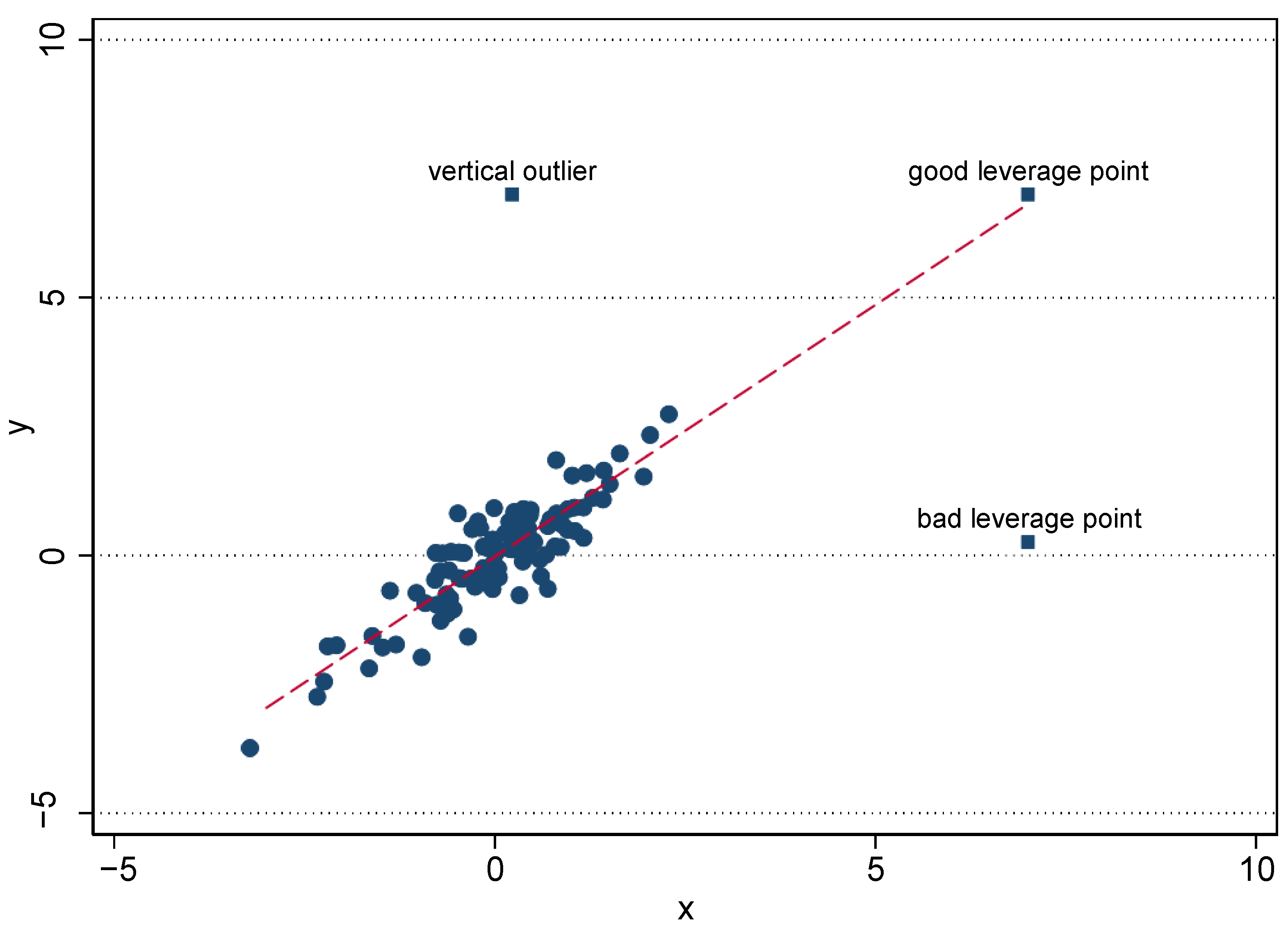
(i) Classification of outliers: Semi-parametric estimators of treatment effects may be sensitive to outliers. To understand the sources of bias caused by outliers, we employ the simple cross-section regression analysis. Rousseeuw and Leroy (2005) argue that bias may be of three kinds, the error term (vertical outliers) and the explanatory variables (good and bad leverage points) (see Figure 1). Vertical outliers (VO) are those observations that are far away from the bulk of the data in the y-dimension, but that present a behavior similar to the group in the x-dimension. In the treatment effects framework, these would be outliers on the outcomes of study. Good leverage points (GLP), on the other side, are observations that are far from the bulk of the data in the x-dimension (i.e., outlying in the covariates), but are aligned with the treatment effect. These outliers go in the same direction of the cloud of data and the treatment; thus, they do not affect the estimates, but can affect the inference and induce a type I or type II error when testing the estimates. Finally, bad leverage points (BLP) are observations that are far from the bulk of the data in the x-dimension and are located away from the treatment; these covariates may affect the estimates.3

(ii) A reweighted estimator: What we suggest for coping with the effect of these outliers is to identify all types of outliers in the data and down-weight their importance (a one-step reweighted treatment effect estimator). Here, we suggest two measures of multivariate location and scatter to identify outliers, one is the S-estimator of Verardi and McCathie (2012) (Smultiv), the other follows Verardi et al. (2012) and apply, as an outlier identification tool, the projection-based method of Stahel (1981) and Donoho (1982), hereafter called SD. Once outliers have been identified, we propose a reweighting scheme where any outlier is given a weight of zero. The optimization problem of the S-estimator is to minimize the sum of the squared distance between each point and the center of the distribution. In a multivariate setting, to obtain a multivariate estimator of location, Verardi and McCathie (2012) depart from the squared distance used in the Mahalanobis distance and replace the square function with an alternative function called $\rho$ to obtain robust distances.4

The Stahel (1981) and Donoho (1982) estimation of location and scatter (SD) consists of calculating the outlyingness of each point by projecting the data cloud unidimensionally in all possible directions and estimating the distance from each observation to the center of each projection. The degree of outlyingness is defined as the maximal distance that is obtained when considering all possible projections. Since this outlyingness distance $\left(\delta \right)$ is distributed as $\sqrt{{\chi }_p^2}$, we can choose a quantile above which we consider an observation to be outlying (we consider here the 95th percentile).5

An interesting feature of these methodologies is that unlike with other multivariate tools for identifying outliers, like the minimum covariance determinant estimator (MCD), dummies are not a problem.6 This feature is important, because we are considering treatment effects and the main variable of interest is a dummy $\left(T_i\right)$. Moreover, the presence of categorical explanatory variables in treatment effects empirical research is extremely frequent. The advantage of the SD tool is its geometric approach: in regression analysis, even if one variable is always seen as dependent on others, geometrically there is no difference between explanatory and dependent variables and the data thus form a set of points $(Y_i,T_i,X_i)$ in a $(p+2)$ dimensional space. Thus, an outlier can be seen as a point that lies far away from the bulk of the data in any direction. Note that the utility of these tools is not restricted to treatment effect models; it can be implemented to detect outliers in a broad range of models (see Verardi et al. (2012) for some applications).

Once the outliers have been identified by either the S-estimator or the SD, we propose to re-weight outlier observations to estimate the treatment effect. In this paper, we use the most drastic weighting scheme, which consists of awarding a weight of 0 to any outlying observation. Once the importance awarded to outliers is down-weighted, the bias coming from outliers will disappear.7

(iii) Matching methods: In the setup, we rely on the traditional potential outcome approach developed by Rubin (1974), which views causal effects as comparisons of potential outcomes defined for the same unit.8

We examine the effect of outliers on the following matching estimators: propensity-score pair matching, propensity-score ridge matching, reweighting based on propensity score, and bias-corrected pair matching. Large sample properties for these estimators have been advanced by Heckman et al. (1997a); Hirano et al. (2003); Abadie and Imbens (2006). Pair matching proceeds by finding for each treated observation $\left(X_i\right)$ a control observation $\left(X_j\right)$ with a very similar value of the metric $m\left(X\right)$ (propensity score or Mahalanobis distance). Ridge matching (Seifert and Gasser (2000)) is a variation of kernel matching based on a local linear regression estimator that adds a ridge term to the denominator of the weight $W_{i,j}$ given to matched control observations in order to stabilize the local linear estimator. To estimate it, we consider the Epanechnikov kernel. The bias-corrected pair matching estimator attempts to remove the bias in the nearest-neighbor covariate matching estimator coming from inexact matching in finite samples. It adjusts the difference within the matches for the differences in their covariate values. This adjustment is based on regression functions (see Abadie and Imbens (2011) for details).

4. Monte Carlo Setup

We examine the effects of outliers through Monte Carlo simulations and implementing both methods to identify outliers, the S-estimator (Smultiv) and the SD. The Monte Carlo data generation process we employ is as follows:

$$\begin{array}{cc}\hfill T_i& =1(T_i^{*}>0)\hfill \\ \hfill T_i^{*}& =f\left(X_i\right)+{\mu }_i\hfill \\ \hfill Y_i& =\tau T_i+\gamma X_i+{\epsilon }_i\hfill \end{array}$$

where ${\mu }_i\sim N(0,1)$ and ${\epsilon }_i\sim N(0,1)$ are independent of $X_i\sim N(0,1)$ and of each other. The sample size used is 1000, the number of covariates is $p\in \{2,10\}$, and 2000 replications are performed. The experiment is designed to detect the effect of outliers on the performance of various matching estimators and a benchmark scenario is considered that sidesteps possible sources of bias in the estimation, like poor overlap in the metrics between treatment and control units, misspecification of the metric, etc. The idea is to see how outliers can move us away from this benchmark case. The design of the Monte Carlo study consists of two parts, (i) the functional form and distribution of the metric in the treated and control groups and (ii) the kind of outlier contaminating the data.

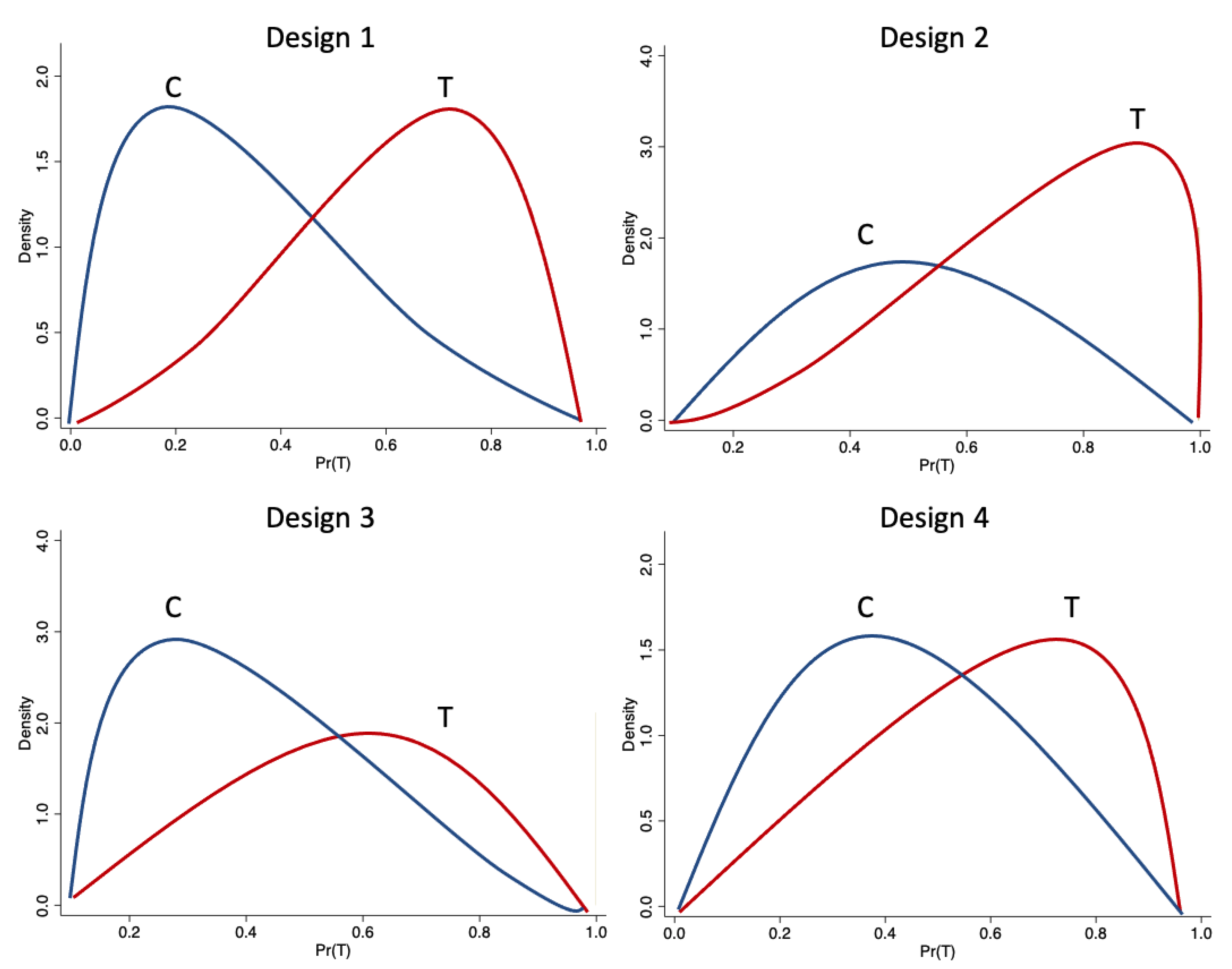
Following Frölich (2004), the propensity score is linked, through $T^{*}$, to the linear function $f\left(X_i\right)=\alpha +\beta X_i$, and through the choice of different values for $\alpha$ different ratios of control to treated observations are generated.9 The parameter $\alpha$ manages the average value of the propensity score and the number of treated relative to the number of controls in the sample. Four designs are considered; in the first (for $p=2$), $f\left(X_i\right)=0.5X_1+0.5X_2$, the population mean of the propensity score is $0.5$.10 That is, the expected ratio of control to treated observations is 1:1. In the second, $f\left(X_i\right)=0.7+0.5X_1+0.5X_2$, the ratio is 3:7 (the pool of treated observations is large), and in the third, $f\left(X_i\right)=-0.7+0.5X_1+0.5X_2$, the ratio is 7:3 (the controls greatly exceed the treated). We include these first three designs because during the estimation of the counterfactual mean, more precisely during the matching step, the effects of outliers in the treated or control groups could be offset by the number of observations in this group. The fourth design considers treatment and control groups of equal size, but with a nonlinear specification of the propensity score on the covariate of interest, $f\left(X_i\right)=0.5X_1+0.15X_1^2+0.5X_2$. In addition, $Y_i=0.15+T_i+0.5X_1+0.5X_2$, that is, the true treatment effect is 1. In the DGP we do not consider different functional forms for the conditional expectation function of $Y_i$, given $T_i$. Results from Frölich (2004) suggest that when the matching estimator uses the average, the effects of these nonlinearities may disappear.

The probability of assignment is bounded away from 0 and 1, $\varsigma <P\left(X_i\right)\equiv P(T_i=1|X_i)<1-\varsigma$, for some $\varsigma >0$, also known as strict overlap assumption, is always satisfied in these designs. Following Khan and Tamer (2010), this is a sufficient assumption for $\sqrt{n}$-consistency of semi-parametric treatment effect estimators. Busso et al. (2009) shows this when $X_i$ and ${\mu }_i$ are standard normal distributed for the linear specification of $f\left(X_i\right)$. This assumption is achieved when $\left|\beta \right|\le 1$. The intuition behind this result is that when $\beta$ approaches 1, an increasing mass of observations have propensity scores near either 0 and 1. This leads to fewer and fewer comparable observations and an effective sample size smaller than n. Significantly, this implies potentially poor finite sample properties of semi-parametric estimators in contexts where $\beta$ is near 1. In our designs, we set $\beta =0.5$ for the linear and nonlinear functions of $f\left(X_i\right)$. The overlap plots support the achievement of the strict overlap assumption for these cases, because they do not display mass near the corners. This can be observed in Figure 2, where the conditional density of the propensity score given treatment status (overlap plot) for the four designs considered in the Monte Carlo simulations are displayed.11

The second part of the design concerns the type of contamination in the sample. To grasp the influence of the outliers, we consider three contamination setups inspired by Croux and Haesbroeck (2003). The first is clean with no contamination. In the second, mild contamination, 5% of $X_1$ are awarded a value $1.5\sqrt{p}$ units larger than what the DGP would suggest. In the third, severe contamination, 5% of $X_1$ are awarded a value $5\sqrt{p}$ units larger than the DGP would suggest. As mentioned above, three types of outliers are recognized in the literature: bad leverage points, good leverage points, and vertical outliers. Nine additional scenarios can thus be considered in the analysis, depending on the localization of these outliers in the sample. That is, the three types can be located in the treatment sample (T), in the control sample (C), and in both groups (T and C). Therefore, we assess the relative performance of the estimators described in the last section in a total of 72 different contexts. These different contexts are characterized by combinations of four designs for $f\left(X_i\right)$, two types of contamination (mild and severe), and three types of outliers located in treatment, control, and in both groups, respectively.

5. The Effect of Outliers in the Estimation of Treatment Effects

5.1. The Effect of Outliers in the Metrics

Based on the artificial data set, this section presents the results by means of two simple cases, the effect of outliers in the estimation of the metrics used to define similarity and the effect of these (spurious) metrics in the assignment of matches when finding counterfactuals.

• (a) The distribution of the propensity score in presence of outliers

Using the artificial data set, we graphically show some stylized facts of the distribution of the propensity score with and without outliers. The original distribution of the propensity score by treatment status (overlap plot) corresponds to the thin lines in the left graph of Figure 3, while the thick solid lines in the left graph represent the overlap plots for the same sample, but with 5% of the data contaminated by bad leverage points in the treatment sample. As can be seen, the propensity scores are now clearly less spread out than those obtained with the original data in both the treatment and control groups. In the right graph of Figure 3, the straight line corresponds to the values of the original propensity score, whereas the cloud of points corresponds to the values of the propensity score in the presence of bad leverage points in the treatment sample; large differences in the values of the propensity score between the original and the contaminated sample are clear. Note that these effects are identical if we consider bad leverage points either in the control sample or in both the treatment and control groups.

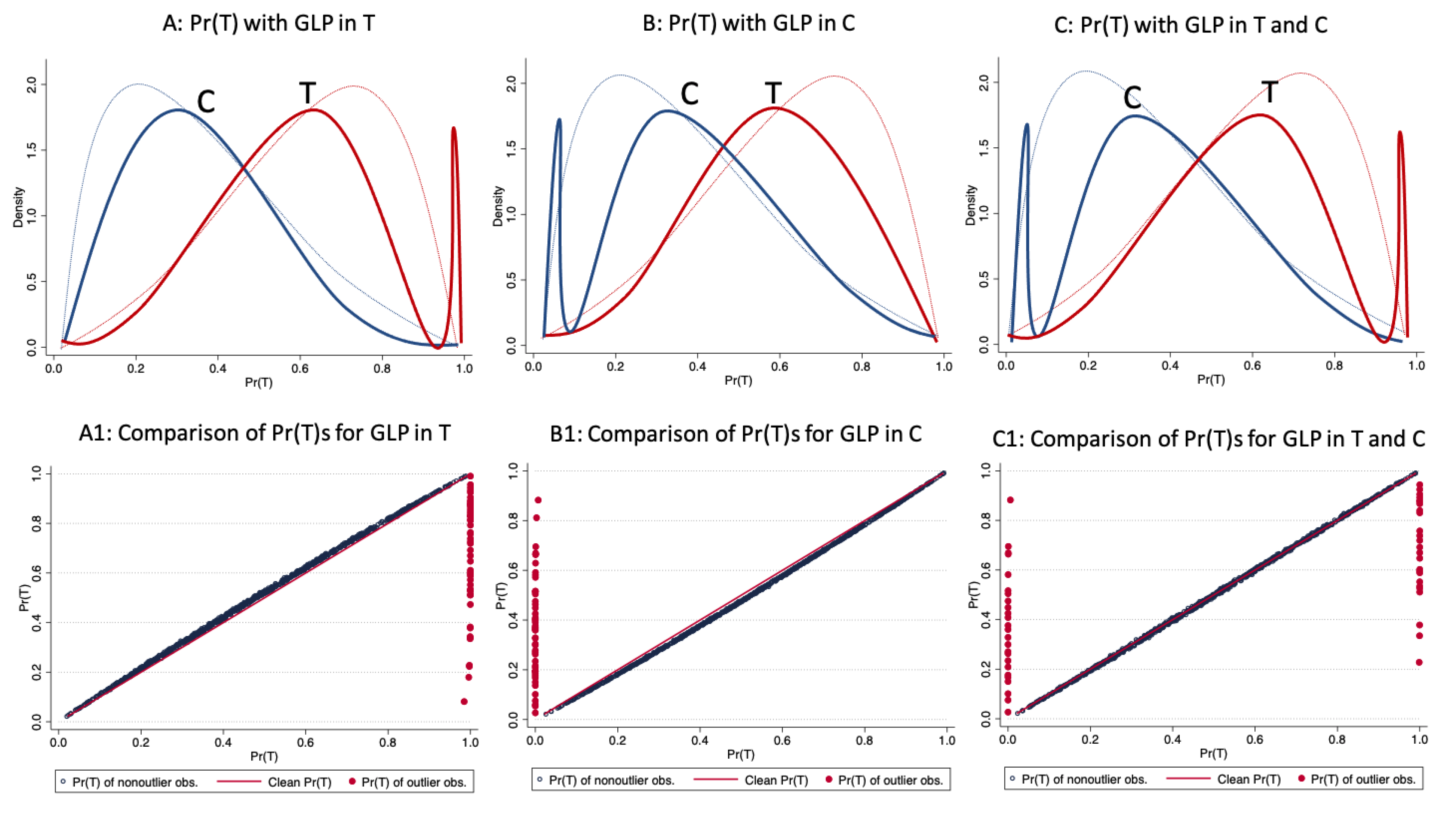
The distribution of the propensity score by treatment status in the presence of good leverage points in the treatment sample, in the control, and in both samples can be see in the top three graphs of Figure 4. In the bottom graphs, the straight line corresponds to the values of the original propensity score, whereas the cloud of points corresponds to the values of the propensity score in the presence of good leverage points. As can be observed, in contrast to bad leverage points, the good leverage points do not completely change the distribution of the propensity score.

A theoretical explanation for these results can be found in Croux et al. (2002), who showed that the non-robustness against outliers of the maximum likelihood estimator in binary models is demonstrated because it does not explode to infinity as in ordinary linear regressions, but rather implodes to zero when bad leverage outliers are present in the data set. That is, given the maximum likelihood estimator of a binary dependent variable,

$${\widehat{\beta }}_{ML}=\underset{\beta }{arg\; max}LogL(\beta ;X_n)$$

where $LogL(\beta ;X_n)$ is the log-likelihood function calculated in $\beta$. Croux et al. (2002) presented two important facts: (i) good leverage points (GLP) do not perturb the fit obtained by the ML procedure, that is ${\beta }_{ML}^{GLP}\to {\beta }_{ML}$. However, as displayed in Figure 4, the fitted probabilities of these outlying observations will be close to 0 or 1. Here, it can lead to unstable estimates of the treatment effects, because the support (or overlap) condition is not met; and (ii) in the presence of bad leverage points (BLP), the ML estimator never explodes, instead asymptotically tending to 0. That is, ${\beta }_{ML}^{BLP}\to 0$. In addition, following Frölich (2004) and Khan and Tamer (2010), coefficients close to zero in the estimation of the propensity score will then reduce the variability of the propensity score, as these coefficients $\left(\beta \right)$ determine the spread of the propensity score. Therefore, the presence of bad leverage points in the data will always narrow the distribution of the propensity score, as shown in Figure 3. As is shown below, this tightness in the distribution of the propensity score may increase the chance of matching observations with very different characteristics.

To validate these stylized facts, we applied 2000 simulations for the different scenarios of our Monte Carlo setup.

Table 1. Effect of outliers on propensity score.

Panel A: Severe contamination, ten covariates (p = 10)
		Bad Leverage Point			Good Leverage Point
Estimator	Clean	in T	in C	in T and C	in T	in C	in T and C
Coefficient (beta)	0.51	−0.05	−0.04	−0.04	0.51	0.51	0.51
MSE (×1000)	3.57	297.54	296.84	295.30	3.74	3.72	3.72
Propensity Score
Mean	0.50	0.50	0.50	0.50	0.50	0.50	0.50
Growth in Variance		−11.0%	−11.0%	−11.1%	5.0%	5.0%	4.8%
Growth in Kurtosis		5.7%	5.7%	5.8%	−1.9%	−1.8%	−1.8%
Loss in Correlation		−7.9%	−7.8%	−7.8%	−2.4%	−2.4%	−2.3%
Panel B: Severe contamination, two covariates (p = 2)
		Bad Leverage Point			Good Leverage Point
Estimator	Clean	in T	in C	in T and C	in T	in C	in T and C
Coefficient (beta)	0.50	0.00	0.00	0.00	0.51	0.51	0.51
MSE (×1000)	2.28	246.01	245.58	245.82	2.29	2.33	2.36
Propensity Score
Mean	0.50	0.50	0.50	0.50	0.50	0.50	0.50
Growth in Variance		−50.9%	−50.9%	−50.9%	19.3%	19.3%	18.4%
Growth in Kurtosis		18.0%	18.0%	18.0%	4.4%	4.3%	4.9%
Loss in Correlation		−29.7%	−29.6%	−29.6%	−8.3%	−8.3%	−8.0%
Panel C: Mild contamination, ten covariates (p = 10)
		Bad Leverage Point			Good Leverage Point
Estimator	Clean	in T	in C	in T and C	in T	in C	in T and C
Coefficient (beta)	0.51	0.09	0.09	0.09	0.53	0.53	0.52
MSE (×1000)	3.57	170.62	169.52	172.47	3.68	3.67	3.63
Propensity Score
Mean	0.50	0.50	0.50	0.50	0.50	0.50	0.50
Growth in Variance		−11.3%	−11.3%	−11.3%	5.0%	5.0%	4.8%
Growth in Kurtosis		6.1%	6.1%	6.1%	−2.1%	−2.1%	−2.0%
Loss in Correlation		−29.7%	−29.6%	−29.6%	−8.3%	−8.3%	−8.0%
Panel D: Mild contamination, two covariates (p = 2)
		Bad Leverage Point			Good Leverage Point
Estimator	Clean	in T	in C	in T and C	in T	in C	in T and C
Coefficient (beta)	0.50	0.29	0.29	0.28	0.55	0.55	0.55
MSE (×1000)	2.28	46.35	46.33	47.86	4.32	4.40	4.19
Propensity Score
Mean	0.50	0.50	0.50	0.50	0.50	0.50	0.50
Growth in Variance		−29.3%	−29.3%	−29.6%	17.1%	17.1%	16.7%
Growth in Kurtosis		9.3%	9.4%	9.4%	−3.0%	−3.0%	−2.6%
Loss in Correlation		−6.3%	−6.2%	−6.5%	−3.8%	−3.8%	−3.9%

Note: The results correspond to the propensity score metric and 2000 replications. The estimator section depicts the mean and MSE of the probit coefficients. The propensity score section shows characteristics of the propensity score. Each column represents a contamination type and placement: Clean; BLP; GLP, in treatment group (T), in control group (C) and both. Panels A through D represent different combinations of contamination levels and number of covariates.

provides the results in four panels, each corresponding to a scheme with different outlier contamination levels (mild and severe) and different number of covariates $(p=2 \mathrm{and} p=10)$. The sample size is 1000 observations and the specification of the propensity score corresponds to the first design, that is, as a linear function with equal number of observations in both treatment and control groups.12 This implies that we first obtain the propensity score. Once the propensity score is calculated, it is possible to characterize it through its mean, variance, kurtosis, skewness. It is also possible to calculate the correlation between the propensity score in the clean scenario and the propensity score of any of the contaminated scenarios.13 Thus, the growth in variance is the percentage change of the variance of the propensity score in a specific scenario vs. the variance in the clean scenario; for example, for the BLP in the treatment group, this would mean that the variance of the propensity score of the contaminated data is $11.0\%$ lower than in the clean data. The same reasoning applies to the growth in kurtosis. This reinforces what was observed in the left panel of Figure 3 where we can see that the variance of the contaminated data is lower and it is more leptokurtic.

The loss in correlation corresponds to the change in correlation between the propensity score of a given scenario vs. clean data. That is, for the BLP in the treatment scenario, the correlation of the propensity score between the contaminated data and clean data is 7.9% lower with respect to the clean data. That is, the correlation of the clean propensity score with itself is 100%, while the correlation between the contaminated propensity score and the clean propensity score is 92.1%, representing a loss in correlation of 7.9%.

The results are summarized in two sections of Table 1. The first presents estimates of the average absolute value of the coefficient of interest $\left(\beta \right)$ and its mean squared error (MSE) multiplied by a factor of 1000, and the second presents the characteristics of the propensity score: its average value, variance growth, kurtosis, and loss of the correlation, all four of them compared to their baseline scenario values. The columns represent different degrees of outlier contamination.

Regarding the parameter $\beta$ in the specification of the propensity score, the true value is 0.5; the Clean column confirms that the simulation results for the baseline scenario are extremely close to the true parameter. The remaining columns show that in presence of bad leverage points, the coefficient diverges from the true value, tending towards 0. By contrast, if the variable contains good leverage points, the regression coefficient remains unbiased. The behavior in each case is independent of the location of the leverage points. When focusing on the characteristics of the propensity score, several features stand out. First, outliers do not change the center of the propensity score distribution, since the mean is identical across different contamination scenarios. Second, the form of the distribution is affected, because bad leverage points shrink the density of the propensity score. This is evidenced by the reduction in the variance and the rise in the kurtosis when this type of outlier is present in the data. As can be seen in Table 1, this effect is larger when the outlyingness level is greater and when lesser covariates are present in the estimation of the propensity score. Theoretically, this result is in line with Frölich (2004) and Khan and Tamer (2010), who suggest that coefficients close to 0 in the estimation of the propensity score, ${\beta }_{ML}^{BLP}\to 0$, reduce the variability of this metric, as these coefficients $\left(\beta \right)$ determine the spread of the propensity score.

Third, good leverage points have the opposite effect on the shape of the propensity score—that is, the dispersion increases and the kurtosis is reduced. These variations are however lower compared to those of bad leverage points. This happens because good leverage points nearly attain the extreme values of the propensity score (0 or 1), without significantly changing the complete distribution of this metric. Fourth, the propensity score contaminated by both type of outliers is less related to the score corresponding to the baseline scenario. This is revealed by the reduction of the linear correlation between the baseline propensity score and the score with outliers. This reduction in the linear association is strong with bad leverage points and weak with good leverage points in the data. All these effects remain independent of the outlier location.

The effect of these distortions in the density of the propensity score in the matching process and in the treatment effect estimation is discussed in following sections.

• (b) The distribution of the Mahalanobis distance in presence of outliers

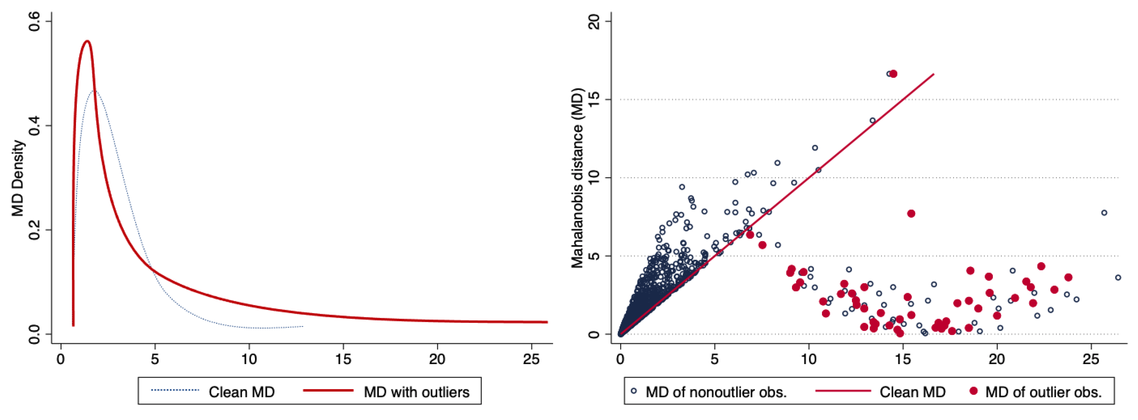
As in the case of the propensity score matching, the left side of Figure 5 shows the the distributions of the Mahalanobis distance without outliers and in the presence of bad leverage points. In the right graph, the straight line corresponds to the values of the Mahalanobis distance computed with the clean data, whereas the cloud of points corresponds to the values of this metric in the presence of bad leverage points in the treatment group; the blue observations correspond to non-outlier observations while the red ones are the outliers.

Three remarks can be made on the basis of these graphs. First, good and bad leverage points present atypical behavior in the sense that they display larger distances. Since Mahalanobis distances are computed individually for each observation, bad and good leverage points present bigger values, whereas the remaining observations stay relatively stable. This behavior is independent of the location of the outlier. Second, while bad and good leverage points slightly change the distribution of the distances, the stability of the not contaminated observations is relative, in the sense that all distances are standardized by the sample covariance matrix of the covariates $\left(S^{-1}\right)$, which is in turn based on biased measures (due to the outliers) of the averages and variances in the sample. Third, concluding that observations with large distances can directly be called outliers may be fallacious, just in the sense that to be called outliers these distances need to be estimated by a procedure that is robust against outliers in order to provide reliable measures for the recognition of outliers. This is the masking effect Rousseeuw and Van Zomeren (1990). Single extreme observations or groups of observations, departing from the main data structure, can have a heightened influence on this distance measure, because the covariance $\left(S^{-1}\right)$ is estimated in a non-robust manner, that is, it is biased.

Table 2. Effect of outliers on the Mahalanobis distance.

Panel A: Severe contamination, ten covariates (p = 10)
		Bad Leverage Point			Good Leverage Point
Mahalanobis Distance	Clean	in T	in C	in T and C	in T	in C	in T and C
Mean	2.00	2.04	2.04	2.00	2.04	2.04	2.00
Growth in Variance		395.0%	394.5%	361.0%	398.8%	398.6%	364.2%
Growth in Asymmetry		89.6%	89.5%	87.7%	89.6%	89.6%	87.7%
Growth in Kurtosis		95.9%	95.6%	93.1%	95.7%	95.4%	92.7%
Loss in Correlation		−76.3%	−76.3%	−75.6%	−75.4%	−75.4%	−74.7%
Panel B: Severe contamination, two covariates (p = 2)
		Bad Leverage Point			Good Leverage Point
Mahalanobis Distance	Clean	in T	in C	in T and C	in T	in C	in T and C
Mean	2.00	2.02	2.02	2.00	2.03	2.03	2.00
Growth in Variance		206.6%	207.5%	199.2%	234.6%	234.9%	222.7%
Growth in Asymmetry		86.7%	87.0%	85.6%	88.3%	88.4%	87.0%
Growth in Kurtosis		112.4%	112.9%	110.1%	111.1%	111.4%	108.9%
Loss in Correlation		−64.3%	−64.0%	−64.0%	−63.8%	−63.5%	−63.3%
Panel C: Mild contamination, ten covariates (p = 10)
		Bad Leverage Point			Good Leverage Point
Mahalanobis Distance	Clean	in T	in C	in T and C	in T	in C	in T and C
Mean	2.00	2.01	2.01	2.00	2.02	2.02	2.00
Growth in Variance		106.6%	106.2%	106.3%	129.7%	129.6%	127.1%
Growth in Asymmetry		76.5%	75.8%	76.3%	81.5%	81.0%	80.3%
Growth in Kurtosis		118.8%	116.5%	117.1%	121.8%	120.5%	118.3%
Loss in Correlation		−49.2%	−49.1%	−49.6%	−50.4%	−50.3%	−50.7%
Panel D: Mild contamination, two covariates (p = 2)
		Bad Leverage Point			Good Leverage Point
Mahalanobis Distance	Clean	in T	in C	in T and C	in T	in C	in T and C
Mean	2.00	2.00	2.00	2.00	2.00	2.00	2.00
Growth in Variance		1.7%	2.0%	2.3%	19.2%	19.2%	19.8%
Growth in Asymmetry		3.4%	3.5%	4.4%	21.6%	21.3%	22.2%
Growth in Kurtosis		7.0%	6.9%	9.0%	37.6%	36.9%	38.1%
Loss in Correlation		−7.8%	−7.8%	−8.3%	−17.7%	−17.6%	−18.2%

Note: The results correspond to the Mahalanobis distance metric and 2000 replications. The statistics presented are comparable to the ones in Table 1. Each column represents a contamination type and placement: Clean; BLP; GLP, in treatment group (T), in control group (C) and both. Panels A through D represent different combinations of contamination levels and number of covariates.

reports the simulations for the behavior of the Mahalanobis distance under the different contaminated-data scenarios. The outlier intensity is displayed in panels A to D and the outlier location is displayed in the columns. In each panel, the average of the distances, the growth of the Mahalanobis distance variance, asymmetry, kurtosis, and linear correlation with respect to the clean data scheme are displayed. The results correspond to 2000 simulations for the first design of our Monte Carlo setup.14 We turn first to the results in the center of the distribution: as can be seen, no leverage point changes the mean of the Mahalanobis distances, whereas outliers distort the shape of this metric distribution.

Managed by the extreme values of the distances corresponding to the outlier observations, the variance increases abruptly and the distribution skews positively and turns more leptokurtic, as shown in Figure 5. These characteristics are independent of the location of outliers. In addition, as displayed in the last row of each panel in Table 2, the distances in presence of outliers are significantly less linearly related to the original Mahalanobis distances.

Overall, the results of this section suggest the distribution of the Mahalanobis distance becomes narrower and with long tails in the presence of bad and good leverage points in the data. This effect is a combination of two factors: outlier observations are associated with the largest values of the distances and all distances change as they are standardized with a covariance matrix distorted by outliers. This behavior of the Mahalanobis distance suggests a way to detect the presence of outliers in the sample.

5.2. The Matching Process in the Presence of Outliers, a Toy Example

To illustrate the effect of outliers on the assignment of matches when finding counterfactuals we use a small data set consisting on fifteen normally distributed observations for the first design of our DGP are generated. These variables are presented in columns 1–4 of

Table 3. Effect of a bad and a good leverage point on matching assignment.

Col:	(1)	(2)	(3)	(4)	(5)	(6)	(7)	(8)	(9)	(10)	(11)	(12)	(13)	(14)	(15)	(16)
								Propensity Score						Covariate Matches
	Original Data				Propensity Score			Matches (ID)			Mahalanobis Distance			(ID)
ID	y	x1	x2	T	P(T)o	P(T)blp	P(T)glp	mo	mblp	mglp	MDo	MDblp	MDglp	mo	mblp	mglp
1	0.94	0.35	−1.14	T	0.27	0.30	0.28	14	11	14	0.62	0.62	0.61	12	11	11
2	2.58	0.58	−0.06	T	0.78	0.47	0.75	12	15	12	0.51	0.02	0.26	12	12	12
3	2.29	1.41	0.67	T	0.99	0.55	0.99	12	9	12	4.40	0.90	1.78	15	13	8
4	1.45	−0.79	0.68	T	0.52	0.65	0.56	8	8	8	0.66	1.19	0.55	12	14	11
5	1.27	−0.83	0.04	T	0.25	0.55	0.30	14	9	14	0.63	0.78	0.04	12	11	9
6	1.08	0.87	0.36	T	0.93	0.52	0.92	12	9	12	1.73	0.28	0.82	13	9	11
7	2.21	0.35	1.15	T	0.96	0.68	0.95	12	8	12	2.37	1.21	1.98	8	14	8
8	−0.72	−1.58	1.50	C	0.51	0.79	0.59				2.60	3.74	1.94
9	1.26	−0.17	−0.08	C	0.47	0.50	0.49				0.02	0.18	0.04
10	−1.47	1.74	−3.12	C	0.13	0.06	0.10				5.98	6.52	5.88
11	0.52	−0.25	−1.00	C	0.13	0.35	0.16				0.91	0.69	0.50
12	0.04	0.75	−0.51	C	0.68	0.38	0.66				0.50	0.11	0.23
13	−0.10	−0.61	−0.90	C	0.08	0.38	0.11				1.39	0.88	0.46
14	−0.08	0.30	−1.48	C	0.16	0.26	0.16				1.24	1.14	1.16
15	−1.53	−2.30	1.16	C	0.14	0.49	0.00				4.42	9.75	11.74

. The exercises consist on artificially substituting the value of one observation in one covariate and observing in detail its effect on the matches assigned. One bad and one good leverage point is generated by moving the value of the first treated observation of $X_1$ by $-5\sqrt{2}$ and by $+5\sqrt{2}$, respectively (severe contamination). Columns 5 to 7, and 11 to 13 of Table 3 present the propensity score and the Mahalanobis distance estimated with the original and contaminated data. As can be seen, the distribution of the propensity score and the Mahalanobis distance with bad leverage points completely changes. Observations 2 and 3, for example, change their probability of participating in the program from 0.78 to 0.47 and from 0.99 to 0.55 when looking at the propensity score matching and from 0.51 to 0.02 and from 4.40 to 0.90 when examining the Mahalanobis distance.

The distribution of the propensity score with good leverage points keeps to the same path. Columns 8 to 10 show the consequent effect of the variation in this metric on the matches assigned to generate the counterfactuals (by using the nearest neighbor criteria).15 Consider observations 5 and 6, for example. Initially, observations 14 and 12 are presented as counterfactual observations, but due to the presence of the bad leverage point, the nearest observation now corresponds to observation 9 in both cases. The matches assigned in the presence of good leverage points are the same as the original data. Columns 11 to 13 show the behavior of the Mahalanobis distance. Unlike the propensity score matching, the toy example shows that there are also significant changes when examining good leverage points in the Mahalanobis distance. Thus, the presence of outliers may distort even more the treatment effects when using this estimand.

For a proper estimation of the unobserved potential outcomes, we want to compare treated and control groups that are as similar as possible. These simple illustrations explain that extreme values can easily distort the metrics used to define similarity and thus may bias the estimates of treatment effects by making the groups very different. That is, the prediction of ${\widehat{Y}}_i^0$ for the treated group is made using information from observations that are different from themselves. In the next section, we present evidence about the effects on the treatment effect estimation.

5.3. The Effect of Outliers on the Different Matching Estimators

In this section we examine the effect of outliers on the estimation of treatment effects under different scenarios and through a set of matching estimators.

Table 4. Simulated bias and MSE of Average Treatment Effect on the Treated (TOT) estimates in the presence of outliers using propensity score.

Panel A: Severe contamination, ten covariates (p = 10)
		Bad Leverage Point			Good Leverage Point			Vertical Outliers in Y
Estimator	Clean	in T	in C	in T and C	in T	in C	in T and C	in T	in C	in T and C
BIAS (×1000)
Pair Matching	155.72	536.54	568.73	547.42	43.91	162.42	100.70	1738.27	−1425.95	160.84
Ridge M. Epan	143.49	501.50	525.45	511.43	48.85	151.99	105.46	1725.28	−1428.19	153.34
IPW	299.37	634.05	636.05	632.63	299.32	300.98	297.69	1881.92	−1264.44	309.81
Pair Matching (bias corrected)	−1.48	785.56	433.26	461.78	−797.19	−4.43	−398.52	1581.07	−1570.68	9.77
MSE (×1000)
Pair Matching	112.73	353.53	384.21	361.60	134.13	121.73	122.59	3113.71	3808.92	1005.98
Ridge M. Epan	93.06	301.00	320.69	308.11	106.14	100.44	100.95	3053.33	3406.23	760.11
IPW	164.17	459.52	464.34	458.64	164.85	172.71	167.73	3619.12	2173.43	421.42
Pair Matching (bias corrected)	61.73	669.61	234.13	258.86	857.37	65.18	283.12	2564.56	3774.03	735.33
		Bad Leverage Point			Good Leverage Point			Vertical Outliers in Y
Estimator	Clean	in T	in C	in T and C	in T	in C	in T and C	in T	in C	in T and C
BIAS (×1000)
Pair Matching	9.13	367.76	367.39	364.36	−112.22	10.93	−50.59	717.27	−705.47	12.48
Ridge M. Epan	0.29	362.47	362.71	361.51	−74.07	1.11	1.80	709.29	−710.40	2.20
IPW	16.56	366.56	366.76	366.70	13.15	14.52	14.14	724.71	−694.33	18.71
Pair Matching (bias corrected)	−0.05	354.12	363.51	359.18	−353.72	1.14	−176.80	708.10	−714.09	3.67
MSE (×1000)
Pair Matching	13.17	145.73	145.98	143.36	42.97	14.28	22.53	528.13	557.91	36.83
Ridge M. Epan	8.70	138.96	139.35	138.48	26.19	9.39	9.22	512.84	535.14	19.80
IPW	11.37	140.60	140.75	140.72	11.44	12.32	11.91	536.91	512.48	20.91
Pair Matching (bias corrected)	13.17	134.87	143.09	139.57	184.52	14.30	59.37	515.14	571.01	37.00
Panel C: Mild contamination, ten covariates (p = 10)
		Bad Leverage Point			Good Leverage Point			Vertical Outliers in Y
Estimator	Clean	in T	in C	in T and C	in T	in C	in T and C	in T	in C	in T and C
BIAS (×1000)
Pair Matching	155.72	446.02	478.72	465.70	49.10	163.02	104.01	630.48	−318.78	157.26
Ridge M. Epan	143.49	407.01	434.69	422.19	52.56	150.44	104.68	618.03	−328.02	146.44
IPW	299.37	553.26	555.45	557.44	288.31	289.99	287.53	774.14	−169.77	302.51
Pair Matching (bias corrected)	−1.48	236.68	376.49	350.68	−240.05	−2.05	−118.73	473.28	−472.24	1.89
MSE (×1000)
Pair Matching	112.73	262.10	289.80	278.70	130.69	120.45	119.56	486.58	342.40	193.33
Ridge M. Epan	93.06	212.60	234.28	223.57	104.30	100.14	99.52	455.07	297.76	153.73
IPW	164.17	361.29	367.50	367.74	160.30	168.08	163.66	674.21	147.06	188.24
Pair Matching (bias corrected)	61.73	100.48	187.36	170.06	151.11	66.23	90.72	286.13	398.70	121.23
Panel D: Mild contamination, two covariates (p = 2)
		Bad Leverage Point			Good Leverage Point			Vertical Outliers in Y
Estimator	Clean	in T	in C	in T and C	in T	in C	in T and C	in T	in C	in T and C
BIAS (×1000)
Pair Matching	9.13	127.38	204.31	175.95	−79.71	−3.21	−40.49	221.57	−205.25	10.13
Ridge M. Epan	0.29	125.16	183.86	160.66	−67.73	−14.64	−38.13	212.99	−212.92	0.86
IPW	16.56	166.69	166.07	168.93	−16.22	−14.88	−13.95	229.01	−196.71	17.21
Pair Matching (bias corrected)	−0.05	105.04	199.85	172.82	−106.54	−13.39	−58.22	212.40	−214.26	1.07
MSE (×1000)
Pair Matching	13.17	27.84	52.39	43.02	25.87	13.98	17.67	62.24	59.63	15.40
Ridge M. Epan	8.70	23.30	41.90	33.80	15.14	9.56	11.09	54.14	56.18	9.77
IPW	11.37	35.14	36.07	36.43	12.83	13.38	13.05	63.62	51.76	12.18
Pair Matching (bias corrected)	13.17	22.53	50.49	41.89	31.93	14.24	19.74	58.35	63.53	15.40

Note: The results use the propensity score metric and 2000 replications. The statistics presented are the bias and MSE of each estimator (Pair matching, Ridge, IPW and bias corrected Pair matching) scaled by 1000. The bias is calculated by subtracting the true effect of the treatment (1) from the estimate of TOT. Each column represents a contamination type and placement: Clean; BLP; GLP; and vertical outliers, in treatment group (T), in control group (C) and both. Panels A through D represent different combinations of contamination levels and number of covariates.

shows the performance in the estimation of the average treatment effect on the treated of the four selected estimators for the first design of our DGP. It presents the bias and the mean squared error, from 2000 replications. The sample size $\left(n\right)$ is 1000 and the number of covariates is $p\in \{2,10\}$. The four panels resemble the panels presented in Table 1. However, in this case, columns correspond to the type of outlier and rows to the estimators. Column 1, called clean, involves the no-contamination scenario. Columns 2–4 contain bad leverage points in the treatment, control, and both groups simultaneously, respectively. Similarly, columns 5–7 consider good leverage points, whereas columns 8–10 correspond to vertical outliers in the treatment, control, and in both samples, respectively. To compute the bias, we first, calculated the bias of the estimate, for example pair matching, by subtracting the true effect off the treatment estimator; that is: $bias=({\beta }_{TOT}^{pairmatching}-1)$, the same was done for each of the scenarios and the result (scaled by 1000) can be found in Table 4.16

The results suggest several important conclusions. First, in the absence of outliers all the estimators we considered perform well, which is in accordance with the evidence provided by Busso et al. (2009) and Busso et al. (2014); however, there is a larger bias in the estimate when more covariates are present, regardless of the level of contamination. The bias-corrected covariate matching of Abadie and Imbens (2011) has the smallest bias, followed by the local linear ridge propensity score matching, the pair matching estimator, and the reweighting estimator based on the propensity score. Second, in the presence of bad leverage points, all the estimates present a considerable bias. For the propensity score matching methods, the size of the bias is generally the same, independent of the location of the outlier. This is expected because, as explained in the last section, the complete distribution of the metrics changes when bad leverage points exist in the data. The spread of the metrics decreases and observations that initially presented larger (lower) values of the metric may now match with observations that initially had lower (larger) values. Therefore, for pair matching the spurious metric will match inappropriate controls. For local linear ridge matching, the weights $W_{i,j}$, which are a function (kernel) of the differences in the propensity score, will decrease notably. In the case of the reweighted estimator, some control observations will receive higher weights, because their propensity score values are higher than those values from the original data, and some will receive lower weights (as the weights are normalized to sum up to 1). Finally, for the bias corrected pair matching, there is a clear difference for the clean data, since the correction reduces the bias of the clean data, however, the bias correction does not reduce the bias in contaminated groups.

For the multivariate distance matching estimators using Mahalanobis distance, results are very similar and can be found in

Table A1. Simulated bias and MSE of Average Treatment Effect on the Treated (TOT) estimates in the presence of outliers using Mahalanobis distance.

Panel A: Severe contamination, ten covariates (p = 10)
		Bad Leverage Point			Good Leverage Point			Vertical Outliers in Y
Estimator	Clean	in T	in C	in T and C	in T	in C	in T and C	in T	in C	in T and C
BIAS (×1000)
Pair Matching	1086.22	1223.63	1119.44	1172.59	1157.35	1178.44	1168.45	2668.76	−489.12	1088.07
Ridge M. Epan	842.51	720.66	919.31	843.54	693.92	996.84	895.42	2425.10	−740.40	839.84
IPW	299.37	634.05	636.05	632.63	299.32	300.98	297.69	1881.92	−1264.44	309.81
Pair Matching (bias corrected)	−0.30	784.72	−4.07	390.26	−794.54	−2.97	−398.78	1582.25	−1561.61	5.80
MSE (×1000)
Pair Matching	1195.58	1512.29	1269.62	1390.48	1354.94	1405.09	1380.86	7140.02	389.79	1270.85
Ridge M. Epan	728.11	545.59	864.04	731.77	510.25	1012.31	821.86	5901.36	736.89	810.76
IPW	164.17	459.52	464.34	458.64	164.85	172.71	167.73	3619.12	2173.43	421.42
Pair Matching (bias corrected)	33.63	647.77	34.49	179.25	705.14	34.03	206.16	2539.83	3115.53	385.02
Panel B: Severe contamination, two covariates (p = 2)
		Bad Leverage Point			Good Leverage Point			Vertical Outliers in Y
Estimator	Clean	in T	in C	in T and C	in T	in C	in T and C	in T	in C	in T and C
BIAS (×1000)
Pair Matching	30.91	208.75	36.59	122.37	−44.75	38.48	−2.37	739.06	−677.65	32.78
Ridge M. Epan	10.32	18.98	13.36	11.95	−29.65	15.18	13.39	718.08	−698.28	11.13
IPW	16.56	366.56	366.76	366.70	13.15	14.52	14.14	724.71	−694.33	18.71
Pair Matching (bias corrected)	−0.45	352.34	3.28	176.75	−351.72	0.43	−175.19	707.70	−709.09	1.41
MSE (×1000)
Pair Matching	11.98	58.24	12.97	26.70	18.82	12.97	12.71	557.67	501.67	28.60
Ridge M. Epan	8.29	9.41	8.89	8.62	9.03	8.87	8.62	524.74	513.96	17.84
IPW	11.37	140.60	140.75	140.72	11.44	12.32	11.91	536.91	512.48	20.91
Pair Matching (bias corrected)	11.53	144.05	12.26	43.13	162.99	12.16	49.71	512.82	549.09	29.90
		Bad Leverage Point			Good Leverage Point			Vertical Outliers in Y
Estimator	Clean	in T	in C	in T and C	in T	in C	in T and C	in T	in C	in T and C
BIAS (×1000)
Pair Matching	1086.22	1159.95	1082.64	1121.85	1095.43	1130.02	1112.92	1560.98	613.62	1086.77
Ridge M. Epan	842.51	834.56	841.42	837.11	756.97	924.32	844.29	1317.29	367.63	841.70
IPW	299.37	553.26	555.45	557.44	288.31	289.99	287.53	774.14	−169.77	302.51
Pair Matching (bias corrected)	−0.30	233.96	115.19	163.37	−242.97	4.65	−118.03	474.47	−468.69	1.53
MSE (×1000)
Pair Matching	1195.58	1360.56	1188.79	1274.27	1215.94	1293.03	1254.26	2452.46	403.96	1202.47
Ridge M. Epan	728.11	715.45	727.87	720.04	593.99	873.91	732.86	1753.60	167.95	733.91
IPW	164.17	361.29	367.50	367.74	160.30	168.08	163.66	674.21	147.06	188.24
Pair Matching (bias corrected)	33.63	81.71	49.12	56.58	102.09	35.63	51.16	259.04	311.60	64.86
Panel D: Mild contamination, two covariates (p = 2)
		Bad Leverage Point			Good Leverage Point			Vertical Outliers in Y
Estimator	Clean	in T	in C	in T and C	in T	in C	in T and C	in T	in C	in T and C
BIAS (×1000)
Pair Matching	30.91	130.59	170.19	164.75	−38.46	20.82	−8.39	243.35	−181.66	31.47
Ridge M. Epan	10.32	107.76	151.50	141.35	−50.88	−1.65	−21.12	222.65	−202.26	10.57
IPW	16.56	166.69	166.07	168.93	−16.22	−14.88	−13.95	229.01	−196.71	17.21
Pair Matching (bias corrected)	−0.45	105.94	156.04	148.67	−104.89	−12.24	−58.01	212.00	−213.04	0.11
MSE (×1000)
Pair Matching	11.98	27.17	39.59	37.51	15.41	12.14	12.50	70.27	46.86	13.48
Ridge M. Epan	8.29	19.21	31.03	27.80	11.83	8.77	9.22	57.82	50.73	9.11
IPW	11.37	35.14	36.07	36.43	12.83	13.38	13.05	63.62	51.76	12.18
Pair Matching (bias corrected)	11.53	21.63	35.20	32.71	26.99	12.51	16.96	56.51	60.10	13.21

Note: The results use the Mahalanobis distance metric and 2000 replications. The statistics presented are the bias and MSE of each estimator (Pair matching, Ridge, IPW and bias corrected Pair matching) scaled by 1000. The bias is calculated by subtracting the true effect of the treatment (1) from the estimate of TOT. Each column represents a contamination type and placement: Clean; BLP; GLP; and vertical outliers, in treatment group (T), in control group (C) and both. Panels A through D represent different combinations of contamination levels and number of covariates.

in Appendix A. Treatment observations with bad leverage points bias the treatment effect estimates as the distribution of the distances changes completely. Moreover, outlier observations present larger values for the metric and are matched to inappropriate controls. Bad leverage points in the control sample have little effect on the estimates of average treatment effect for the treated, because the distribution of the distances changes completely, but outlier observations are less likely to be considered as counterfactuals.

Third, good leverage points in the treatment sample also bias the treatment effect estimates of the propensity score matching estimators. Good leverage points in the treatment sample have estimates of the probability of receiving treatment close to 1. These treated observations with outlying values lack suitable controls against which to compare them. This violates the overlap assumption and therefore increases the likelihood of biasing the matching estimates. In the case of the reweighted estimator, the unbiasedness is explained as just the outliers receiving higher weights, while remaining observations present almost the same weight (slightly modified by a normalization procedure). Moreover, good leverage points in the treatment group yield a great bias of the covariate matching estimator. This effect, which is similar to those coming from bad leverage points, is explained by these outlying observations having larger values for the metric and therefore being matched to inappropriate controls.

Fourth, good leverage points in the control sample do not affect matching methods. For the propensity score matching estimates, the values of the propensity score for the outliers are close to 0; these observations would cause little difficulty, because they are unlikely to be used as matches. For the reweighted estimator, these outlying observations would get close to zero weighting. For the covariate matching estimators, good leverage points in the control sample have little effect on the estimates, because such observations are less likely to be considered as counterfactuals. Fifth, when good leverage points are presented in both samples, treatment effect estimates are biased. This bias probably comes from the outliers in the treatment group. Sixth, vertical outliers bias the treatment effect estimates. This bias is easy to understand, because extreme values in the outcomes, $Y_i^1$ or $Y_i^0$, will move the average values toward them in their respective groups, independent of the estimator used to match the observations. Seventh, the immediate effect of outliers is to reject the balancing hypothesis. It is noteworthy that very similar results are obtained when estimating the Average Treatment Effect (ATE). Results can be found

Table A2. Simulated bias and MSE of Average Treatment Effect (ATE) estimates in the presence of outliers using propensity score.

Panel A: Severe contamination, ten covariates (p = 10)
		Bad Leverage Point			Good Leverage Point			Vertical Outliers in Y
Estimator	Clean	in T	in C	in T and C	in T	in C	in T and C	in T	in C	in T and C
BIAS (×1000)
Pair Matching	157.33	555.59	554.08	549.96	104.26	106.62	102.91	1766.01	−1425.13	178.94
Ridge M. Epan	147.88	515.87	513.57	513.06	104.64	104.81	109.83	1755.33	−1429.67	173.25
IPW	302.65	638.80	638.05	637.00	305.49	303.68	303.62	1900.85	−1270.70	320.41
Pair Matching (bias corrected)	−1.46	610.43	613.04	463.74	−400.41	−397.05	−397.35	1599.17	−1577.66	15.82
MSE (×1000)
Pair Matching	71.59	343.59	342.04	337.37	70.16	72.50	69.81	3603.22	2511.61	556.46
Ridge M. Epan	61.16	293.04	291.05	290.18	59.08	59.91	60.06	3463.70	2415.09	436.35
IPW	127.18	438.55	437.76	436.00	129.61	129.60	128.99	3804.20	1777.43	290.78
Pair Matching (bias corrected)	33.22	400.58	402.54	240.62	236.94	233.46	224.63	2918.21	2843.96	389.60
		Bad Leverage Point			Good Leverage Point			Vertical Outliers in Y
Estimator	Clean	in T	in C	in T and C	in T	in C	in T and C	in T	in C	in T and C
BIAS (×1000)
Pair Matching	6.77	365.94	367.44	363.69	−52.71	−53.61	−52.90	715.82	−704.41	9.01
Ridge M. Epan	−1.26	361.99	362.35	361.20	−39.69	−38.78	−1.32	707.99	−710.25	0.59
IPW	15.14	366.01	365.67	365.88	11.74	12.45	12.60	724.58	−694.08	16.83
Pair Matching (bias corrected)	−2.53	357.08	359.43	358.67	−178.27	−180.27	−179.55	706.65	−713.44	−0.06
MSE (×1000)
Pair Matching	8.93	141.38	142.58	139.63	16.61	16.57	15.16	532.34	517.66	21.31
Ridge M. Epan	6.56	137.26	137.50	136.73	11.45	11.32	6.99	513.77	517.40	12.91
IPW	7.49	139.29	139.04	139.22	7.77	7.71	7.69	537.06	494.29	12.61
Pair Matching (bias corrected)	8.98	134.52	136.12	135.97	53.05	53.97	48.70	519.86	530.76	21.61
Panel C: Mild contamination, ten covariates (p = 10)
		Bad Leverage Point			Good Leverage Point			Vertical Outliers in Y
Estimator	Clean	in T	in C	in T and C	in T	in C	in T and C	in T	in C	in T and C
BIAS (×1000)
Pair Matching	157.33	463.05	462.51	465.78	106.34	109.70	105.85	639.93	−317.41	163.81
Ridge M. Epan	147.88	421.79	420.59	423.28	105.66	106.37	109.36	630.12	−325.38	155.49
IPW	302.65	557.12	555.97	558.83	294.72	293.01	293.63	782.11	−169.35	307.98
Pair Matching (bias corrected)	−1.46	308.67	305.55	352.88	−120.19	−119.79	−118.44	478.73	−474.32	3.72
MSE (×1000)
Pair Matching	71.59	247.91	247.32	249.98	70.09	72.02	68.68	492.73	188.26	116.46
Ridge M. Epan	61.16	203.29	202.74	204.07	58.90	59.87	59.55	465.08	175.98	96.51
IPW	127.18	339.96	338.72	342.15	123.97	124.03	123.85	659.32	75.26	143.62
Pair Matching (bias corrected)	33.22	119.82	118.23	149.90	58.48	58.29	56.14	289.87	288.91	64.86
Panel D: Mild contamination, two covariates (p = 2)
		Bad Leverage Point			Good Leverage Point			Vertical Outliers in Y
Estimator	Clean	in T	in C	in T and C	in T	in C	in T and C	in T	in C	in T and C
BIAS (×1000)
Pair Matching	6.77	166.49	165.31	176.44	−43.12	−43.16	−42.81	219.49	−206.58	7.44
Ridge M. Epan	−1.26	155.43	153.36	160.93	−42.85	−42.41	−39.68	211.52	−213.96	−0.70
IPW	15.14	166.26	164.94	167.79	−17.68	−16.96	−15.55	227.97	−197.63	15.64
Pair Matching (bias corrected)	−2.53	153.08	151.58	173.31	−61.94	−62.04	−60.94	210.22	−215.81	−1.79
MSE (×1000)
Pair Matching	8.93	35.45	35.23	39.21	12.64	12.98	12.27	58.07	52.79	10.18
Ridge M. Epan	6.56	30.34	29.67	32.10	9.13	9.16	8.72	51.85	52.98	7.20
IPW	7.49	33.43	33.06	34.04	8.57	8.42	8.35	59.68	46.86	7.94
Pair Matching (bias corrected)	8.98	31.11	30.81	38.08	14.93	15.24	14.31	54.25	56.78	10.23

Note: The results use the propensity score metric and 2000 replications. The statistics presented are the bias and MSE of each estimator (Pair matching, Ridge, IPW and bias corrected Pair matching) scaled by 1000. The bias is calculated by subtracting the true effect of the treatment (1) from the estimate of TOT. Each column represents a contamination type and placement: Clean; BLP; GLP; and vertical outliers, in treatment group (T), in control group (C) and both. Panels A through D represent different combinations of contamination levels and number of covariates.

in Appendix A.17

5.4. Outliers and Balance Checking

Achieving covariate balance is very important, because it is what justifies ignorability of the observed covariates, allowing for a valid causal inference after the treatment effect estimation (Imbens (2004)). Thus, once the observations are matched, it is important to assess the quality of the matches in order to ensure the control group has a distribution of the metric similar to the treatment group. Among the approaches to analyzing the balancing hypothesis are those presented by Dehejia and Wahba (2002) and Stuart et al. (2013); however, it is a common practice to report as statistical measures the standardized mean difference and the variance ratio. To calculate these measures for the contaminated variable, as well as for the remaining variables, we obtained the estimate of TOT for nearest neighbor with 1 neighbor and bias adjusted. Then, for each covariate, the standardized differences (bias) and variance ratio are calculated between treated and control groups; a perfectly balanced covariate would have a difference in means of zero and a variance ratio of one. For both bad leverage points and good leverage points, the standardized differences for the contaminated variable is very similar with the clean scenario; however, the variance ratio increases in most contaminated scenarios with the exception of outliers in the control group, since they would simply not be used in the matching process. For the remaining uncontaminated covariates, the bias and the variance ratio are close to the clean scenario. Moreover, the bias and variance ratio are consistently larger when there is a large number of covariates, regardless of the severity of the contamination.

Table 5. Effect of outliers on the balance checking measures.

Panel A: Severe contamination, ten covariates (p = 10)
		Bad Leverage Point			Good Leverage Point
	Clean	in T	in C	in T and C	in T	in C	in T and C
Contaminated variable
Percentage Bias	0.20	0.19	0.25	0.07	0.46	0.21	0.31
Variance ratio	1.21	28.45	0.14	3.87	31.94	1.22	16.86
Remaining variables
Percentage Bias	0.21	0.17	0.16	0.16	0.26	0.21	0.23
Variance ratio	1.21	1.15	1.14	1.14	1.29	1.22	1.25
Panel B: Severe contamination, two covariates (p = 2)
		Bad Leverage Point			Good Leverage Point
	Clean	in T	in C	in T and C	in T	in C	in T and C
Contaminated variable
Percentage Bias	0.05	0.04	0.07	0.05	0.33	0.06	0.21
Variance ratio	1.05	6.25	0.17	1.02	6.00	1.06	3.73
Remaining variables
Percentage Bias	0.05	0.01	0.01	0.01	0.13	0.06	0.08
Variance ratio	1.06	1.02	1.03	1.03	1.00	1.07	1.02
Panel C: Mild contamination, ten covariates (p = 10)
		Bad Leverage Point			Good Leverage Point
	Clean	in T	in C	in T and C	in T	in C	in T and C
Contaminated variable
Percentage Bias	0.20	0.18	0.23	0.19	0.35	0.20	0.24
Variance ratio	1.22	3.63	0.25	0.87	4.02	1.19	2.62
Remaining variables
Percentage Bias	0.20	0.17	0.16	0.16	0.25	0.21	0.23
Variance ratio	1.20	1.15	1.14	1.14	1.28	1.22	1.24
Panel D: Mild contamination, two covariates (p = 2)
		Bad Leverage Point			Good Leverage Point
	Clean	in T	in C	in T and C	in T	in C	in T and C
Contaminated variable
Percentage Bias	0.05	0.09	0.09	0.06	0.10	0.05	0.07
Variance ratio	1.06	1.48	0.60	0.87	1.47	1.01	1.25
Remaining variables
Percentage Bias	0.05	0.05	0.07	0.04	0.08	0.06	0.06
Variance ratio	1.06	0.95	1.15	1.07	1.02	1.08	1.04

Note: The results correspond to the propensity score metric for pair matching and 2000 replications. Rows depict the standardized difference (bias) and variance ratio between treated and control groups, for the contaminated variable and also for the remaining variables in the model. Each column represents a contamination type and placement: Clean; BLP; GLP, in treatment group (T), in control group (C) and both. Panels A through D represent different combinations of contamination levels and number of covariates.

, shows the percentage bias and the variance ratio calculated for the baseline (clean) data and for different contaminated scenarios, which are displayed in columns. These results correspond to the first design of our Monte Carlo setup.

5.5. Solving the Puzzle, Re-Weighting Treatment Effects to Correct for Outliers

Finally,

Table 6. Simulated bias and MSE of the treatment effect estimates (TOT) using propensity score and reweighted after the Smultiv method.

Panel A: Severe contamination, ten covariates (p = 10)
		Bad Leverage Point			Good Leverage Point			Vertical Outliers in Y
Estimator	Clean	in T	in C	in T and C	in T	in C	in T and C	in T	in C	in T and C
BIAS (×1000)
Pair Matching	158.08	157.10	162.57	160.13	157.10	162.57	160.13	157.10	162.57	160.13
Ridge M. Epan	155.01	153.21	163.61	157.12	153.21	163.61	157.12	153.21	163.61	157.12
IPW	326.35	322.38	327.74	325.20	322.38	327.74	325.20	322.38	327.74	325.20
Pair Matching (bias corrected)	−4.61	−1.71	−1.50	−2.46	−1.71	−1.50	−2.46	−1.71	−1.50	−2.46
MSE (×1000)
Pair Matching	103.35	103.17	109.20	106.19	103.17	109.20	106.19	103.17	109.20	106.19
Ridge M. Epan	89.68	89.20	96.04	92.18	89.20	96.04	92.18	89.20	96.04	92.18
IPW	168.24	165.36	173.85	170.05	165.36	173.85	170.05	165.36	173.85	170.05
Pair Matching (bias corrected)	57.22	59.24	59.53	60.21	59.24	59.53	60.21	59.24	59.53	60.21
Panel B: Severe contamination, two covariates (p = 2)
		Bad Leverage Point			Good Leverage Point			Vertical Outliers in Y
Estimator	Clean	in T	in C	in T and C	in T	in C	in T and C	in T	in C	in T and C
BIAS (×1000)
Pair Matching	13.98	14.40	17.01	18.32	14.40	17.01	18.32	14.40	17.03	18.31
Ridge M. Epan	0.06	1.22	1.74	2.33	1.22	1.74	2.33	1.22	1.73	2.33
IPW	50.56	44.67	50.43	47.75	44.67	50.43	47.75	44.67	50.43	47.75
Pair Matching (bias corrected)	−1.37	0.50	1.29	3.65	0.50	1.29	3.65	0.50	1.30	3.65
MSE (×1000)
Pair Matching	12.89	13.15	13.87	13.39	13.15	13.87	13.39	13.15	13.88	13.38
Ridge M. Epan	8.51	8.94	9.03	8.95	8.94	9.03	8.95	8.94	9.02	8.95
IPW	10.94	10.81	11.39	11.13	10.81	11.39	11.13	10.81	11.39	11.13
Pair Matching (bias corrected)	13.08	13.19	14.03	13.35	13.19	14.03	13.35	13.19	14.03	13.35
Panel C: Mild contamination, ten covariates (p = 10)
		Bad Leverage Point			Good Leverage Point			Vertical Outliers in Y
Estimator	Clean	in T	in C	in T and C	in T	in C	in T and C	in T	in C	in T and C
BIAS (×1000)
Pair Matching	158.08	159.37	184.47	170.38	155.57	162.66	159.47	187.90	143.09	165.59
Ridge M. Epan	155.01	156.83	182.20	169.61	151.49	163.50	156.27	186.61	142.49	163.68
IPW	326.35	327.93	340.40	334.92	321.77	327.41	324.76	354.28	305.75	330.53
Pair Matching (bias corrected)	−4.61	1.95	22.80	8.90	−5.46	−1.03	−3.61	30.80	−20.01	3.87
MSE (×1000)
Pair Matching	103.35	102.88	119.55	109.51	103.60	109.63	106.28	114.93	106.79	110.93
Ridge M. Epan	89.68	89.81	103.87	96.26	89.18	96.02	92.12	101.21	92.07	95.36
IPW	168.24	168.47	181.48	176.14	165.14	173.69	169.86	187.75	160.26	173.85
Pair Matching (bias corrected)	57.22	58.22	62.05	60.18	59.71	59.57	60.54	60.01	63.42	61.48
Panel D: Mild contamination, two covariates (p = 2)
		Bad Leverage Point			Good Leverage Point			Vertical Outliers in Y
Estimator	Clean	in T	in C	in T and C	in T	in C	in T and C	in T	in C	in T and C
BIAS (×1000)
Pair Matching	13.98	66.06	112.49	87.75	−21.00	9.60	−3.57	143.83	−99.29	22.02
Ridge M. Epan	0.06	55.77	94.40	75.45	−29.71	−6.86	−17.36	129.81	−118.99	5.99
IPW	50.56	105.41	126.67	114.80	29.92	37.12	34.51	172.36	−64.94	54.20
Pair Matching (bias corrected)	−1.37	50.92	101.49	76.23	−40.72	−6.36	−21.52	129.50	−115.00	6.88
MSE (×1000)
Pair Matching	12.89	17.33	24.93	20.25	15.36	13.29	13.76	34.25	23.69	14.21
Ridge M. Epan	8.51	12.25	17.88	14.90	10.49	9.21	9.49	26.14	24.02	9.65
IPW	10.94	19.35	24.18	21.40	9.86	10.25	10.20	38.89	13.44	12.07
Pair Matching (bias corrected)	13.08	15.82	22.72	18.61	17.18	13.73	14.75	30.58	27.48	14.18

Note: The results use the propensity score metric and 2000 replications. The statistics presented are the bias and MSE of each estimator (Pair matching, Ridge, IPW and bias corrected Pair matching) scaled by 1000 after reweighting using the SMULTIV method. The bias is calculated by subtracting the true effect of the treatment (1) from the estimate of TOT. Each column represents a contamination type and placement: Clean; BLP; GLP; and vertical outliers, in treatment group (T), in control group (C) and both. Panels A through D represent different combinations of contamination levels and number of covariates.

analyzes the effectiveness of the re-weighted treatment effect estimator based on the Verardi and McCathie (2012) Smultiv tool for the identification of outliers.18 The structure of the table is similar to that of Table 4. The results suggest that first, the re-weighting algorithms perform well in an scenario without outliers, that is, applying the algorithms does not influence the estimates of treatment effects if no outliers are present in the data.19 Second, as expected, the re-weighted estimators we propose are unaffected by the presence of outliers and lead to estimates that are similar to those obtained with the clean sample in all contamination scenarios. Third, and perhaps the most important conclusion, while both algorithms perform well reducing the bias that outliers impose, both in the case of the propensity score and the Mahalanobis distance, the Smultiv outperforms the SD. This holds for most of the different matching estimators implemented in this paper.

Similar to the conclusions of Table 4, there is a clear difference in the performance of the estimators when comparing two covariates vs. ten covariates; regardless of the level of contamination, there is a larger bias and MSE with ten covariates due to the noise introduced by the number of covariates.20 It is worth mentioning that the general conclusions obtained with designs two to four are very similar, although the effect of outliers is slightly smaller with design four. These results are available upon request.

Additionally, we compare the results from the re-weighting algorithms to a “naive approach”, where outliers are observations that lie outside 3 standard deviations from the mean to extend this strategy to a multivariate setting. We find that both algorithms outperform the naive approach in almost all scenarios. The only scenario when there is equal performance of the naive approach with the SD algorithm is when there is severe contamination and ten covariates. We believe this is the case due to the large number of covariates and the noise they introduce to the data; in all other cases, the algorithms outperform the naive approach. Results for this naive approach can be found in

Table A5. Simulated bias and MSE of the reweighted treatment effect estimates based on a naive approach.

Panel A: Severe contamination, ten covariates (p = 10)
		Bad Leverage Point			Good Leverage Point			Vertical Outliers in Y
Estimator	Clean	in T	in C	in T and C	in T	in C	in T and C	in T	in C	in T and C
BIAS (×1000)
Pair Matching	152.34	149.75	156.83	151.28	149.75	156.19	151.28	163.71	153.86	142.29
Ridge M. Epan	138.48	137.02	147.56	142.11	137.02	146.91	142.11	150.40	143.65	132.93
IPW	287.92	288.30	291.06	287.58	288.29	290.29	287.58	304.14	285.32	276.17
Pair Matching (bias corrected)	0.72	−0.55	−2.12	−2.97	−0.56	−2.40	−2.97	13.34	−1.44	−0.13
MSE (×1000)
Pair Matching	110.27	109.94	119.95	114.58	109.94	118.23	114.58	114.02	116.67	113.05
Ridge M. Epan	90.46	89.46	99.95	94.09	89.46	98.28	94.09	93.36	96.94	91.24
IPW	158.59	160.06	170.16	163.64	160.06	167.97	163.64	168.70	164.99	156.69
Pair Matching (bias corrected)	60.60	60.63	65.44	62.81	60.64	65.28	62.81	60.95	64.68	63.21
Panel B: Severe contamination, two covariates (p = 2)
		Bad Leverage Point			Good Leverage Point			Vertical Outliers in Y
Estimator	Clean	in T	in C	in T and C	in T	in C	in T and C	in T	in C	in T and C
BIAS (×1000)
Pair Matching	5.84	60.79	115.17	75.98	−7.27	9.59	5.22	168.07	−182.60	−85.43
Ridge M. Epan	−0.35	38.97	72.88	37.08	0.82	1.23	1.17	168.72	−200.15	−97.69
IPW	15.25	113.44	380.97	214.43	8.32	16.07	13.91	175.00	−175.32	−77.65
Pair Matching (bias corrected)	−2.05	48.24	104.91	68.79	−28.77	0.39	−7.03	160.14	−189.36	−92.39
MSE (×1000)
Pair Matching	12.82	17.45	30.02	21.03	14.12	13.93	13.94	42.33	52.56	26.01
Ridge M. Epan	8.62	10.68	16.89	11.03	8.84	9.20	9.06	38.30	52.19	21.24
IPW	10.71	22.08	189.59	84.18	11.10	12.07	11.63	41.91	43.09	18.24
Pair Matching (bias corrected)	12.92	15.87	26.01	19.06	15.54	13.95	14.21	39.89	55.21	27.41
		Bad Leverage Point			Good Leverage Point			Vertical Outliers in Y
Estimator	Clean	in T	in C	in T and C	in T	in C	in T and C	in T	in C	in T and C
BIAS (×1000)
Pair Matching	152.34	307.84	546.35	447.56	94.94	155.58	130.00	545.29	−286.20	98.49
Ridge M. Epan	138.48	278.68	502.11	411.40	96.21	144.93	125.60	533.17	−293.85	88.63
IPW	287.92	473.48	518.67	491.40	271.91	284.70	278.17	671.22	−142.53	233.00
Pair Matching (bias corrected)	0.72	113.34	351.41	289.74	−96.44	−0.35	−39.81	401.63	−430.23	−44.21
MSE (×1000)
Pair Matching	110.27	168.85	367.38	281.25	110.64	117.79	113.33	381.69	293.79	160.86
Ridge M. Epan	90.46	133.96	305.60	231.58	90.70	97.72	93.70	352.70	250.72	128.20
IPW	158.59	281.51	361.13	324.48	151.63	165.62	158.94	527.29	120.48	147.94
Pair Matching (bias corrected)	60.60	63.81	171.62	138.51	78.57	64.94	67.13	220.79	343.86	115.39
Panel D: Mild contamination, two covariates (p = 2)
		Bad Leverage Point			Good Leverage Point			Vertical Outliers in Y
Estimator	Clean	in T	in C	in T and C	in T	in C	in T and C	in T	in C	in T and C
BIAS (×1000)
Pair Matching	5.84	119.67	202.83	169.20	−73.65	−6.12	−37.15	196.41	−204.66	−7.11
Ridge M. Epan	−0.35	116.59	181.51	153.11	−63.08	−15.09	−36.10	195.20	−210.36	−10.70
IPW	15.25	156.44	170.36	165.59	−24.20	−13.84	−17.50	204.99	−194.20	1.85
Pair Matching (bias corrected)	−2.05	100.85	197.21	165.58	−92.41	−15.47	−50.13	188.88	−212.26	−14.77
MSE (×1000)
Pair Matching	12.82	26.27	51.74	39.84	23.27	14.22	16.69	51.73	58.05	14.26
Ridge M. Epan	8.62	21.25	41.09	31.18	14.10	9.54	10.76	46.90	54.63	9.57
IPW	10.71	31.83	37.04	35.31	12.93	12.75	12.86	52.66	49.25	11.09
Pair Matching (bias corrected)	12.92	22.08	49.40	38.58	26.81	14.38	17.98	48.93	61.36	14.60

Note: The results use the propensity score metric and 2000 replications. The statistics presented are the bias and MSE of each estimator (Pair matching, Ridge, IPW and bias corrected Pair matching) scaled by 1000 after reweighting using the naive approach. The bias is calculated by subtracting the true effect of the treatment (1) from the estimate of TOT. Each column represents a contamination type and placement: Clean; BLP; GLP; and vertical outliers, in treatment group (T), in control group (C) and both. Panels A through D represent different combinations of contamination levels and number of covariates.

in Appendix A.

6. An Analysis of the Dehejia-Wahba (2002) and Smith-Todd (2005) Debate with Regard to Outliers

A debate has arisen, starting with LaLonde (1986), concerning the evaluation of the performance of non-experimental estimators using experimental data as a benchmark. The findings of Dehejia and Wahba (1999, 2002) of low bias from applying propensity score matching to the data of LaLonde (1986), which suggested it was a good way to deal with the selection problem, contributed strongly to the popularity of this method in the empirical literature. However, Smith and Todd (2005) (hereafter called ST), using the same data and model specification as Dehejia and Wahba (hereafter called DW), suggest that the low bias estimates presented in DW are quite sensitive to the sample and the propensity score specification, and thus claimed that matching methods do not solve the evaluation problem when applied to LaLonde’s data.21

In this section, we suggest that the DW propensity score model’s inability to approximate the experimental treatment effect when applied to LaLonde’s full sample is managed by the existence of outliers in the data. When the effect of these outliers is down-weighted, the DW propensity score model presents low bias. Note that we do not interpret these results as proof that propensity score matching solves the selection problem, because the third subsample (ST sample) continues to report biased matching estimates after down-weighting the effect of outliers. Moreover, these data allow us to highlight the role of outliers when performing the balance of the covariate checking in the specification of the propensity score. Dehejia (2005), in a reply to ST, argues that a different specification should be selected for each treatment group/comparison group combination, and that ST misapplied the specifications that DW selected for their samples to samples for which the specifications were not necessarily appropriate “as covariates are not balanced”. Dehejia (2005) states that with suitable specifications selected for these alternative samples and with well-balanced covariates, accurate estimates can be obtained. Remember that in estimating the propensity score the specification is determined by the need to condition fully on the observable characteristics that make up the assignment mechanism. That is, the distribution of the covariates should be approximately the same across the treated and comparison groups, once the propensity score is controlled for. The covariates can be defined as well-balanced when the differences in propensity score for treated and comparison observations are insignificant (see the appendix in Dehejia and Wahba (2002)).

ST suggests that matching fails to mitigate LaLonde’s critique of non-experimental estimators, because matching produces a large bias when applied to LaLonde’s full sample. Dehejia (2005), on the other hand, states that this failing comes from the use of an incorrect specification of the propensity score for that sample (as the covariates are not balanced). In this section, we suggest that matching has low bias when applied to LaLonde’s full sample and that the specification of the propensity score employed was not wrong—rather, the issue is that the sample was contaminated with outliers. These outliers initially distorted the balance of the covariates, leading Dehejia (2005) to conclude that the specification was not right, and also biased the estimates of the treatment effect, causing ST to conclude that matching does not approximate the experimental treatment effect when applied to LaLonde’s full sample. These conclusions can be found in

Table 7. Treatment effect estimates of the LaLonde and DW samples.

Comparison Group	Treatment Group	Experimental TOT	Estimated TOT	Estimated SD-TOT	Estimated Smultiv-TOT
PSID [2490 obs]	LaLonde [297 obs]	886	−1390 (966)	−870 (1012)	−514 (1116)
PSID [2490 obs]	Dehejia-Wahba [185 obs]	1794	990 (1255)	1306 (1662)	2135 (1325)
CPS [15992 obs]	LaLonde [297 obs]	886	−4001 (563)	−2884 (713)	−3130 (1070)
CPS [15992 obs]	Dehejia-Wahba [185 obs]	1794	1566 (770)	1824 (890)	1849 (819)

, which shows the propensity score nearest neighbor treatment effect estimations (TOT) for DW’s subsample and LaLonde’s full sample.22 The dependent variable is real income in 1978. Columns 1 and 2 describe the sample, that is, the comparison and treatment groups, respectively. Column 3 reports the experimental treatment effect for each sample.23 Column 4 presents the treatment effect estimates for each sample. The specification of the propensity score corresponds to that used by Dehejia and Wahba (1999, 2002), and Smith and Todd (2005).24 Column 5 and 6 report the treatment effect estimates for each sample by using the same specification as in column 4 and down-weighting the effect of outliers identified by the Stahel-Donoho and the Smultiv methods described in Section 3. Three remarks can be made on the basis of the results presented in Table 7. First, the treatment effect estimates for LaLonde’s sample (in column 4) are highly biased, compared to the true effects (column 3), as shown by DW. Second, once the outliers are identified and their importance down-weighted, the treatment effect estimates improve meaningfully in terms of bias, and the matching estimates approximate the experimental treatment effect when LaLonde’s full sample is considered. And third, once the effect of outliers is down-weighted, the propensity score specifications now balance the covariates successfully. This has practical implications: when choosing the variables to specify the propensity score, it may not be necessary to discard troublesome variables that may be relevant from a theoretical point of view or to generate senseless interactions or nonlinearities. It might be sufficient to discard troublesome observations (outliers). That is, outliers can push practitioners to misspecify the propensity score unnecessarily.

7. Conclusions

Assessing the impact of any intervention requires making inferences about the outcomes that would have been observed for program participants, had they not participated. Matching estimators impute the missing outcome by finding other observations in the data with similar covariates, but that were exposed to the other treatment. The criteria used to define similar observations, the metrics, are parametrically estimated by using the predicted probability of treatment (propensity score) or the standardized distance of the covariates (Mahalanobis distance).

Moreover, it is known that in statistical analysis the values of a few observations (outliers) often behave atypically from the bulk of the data. These atypical few observations can easily drive the estimates in empirical research.

In this paper, we examine the relative performance of leading semi-parametric estimators of average treatment effects in the presence of outliers. First, we find that bad leverage points bias estimates of average treatment effects. This type of outlier completely changes the distribution of the metrics used to define good counterfactuals and therefore changes the matches that had initially been undertaken, assigning as matches observations with very different characteristics. Second, good leverage points in the treatment sample slightly bias estimates of average treatment effects and increase the chance of infringing on the overlap condition. Three, good leverage points in the control sample do not affect the estimates of treatment effects, because they are unlikely to be used as matches. Four, these outliers violate the balancing criterion used to specify the propensity score. Five, vertical outliers in the outcome variable greatly bias estimates of average treatment effects. Six, good leverage points can be identified visually by looking at the overlap plot. Bad leverage points, however, are masked in the estimation of the metric and are difficult to identify. Seven, the Stahel (1981) and Donoho (1982) estimator of scale and location, proposed by Verardi et al. (2012) (SD) and Verardi and McCathie (2012) (Smultiv) as tools to identify outliers, are effective for this purpose; however, we find evidence that the Smultiv outperform the SD. Finally, an application of this estimator to the data of LaLonde (1986) allows us to understand the effects of outliers in an quasi-experimental setting.

References

- Abadie, Alberto, and Guido W. Imbens. 2006. Large sample properties of matching estimators for average treatment effects. Econometrica 74: 235–67. [Google Scholar] [CrossRef]
- Abadie, Alberto, and Guido W. Imbens. 2011. Bias-corrected matching estimators for average treatment effects. Journal of Business & Economic Statistics 29: 1–11. [Google Scholar]
- Angiulli, Fabrizio, and Clara Pizzuti. 2002. Fast outlier detection in high dimensional spaces. In European Conference on Principles of Data Mining and Knowledge Discovery. Berlin/Heidelberg: Springer, pp. 15–27. [Google Scholar]
- Ashenfelter, Orley. 1978. Estimating the effect of training programs on earnings. The Review of Economics and Statistics 60: 47–57. [Google Scholar] [CrossRef]
- Ashenfelter, Orley, and David Card. 1985. Using the Longitudinal Structure of Earnings to Estimate the Effect of Training Programs. The Review of Economics and Statistics 67: 648–60. [Google Scholar] [CrossRef]
- Bassi, Laurie J. 1983. The Effect of CETA on the Postprogram Earnings of Participants. The Journal of Human Resources 18: 539–56. [Google Scholar] [CrossRef]
- Bassi, Laurie J. 1984. Estimating the effect of training programs with non-random selection. The Review of Economics and Statistics 66: 36–43. [Google Scholar] [CrossRef]
- Breunig, Markus M., Hans-Peter Kriegel, Raymond T. Ng, and Jörg Sander. 2000. LOF: Identifying density-based local outliers. In ACM Sigmod Record. New York: ACM, vol. 29, pp. 93–104. [Google Scholar]
- Busso, Matias, John DiNardo, and Justin McCrary. 2009. Finite sample properties of semiparametric estimators of average treatment effects. Journal of Business and Economic Statistics. Forthcoming. [Google Scholar]
- Busso, Matias, John DiNardo, and Justin McCrary. 2014. New evidence on the finite sample properties of propensity score reweighting and matching estimators. The Review of Economics and Statistics 96: 885–97. [Google Scholar] [CrossRef]
- Canavire-Bacarreza, Gustavo, and Merlin M. Hanauer. 2013. Estimating the impacts of bolivia’s protected areas on poverty. World Development 41: 265–85. [Google Scholar] [CrossRef] [Green Version]
- Croux, Christophe, and Gentiane Haesbroeck. 2003. Implementing the Bianco and Yohai estimator for logistic regression. Computational Statistics & Data Analysis 44: 273–95. [Google Scholar]
- Croux, Christophe, Cécile Flandre, and Gentiane Haesbroeck. 2002. The breakdown behavior of the maximum likelihood estimator in the logistic regression model. Statistics & Probability Letters 60: 377–86. [Google Scholar]
- De Vries, Timothy, Sanjay Chawla, and Michael E. Houle. 2010. Finding local anomalies in very high dimensional space. Paper presented at the 2010 IEEE International Conference on Data Mining, Sydney, NSW, Australia, December 13–17; pp. 128–37. [Google Scholar]
- Dehejia, Rajeev. 2005. Practical propensity score matching: A reply to Smith and Todd. Journal of Econometrics 125: 355–64. [Google Scholar] [CrossRef]
- Dehejia, Rajeev H., and Sadek Wahba. 1999. Causal effects in nonexperimental studies: Reevaluating the evaluation of training programs. Journal of the American Statistical Association 94: 1053–62. [Google Scholar] [CrossRef]
- Dehejia, Rajeev H., and Sadek Wahba. 2002. Propensity score-matching methods for nonexperimental causal studies. The Review of Economics and Statistics 84: 151–61. [Google Scholar] [CrossRef] [Green Version]
- Donoho, David L. 1982. Breakdown Properties of Multivariate Location Estimators. Technical report. Boston: Harvard University. [Google Scholar]
- Frölich, Markus. 2004. Finite-sample properties of propensity-score matching and weighting estimators. The Review of Economics and Statistics 86: 77–90. [Google Scholar] [CrossRef]
- Hadi, Ali S., AHM Rahmatullah Imon, and Mark Werner. 2009. Detection of outliers. Wiley Interdisciplinary Reviews: Computational Statistics 1: 57–70. [Google Scholar] [CrossRef]
- Hausman, Jerry A., and David A. Wise. 1985. Social Experimentation. Chicago: University of Chicago Press for National Bureau of Economic Research. [Google Scholar]
- Heckman, James J., and Edward Vytlacil. 2005. Structural equations, treatment effects, and econometric policy evaluation1. Econometrica 73: 669–738. [Google Scholar] [CrossRef] [Green Version]
- Heckman, James J., Hidehiko Ichimura, and Petra E. Todd. 1997a. Matching as an econometric evaluation estimator: Evidence from evaluating a job training programme. The Review of Economic Studies 64: 605–54. [Google Scholar] [CrossRef]
- Heckman, James J., Jeffrey Smith, and Nancy Clements. 1997b. Making the most out of programme evaluations and social experiments: Accounting for heterogeneity in programme impacts. The Review of Economic Studies 64: 487–535. [Google Scholar] [CrossRef]
- Hirano, Keisuke, Guido W. Imbens, and Geert Ridder. 2003. Efficient estimation of average treatment effects using the estimated propensity score. Econometrica 71: 1161–89. [Google Scholar] [CrossRef] [Green Version]
- Imbens, Guido W. 2004. Nonparametric estimation of average treatment effects under exogeneity: A review. The Review of Economics and Statistics 86: 4–29. [Google Scholar] [CrossRef]
- Jarrell, Michele Glanker. 1994. A comparison of two procedures, the Mahalanobis distance and the Andrews-Pregibon statistic, for identifying multivariate outliers. Research in the Schools 1: 49–58. [Google Scholar]
- Keller, Fabian, Emmanuel Muller, and Klemens Bohm. 2012. HiCS: High contrast subspaces for density-based outlier ranking. Paper presented at the 2012 IEEE 28th International Conference on Data Engineering, Arlington, VA, USA, April 1–5; pp. 1037–48. [Google Scholar]
- Khan, Shakeeb, and Elie Tamer. 2010. Irregular identification, support conditions, and inverse weight estimation. Econometrica 78: 2021–42. [Google Scholar]
- Khandker, Shahidur R., Gayatri B. Koolwal, and Hussain A. Samad. 2009. Handbook on Impact Evaluation: Quantitative Methods and Practices. Washington, DC: World Bank Publications. [Google Scholar]
- King, Gary, Christopher Lucas, and Richard A. Nielsen. 2017. The Balance-Sample Size Frontier in Matching Methods for Causal Inference. American Journal of Political Science 61: 473–89. [Google Scholar] [CrossRef] [Green Version]
- Knorr, Edwin M., Raymond T. Ng, and Vladimir Tucakov. 2000. Distance-based outliers: Algorithms and applications. The VLDB Journal—The International Journal on Very Large Data Bases 8: 237–53. [Google Scholar] [CrossRef]
- LaLonde, Robert J. 1986. Evaluating the econometric evaluations of training programs with experimental data. The American Economic Review 76: 604–20. [Google Scholar]
- Maronna, Ricardo A., R. Douglas Martin, and Victor Yohai. 2006. Robust Statistics. Chichester: John Wiley & Sons. [Google Scholar]
- Orair, Gustavo H., Carlos H. C. Teixeira, Wagner Meira Jr., Ye Wang, and Srinivasan Parthasarathy. 2010. Distance-based outlier detection: Consolidation and renewed bearing. Proceedings of the VLDB Endowment 3: 1469–80. [Google Scholar] [CrossRef]
- Osborne, Jason W., and Amy Overbay. 2004. The power of outliers (and why researchers should always check for them). Practical Assessment, Research & Evaluation 9: 1–12. [Google Scholar]
- Rasmussen, Jeffrey Lee. 1988. Evaluating outlier identification tests: Mahalanobis D squared and Comrey Dk. Multivariate Behavioral Research 23: 189–202. [Google Scholar] [CrossRef] [PubMed]
- Rousseeuw, Peter J., and Annick M. Leroy. 2005. Robust Regression and Outlier Detection. Hoboken: John Wiley & Sons, vol. 589. [Google Scholar]
- Rousseeuw, Peter J., and Bert C. Van Zomeren. 1990. Unmasking multivariate outliers and leverage points. Journal of the American Statistical Association 85: 633–39. [Google Scholar] [CrossRef]
- Rubin, Donald B. 1974. Estimating causal effects of treatments in randomized and nonrandomized studies. Journal of Educational Psychology 66: 688. [Google Scholar] [CrossRef] [Green Version]
- Schwager, Steven J., and Barry H. Margolin. 1982. Detection of multivariate normal outliers. The Annals of Statistics 10: 943–54. [Google Scholar] [CrossRef]
- Seifert, Burkhardt, and Theo Gasser. 2000. Data adaptive ridging in local polynomial regression. Journal of Computational and Graphical Statistics 9: 338–60. [Google Scholar]
- Smith, Jeffrey A., and Petra E. Todd. 2005. Does matching overcome LaLonde’s critique of nonexperimental estimators? Journal of Econometrics 125: 305–53. [Google Scholar] [CrossRef] [Green Version]
- Stahel, Werner A. 1981. Robuste Schätzungen: Infinitesimale optimalität und Schätzungen von Kovarianzmatrizen. Zürich: Eidgenössische Technische Hochschule [ETH]. [Google Scholar]
- Stevens, James P. 1984. Outliers and influential data points in regression analysis. Psychological Bulletin 95: 334. [Google Scholar] [CrossRef]
- Stuart, Elizabeth A., Brian K. Lee, and Finbarr P. Leacy. 2013. Prognostic score–based balance measures can be a useful diagnostic for propensity score methods in comparative effectiveness research. Journal of Clinical Epidemiology 66: S84–S90.e1. [Google Scholar] [CrossRef] [PubMed]
- Verardi, Vincenzo, and Alice McCathie. 2012. The S-Estimator of Multivariate Location and Scatter in Stata. The Stata Journal: Promoting Communications on Statistics and Stata 12: 299–307. [Google Scholar] [CrossRef] [Green Version]
- Verardi, Vincenzo, and Christophe Croux. 2009. Robust Regression in Stata. The Stata Journal 9: 439–53. [Google Scholar] [CrossRef] [Green Version]
- Verardi, Vincenzo, Marjorie Gassner, and Darwin Ugarte. 2012. Robustness for Dummies. ECARES Working Papers. Brussels: ECARES. [Google Scholar]
- Zimmerman, Donald W. 1994. A note on the influence of outliers on parametric and nonparametric tests. The Journal of General Psychology 121: 391–401. [Google Scholar] [CrossRef]