


1. Introduction
Regional- and global-scale climate changes affect mountain glaciers, which are known to be extremely sensitive to changes in temperature and precipitation (Haeberli, Reference Haeberli, Bamber and Payne2004; Barry, Reference Barry2006). Accelerated shrinkage of glacier ice has recently been reported in the high mountains of Asia (Cogley, Reference Cogley2017; Pritchard, Reference Pritchard2019), and under the expected 1.5°C global warming, 36 ± 7% of the present glacier mass is projected to disappear by the end of the century (Kraaijenbrink and others, Reference Kraaijenbrink, Bierkens, Lutz and Immerzeel2017). This trend has also been observed in the European Alps, where Zemp and others (Reference Zhang, Jia, Menenti and Hu2019) have reported rapid glacier retreat between 2000 and 2014 (~1.8% a−1), as well as in the Greater Caucasus, where Tielidze and others (Reference Tielidze2020a) have observed a significant increase in glacier area loss (~0.72% a−1) for the same period. A similar trend was documented by Holobâcă (Reference Holobâcă2013, Reference Holobâcă2016) for the Elbrus glacier system. This trend of glacier retreat also results, in several cases, in increased debris-covered glacierized surfaces, such as recently reported by Herreid and Pellicciotti (Reference Herreid and Pellicciotti2020), who estimate that 7.3% of mountain glaciers are debris covered.
One of the greatest challenges in using remote sensing to map glaciers is detecting whether their surfaces are covered in overlying rock deposits (debris). A variety of investigative methods have therefore been employed, beginning with manually tracing boundaries based on orthophotos, the use of optical satellite images (medium and high resolution), sometimes combined with topographic information extracted from DEMs (Hall and others, Reference Hall, Williams and Bayr1992; Bayr and others, Reference Bayr, Hall and Kovalick1994; Williams and others, Reference Winsvold, Kääb and Nuth1997; Paul, Reference Paul2002a, Reference Paul2002b; Stokes and others, Reference Strozzi2007; Pellicciotti and others, Reference Pellicciotti2015), and semi-automatic or automated mapping methods using radar images (synthetic aperture radar; SAR). The manual mapping of debris-covered glaciers is time consuming (Alifu and others, Reference Alifu, Johnson and Tateishi2016) and subject to human error (Racovițeanu and others, Reference Racovițeanu, Williams and Barry2008).
Automated mapping and especially semi-automatic methods (Herreid and Pellicciotti, Reference Herreid and Pellicciotti2020) have proven to be more efficient. These include maximum probability classification (Shukla and others, Reference Shukla, Gupta and Arora2009; Ghosh and others, Reference Ghosh, Pandey and Nathawat2014; Azzoni and others, Reference Azzoni2018), satellite indices, such as NDGI (normalized difference glacier index), NDSI (normalized difference snow index) and NDSII (normalized difference snow ice index) (Silverio and Jaquet, Reference Silverio and Jaquet2005; Keshri and others, Reference Keshri, Shukla and Gupta2009), thermal band-based techniques from Landsat TM and ASTER images (Taschner and Ranzi, Reference Tielidze2002; Ranzi and others, Reference Ranzi, Grossi, Iacovelli and Taschner2004) and machine-learning techniques, such as Random Forest classification (Zhang and others, Reference Zhang, Jia, Menenti and Hu2019) based on optical satellite imagery. Methods combined for the detection of debris-covered glaciers are the band ratio and the slope parameter (Paul and others, Reference Paul, Huggel and Kääb2004; Alifu and Tateishi, Reference Alifu and Tateishi2013; Ghosh and others, Reference Ghosh, Pandey and Nathawat2014); the thermal band, the slope ratio band and morphometric parameters (Bhardwaj and others, Reference Bhardwaj, Joshi, Snehmani Singh, Sam and Gupta2014); the thermal band and morphometric parameters (Bolch and others, Reference Bolch, Buchroithner, Kunert and Kamp2007; Bhambri and others, Reference Bhambri, Bolch and Chaujar2011); decision tree, thermal band, and morphometric parameters (Racovițeanu and Williams, Reference Racovițeanu and Williams2012); thermal and optical remote-sensing data, multispectral classification and geomorphometric parameters derived from DEM (Shukla and others, Reference Shukla, Gupta and Arora2010) and supervised and slope classification (Khan and others, Reference Khan, Naz and Bowling2015), which automatically uses optical satellite imagery available in Google Earth Engine (Scherler and others, Reference Scherler, Wulf and Gorelick2018). Mapping of debris-covered glaciers from optical satellite imagery (visible, near-infrared (NIR) and short-wave infrared (SWIR) spectral ranges) is limited by cloud cover and shadows (Winsvold and others, Reference Zebker and Villasenor2016; Scherler and others, Reference Scherler, Wulf and Gorelick2018; Zhang and others, Reference Zhang, Jia, Menenti and Hu2019), so image selection and pre-processing take a long time, and detecting debris-covered glaciers is difficult.
SAR data provide an effective alternative for delimiting debris-covered glaciers, which could otherwise be incorrectly outlined using optical images (Jiang and others, Reference Jiang, Liu, Wang, Lin and Long2011). Compared with optical data, SAR data have the advantages of not being influenced by weather conditions and being able to be used at any time of day (Jiang and others, Reference Jiang, Liu, Wang, Lin and Long2011; Huang and others, Reference Huang2017; Holobâcă and others, Reference Holobâcă, Ivan and Alexe2019). The combined use of SAR interferometry and optical imagery provides additional information in glacier remote-sensing applications, providing the opportunity to observe the movement of debris-covered glacierized surfaces (Kääb and others, Reference Kääb, Kargel, Leonard, Bishop, Kääb and Raup2014; Barella and others, Reference Barella2020).
SAR images have been used in many studies, including Huang and others (Reference Huang2017) to estimate supra-glacial debris thickness. InSAR coherence images and maximum likelihood classification were used by Jiang and others (Reference Jiang, Liu, Wang, Lin and Long2011), InSAR coherence, slope and morphological operations by Lippl and others (Reference Lippl, Vijay and Braun2018) and SAR coherence, optical satellite imagery and topographic data by Robson and others (Reference Robson2015). C-band Sentinel-1 data have been shown to be most effective in the delineation of debris-covered glaciers (Lippl and others, Reference Lippl, Vijay and Braun2018), but also in the monitoring of rock glacier kinematics (Colombo and others, Reference Colombo2018; Strozzi and others, Reference Taschner and Ranzi2020). Coherence images are effective at delimiting debris-covered glaciers (Jiang and others, Reference Jiang, Liu, Wang, Lin and Long2011). All of these studies also present the limitations of SAR, such as information lost from layover and shadow areas and the speckle effect.
Debris can be transported onto the glaciers by melt-out of englacial debris, landslides from mountainsides, snow avalanches, thrusting from the glacier bed or dust blown from exposed moraines (Hambrey and others, Reference Hambrey2008; Kirkbride and Deline, Reference Kirkbride and Deline2013; Dunning and others, Reference Dunning, Rosser, Mccoll and Reznichenko2015; Rowan and others, Reference Rowan, Egholm, Quincey and Glasser2015). Recent evidence from the Greater Caucasus also suggests that rock avalanches are one of the key factors in increasing supra-glacial debris coverage onto mountain glaciers (Tielidze and others, Reference Tielidze2020a). For many glaciers, supra-glacial debris cover plays a crucial role in controlling a glacier's response to climate change, due to its influence on surface ablation and mass loss (Östrem, Reference Östrem1959; Benn and others, Reference Benn2012).
The goals of this study include: (1) develop an open-source algorithm to accurately detect debris-covered ice and (2) compare these output with the existing results.
Our approach uses ascending and descending pairs of SAR images (Sentinel-1B) from identical orbits, but separated by 12 days, one ascending and the other descending. SAR and optical remote-sensing data have been built for rapid glacier outline creation. With this new approach, we address the main limitations of the use of SAR techniques: glacier front detection and contact with off-glacier talus, lost information from layover and shadow areas and the speckle effect. Another ongoing concern was to filter all decorrelation effects (including for first-time vegetated areas) on coherence images. Only the coherence loss caused by glacierized surface movement was retained.
Debris-covered glacier results from this new algorithm were compared with those of manually mapped data from a high-resolution SPOT image from the same year (2019), in order to validate our newly developed method.
2. Previous studies
A recent analysis of 659 glaciers in the Caucuses (1986–2014) found a 15.8 ± 4.1% decrease in area, with an increase in debris-covered ice of 7.0 ± 6.4% to 13.4 ± 6.2% (Tielidze and others, Reference Tielidze2020a). More importantly, these new results suggest slower ice loss compared to the other longer-term studies listed below. Since the early 1900s, regional ice loss rates appear to be declining. Over the 1911–2014 interval, glacier area change decreased by 42 ± 2.0% in the Georgian Caucasus (Tielidze, Reference Tielidze2017), compared to area loss of only 28.8 ± 4.4% between 1960 and 2014 (Tielidze and Wheate, Reference Tielidze2018). An even shorter, recent analysis (1986–2014) found rates of 15.8 ± 4.1% (Tielidze and others, Reference Tielidze2020a) in the context of a statistically significant trend of increasing air temperature especially during the summer (Holobâcă, Reference Holobâcă2013).
Following the terminus position measurement of 113 glaciers in the central Greater Caucasus in 1985 and 2000, Stokes and others (Reference Stokes, Popovnin, Aleynikov, Gurney and Shahgedanova2006) found that 94% had retreated, and that the clean ice area had reduced by ~10% over this period, against the background of increasing temperature.
A recent study concluded that debris-covered glaciers are present in nearly all of Earth's glacierized regions, with a particularly large concentration in the Caucasus and Middle East – more than 26% of the glaciers area in these regions; the highest percentage of supra-glacial debris cover worldwide (Scherler and others, Reference Scherler, Wulf and Gorelick2018). However, the latest regional study (Tielidze and others, Reference Tielidze2020a) has indicated much lower proportions of supra-glacial debris cover (13.4 ± 6.2%) in the Greater Caucasus than those indicated by the global study. Earlier studies of supra-glacial debris cover in the Greater Caucasus are restricted to smaller regions (Stokes and others, Reference Strozzi2007) or individual glaciers (Lambrecht and others, Reference Lambrecht2011; Popovnin and others, Reference Popovnin, Rezepkin and Tielidze2015), and indicated even lower relative supra-glacial debris cover compared to the regional study of Tielidze and others (Reference Tielidze2020a). Despite these studies, very little is known about the supra-glacial debris cover characteristics for individual glaciers of the Greater Caucasus. Most previous studies in this region have focused on the manual mapping of debris-covered glaciers and did not provide the boundary between clean ice and debris-covered glaciers, thus the accuracy of the results using manual approaches depends a lot on the researcher's experience (Zhang and others, Reference Zhang, Jia, Menenti and Hu2019). Hence, there is a clear need to provide an improved method to better identify debris cover deposits on glacier surfaces.
3. Study area
3.1 Ushba Glacier
Ushba Glacier is located in the Dorla River valley (right tributary of the Enguri River). Dolra River, which is part of the Upper Svaneti basin, is surrounded to the north and south by the main watershed of the Caucasus and Svaneti ranges respectively, to the west by the Dolra and Nakra watersheds, and to the east by the Bali Range. The relative elevation of the ranges surrounding the gorge reaches 1300–3400 m. The highest elevation is Mount Ushba (4700 m a.s.l.) (NEA, 2015).
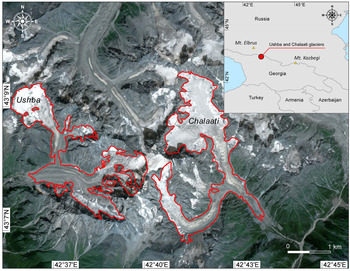
The northern and southern Ushba glaciers have been presented as a single compound-valley glacier since 1960, with an area of ~9.6 km2. The glacier consisted of four tributaries. The two main flows to the left flowed down from the Ushba slopes, and the two flows from the right from the Shkhelda slopes. The glacier has an overall western exposition and terminated at 2400 m a.s.l. Although a recent study by Tielidze (Reference Tielidze and Wheate2017) showed that the compound-valley glacier was divided and presented as two valley glaciers, our SAR approach detected surface movement (over a very narrow path) of debris covered glacier that links the northern and southern Ushba glaciers (Fig. 1). This was also confirmed by a high-resolution SPOT image and recent field investigation. Three medial moraines extend along the ice tongue surface of the southern Ushba Glacier, adjacent to each other on the last part of the glacier tongue and its surface covered by massif debris. The terminal moraines of Ushba Glacier are weakly expressed due to a high ledge. In 2014 data, the glacier terminated at 2600 m a.s.l. (Tielidze, Reference Tielidze and Wheate2017).
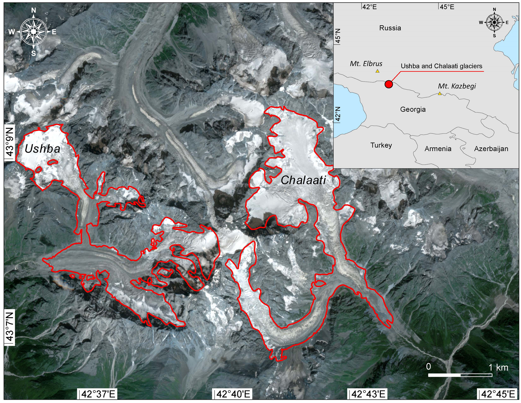
Fig. 1. Sentinel-2 RGB combination images from August 2019, with the boundary of the Ushba Glacier and Chalaati Glacier indicated. Insert map shows the location of Ushba and Chalaati glaciers.
3.2 Chalaati Glacier
Chalaati, located in the Mestiachala river basin on the southern slope of the central Caucasus, is a compound-valley glacier consisting of two tributaries, which are likely to split in the near future (Tielidze and others, Reference Williams, Hall, Sigurdsson and Chien2020b). It is fed from the slopes of peaks, such as Ushba, Chatini, Kavkasi and Bzhedukhi. Among the glaciers of the southern slope of the Caucasus, Chalaati reaches the lowest terminus (1980 m a.s.l. in 2018) and intrudes the forested zone. There are three icefalls in its surface, mimicking the stepped glacier bed. The height of the largest icefall is ~300 m, with a width of ~700 m. In the vicinity of the icefalls, the glacier tongue is rugged due to the various fractures (seracs) of different orientations. The edges of the glacier tongue are covered with debris of variable thickness (Fig. 1). The middle part of the glacier tongue is strongly inclined and cracked. The lateral moraines of Chalaati Glacier are well preserved. At their distal sides they are covered by forest; their proximal sides are bare and steep. The bottom of the valley stabilized in the 20th century, and is now covered by young birch forest. Below ~1750 m a.s.l. there are older moraine walls in conifer forest (Tielidze and others, Reference Williams, Hall, Sigurdsson and Chien2020b).
3.3 Climate
Due to the extreme topographic relief, the study area is characterized by vertical climate zoning. Variations in temperature favor abundant rockfalls, which contribute to covering glacierized surfaces (Negrelli and others, Reference Nigrelli, Fratianni, Zampollo, Turconi and Chiarle2018). According to climate studies carried out the average annual air temperature ranges from −2 to 6°C, decreasing with altitude (Elizbarashvili and others, Reference Elizbarashvili, Samukashvili and Vachnadze2009). In Mestia, the absolute maximum temperature is 38°C, and the absolute minimum temperature is −35°C. The annual precipitation is ~3000 mm. The average decade height of snow cover in winter is 15–55 cm and the maximum height is 1 m.
4. Data and methods
4.1 Data
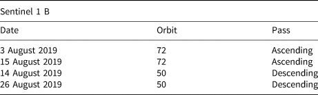
In the current study, Sentinel-1 SAR, Landsat-8 Operational Land Imager (OLI) and Advanced Land Observing Satellite (ALOS) – Phased Array Type L-band Synthetic Aperture Radar (PALSAR) Digital Elevation Model (DEM) data were used to detect debris covered glacierized surfaces. For SAR data, ascending and descending pairs of Single Look Complex (SLC), C-band Sentinel-1B images were used (Table 1). Sentinel-1B, with a 5 × 20 m spatial resolution, was launched on 25 April 2016. The C-band has a wavelength of 5.6 cm. The 30 m-spatial resolution Landsat-8 OLI image (acquisition date: 8 August 2019) was selected to derive the Normalized Difference Vegetation and Snow indices (NDVI and NDSI), detailed below.
Table 1. Orbital characteristics of the SAR images used in the study
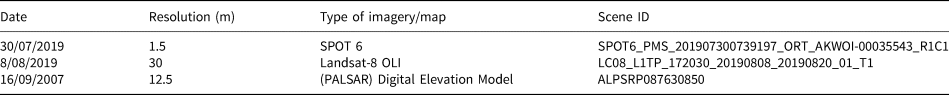
In order to validate our new method with data from the same year, a SPOT 6 satellite image from 2019 was used (Table 2). The glacier outlines from the SPOT image were mapped manually, as was done by Tielidze and others (Reference Tielidze2020a). The Sentinel-1 data were obtained from the Copernicus Open Access Hub (https://scihub.copernicus.eu/), the Landsat satellite images from USGS Earth Explorer (http://earthexplorer.usgs.gov/) and the SPOT data from the Azercosmos facility (https://azercosmos.az/). The ALOS – PALSAR DEM with a resolution of 12.5 m was downloaded from the Alaska Satellite Facility (ASF) Distributed Active Archive Center (DAAC) (https://vertex.daac.asf.alaska.edu) (ASF DAAC, 2015), and was used to generate a slope map.
Table 2. List of the maps, DEM and optical satellite image scenes used in this study
A series of field GPS points were collected from the Ushba Glacier front with a GPS GARMIN eTREX 30x on 8th August 2019. The horizontal accuracy of these GPS measurements varied from 3 to 8 m.
4.2 Methods
DebCovG-carto is an ArcGIS toolbox for the automatic identification of free glacier surfaces and/or supra-glacial deposits, created by us for this study. With the help of this toolbox, radar and optical satellite images are integrated.
4.2.1 Preprocessing of SAR and optical data
Before multi-sensor spatial data can be integrated into DebCovG-carto, the satellite images must be preprocessed (Fig. 2). In this study, Sentinel Application Platform (SNAP) software, freely available from the European Space Agency (ESA), was used to preprocess SAR images and the GLAM-CD toolbox (Holobâcă, Reference Holobâcă2013) to calculate NDVI and NDSI indices.
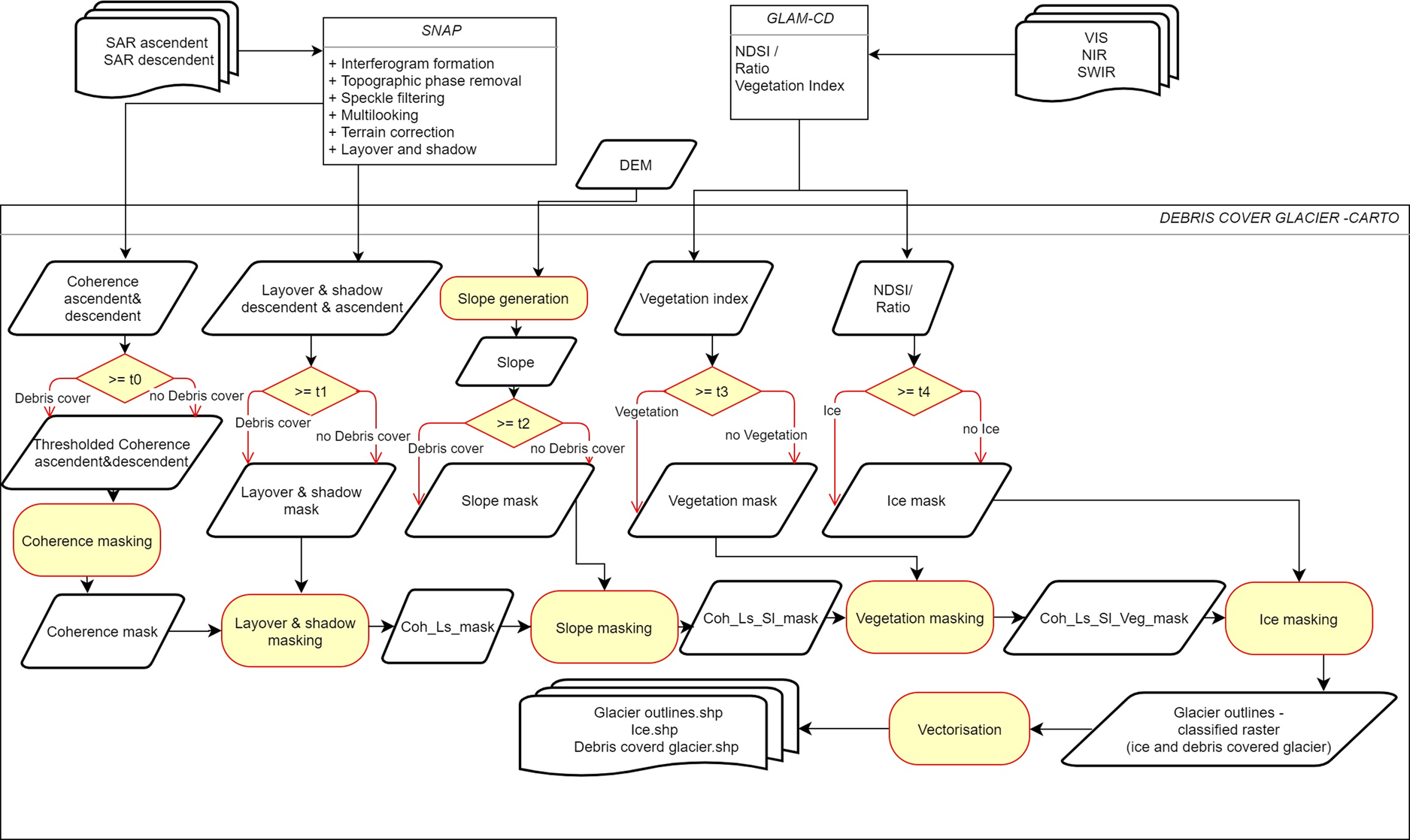
Fig. 2. Multi-sensor remote-sensing data processing chain for debris-covered glacier cartography.
4.2.1.1 Deriving coherence and the layover and shadow mask (SAR):
Two pairs of Sentinel-1 SLC images from the same orbit were used to form the interferogram and coherence images. The Graph Builder tool from SNAP software was used for the automatic calculation process. A predefined graph for SAR interferometry (TOPSAR Coreg Interferogram) was combined with a graph that we defined in order to integrate the SAR interferometry result into DebCovG-carto. This approach allowed us to shorten the processing time by avoiding the step-by-step algorithm.
The TOPSAR Coreg Interferogram graph allows a debursted interferogram to be obtained for a sub-swath. Before generating the interferogram, the Sentinel-1 SLC split pairs (primary and secondary) of the sub-swath are co-registered using the orbits of the two products and a DEM. This geometric correction is essential for calculating the interferogram. Finally, the results are debursted (re-sampled to a common pixel spacing grid in range and azimuth).
The result was then prepared for integration into the DebCovG-carto toolbox. The topographic phase was subtracted from the interferogram (the DEM was first ‘radar coded’ to the area of the interferogram, and was then subtracted from the complex interferogram). Speckle noise, inherent in an SLC image, was reduced using Goldstein Phase Filtering (Goldstein and Werner, Reference Goldstein and Werner1998) and Multilook Method (which, in addition to reducing noise, also produces square ground pixels). The final SNAP processing step is the Range Doppler Terrain Correction.
The SAR Simulation Terrain Correction Operator is used to create the layover and shadow mask. This operation is necessary because the layover effect causes the signal backscattered from the top of the mountain to be received earlier than the signal from the bottom (causing the fore slope to be inverted). The shadow effect completely masks the information from the backslope.
4.2.1.2 Deriving NDSI and NDVI:
In the current study, we employed the GLAM-CD toolbox to calculate the optical satellite indices used to build ice and vegetation masks. For both indices, a normalized difference was calculated in order to enhance the variation in the slope of the spectral reflectance curves between two different spectral ranges. Snow and vegetation strongly reflect visible light (VIS; e.g. green and red), but absorb SWIR (e.g. ice) or NIR (e.g. vegetation) light. The satellite index values are high over snow and ice (NDSI) and over vegetation (NDVI).
4.2.2 DebCovG-carto algorithm
We developed an approach (DebCovG-carto) to map debris using ascending and descending SAR pairs and the coherence maps that result from ice motion between the acquisitions. The main challenge for debris-covered glacierized surface detection using coherence images is to keep only the coherence loss due to ice displacement (moving surfaces). According to the ESA RADAR and SAR glossary https://earth.esa.int/handbooks/asar/CNTR5-2.html#eph.asar.gloss.radsar:INTERFEROMETRY: ‘In an interferogram, coherence is a measure of correlation. It ranges from 0.0, where there is no useful information in the interferogram; to 1.0, where there is no noise in the interferogram (a perfect interferogram)’. The decorrelation between two SAR images is caused by: slope (steep slopes have low coherence because of low signal-to-noise ratio; Massom and Lubin, Reference Massom and Lubin2006), vegetated surfaces (decorrelation caused by volume scattering – multiple scattering events take place when electromagnetic wave is inside a medium containing scatterers with discrete dielectric properties; Zebker and others, Reference Zemp2007), baseline (large baselines lead to low coherence; Li and Goldstein, Reference Li and Goldstein1990), time lag between images (long lags lead to low coherence; Zebker and Villasenor, Reference Zebker, Shankar and Hooper1992) and generation of the interferogram (poor co-registration or bad resampling). On a glacier surface, a substantial change in the glacier surface (glacier surge, substantial melt or snowfall) can lead to low coherence. Some of these problems can be solved through the correct choice of season and SAR images used, and, if available, the consultation of meteorological data.
The highest coherence values are observed at the peak of the ablation season (July–August) (Lu and Freymueller, Reference Lu and Freymueller1998). The minimum time lag when using descending and ascending pairs for Sentinel-1 is controlled by the 12-day repeat orbit cycle. This time lag is sufficient to capture the movement of ice, and at the same time does not generate a major loss of coherence for other land-use classes. The use of ESA-corrected products (SLC level 1) and SNAP preprocessing algorithms can significantly reduce interferogram generation errors.
The DebCovG-carto algorithm uses coherence images derived from ascending and descending pairs of SLC, C-band, Sentinel-1 images to map the debris-covered part of mountain glaciers:
(1) Coherence thresholding: in the first step of the algorithm, a threshold (t 0 = 0.3) is applied to the two coherence images. Thus, only surfaces with a coherence of <0.3 are preserved. For threshold detection, we used a gradient descent algorithm with a step of 0.01 (Henstock and Chelberg, Reference Henstock and Chelberg1996). This value was found to result in the best separation of the debris-covered glacierized surfaces.
(2) Coherence masking: the two coherence images to which the t 0 threshold was applied are integrated.
(3) Layover and shadow masking: in this step, the areas that have low coherence due to the layover and shadow effects are removed from the coherence mask.
(4) Slope masking: an external DEM is used to build the slope map. It is reclassified using a threshold value (t 2). In this study, we used the value of 30° to mask those pixels with low coherence values on the mask obtained in the previous step.
(5) Vegetation masking: from the comparisons made using NDVI values and coherence images, a threshold of 0.2–0.3 (moderate values represent shrub and grassland) was observed, which, if exceeded, produces a significant decrease in the coherence of the analyzed images. In this context, all the pixels that had a coherence below the t 0 threshold and an NDVI value (t 3) >0.3 were masked in the raster obtained in the previous step.
(6) Ice masking: in this step, pixels that are covered with snow or ice are also masked. A threshold (t 4) is applied to the NDSI image, the value of which is 0.4 in this study, and pixels with a value higher than this threshold are classified as surfaces covered by snow or ice. Thus, the ‘glacier outlines’ raster is obtained with two classes: debris-covered glacier and ice-covered glacier.
(7) Vectorization: in the final step of the algorithm, three categories of glacier outline are obtained by vectorization (debris-covered glacier area, ice-covered glacier area and glacier outlines (i.e. total glacierized area)). For the vectorization step, we used the Raster to vector tool from ArcGis9. The raster obtained in the previous step and, optionally, an external reference limit (owner, national inventory, international database: GLIMS, RGI, etc.) are used in this step. The outlines can be exported in KML format and opened using a KML reader such as Google Earth or KML viewer for quick visual validation and manual correction.
5. Results and discussion
5.1. DebCovG-carto algorithm output
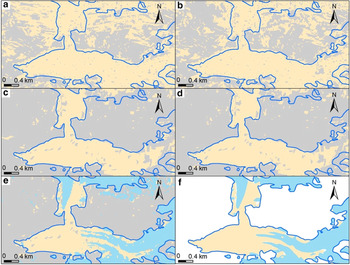
Combining the coherence information contained in the two images with data from ascending and descending passes is essential for high-quality debris-covered surface mapping. This improvement can especially be seen around the glacier front and the contact areas with the slopes. A side effect is the reduction of the speckle effect, characteristic of radar images. The speckle model is different in the two images, and is considerably reduced when the two images are combined in the first step of the DebCovG-carto algorithm (Fig. 3a). When using a single coherence image derived from an ascending or descending satellite image, the area of the detected supra-glacial deposit is substantially smaller (~15% in the case of the Ushba Glacier). This reduction is due to the speckle phenomenon characteristic of radar images, the different perspective of the antenna in the ascending and descending passage and layover shadow which therefore appear only on one of the two images.
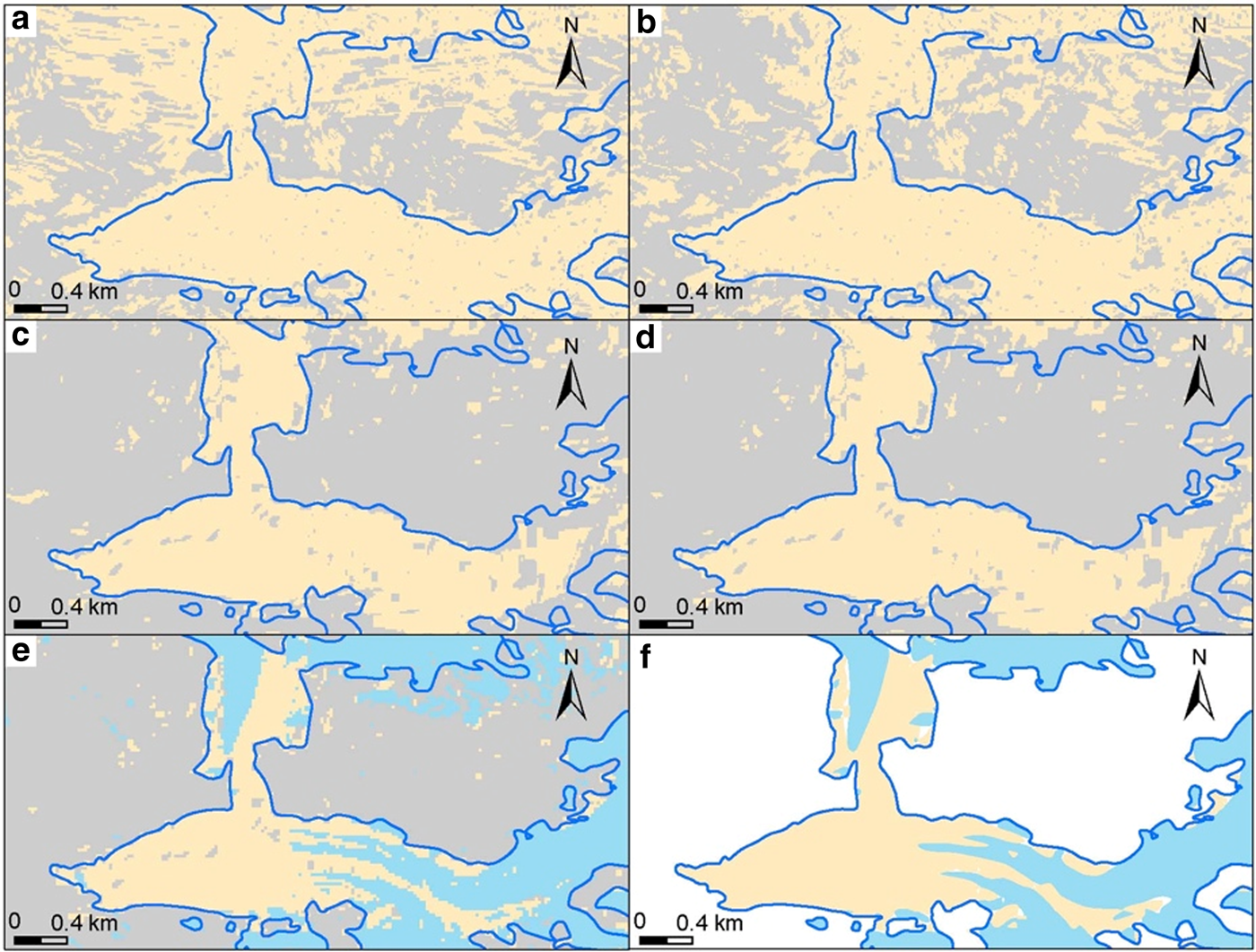
Fig. 3. Extraction of debris-covered and snow-/ice-covered outlines for Ushba Glacier (f) using the step-wise masking of the DebCovG-carto algorithm (a–e): a – coherence masking; b – layover and shadow masking; c – slope masking; d – vegetation masking; e – ice masking; f – vectorization.
Similarly, due to the different geometric properties of the images in the ascending and descending orbits, the layover and shadow areas are different in the two pairs of images. The use of complementary images makes it possible to retrieve information from the layover or shadow areas if in one of the two images the respective area is not affected (Fig. 3b).
The next step, slope masking, has the greatest impact on masking areas that do not correspond to debris-covered glacierized surfaces. The result obtained at this step integrates the influence of the relief parameters on the glacier processes and on the coherence of the SAR images (Fig. 3c).
The vegetation mask, which we propose for the first time in this study, is necessary if the glacier front is located below the upper altitudinal vegetation limit. In our case, the fronts of Ushba and Chalaati glaciers (as for many other glaciers in the Caucasus and around the world) are below this limit. At this stage, a large part of the area below the glacier front and on the side and slopes is filtered (Fig. 3d).
If the coherence value of a pixel in the previous steps is not due to the movement of the debris-covered glacierized surface have been removed, now the snow-covered or ice-covered pixels are added (Fig. 3e). DebCovG-carto, compared to other methods that are usually specialized, offers the possibility to classify both snow- and ice-covered surfaces and debris-covered glacierized surfaces.
Three categories of surfaces were obtained through vectorization: the total glacierized surface, the surface covered by snow and ice and the debris-covered glacierized surface (Fig. 4). These can then be used to extract information related to glacier processes and to update the glacier inventories for multi-temporal analysis.
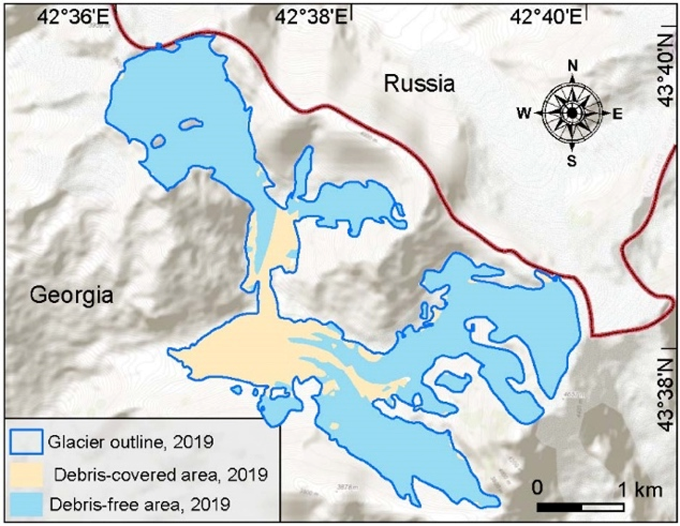
Fig. 4. Ushba Glacier outlines obtained using DebCovG-carto.
5.2 Validation of SAR results with field measurements and SPOT imagery
Validation of the method was performed using field GPS points and the 2019 SPOT-derived glacier boundary. The GPS points taken in the field were used to validate the position of the glacier front and cross-validation analysis was performed on the debris-covered area.
5.2.1 The Ushba Glacier front
This was validated using the GPS points from the field taken on 8 August 2019. The boundary drawn using these confirms the position determined using DebCovG-carto. The differences between the two are minor and do not exceed the size of two pixels (30 m). For front detection, the SAR method performed better than the manual approach (Fig. 5).
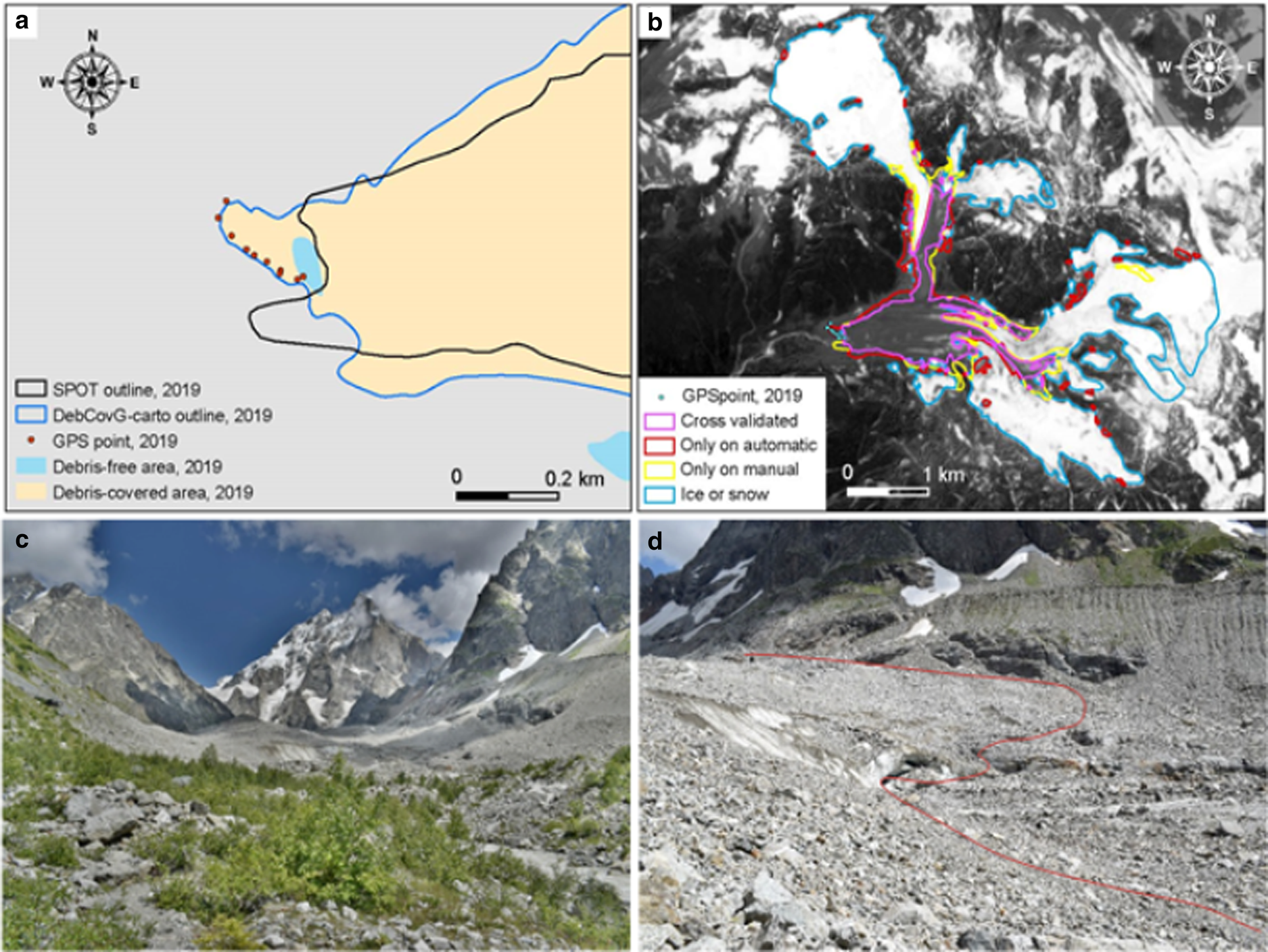
Fig. 5. Validation of the results for Ushba Glacier: (a) front validation using GPS points from the field taken on 8 August 2019; (b) cross-validation between automatic and manual methods; (c) front and next-to-front debris-covered area and (d) glacier front (red line) of Ushba Glacier (photos from 8 August 2019).
5.2.2 Cross-validation of the debris-covered area
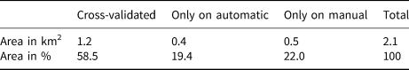
The differences between the limit obtained for 2019 using the manual method and the limit determined automatically for 2019 were identified using the change detection module in the GLAM-CD toolbox. Surfaces that were classified in the same class using both the automatic and the manual methods were considered cross-validated. Cross-validation was successful for almost 60% of the surface (Table 3). If we compare the limits obtained using the two methods, the automatic method extends more toward the slopes than the one obtained manually. Thus, 19.4% of the validation surface appears only for the automatic method. An almost equal proportion (22.0%) appears only in the manually-drawn limit, which performed better on the steep parts of the glacier (Table 3).
Table 3. Cross-validation of the debris-covered area using automatic and manual data, Ushba Glacier
5.2.3 External validation
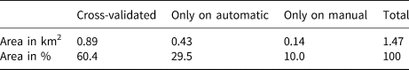
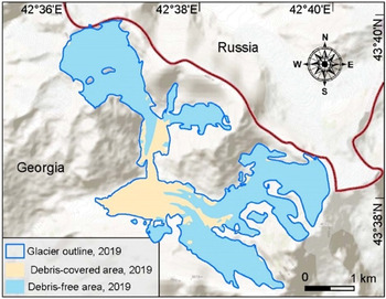
The automatic method was also applied to the Chalaati Glacier in order to validate the results obtained using the DebCovG-carto toolbox. This glacier was chosen because its front part was explored and mapped in August 2019. Also, a debris-covered surface delimitation was available in 2019 from an independent source (Tielidze and others, Reference Williams, Hall, Sigurdsson and Chien2020b). Moreover, the difference in general orientation of theses glacier systems, from east to west for Ushba Glacier and from north to south for Chalaati Glacier (Fig. 6), may impact the accuracy of the satellite antenna, which is oriented toward the glacier surface. In this regard, the comparison and spatial analysis of both glaciers were also useful.
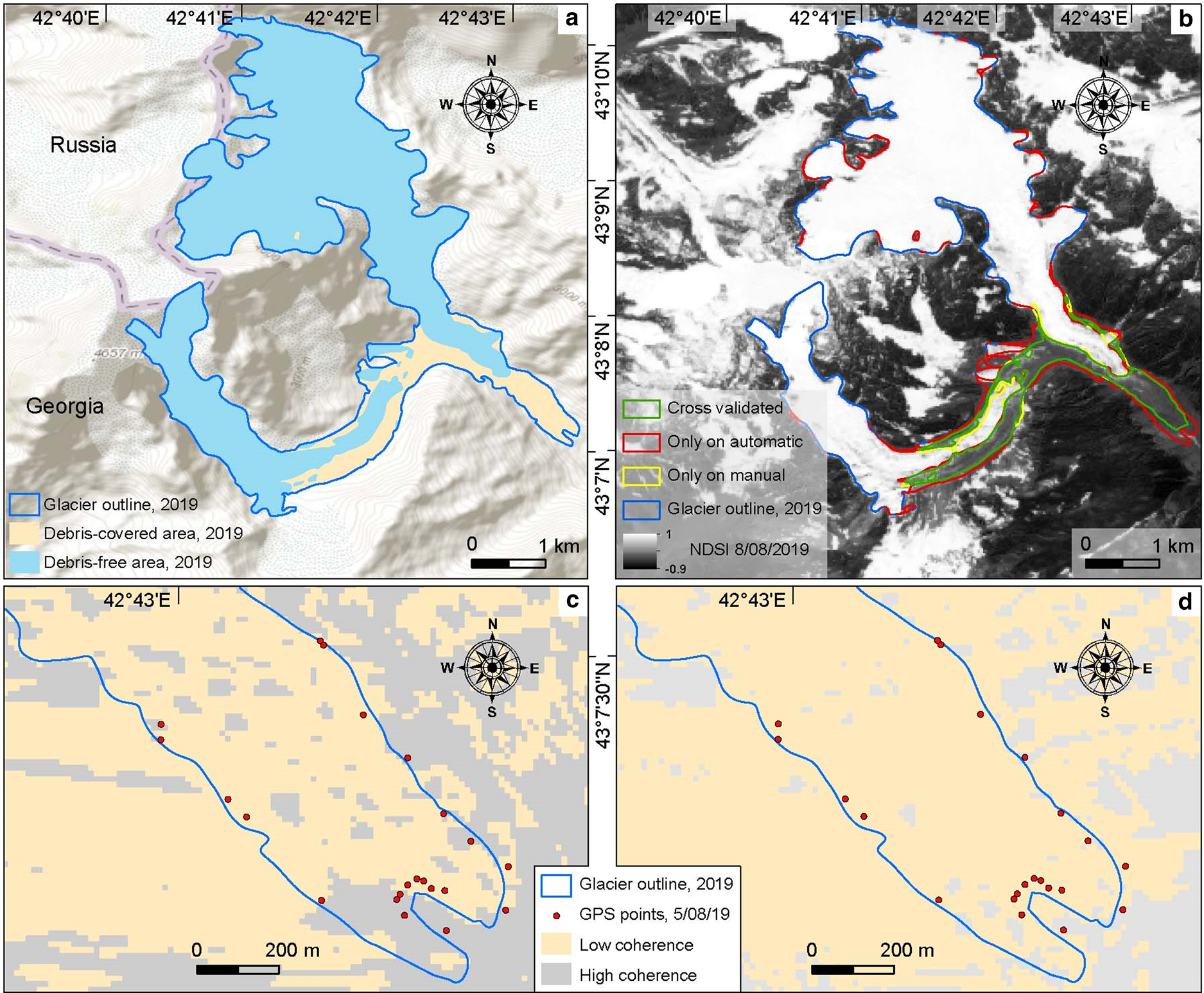
Fig. 6. Validation of the results for Chalaati Glacier: (a) Chalaati Glacier outlines obtained using DebCovG-carto; (b) cross-validation between automatic and manual methods; (c) coherence on descending image and (d) coherence on ascending image.
In the frontal area of the Chalaati Glacier, the differences between the automatically-obtained limits and the GPS points taken in the field did not exceed 2 pixels (30 m), results similar to those previously obtained for Ushba Glacier. Good results were also obtained for the contact with off-glacier taluses when compared with field GPS points, especially on the left side of the debris-covered area, which was more accessible (Fig. 5). The major difference between the two methods seems to appear in this area. Indeed, the automatic method also detects debris-covered glacial surfaces in the accumulation area. This makes the area classified as covered by debris larger than that in the case of the manual method (Table 4). However, the percentage of surface classified as debris-covered by both methods appears to be quite similar (60.4%).
Table 4. Cross-validation of the debris-covered area using automatic and manual data, Chalaati Glacier
Because at this time the automatic method indicates a loss of coherence that can be attributed to other causes of glacier movement, while the manual method is based on a very good knowledge of the glacierized area (field observations and measurements), we cannot precisely estimate the source of the error.
Despite the presence of extensive supra-glacial deposits in the Greater Caucasus (Tielidze and others, Reference Tielidze2020a), the potential of using SAR to delineate these regions has not been exploited to date there. This study is the first attempt to use this technique in this region. In the past, access to SAR satellite imagery was difficult and expensive, and processing was very difficult. The use of radar satellite images is now more user-friendly since the development of SAR processing methodology and software and especially since ESA has provided unrestricted access to its archive.
The main novelty contributed by the algorithm presented in this study compared to previous studies using coherence images to identify debris coverage of glacierized surfaces (Jiang and others, Reference Jiang, Liu, Wang, Lin and Long2011; Lippl and others, Reference Lippl, Vijay and Braun2018) is the integration of coherence images calculated from two pairs of images from identical orbits (ascending and descending).
The different orientation of the antenna and the complementary geometric characteristics provide different perspectives on the analyzed glacierized surfaces leading to:
(1) Considerable improvement in mapping of the frontal area and of the contact with the slopes by combining the two images. This is notable in the case of Ushba Glacier, which has a steep front (Fig. 7c).
(2) The possibility of recovering information that is in layover or shadow if the effect is present in only one of the two images (Fig. 8c).
(3) The considerable reduction of the speckle effect characteristic of SAR due to the different model applied to the two images. This technique has eliminated the filtering that is commonly used in SAR image processing. The use of morphological filters to eliminate the mirror effect can lead to a loss of information through resampling.
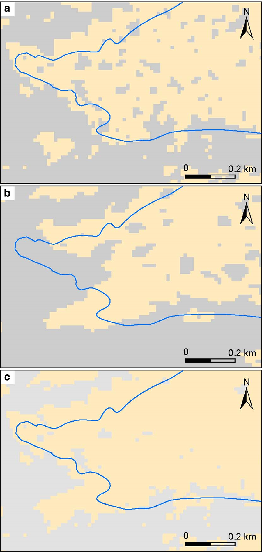
Fig. 7. Improvement of the front detection and speckle reduction by integration of the complementary coherence images: (a) coherence on descending image; (b) coherence on ascending image; (c) coherence on integrated image (blue line – Ushba Glacier outlines 2019; beige area – coherence below threshold t 0).
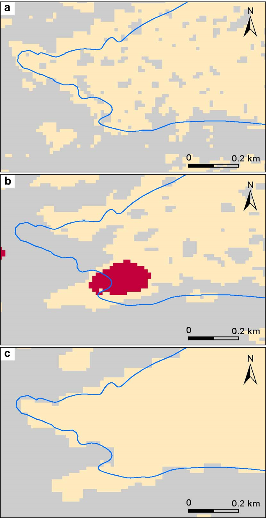
Fig. 8. Recovery of information that is in layover or shadow in the ascending image in the frontal area of Ushba Glacier: (a) coherence on descending image (no layover or shadow); (b) coherence and shadow on ascending image; (c) coherence after layover and shadow mask (blue line – Ushba Glacier outlines 2019; red area – layover or shadow; beige area – coherence below threshold t 0).
Another novel aspect of this study is the vegetation masking. From the analysis carried out here, a significant reduction in the coherence at high NDVI values was observed. A potentially very useful application of this mask is the discrimination coherence loss due to the movement of debris-covered ice surfaces from that due to the presence of vegetation on the moraine deposits.
The DebCovG-carto toolbox makes automatic mapping of glacierized surfaces considerably faster than the use of subjective methods (Hall and others, Reference Hall, Williams and Bayr1992; Bayr and others, Reference Bayr, Hall and Kovalick1994; Paul, Reference Paul2002a, Reference Paul2002b). The results obtained using this algorithm thus have great potential to be used for large-scale studies that require the processing and interpretation of a large volume of spatial data. The combined use of the new toolbox and GLAM-CD makes it possible to simultaneously extract information about the local-scale properties of both debris-covered and debris-free glacierized surfaces.
Based on glacier front mapping carried out in the field for validation, the accuracy of the method is estimated to be 2 pixels, or 30 m. The error related mainly to mixed pixels. The cross-validation analyses show that the complementary use of the SAR automatic method with a manual approach performed by an experienced operator can significantly improve the accuracy of debris-covered glacier detection, offering the analyst objective information (debris-covered glacierized movement) to better identify the contact with off-glacier talus.
The limitations of the method are related to the challenges associated with the use of SAR images in mountainous areas. The presence of strongly-fragmented relief led to the presence of areas with low coherence values on steep slopes or in the areas situated in layover or shadow. These areas cannot be classified as debris-covered glacierized surfaces and require further analysis using other investigative methods. Due to the use of two pairs of SAR images in our approach, the loss of information from layover and shadow is considerably reduced. At the same time, debris deposits are limited on steep slopes of the glacierized surfaces and are considerably more common on moderate slopes, where detection using our method is possible.
Another limitation of this method is the application only on two sets of SAR imagery. The analysis of multiannual images will be difficult due to the increased melting rates of the Caucasus glaciers (especially, the high loss of the frontal area), e.g. Tielidze and others (Reference Williams, Hall, Sigurdsson and Chien2020b) measured almost 3 km retreat of Chalaati Glacier in 2000–2018 and this (retreat rate) is likely much higher between 2017 and 2020.
The uncertainty that vectorization adds to the delineation of the glacier is relatively low. The difference between the vector- and raster-based glacial surface calculation is 0.23% for the Ushba Glacier and 0.34% for Chalaati Glacier.
6. Conclusions
We successfully identified regions of debris-covered ice at two glaciers in the Greater Caucasus Mountains using SAR and optical satellite imagery. Our approach reduces processing time and mapping error, demonstrating the promise this technique holds for broader scale glacier outline mapping. The use of SAR-based methods that detect glacier debris-covered surface movement reduces the processing time and mapping error.
The main finding of this study is the improvement of debris-covered glacier surface detection using pairs of SAR images from ascending and descending orbits. Our approach enhances outline detection in the most problematic areas including glacier termini and slope contacts. It also improves information recovery from layover and shadow areas, and considerably reduces SAR speckle. We also developed a vegetation mask that removes volume scattering decorrelation caused by vegetation. Future study will focus on improving this algorithm.
Our study using DebCovG-carto documents the substantial retreat and mass loss ongoing in the Caucasus region. Better constraints on ice loss are needed for predicting water availability for irrigation and hydropower. Millions of people depend on meltwater from these glaciers, and the retreat and loss of glacier mass will lead to important social and economic consequences in the future.
The DebCovG-carto tool will be available on GitHUB for the scientific community to test in other geographic areas and on other C, L or X band datasets. Data other than Sentinel-1 can be integrated directly into the algorithm after obtaining the coherence product, provided that their projection and resolution are consistent with the other products used by the algorithm, such as the DEM.
Data
The data that support the findings of this study are available on GitHUB (https://github.com/iulianholo/DebCov_Carto).
Acknowledgements
This study was supported by Projets de Recherche Conjoints AUF – IFA 2018, 08 AUF: Impact du changement climatique sur les glaciers et les risques associés dans le Caucase (IMPCLIM) and by Babeș-Bolyai University Centenar dedicated activities. We thank Dr Roger Wheate for the final language check.
Author contributions
H.I.H. conducted field research, developed the DebCovG-carto methodology and conceived and wrote the manuscript; L.G.T. contributed to the general introduction, methodology and data analysis, and also provided topographic and satellite data; K.T.-I. participated in field research and elaboration of the cartographic materials; M.E. wrote the study area description; M.A. filled in glacier front cartography and prepared the manuscript; D.G. revised English language and scientific terminology; S.H.P. participated in fieldwork and photography; O.T.P. revised the study area information; G.G. wrote the study area description.
Financial support
The publication of this paper was supported by the 2020 Development Fund of the Babeș-Bolyai University.
Conflict of interest
The authors declare no conflict of interest.


 Open access