
Abstract
We investigated the appropriateness of a tunneling magnetoresistance (TMR)-based magnetometer for detecting geomagnetic fields with long-period oscillations through observation of the geomagnetic pulsation (Pi). Pi was not sufficiently observed in the raw outputs due to thermal noise; a bandwidth-limitation treatment helped extract Pi without data stacking. The detectable intensity was reduced to 1 nT with a period of 30 s, but detection was impossible for 100 s. The frequency characteristics revealed that reducing the cutoff frequency of a TMR magnetometer is a promising approach for detecting field oscillations occurring over long periods, such as 100 s.
Export citation and abstract BibTeX RIS

Content from this work may be used under the terms of the Creative Commons Attribution 4.0 licence. Any further distribution of this work must maintain attribution to the author(s) and the title of the work, journal citation and DOI.
An earthquake due to the release of stress in rocks and/or faults is one of the mechanisms that induces a change in the local geomagnetic field through the piezomagnetic effect. 1–5) The signal associated with such a change in the geomagnetic field propagates at the speed of light from the epicenter of the Earthquake and can be detected far earlier than the arrival of seismic waves. Hence, detection of such changes in the geomagnetic field could potentially serve as a "super-early warning system" for destructive earthquakes, which would be considerably faster than conventional warning systems. Therefore, long-term observation that can help establish a novel warning system is necessary from the perspective of disaster prevention. For example, we previously reported a clear increase in the geomagnetic field by ∼300 pT several seconds prior to the "Iwate–Miyagi Nairiku" earthquake using a flux-gate magnetometer (hereinafter referred to as "FG"). 5) H. Utada, et al., reported on the geomagnetic field change in response to the 2011 Tohoku-oki earthquake, including the tsunamigenic electromagnetic disturbances. 6) The time for changes in the geomagnetic field is generally proportional to the duration of crash in faults, considering the piezomagnetic effect: a time scale of 100 s would be considered for significantly large fault length in cases such as off-shore earthquakes, while several tens of seconds would be considered in the case of inland earthquakes. 7) This indicates that magnetometers need to be highly sensitive to geomagnetic fields for long periods such as 1–100 s to detect changes in these fields due to various earthquakes. We have further employed a superconducting quantum interference device magnetometer (SQ) and have reported its significant potential to detect even small changes in the geomagnetic field, which is the result of a higher sensitivity compared with that of the conventional FG. 8) However, the SQ has not been commercialized, because of its expensive components and the high running costs associated with the regular supply of liquid nitrogen required.
In this context, tunneling magnetoresistance (TMR)-based magnetometers have recently attracted considerable attention. TMR magnetometers consist of magnetic tunnel junctions (MTJs),
9,10) which have been developed for spintronic devices such as reading heads of hard disk drives with a high TMR ratio and low resistance area product
11–13) and magnetic random access memories.
14,15) In the most recent studies, Fujiwara et al. demonstrated the sensing of low bio-magnetic fields, such as magnetocardiography and magnetoencephalography signals, using TMR sensors.
16–18) This accomplishment can be attributed to the high sensitivity of TMR sensors (4 pT/ at 1 Hz),
19) which is similar to or higher than that of the representative FG (4–10 pT/
at 1 Hz),
19) which is similar to or higher than that of the representative FG (4–10 pT/ at 1 Hz).
20) The sensitivity of TMR magnetometers is reliable for the oscillation period of bio-magnetic fields (∼50 ms based on the peak-to-peak time of magnetocardiography oscillations, as shown by Fujiwara et al.
18)); however, it remains unclear how the aforementioned sensitivity of 4 pT/
at 1 Hz).
20) The sensitivity of TMR magnetometers is reliable for the oscillation period of bio-magnetic fields (∼50 ms based on the peak-to-peak time of magnetocardiography oscillations, as shown by Fujiwara et al.
18)); however, it remains unclear how the aforementioned sensitivity of 4 pT/ at 1 Hz and/or the reliability of TMR sensors change at less than 0.1 Hz. With regard to TMR sensors, neither has such a reliability at lower frequency regime been investigated, nor has outdoor operation with long-term and continuous observation been performed. Therefore, demonstrations are required to determine the appropriateness of TMR magnetometers for detecting geomagnetic fields exhibiting long-period oscillation.
It is difficult to predict when and where an earthquake will occur. Therefore, we focus on global changes in geomagnetic fields, that is, geomagnetic pulsations (Pi). The characteristics of Pi are well-known, 21–24) which has been widely used as a standard signal for calibrating various magnetometers. Pi oscillates with a period of 1–150 s and has an amplitude intensity of ∼10 nT; 22) these values are similar to the time scale and the amplitude of geomagnetic field variations caused by earthquakes. 5) Therefore, the appropriateness of TMR magnetometers for the detection of geomagnetic fields exhibiting long-period oscillations was investigated through observation of Pi in this study. The results confirm the feasibility of applying bandwidth-limitation treatment to raw outputs, and the minimum detectivity was found to be 1 nT with a period of 30 s.
Figure 1(a) shows a map of Fukushima-ken, where a TMR magnetometer was placed at the geomagnetic field observatory in Iwaki (IWK) city. The location of the Kakioka (KAK) observatory in Ibaraki-ken, where standard geomagnetic field monitoring is performed by the Japan Meteorological Agency, is also shown on the same map. Figure 1(b) shows the layout of the IWK observatory, in which the FG, SQ, and TMR magnetometers are placed to enable multiple observations. Owing to the multiple observations, the data from the TMR magnetometer can be compared with those from the FG and SQ. The IWK observatory is located on a field surrounded by grass and is situated far from downtown Iwaki to observe pure Pi components. Furthermore, the magnetometers do not interfere with each other because of the distances at which they are placed. Figure 1(c) shows a box, in which the TMR sensor with a flux-concentrator (FC) and pre-amplifier were fixed, to avoid rain and wind from affecting the observations. The box was fixed on the ground and covered with an aluminum sheet to prevent any increase in its surface temperature.

Fig. 1. (Color online) (a) Map showing the Iwaki (IWK) city observatory, where the TMR magnetometer is placed, along with the Kakioka (KAK) observatory, which is a standard geomagnetic observatory operated by the Japan Meteorological Agency. (b) Layouts of the TMR, flux-gate (FG), and squid (SQ) magnetometers in the IWK observatory. (c) Image of box with TMR sensor module and flux concentrator.
Download figure:
Standard image High-resolution imageFigure 2(a) shows a block diagram of the TMR magnetometer with the FC and data-recording systems. The high- and low-pass filters (0.01–10 Hz), and pre- and main amplifiers (60 and 60 dB) were the same as those of the TMR magnetometer for bio-magnetic field sensing (Spin Sensing Factory, Inc.). Owing to the use of the band-pass filters, the temperature-driven output change could be eliminated. The FC was made of Fe-based alloy foils with a thickness of 18 μm and was placed near the MTJ-arrayed sensors. The main amplifier with an arrester and the recording systems with a power source were connected using 30 m electric coaxial cables to prevent the geomagnetic field from generating disturbances at the recording systems and/or devices. With this system, 32 bit data recording was continuously performed at a sampling rate of 50 Hz for ten months. Figure 2(b) shows bridge circuits with four MTJ-arrayed sensors together with the pre-amplifier, which corresponds to the part denoted by the dashed circle in Fig. 2(a). Since the size of the sensor bridge was around 2 cm, a large FC was needed to supply a uniform magnetic field to the bridge [Fig. 2(a)], and the sensitivity enhancement was designed to be 8 times (although the actual enhancement is unknown here). One MTJ array comprising many MTJs connected in series and parallel was used to reduce the noise level. The red arrow for each MTJ represents the magnetization direction of the free layer; as can be seen, all the arrows point in the same direction. The large red arrows for the bridge indicate the total magnetization direction of the free layer for the MTJ array. Figure 2(c) shows a schematic illustration of a representative MTJ. The magnetic easy axis of the free layer of the MTJ is orthogonal to that of the pinned layer; hence, a linear output could be obtained depending on the external magnetic field. The most sensitive axis of the MTJ, corresponding to the magnetic hard axis of the free layer of the MTJs, is aligned northward, where the largest variation in geomagnetic fields can be expected. The frequency-dependent sensitivity of the TMR magnetometer without the FC was evaluated using a laboratory-based magnetic coil and oscilloscope and was determined to be 500 mV nT−1 at 4 Hz. The noise spectral density (NSD) of the entire magnetometer with the FC was evaluated at the IWK observatory. Note that data stacking was not allowed for the observation and analysis, because real-time monitoring is essential for studying geomagnetic fields. The full range of the signal voltage from the main amplifier was adjusted to be ±10 V.
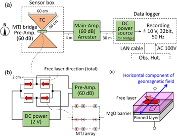
Fig. 2. (Color online) (a), (b) Block diagrams of entire TMR magnetometer (a), and bridge circuits of four MTJ-arrays with pre-amplifier (b). The MTJ-array consists of many MTJs connected in series and parallel. The red arrows represent the magnetization direction of the free layer. (c) Magnetization configuration of one MTJ together with the field direction detected by the MTJ.
Download figure:
Standard image High-resolution imageFigures 3(a-1)–3(c-1) show the raw geomagnetic field and raw output voltage observed using the two FGs and the TMR magnetometer, respectively. The output voltage for the TMR magnetometer is shown because no calibration was performed from voltage to field. The data from the FG in the KAK observatory are also shown. 25) The geomagnetic signal shown here corresponds to the field in the northward direction and is the same as that for the TMR magnetometer. In the case of the two FGs, clear oscillations with a period of several 10 s could be observed during the long and gradual change in the geomagnetic fields. These clear oscillations correspond to Pi signals, which were the focus of this study. The data from the FG at the IWK observatory agreed well with the data recorded at the KAK observatory; this suggests that the Pi samples observed in IWK were appropriate as a global geomagnetic signal. Table I summarizes the three samples of Pi used to identify the characteristics of the TMR magnetometer. Samples A and B have similar period features but different field intensities, whereas samples A and C have similar field intensities but different period features. The period represents the time between two successive peaks for the representative Pi oscillation indicated by the arrows in Figs. 3(a-1)–3(c-3).
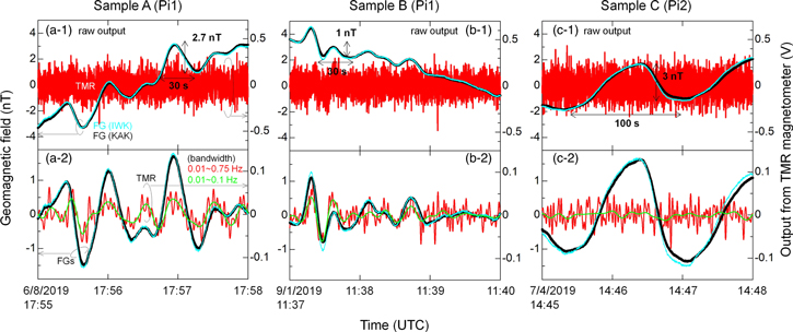
Fig. 3. (Color online) (a)–(c) Geomagnetic field and output voltage observed by the FGs and TMR magnetometer, respectively. The top and bottom images present the results with [(a-c)-1] and without [(a-c)-2] bandwidth limitation treatment (0.01–0.75 Hz and 0.01–0.1 Hz), respectively.
Download figure:
Standard image High-resolution imageTable I. Pi samples investigated and shown in Fig. 3. The Pi classification is based on Ref. 22.
| Samples | Classification | Time (UTC) | Peak-to-peak intensity | Period |
|---|---|---|---|---|
| Sample A | Pi1 | 6/8/2019 | 2.7 nT | 30 s |
| Figure 3(a) | 17:55–17:58 | |||
| Sample B | Pi1 | 9/1/2019 | 1 nT | 30 s |
| Figure 3(b) | 11:37–11:40 | |||
| Sample C | Pi2 | 7/4/2019 | 3 nT | 100 s |
| Figure 3(c) | 14:45–14:48 |
In contrast to that from the two FGs, the raw output voltage from the TMR magnetometer was almost 0 and exhibited no evident peaks associated with the Pi signal for any of the samples. This difference between the FGs and the TMR magnetometer was due to the effect of the nominal band-pass filters: FGs and TMR magnetometers can measure frequencies of DC ∼5 Hz and 0.01–10 Hz, respectively. The results indicate that the near-DC component dominates the Pi signal, which might be one of the reasons for no Pi signals appearing in the raw output of the TMR magnetometer. Another factor to be considered is the larger thermal disturbance noise compared with the Pi signal amplitude for the TMR magnetometer. These findings led us to conduct an appropriate data analysis to extract the Pi signals from the raw output. We applied bandwidth limitation to the raw output. Figures 3(a-2)–3(c-2) show the results of applying bandwidth limitations of 0.01–0.75 Hz (red) and 0.01–0.1 Hz (green), where 0.01 Hz is the nominal frequency of the band-pass filters in the TMR magnetometer. Compared with that in the case of 0.01–0.75 Hz, higher-frequency noise in the case of 0.01–0.1 Hz was reduced owing to the narrower bandwidth available for all samples. Here, the slope of the base line corresponding to the long-term trend of the geomagnetic field observed by the FGs was excluded from the raw data of the FGs to enable comparison with the results yielded by the TMR magnetometer. The Pi signals from the TMR magnetometer for both bandwidths could be detected, and the period was consistent with that observed by the FGs, as shown in Figs. 3(a) and 3(b). These results show that the use of raw output signals for real-time observation is not preferable for the studied TMR magnetometer; this might be because the nominal cutoff frequency as well as the thermal noise exceeded the Pi intensity. Therefore, it was revealed that bandwidth limitation is one of the necessary treatments for observing Pi signals when using TMR magnetometers. To investigate the lowest output that the TMR magnetometer can detect, we compared two Pi samples, A and B, with similar periods. Based on the results, the TMR magnetometer could detect Pi signals as weak as 1 nT [Fig. 3(b)], suggesting good detectivity of the geomagnetic field changes before the arrival of earthquakes. Subsequently, to investigate the period dependence of Pi signal detection, we compared two Pi samples, A and C, with similar field intensities. Sample C, with a period of 100 s, could not be detected, even though its intensity of 3 nT is much higher than the minimum detection limit of 1 nT. We also attempted to impose a greater bandwidth limitation of 0.01–0.1 Hz to focus on lower frequency signals, however, Pi signals oscillating with a period of 100 s were not detected. This result shows that the signal sensitivity of the studied TMR magnetometer varies with frequency. Therefore, the frequency-dependent sensitivity of the studied TMR magnetometer was evaluated for discussion.
Figure 4(a) shows the NSD of the FGs and the TMR magnetometers with an FC, as determined at the IWK observatory. Data stacking was performed to broaden any specific geomagnetic signals such as Pi. Therefore, Fig. 3(a) shows the NSD for the entire FGs and TMR magnetometers. Although the NSD of the FGs increased with decreasing frequency due to the absence of a DC cut filter, a sensitivity of 6 pT/ at 1 Hz was confirmed. By contrast, the NSD of the TMR magnetometer decreased remarkably in the <0.01 Hz regime because of the analog high-pass filter. Such a low NSD at lower frequencies might be preferable in the case of fields with long-period oscillation. However, the frequency dependence of the sensitivity of the studied TMR magnetometer must be considered as well.

Fig. 4. (Color online) (a) Noise spectral density of the FG and TMR magnetometers observed at IWK observatory. (b) Frequency dependence of signal sensitivity of the TMR magnetometer (without flux concentrator), measured using a laboratory-based Helmholtz coil and oscilloscope. The inset shows an enlarged view of the plots in Fig. 4(b), with extrapolation denoted by the dashed line.
Download figure:
Standard image High-resolution image
Figure 4(b) shows the frequency dependence of the signal sensitivity measured using an oscilloscope and a laboratory-based AC magnetic field applied using a Helmholtz coil with 25.6 nT, where the FC was removed for this experiment. The sensitivity showed a peak value of ∼0.5 V nT−1 at approximately 4 Hz; it decreased for frequencies lower and higher than 4 Hz. The frequency characteristics might be attributed to the high- and low-pass filters in the TMR magnetometer. Although data at frequencies less than 0.4 Hz had not been measured, based on an expected extrapolation, the sensitivity was approximately of 20–30 mV nT−1 for frequencies of 0.02–0.03 Hz but decreased to ∼5 mV nT−1 at ∼0.01 Hz, as shown in the inset of Fig. 4(b). The rate of decrease in the signal sensitivity was ∼1/5. When the decrease rate was adopted to analyze the results for samples A and C, the Pi oscillation intensity of the sample C was observed to decrease by 1/5, and the resulting value is excessively small to be detectable. Therefore, a promising approach to detect Pi with longer periods is reducing the cutoff frequency of the high-pass filter and increasing the signal sensitivity.
These results show that not all geomagnetic field associated with earthquakes can be detected by using the present TMR magnetometer. According to the study of Yamazaki on the piezomagnetic models, the geomagnetic field response associated with a big off-shore earthquake, the 2011 Tohoku-oki earthquake, showed the intensity of less than 1 nT at observatories inland in Japan, 26) which is below the detectivity limit of the present TMR magnetometer, although large signals up to 10 nT are expected in off-shore areas closer to the rupture. We thus infer that capturing off-shore earthquakes might be difficult when using this TMR magnetometer. In contrast, however, an intensity greater than 1 nT could be expected in the case of large inland earthquakes, and it is speculated that the characteristic periods of change in the geomagnetic fields might be of the order of several tens of seconds during the rupture of short faults. 7) This led us to conclude that the present TMR magnetometer -even under the current setup- can capture inland earthquakes more effectively than off-shore earthquakes. The reduction in the cutoff frequency of the high-pass filter appears to be a promising approach for accelerating the usage of this TMR magnetometer to capture off-shore earthquakes.
In summary, we performed a long-term observation of the Pi of a geomagnetic field using a TMR magnetometer at an observatory in IWK, Fukushima-ken for ten months. Although no Pi signal was detected in the raw outputs of the TMR magnetometer, a bandwidth limitation of 0.01–0.75 Hz or 0.01–0.1 Hz helped extract Pi signals from the raw output. The minimum detectivity of the studied TMR magnetometer was 1 nT for periods of ∼30 s. However, Pi signals with an intensity of 3 nT and a period of 100 s could not be detected, even after a greater bandwidth limitation of 0.01–0.1 Hz. A possible reason for this is that the frequency of Pi signals with a period of 100 s was close to the cutoff frequency of the high-pass filter, resulting in degradation of the signal sensitivity, which caused the Pi to be lost in the thermal disturbance noise. We thus infer that improving the sensitivity of a TMR magnetometer by reducing the cutoff frequency of its high-pass filter is necessary for detection of Pi signals with periods longer than 100 s. The findings of this study demonstrate that TMR magnetometers could detect geomagnetic fields of 1 nT with oscillation periods from ∼1 s up to 30 s prior to the arrival of earthquakes, and open a pathway to the disaster prevention from earthquakes.
Acknowledgments
The TMR sensor modules employed in this study were produced by Spin Sensing Factory, Inc. This work was supported by KANENHI [grant Nos. 18H01685 and 19K22031]. The authors thank Dr. N. Takeuchi and Dr. T. Nakatani for their useful suggestions and discussions on the prospect of TMR sensors.
Author contribution
S.I. and K.O. equally contributed to this work.