
AI Landing for Sheet Metal-Based Drawer Box Defect Detection Using Deep Learning (ALDB-DL)
by
 , , and
Ruey-Kai Sheu
1 ,
,
Lun-Chi Chen
1,*,
Mayuresh Sunil Pardeshi
2,*,
Kai-Chih Pai
1 and
Chia-Yu Chen
1 1
Department of Computer Science, Tunghai University, Taichung 407224, Taiwan
2
AI Center, Tunghai University, Taichung 407224, Taiwan
*
Authors to whom correspondence should be addressed.
Processes 2021, 9(5), 768; https://doi.org/10.3390/pr9050768
Submission received: 13 April 2021
/
Revised: 22 April 2021
/
Accepted: 26 April 2021
/
Published: 27 April 2021
(This article belongs to the Special Issue Application of Artificial Intelligence in Industry and Medicine)
Abstract
:Sheet metal-based products serve as a major portion of the furniture market and maintain higher quality standards by being competitive. During industrial processes, while converting a sheet metal to an end product, new defects are observed and thus need to be identified carefully. Recent studies have shown scratches, bumps, and pollution/dust are identified, but orange peel defects present overall a new challenge. So our model identifies scratches, bumps, and dust by using computer vision algorithms, whereas orange peel defect detection with deep learning have a better performance. The goal of this paper was to resolve artificial intelligence (AI) as an AI landing challenge faced in identifying various kinds of sheet metal-based product defects by ALDB-DL process automation. Therefore, our system model consists of multiple cameras from two different angles to capture the defects of the sheet metal-based drawer box. The aim of this paper was to solve multiple defects detection as design and implementation of Industrial process integration with AI by Automated Optical Inspection (AOI) for sheet metal-based drawer box defect detection, stated as AI Landing for sheet metal-based Drawer Box defect detection using Deep Learning (ALDB-DL). Therefore, the scope was given as achieving higher accuracy using multi-camera-based image feature extraction using computer vision and deep learning algorithm for defect classification in AOI. We used SHapley Additive exPlanations (SHAP) values for pre-processing, LeNet with a (1 × 1) convolution filter, and a Global Average Pooling (GAP) Convolutional Neural Network (CNN) algorithm to achieve the best results. It has applications for sheet metal-based product industries with improvised quality control for edge and surface detection. The results were competitive as the precision, recall, and area under the curve were 1.00, 0.99, and 0.98, respectively. Successively, the discussion section presents a detailed insight view about the industrial functioning with ALDB-DL experience sharing.
1. Introduction
Recently, AI landing has contributed to many industrial advances and is preparing to become a fully automated system [1,2]. Vision-based applications have a higher demand for defect detection and classification by process automation. The focus of this paper is to solve multiple defect detection during sheet metal-based drawer box product formation. The industrial process consists of a sequence of operations possessing independent tasks. Each task is formally defined in the process of automation as a basic requirement for quality control. At the start, the sheet metal plates are processed with properly defined measurement size and color for the industry. These processed sheet metal plates are then molded and bent into a drawer box for transferring to the next level. During the final stage, each drawer box is forwarded on a conveyor belt for the inspection of multiple defect types by multiple cameras at different angles. In the traditional process, minuscule defect detection at the last stage by workers was considered a challenge.
To overcome such a challenge, a high accuracy is considered a success factor, in quality control. Therefore, ALDB-DL delivers drawer box defect identification and classification, which can be seen on live screens during the evaluation process. Applications include sheet metal-based closet drawers, office table drawers, industrial storage drawers, kitchen drawers, medical furniture, hospital equipment storage, commercial tool storage boxes, etc. ALDB-DL is implemented in Ming-Chuan Industrial Co., Ltd., Taiwan, which serves as the tools company for manufacturing commercial tools storage boxes and many luxury furniture outlets for medical carts, computer carts, utility trolleys, hospital equipment, and medical furniture.
Proper planning helps to optimize infrastructure usage and defect detection accurately to avoid human-based undetected errors by process automation. The ALDB-DL system helps to solve the quality control requirements in the sheet metal-based drawer box industry. In practice, solving the quality control requirements by identifying various types of drawer box defects is a challenge [2]. The different types of sheet metal-based drawer box defects are scratches, bumps, dust particles, and orange peel defects on the top edge and from the front surface. Practically identifying orange peel defects is different from the other types of metal surface defects [1,2], i.e., scratches, corrosion, dimples, pitting, holes, etc.
The motivation for ALDB-DL is how to best identify multiple types of defect categories in the sheet metal drawer box industry with high accuracy? In 2017, Y. Zhao, Y. Yan, and K. Song published a paper on vision-based steel surface defect detection [7], which provides a simple linear iterative clustering (SLIC) algorithm for the detection of cracks and scratch defects, but the categories and accuracy were insufficient to be considered for deployment in the industrial environment. Therefore, a need for a new model was felt that would overcome the previous limitations with new merits and applicable for industrial automation.
The background of ALDB-DL consists of the details of feature segmentation, Shannon entropy, fuzzy images, threads, and CNN configuration [1,2]. In feature segmentation, the gaussian model uses unsupervised learning, which is not dependent on user inputs and is known for yielding high accuracy by capturing the frequency domain’s global features. The gaussian gain index used with entropy is applied by the sliding window approach for automated defect detection. Using gaussian entropy models is also effective in identifying holes and stain defects. In contrast, morphological image processing operates on the non-linear operations that relate to the image shape features. It functions on relative pixel ordering instead of their numeric values. In the case of Shannon entropy, it is used to present an image information measure required for image processing. A high dimensional image probability density function is estimated by this measure in the process. In the case of pre-processing by the fuzzy operation, it is useful for region-based initial unsupervised image segmentation [8]. The vagueness and ambiguity in the image are quantified by fuzziness, as the pixel-based grayness ambiguity to geometrical shapes is processed with respect to classical logic augmenting. During parallel operations, multithreading is used, which uses programming of multiple and concurrently executing threads. These multiple threads are actually running on multiple processor cores so that the load is shared in parallel for the completion of the tasks. Ultimately, the utilized CNN algorithm consists of a group of kernels, which has trainable parameters used to spatially convolve an input image for edges and shape feature detection. In the successive steps, the learned weights applied in backpropagation and filters stacked layers are used in spatial feature-based complex spatial shape detection in subsequent layers. Hence the image is highly processed to be transformed into an abstract representation for prediction. Later on, the CNN configuration can be set by hyper-parameters in dense layers for kernel size, padding, stride, number of channels, and pooling layers for the application requirements. Nevertheless, batch normalization, dropout, and softmax activation can be applied optionally as per the configured operations.
The ALDB-DL drawer box defect detection system consists of checking by multi-camera view-based features for defect detection using deep learning-based classification. Deep learning-based vision [9,10] has been popular, dominating the classification environment. Multi-camera-based multi-defect classification presents a distinct approach, which is a part of smart manufacturing, using process automation. The image classification techniques include scale-invariant feature representation and classifier. However, the color, texture, angle, and background can limit their performance. Therefore, ALDB-DL uses a two-stage processing model including CNN, which robustly outperforms all of the conventional methods in large-scale implementations. Process automation helps to achieve an industrial sequence of operations that can provide automated visual inspection for the live screening of multi-defect categories on the sheet metal-based drawer box during the production. In short, ALDB-DL provides a multi-camera-based multi-defect classification system by using a two-stage computer vision and deep learning. Ultimately, high work quality is achieved by a parallel production using process automation. In ALDB-DL, the research gap concerned regards sheet metal-based drawer box defect detection by a multi-camera for multi-defect categorization, which has been rarely presented in previous studies. Our model is exclusively built for sheet metal-based drawer box products rather than for sheet metal or steel plate multi-defect detection systems. The ALDB-DL research is rational, as it presents a multi-camera-based two-stage approach to solve the drawer box defect detection issue. High accuracy results are achieved using this approach, and for the quality control process of sheet metal, the application-based industry is found to be very practical, as demonstrated in the results section. The details of different detection model comparisons are presented in Table 1.
Considering reference to the results demonstrated by most of the recent automated vision systems [1,2], they not found to be suitable for identifying multiple defect types on sheet metal drawer boxes with high accuracy. Several methods from statistical, spectral, model-based, and machine learning are used for improving multi-defect categories, but no significant improvement across all has been found. Therefore, ALDB-DL consists of a multi-camera-based two-stage model of computer vision and deep learning algorithms to detect different defects from different product samples by achieving higher accuracy.
ALDB-DL Objectives
- AOI integration for process automation:
AOI is considered to be an important factor for sheet metal drawer box defect detection and process automation. Traditionally, defect detection was performed manually by human workers, which was quite inefficient. This manual process of separating out the defective parts was quite challenging for high accuracy. To overcome such challenges, we propose a practical system for the integration of software modules, hardware conveys, and AI models. Henceforth, a multi-stage model of computer vision and deep learning was used to capture defect detection.
- Solving the multi-camera based multi-defect challenge to be seen on a live screen:
Different defect type detection faces a bottlenecking challenge via using computer vision algorithms. Different defects require different algorithms for high accuracy classification. In the case of scratches, bumps, and dust, computer vision algorithms have performed better, whereas, for the complex defect type orange peel, deep learning models are applied. Therefore, ALDB-DL provides a solution to the challenge of multi-camera-based multi-defect detection in real-time. A real-time system would provide a live view of the classified defects of the drawer box samples placed on the conveyor in the industrial production environment.
- Deployment challenges and experience sharing:
Even though the ALDB-DL system provides higher accuracy defect detection, the planning for industrial deployment in the sheet metal-based drawer box industry needs to be presented. The discussion with the industrial supervisor will provide a good experience sharing this ALDB-DL system. Henceforth, real-time production environment functioning will be important for understanding detailed practical aspects of the industry.
2. Literature Survey
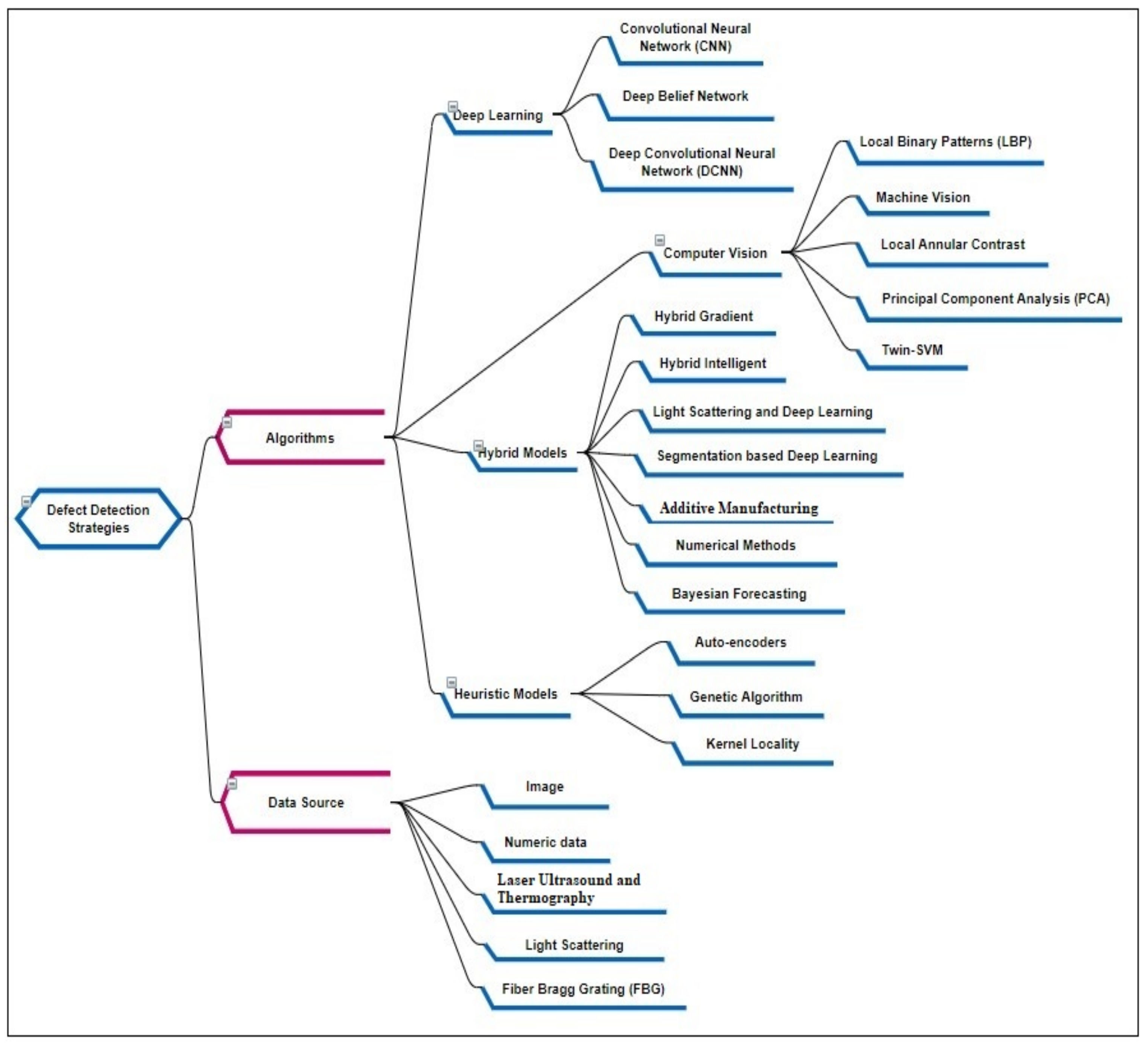
AI landing has made significant progress and is in high demand for quality control in product-based industries. Even though the traditional techniques for defect detection using geometric filters have been utilized, their accuracy and ability to identify new categories of defects are lacking. Therefore, we have designed an ALDB-DL system that can provide defect detection for multiple defect categories by using computer vision and deep learning algorithms to gain higher accuracy during process automation. The literature survey presents different defect detection algorithms as summarized in Figure 1, which include algorithms for computer vision, deep learning, hybrid methods, and heuristics. Data sources also indicate various types of datasets collected from different sources used in the feature learning of hybrid algorithms.
The deep learning-based models used in defect detection in the industrial environment include CNN, Deep Belief Networks (DBNs), and Deep Convolutional Neural Networks (DCNNs).
A laser-powder bed fusion-based deep learning model using monitoring by in-situ thermographic was presented by H. Baumgarti et al. [11]. A new technique of melt pool monitoring for printing defect detection was proposed, which uses a thermographic off-axis imaging data source and a deep neural network. The delamination and splatter defects were recognized with high accuracy using class activation-based heatmaps. A new object detection framework for hot-rolled steel defect detection using a classification priority network was demonstrated by D. He et al. [12]. The multi-group CNN (MG-CNN) was used for classification, and then feature maps for different defects were extracted by using different convolutional kernels independently. Later, the end product-based corrosion and wear resistance defects were evaluated with good accuracy. A lithium-ion battery inspection method for defects using a convolutional neural network was presented by O. Badmos et al. [13]. The microstructural defects were detected by using sectioned cell light microscopy images and CNN. The pre-trained networks showed better classification accuracy utilized in quality control. Metallic surface-based automatic defect detection and identification with CNN was demonstrated by X. Tao et al. [14]. A cascaded auto-encoder (CASAE) was used for images from the industrial environment for obvious defect contours with contrast, and less noise within the illumination condition helped with defect segmenting and localizing. Selective laser melting (SLM) defect detection by acoustic signals applying deep belief networks was presented by D. Ye et al. [15]. A simplified classification structure was applied in SLM for 3D metal printing by using deep belief networks and recording acoustic signals for porosity, surface roughness, crack, and delamination defects detection. Casting defects detection using a deep convolutional neural network (DCNN) was demonstrated by J. Lin et al. [16]. A new vision mechanism and feature map by deep learning was proposed, which used intra-frame attention strategy and inter-frame DCNN for overcoming false detection and missed detection, respectively, with high accuracy. A track fastener defect detection method for railways using image processing and deep learning was presented by X. Wei et al. [17]. A dense-SIFT novel fastener defect detection and trained VGG-16 for recognition were utilized for automation and improving track safety. Later, faster region-based convolutional neural networks (R-CNN) were utilized for improving detection rate and efficiency. Industrial welding defect detection by overcoming various production artifacts is demonstrated by P. Tripicchio et al. [18]. DenseNet-121 deep learning architecture was used with pre-trained injector images (INJ), ImageNet, and the materials in context (MINC) dataset for detecting fuel injectors welding defects. The pre-filtering suggested usage could avoid custom-designed networks retraints. A novel model for product quality control using a convolutional neural network was presented by T. Wang et al. [19]. A deep CNN model was constructed consisting of 11 layers of convolution and pooling, which extracted defects features effectively with less prior knowledge from different background textures.
The computer vision models referred to consist of local binary patterns (LBP), machine vision, local annular contrast, principal component analysis (PCA), and twin-support vector machines (SVMs). Hot-rolled steel stripped surface defect detection using the LBP-based noise-robust method was demonstrated by K. Song et al. [20]. A modified threshold scheme of LBP used an adjacent evaluation window; thus, intra-class changes by feature variations and the changes of illumination and grayscale were used for defect detection. Weld defect detection and classification using machine vision was presented by J. Sun et al. [21]. A gaussian mixture model was used with a modified background subtraction method for defective welds feature extraction. The defect types detected included weld perforation, weld fusion, cold solder joints, and pseudo-defects. Steel bar surface defects detection by a real-time inspection algorithm using local annular contrast was demonstrated by W. Li et al. [22]. Local annular backgrounds with large contrast are used for overcoming grey fluctuating values in defect detection and are helpful for smoothing noise. The detected defect types are pits, overfills, and scratches. An in-situ magnetic resonance imaging method used for defect detection in rechargeable lithium-ion batteries was presented by A. llott et al. [23]. PCA was used to group the induced magnetic field changes in cells to check the electrode materials level of lithium incorporation and thus diagnose defects observed during assembly. A method for steel surface defect recognition based on twin-SVM and multi-type statistical features was demonstrated by M. Chu et al. [24]. Multiple statistical features were used to extract dummy boundary and representative samples, and insensitive affine transformation of scale and rotation was used with a twin-SVM for solving the multi-class classification problem.
The hybrid models studied include hybrid gradient, hybrid intelligence, light scattering, and deep learning, segmentation-based deep learning, additive manufacturing, numerical methods, and Bayesian forecasting. These models are combined with data sources that include images, numeric data, light scattering, fiber Bragg grating (FBG), laser ultrasound, and thermography. A surface defect detection method using image registration and hybrid gradient segmentation was presented by G. Cao et al. [25]. Gradient threshold segmentation was used to detect faults in the background area covering uneven illumination, and image registration with image differences was used for detecting different image shapes and appearances. A hybrid intelligent method for rail defect depth classification was demonstrated by Y. Jiang et al. [26]. The hybrid approach used a support vector machine (SVM), wavelet packet transform (WPT), and kernel principal component analysis (KPCA) for high accuracy laser ultrasonic scanning of collected defect locations and interferometer. The feature fusion helps to accurately evaluate artificial rolling contact fatigue (RCF) defect in different depths. A light scattering and deep learning method for surface defect detection on machines was presented by M. Liu et al. [27]. The deep learning model utilized light scattering pattern defects, which were predicted by a forward scattering model for any surface topography with homogeneous material. A deep learning method for segmentation-based surface defect detection was demonstrated by D. Tabernik et al. [28]. The deep segmentation network consisted of max pool and convolution layers, which were then fed to a decision network with max and average global pool layers for defect detection of plastic embedding in electrical commutators. A laser ultrasound and thermography comparison method for additive manufacturing for defect detection was presented by D. Cerniglia et al. [29]. Laser ultrasound had better flaw evaluation by A-scan signal, whereas laser thermography had robustness and was easy to establish, which was evaluated by FLIR Research IR v3.4. Numerical evaluation of thread rolling process defect detection was demonstrated by P. Kramer et al. [30]. The rolling thread process was observed by sensors measuring forming forces in radial and feed direction, where the numerical evaluation is validated by geometric and force measurements. Bayesian forecasting for high-speed train wheels’ defect detection was presented by Y. Wang et al. [31]. It presented a real-time defect detection by Bayesian dynamic linear model (DLM) supported by prognosis, potential outliers, change-detection, and quantification using FBG sensors.
Heuristic models fall into various categories, such as those with auto-encoders, genetic algorithms, and kernel locality. A multitask learning method with denoising auto-encoders for defect detection in high-speed railway (HSR) insulator surface was demonstrated by G. Kang et al. [32]. A fast R-CNN, deep material classifier, and deep denoising auto-encoder were used for localization, classification, and anomaly score calculation, respectively. A binarization method using genetic algorithm and mathematical morphology for steel strip defect detection was presented by M. Liu et al. [33]. Non-uniform illumination and defect information was enhanced by mathematical morphology, and then the genetic-based binarization method was used for evaluation. A kernel locality and curvelet transform for slab surface detection were demonstrated by Y. Al et al. [34]. A curvelet transform, Fourier transform, Fourier amplitude, and statistical features were computed, which was reduced by kernel locality preserving projections and then classified by SVM.
Therefore, the achievements of ALDB-DL could be promising for dealing with the shortcomings observed in the literature survey:
- ALDB-DL presents an architecture, hardware, and software integration-based AI landing architecture. Ultimately, a clear view of the model setup within the industrial environment is disclosed;
- The hybrid approach based model provides high accuracy by treating multiple defects independently;
- A multi-camera view for defect detection presents results exclusively on different screens/displays;
- The pseudo-code for the algorithm is given in detail and is practical to implement.
Section Plan
The present research is organized as Section 3 contains architecture, functioning, system model, the algorithm, flowcharts, and their respective descriptions. Section 4 presents the system configuration, dataset details, experiments, and results. Finally, the conclusion of the research, and the acknowledgments and references are presented.
3. Materials and Methods
3.1. ALDB-DL Initial Environment Considerations
The ALDB-DL methodology section begins with specifying the initial environment which is considered to be necessary for the implementation of the AI-based hardware and software integration:
- AI landing: AOI has proven to be a basic utility for the AI landing process in defect detection. Baseline performance has been carefully studied using feature leveraging and evaluation. For the operations, we used training data, data-based labeling, and specifications;
- For different defects, the sample area coverage, the field of view (FOV), computer vision, and deep learning-based classification needs to be integrated for high accuracy evaluation. Thus, AI landing proves to be an accurate evaluation system for the industrial defect detection environment;
- Resource specification: Implementation of AI landing in the industrial environment needs to be pre-planned by resource specifications. The ALDB-DL system includes multiple resources such as hardware setup, software integration, and resource coordination. The detail specification include programmable logic controller (PLC) module, inter-connection structure, cloud database, output results presentation, multi-camera configuration, supervisory permissions, and machine control.
- Process synchronization: Process planning with the synchronized tasks is a crucial requirement for an automation workflow. Integration of hardware, software, and AI model, once viewed as a challenge, can be effectively designed and implemented. A proper architecture model presents optimal stepwise operations for process synchronization. Henceforth, an efficient system was obtained, and quality was controlled within the industrial environment.
3.2. ALDB-DL Architecture
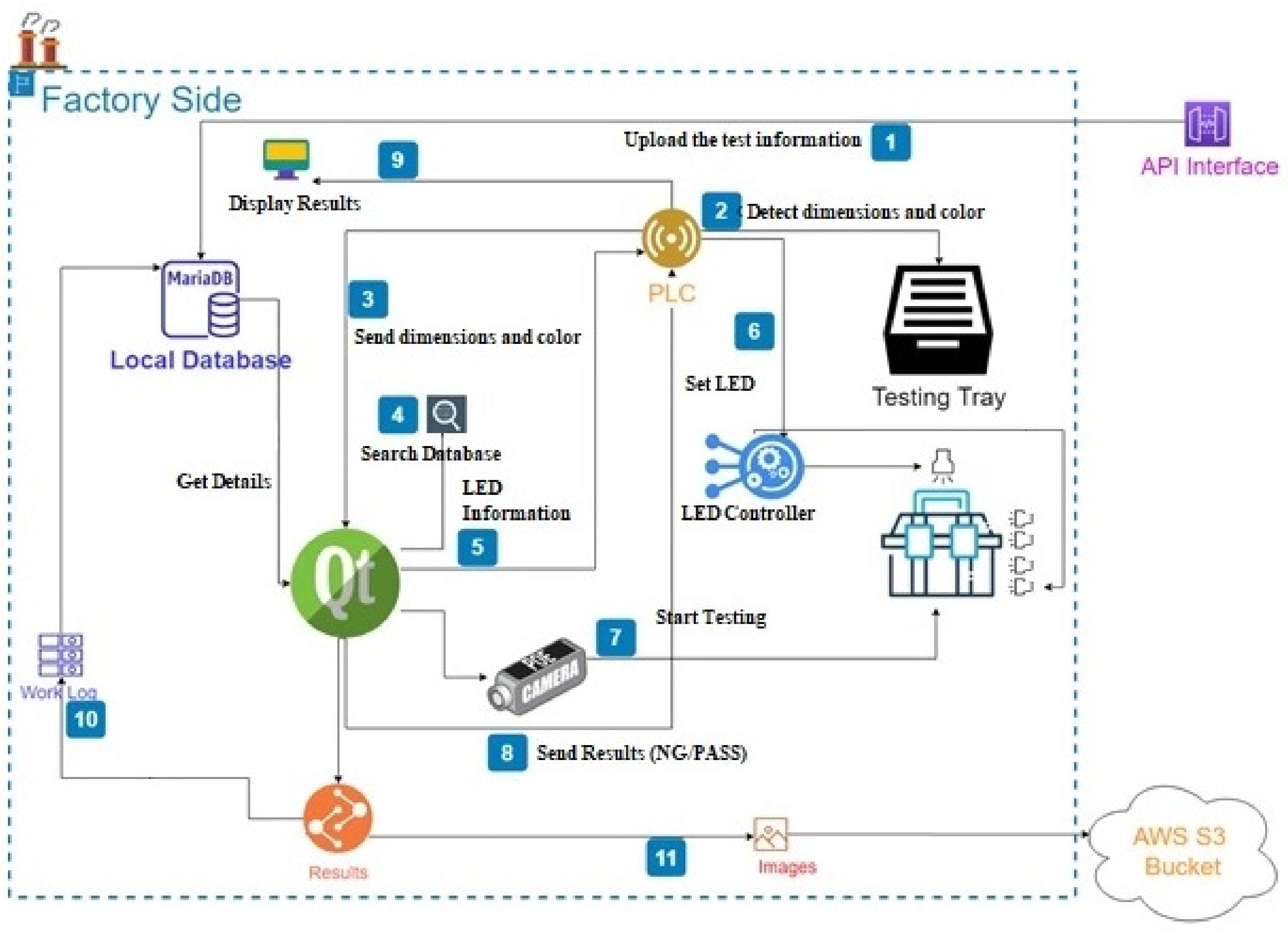
The ALDB-DL architecture designed for the industrial environment consists of various components that include PLC, LED controller for the display illumination, display terminal, local database, multi-camera setup, AWS cloud storage, and an input tray for defect evaluation. The operations within Figure 2, the ALDB-DL architecture, are detailed below:
- In step 1, the application program interface (API) executable is started to upload the test information. In step 2, the PLC as the main hardware controller checks for the input materials specification is added (dimensions and color) related to the test sample. In step 3, the PLC forwards the detailed request to the central software server as a quality terminal (Qt). In step 4, the Qt feeds the requested samples tests data to the local database for storing the details of the sample test as records. In step 5, as per the input sample size and color, the LED light values are set for the appropriate best condition illuminations.
- In step 6, the PLC sends a command to the LED controller as per the LED lights level values. In step 7, The Qt then starts the defect detection using a multi-camera model check from the Local database for the respective training for the classification and later evaluates the defects on the test samples. In step 8, the results obtained after the detection are then passed to the PLC, which in step 9 is displayed on the out screen for the detected defect type as AOI. In step 10, the data is also stored in local database as reference to the work log, whereas in step 11, the data as output results in stored in AWS S3 cloud storage as a backup for future reference and for later use of analysis of reports.
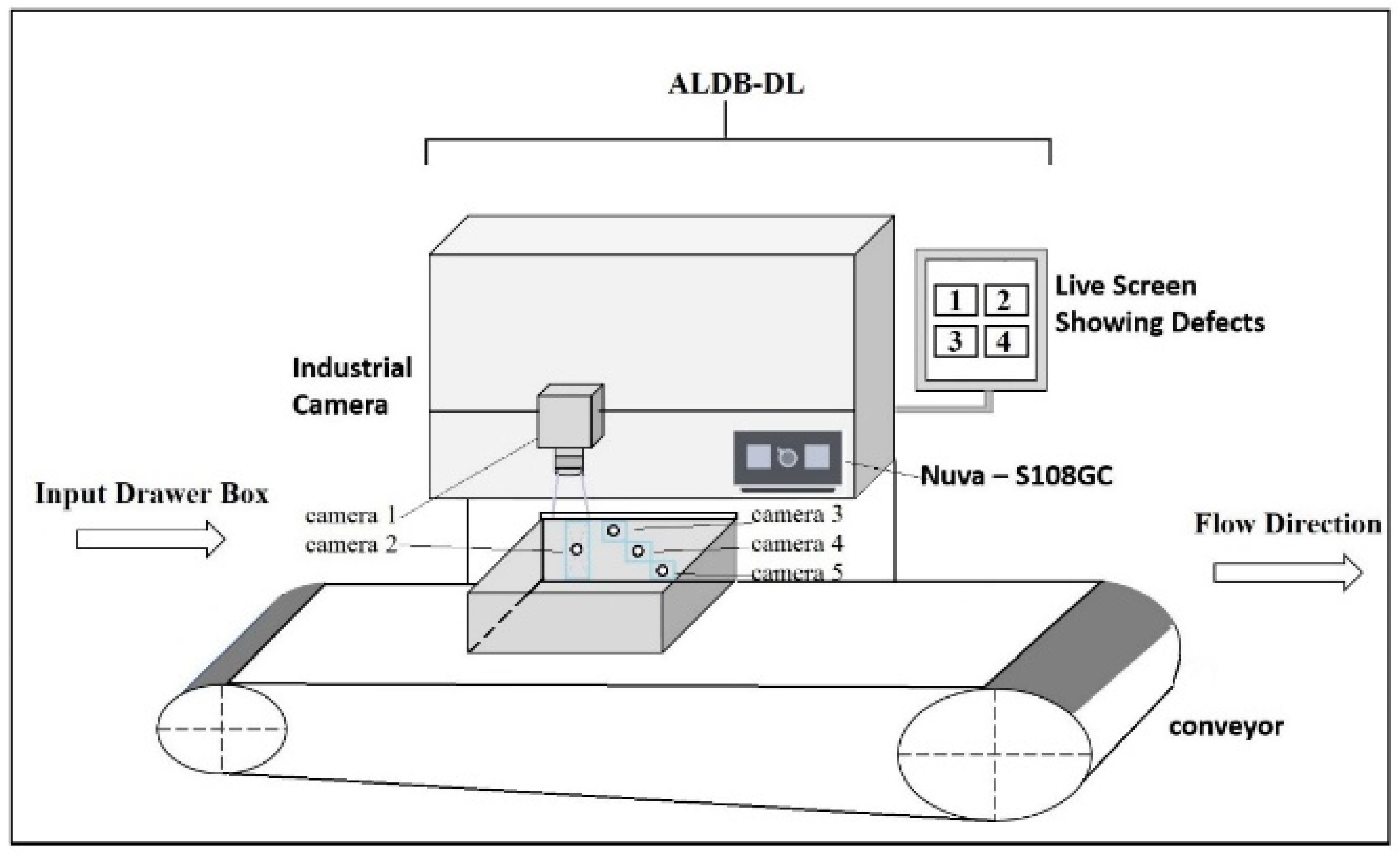
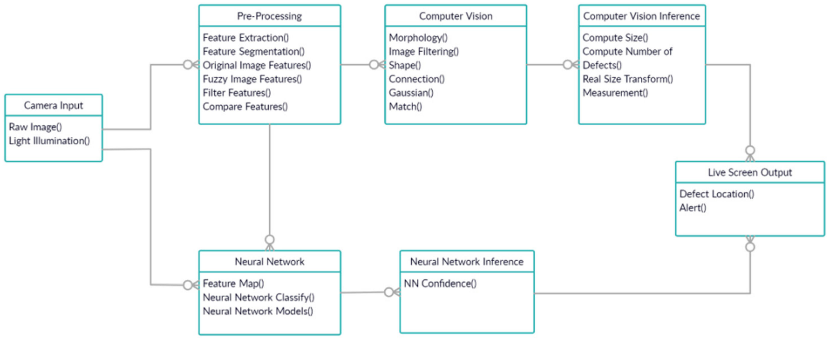
The ALDB-DL system model (Figure 3) contains four elements, the input to the system, AI landing for the manufacturing system, detection and classification using computer vision, deep learning, and live screen defect detection for industrial processes.
3.3. ALDB-DL System Model
- The input is given to the system: The input given to the system is a sheet metal-based drawer box for detecting defects on the panel and its front edge. The input configuration is required to be specified at the start, which provides optional settings for the evaluation;
- The AI landing approach: The AI landing process consists of hardware and software integration then applying AOI for the input drawer box defect detection. Initially, when the processed material in the final stage needs to be inspected for quality control purposes, it is passed via conveyer to the ALDB-DL system. The Figure 3. ALDB-DL system model shows the camera’s placed in horizontal (side) and vertical (top) direction for the panel front and edge detection respectively. The defect detection on the edge will be performed by a deep learning algorithm based vertical (top view) camera. Whereas for the front panel, both computer vision and deep learning is implemented. A Nuva-8108 GC industrial camera are used for the images captured for best focal;
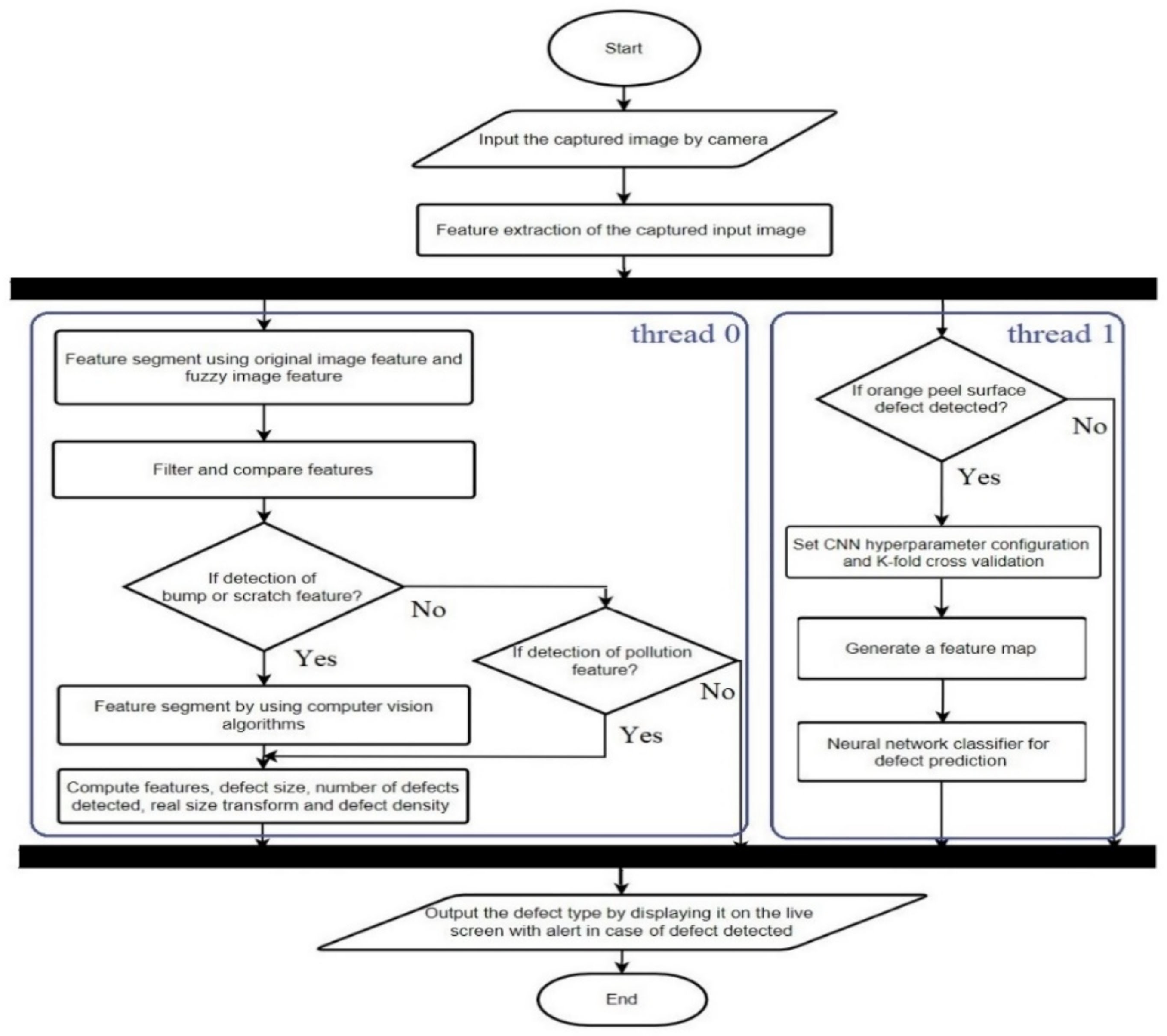
- Detection and classification using computer vision and deep learning: The defects are first detected on the drawer box front edge and panel, which is then classified by using either computer vision or deep learning algorithm. The ALDB-DL system model (Figure 3), indicates the inclusion of the cameras, where camera 1 shows the top view, and cameras 2 to 5 show the front panel view. Cameras 1 and 2 are used to detect orange peel defects, and deep learning is used here for better accuracy. In the case of cameras 3 to 5, they are used to detect scratches, bumps, and pollution/dust defects, where computer vision works accurately. Therefore, at the start, the input image is taken by each camera, whose features are then extracted. Figure 4 and Figure 5 shows in detail functioning. To implement computer vision and deep learning on live screen in parallel, two separate threads are used, one for computer vision and two for deep learning. Therefore, thread 0 executes the computer vision algorithm; feature segmentation is performed by computing for the original image and fuzzy image features, which are then filtered and compared to capture the details. When a bump or scratch is detected, then feature segmentation by computer vision is performed that includes image fragment connection, image filtering for enhancement, gaussian for image smoothing, matching for similarity measurement, feature space, search space, and search strategy computation. Image morphology for the non-linear operations is performed by collecting the image shape. The shape feature is used for identifiability and invariance of rotation, translation, and scaling. Later, feature computing is used to obtain all the present features within the image. In the case of pollution defects, only feature computing instead of feature segmentation by computer vision is needed as they are not complex to detect. If no defect is detected after feature segmentation other than bumps, scratches, or pollution, then the image is considered to be defect-free, and the thread is completed at the end. Once the defect features are computed, then the size of the defect and the frequency of every defect are calculated based on the specification of the defect size threshold as estimated by the supervisor. For the result details, the detected defect size and density are calculated. Ultimately, the defects are displayed on the live screen with the red highlighting, and the alert is raised when defects are detected by the ALDB-DL.
For thread 1, deep learning models of Inception, MobileNet or LeNet are used for the detection of orange peel. Initially, the CNN hyper-parameter configuration is set, and k-fold cross-validation is performed. In the successive steps, a feature map of the input image is generated, which is later on, classified by the NN classifier for defect prediction. Once the respective defects are detected, then the defects are displayed on the live screen with an alert.
- Live screen for defect display: The real-time defects on the sheet metal-based drawer box can be detected while it is passing over the conveyor. The ALDB-DL system helps to perform the quality inspection by identifying drawer box defects, which are then highlighted and displayed on the live screen with respect to the defect type. Therefore, the defect raises an alert that notifies the machine operator at the quality control checkpoint. A live screen display of real-time defects is convenient for the industrial process automation system.
3.4. Algorithms
In this section, a detailed description of the algorithms is presented that will explain the two-stage model of ALDB-DL. The algorithms included here consist of an AI landing algorithm for defect detection, AOI for computer vision, and AOI for deep learning. The discussion for software architecture is detailed in Section 5.2.
Algorithm 1 for AI landing drawer box defect detection is presented in the form of pseudo-code. In step 1, the input image is taken by the algorithm from the industrial camera for processing. In step 2, candidateSet 1 is taken as input after processing by the computer vision algorithm. In steps 3 and 4, candidateSet 2 and candidateSet 3 are taken as input after processing by neural network algorithm. In step 5, the output given by the AI landing algorithm is candidateFinal, which is the hybrid output based on multiple algorithms. In step 6 the candidateFinal is initialized to null (∅). In step 7, from the current input image (Imagei) the features are extracted based on the pre-processing steps, including feature segmentation, original image features, fuzzy image features, filter and compare features for every image fragment based on the respective color as the naïve segmentation algorithms are not effective. In step 8, the fuzzy image features can be extracted after converting them to gray scale. In step 9, the discrimination of fuzzy image is performed to obtain the membership object having a better classification of the object and background. In step 10, Shannon’s entropy function is applied to the membership object (MembershipObject) to obtain fuzzy divergence (DivergenceFuzzy) for checking disorder and variance within the image context. In step 11, filtering is performed by a supervisory specified threshold within the image features, and fuzzy divergence for obtaining segmentation features (SegmentationFeature) utilized later for computer vision with the supervisory defect specification rules as given in Appendix A, Table A1. In step 12, the If condition checks whether the segmentation feature contains bump/scratch/pollution defect types. If yes, then in step 13, an independent thread is created from its parent process by passing segmentation features to the AOI for computer vision algorithm, checking for which defect type is detected and is stored in candidate Set 1. In step 14, if an orange peel defect is detected in an input image feature, then a new thread is created for neural network processing, and the results are stored in candidate Set 2 of step 15. In step 16, all the detected and classified defects are added to candidateFinal, if present, and, in step 17, is returned by the algorithm.
| Algorithm 1 AI Landing Algorithm for Drawer Box Defect Detection. |
|
Algorithm 2 contains the pseudo-code for the AOI-based computer vision algorithm. In step 1, the input given to the algorithm is the SegmentationFeature, which is an argument passed by Algorithm 1 after pre-processing and feature segmentation. In step 2, the output of this algorithm will be candidate Set, which identifies defects by using computer vision. In step 3, the candidate Set is initialized to null (∅). In step 4, if feature segmentation is equal to a bump feature or scratch feature, then a code block containing feature computing is executed otherwise, for pollution features, no feature computing is required, as it is recognizable with ease. In steps 5 to 8, the operations performed using segmentation features include MorphologyBinary_Opening (fm), filtering (ff) of shape (fs), and connection (fc) for non-linear operations, enhancement, identifiability, and invariance of image registration, respectively. In step 9, map features combine all the operated operations (fm, ff, fs, and fc), and results are unified. In step 10, the previously mapped features are then given as input to the gaussian and shape function by first removing the noise then separating bump and scratch defects, respectively, which in step 11 are stored as DefectFeatures. In step 12, the defect size and density are computed from the defect features to be stored as candidate Set. Finally, in step 13, the candidate Set is returned by this algorithm to the calling function.
| Algorithm 2 AOI for Computer Vision Algorithm |
|
In Algorithm 3, the pseudo-code for AOI based neural network algorithm is presented. In step 1, the image features(ImageFeatures) are taken as input by this algorithm. In step 2, the output generated by this algorithm is the candidate Set, which contains the neural network-based defect classification. In step 3, the NNConf is used to present the defect type prediction by the neural network model as orange peel. At step 4, the candidate Set is initialized to null (∅). In step 5, the feature map of the image features is generated to be stored as the NN feature set. In step 6, the convolutional neural network with the feature set is used to obtain defect classification (ClassifyDefects) and NN confidence (NNConf), which in step 7 is stored as the candidate set. Finally, in step 8, the candidate set is returned by the algorithm.
| Algorithm 3 AOI for Neural Network Algorithm |
|
3.5. Mathematical Model
The CNN algorithm uses LeNet with (1 × 1) convolution and GAP. The GAP overcomes the overfitting issues of the fully connected layer and is easier to interpret, as the classification layer utilizes GAP over feature maps [35]. The traditional CNN uses convolutional layers and spatial pooling layers, which are alternatively stacked. It includes linear convolutional filters generated feature maps and non-linear activation function, where the linear rectifier calculates the feature maps as Equation (1):
where (i, j) is the feature map’s pixel index, weights W, the location (i, j) for the centered input patch as , and the feature map channels are the index, k.
In the case of latent concepts distribution absence, a universal functional approximation is preferred for the local patches feature extraction for abstract representation approximation. Therefore, the use of multi-layer perceptron (MLP) indicates the priority for the structural compatibility of CNN utilizing backpropagation-based training and MLP, which performs feature re-use using a deep model. Thus, it is known as mlpconv, performing calculations as given below Equations (2a) and (2b):
where, the multi-layer perceptron layer numbers are given as n, and the MLP uses the activation function of rectified linear unit (ReLU). Equation (2) in a convolutional layer can also be presented as parametric pooling of cascaded cross channel. The input feature maps by the weighted linear recombination are performed from the pooling layer, which is then processed through the rectified linear unit. The cross channel repetitive pooling is done in the successive layers as the pooled feature maps in the cross channel. Thus the learnable and complex interactions are obtained from the cross channel information.
In the case of the MobileNet network, a minimal hardware configuration can work efficiently for deep learning algorithms in real-time. The accuracy is achieved without compromise by the reduced parameters [36]. So the MobileNet classification accuracy achieved by 1/33 parameters of the standard CNN algorithms is the same. The MobileNet model consists of a separable and deep convolutional structure, which consists of depth-wise layers (3 × 3) kernels and point-wise layers (1 × 1) kernels that operates by using batch normalization and ReLU6. Therefore, the ReLU6 activation function is given as Equation (3):
where the feature map consists of the pixel value is given as z.
The MobileNet attains the reduced calculations and increases the speed of training by using the separable and deep convolutional structure. It can be given as Equation (4):
where the input and output channels are M and N, respectively, and the filter is with a feature map, G. The zero-padding fill style is used by as the input image, feature image, and feature maps for the standard convolution. × and M are the size and input image channels, respectively, and it is mandatory to N filters with M channels and the N feature image with × as the size before the output, which can be combined to present the computing cost. The formula for can be given as Equation (5):
where the filter is represented as . In the case of step size being equal to 1, after the separable convolutional structure and deep, there is invariability in the characteristics graph size by the filling of zeros. If the step size is equal to 2, the feature graph size is reduced to half by the dimensionality reduction operation after filling with zeroes.
4. Results
This section consists of all the experiments carried out for the ALDB-DL implementation, comparisons, and results. The system configuration used for the implementation and testing for the ALDB-DL is presented in Table 2. system configuration with Table 3. Industrial camera configuration. The discussion on industrial hardware configuration is detailed in Section 5.1.
4.1. The Details of the Dataset
In Table 4, the dataset provides the complete image details obtained from the industrial environment. Table 5 gives a limited dataset acquired from Ming-Chuan Industrial Co., Ltd. for defect category, and independent defect frames provide the count of defects present within the available industrial dataset, as the same defect could occur in multiple frames.
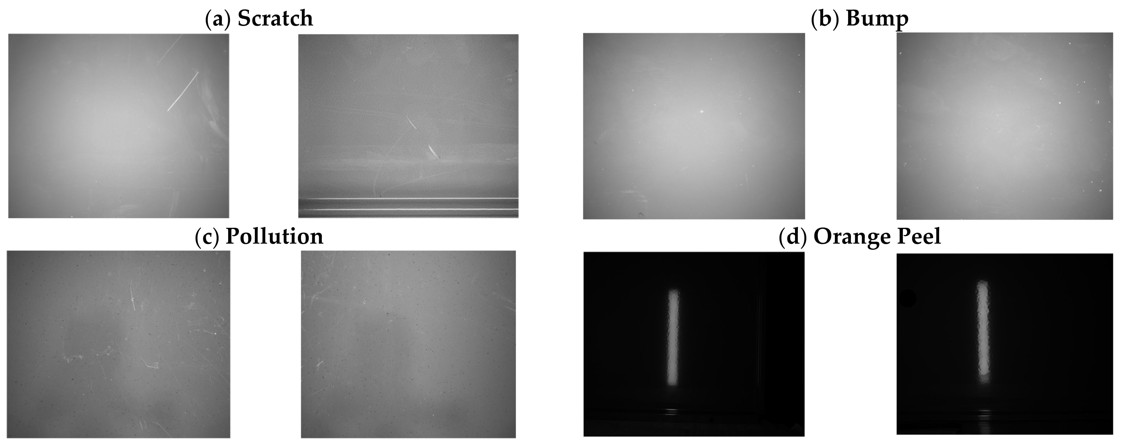
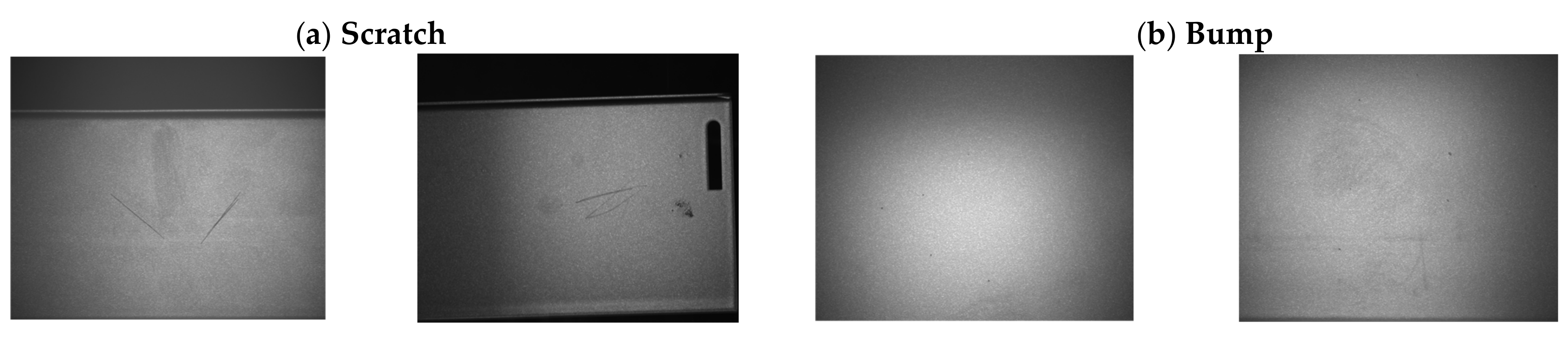
The images captured from the camera and processed by the ALDB-DL algorithms were 10 frames/sec. This dataset was used for the experiments of computer vision (scratch, bump, and pollution) from a total of 91 drawer objects of which 46 were passed and 45 did not pass (not good (NG)). The total images in computer vision were 1087, where 947 were good, and 140 were NG. In the case of the deep learning CNN model (for orange peel defects), which had a total of 1075 frames consisting of 712 passed and 363 NG. For the deep feature extraction, the configuration threshold set for training and testing was 80:20 ratios. The computer vision and CNN algorithms used for the ALDB-DL experiments constituted multiple statistical, spectral, machine, and deep learning models with various hyper-parameters for achieving higher accuracy and the best performance in the test dataset. The training data included single or multiple defects present within the single image, as the occurrence of such defects is at random. The configured CNN was then applied to the test dataset to inspect the accuracy achieved by the different CNN models. The dataset acquired for the training and testing was made available by Ming-Chuan Industrial Co. Ltd., Taiwan. Capturing the high-quality images from the industrial samples required a high definition camera that was suitable for preparing a dataset consisting of multiple different categories of defect sample images for the computer vision filtering and classification by the CNN algorithms. Figure 6 presents the different category types of defect samples of red color product images observed during an inspection by the AOI system in the ALDB-DL. Similarly, Figure 7 shows some samples for the defect sample category with black color products, respectively.
4.2. Experiment Evaluations
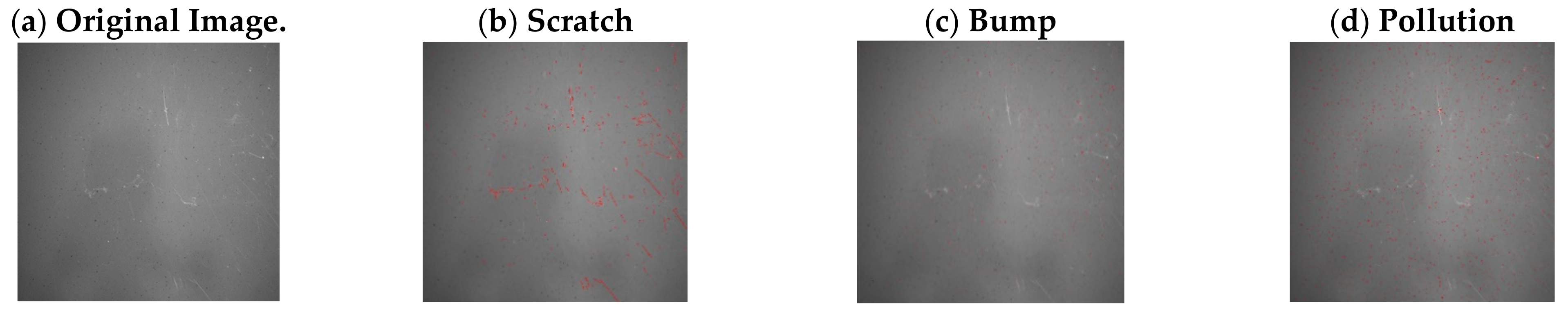
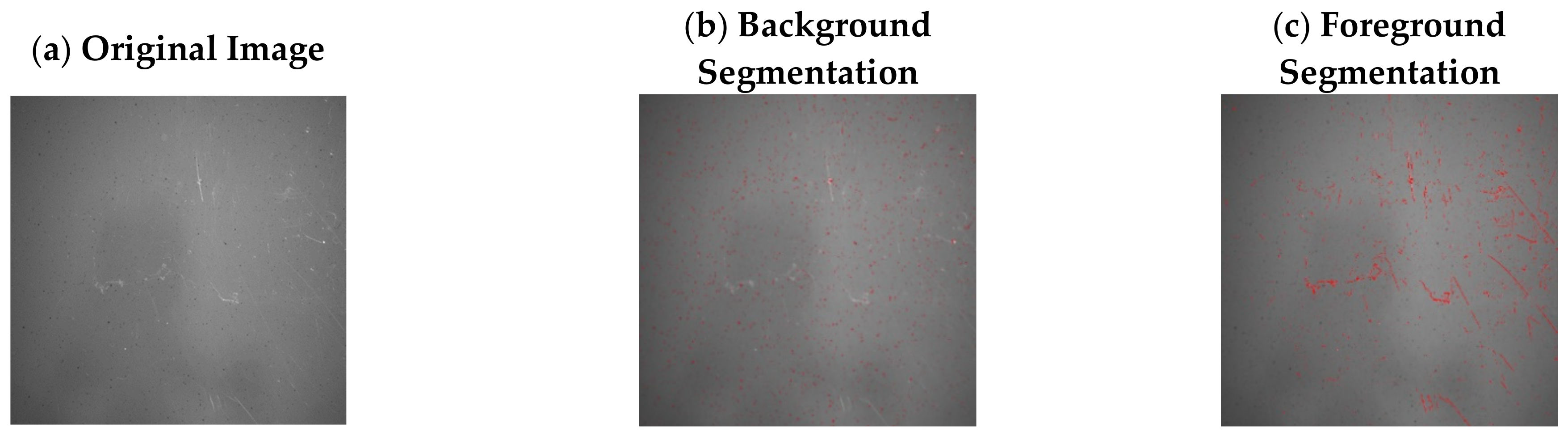
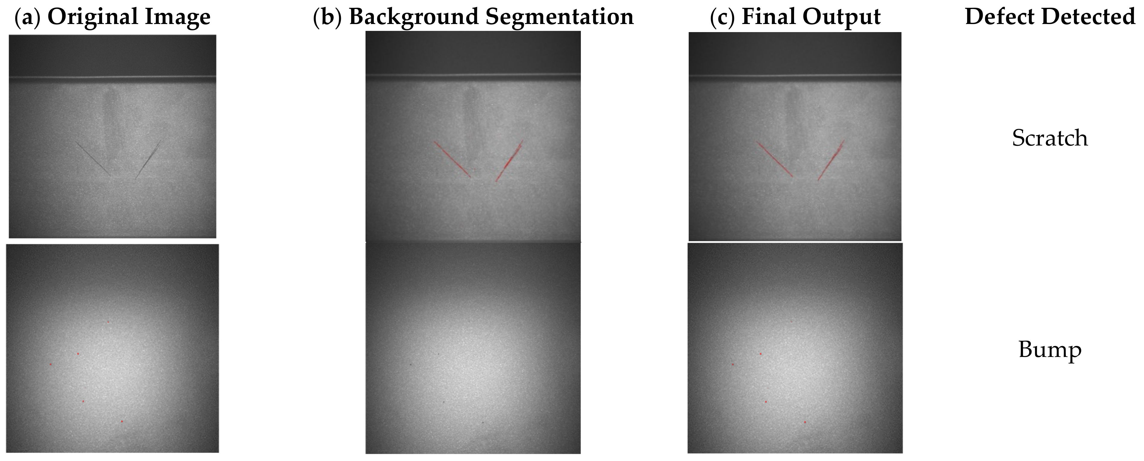
The computer vision algorithm, as stated in Algorithm 1, AI landing algorithm details the feature extraction from the image, including the color of the product. The drawer boxes were colored in either red or black, and hence the process was performed carefully while the results are presented separately to identify the peculiarity. In Figure 8, the red color product defect detection by computer vision is presented by a red color mark and is accurate to highlight it. Similarly, in Figure 9, the black color product defects were detected by computer vision and performed consistently, highlighting well even in different color products with foreground and background segmentation. Figure 10 shows the computer vision-based pre-processing on the original undefined image to get feature segmentation then used output images for determining the defect type.
Table 6 CNN functional parameters are presented, and the parameter configuration was used to set the CNN models in ALDB-DL. The height, width, and depth (color channel) are denoted by the input shape for the image measure, where the last value was for black and white images. The batch size indicates the data added in the network of blocks/batches having the size 10. The dataset passed in the form of batch size in the forward and backward direction of the neural network in a single epoch was achieved by using successive iterations. The activation function used here was softmax, also known as the normalized exponential function, and is a generalization used as multinomial logistic regression. It functions as the normalizer for the output of the neural network with a probability distribution over predicted class output in the last layer. The Adam optimizer was derived from adaptive moment estimation and was used to update training data’s network weights iteratively. It was quite beneficial for non-convex optimization problems and was quite efficient in performance. The categorical cross-entropy loss, also known as softmax loss, was used to output a probability to train CNN over the C class for each image. Basically, it was used specifically for the cases of the multi-class classification. Later, the experiments were validated by distributing them into images by train and test ratio. As shown in Figure 11, the SHAP values [35] are presented for the orange peel defect based on the dataset presented in Table 4. Defect and frames were counted to identify the feature in comparison to the prediction. The LeNet + (1 × 1) convolution + GAP layers’ configuration was a hybrid model, which used a model parameter construction based on a concept similar to network in networks (NIN) [36].
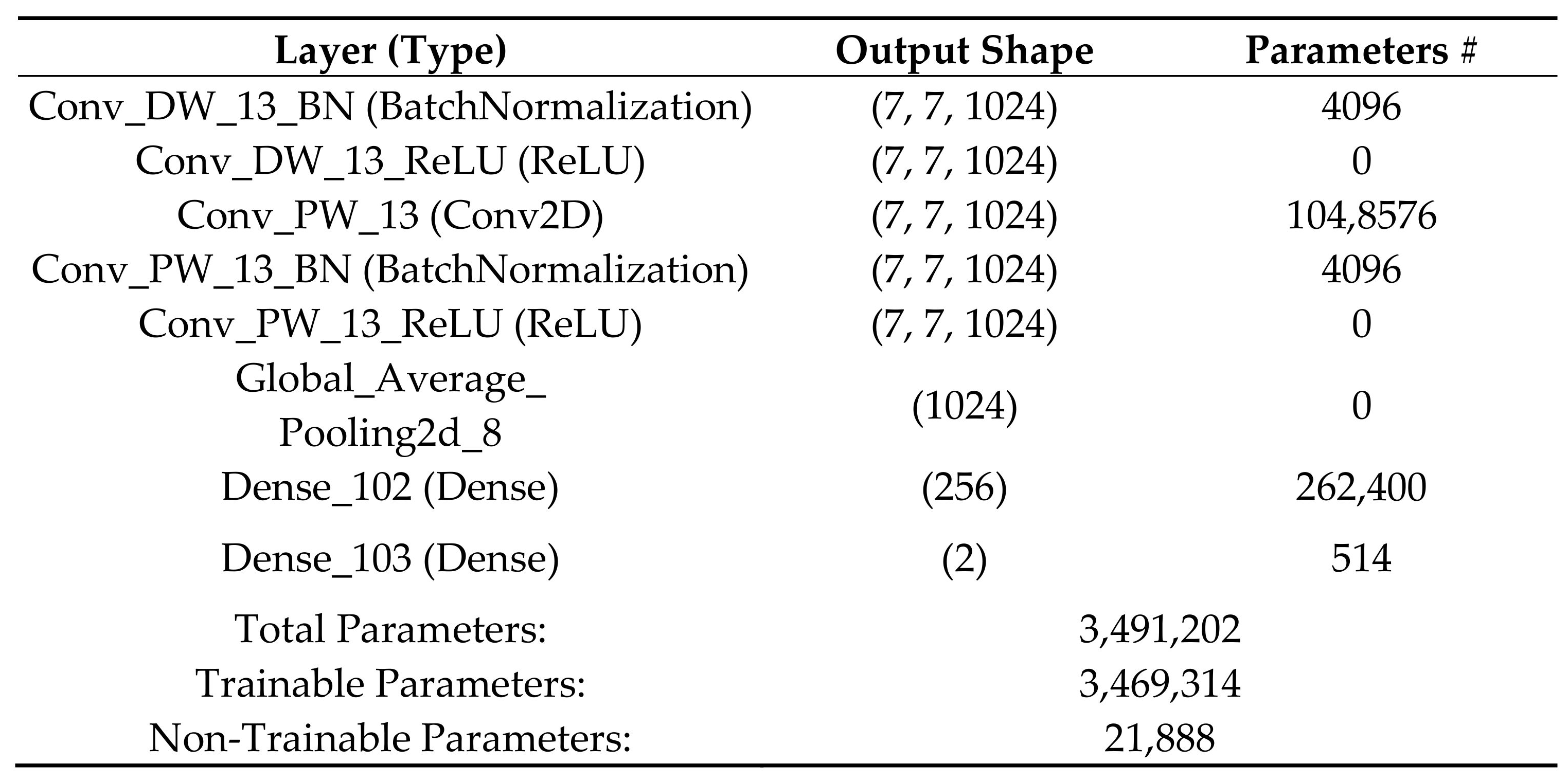
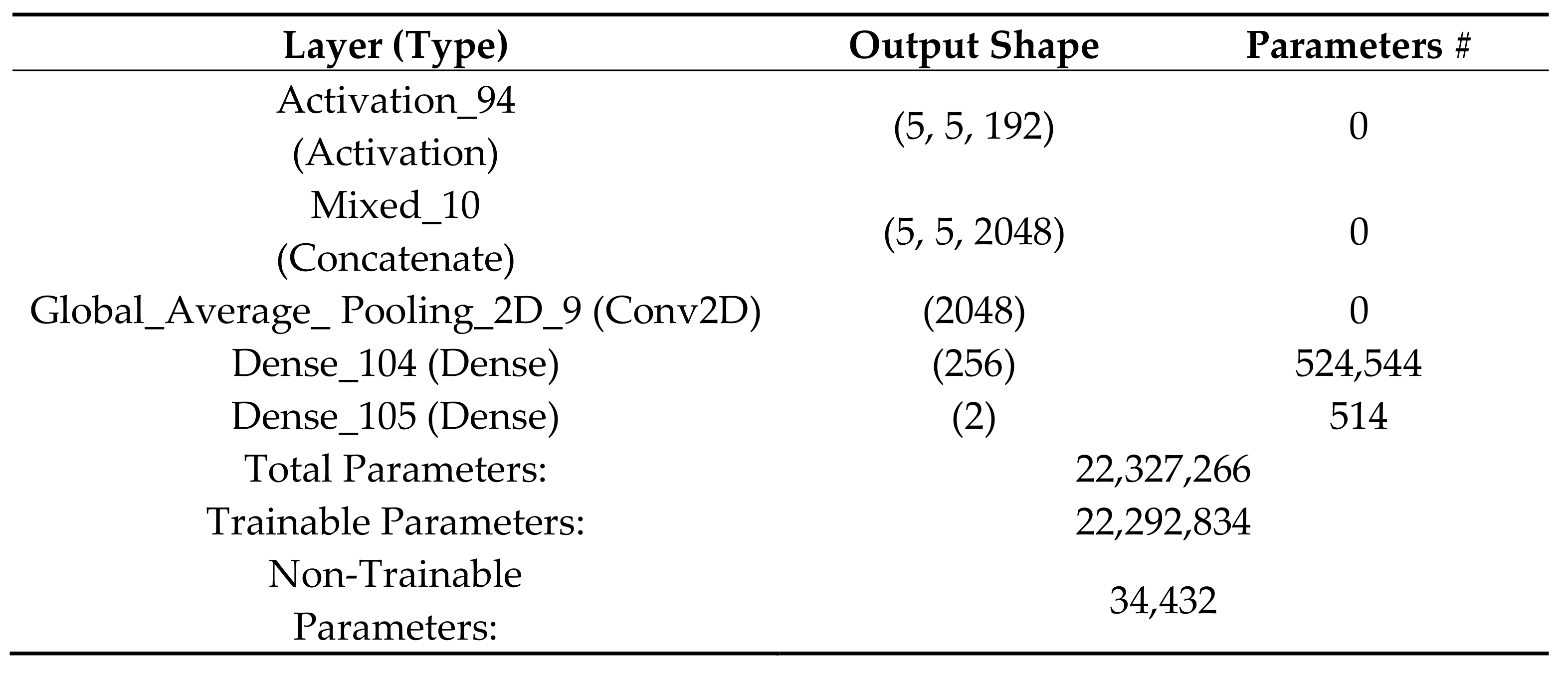
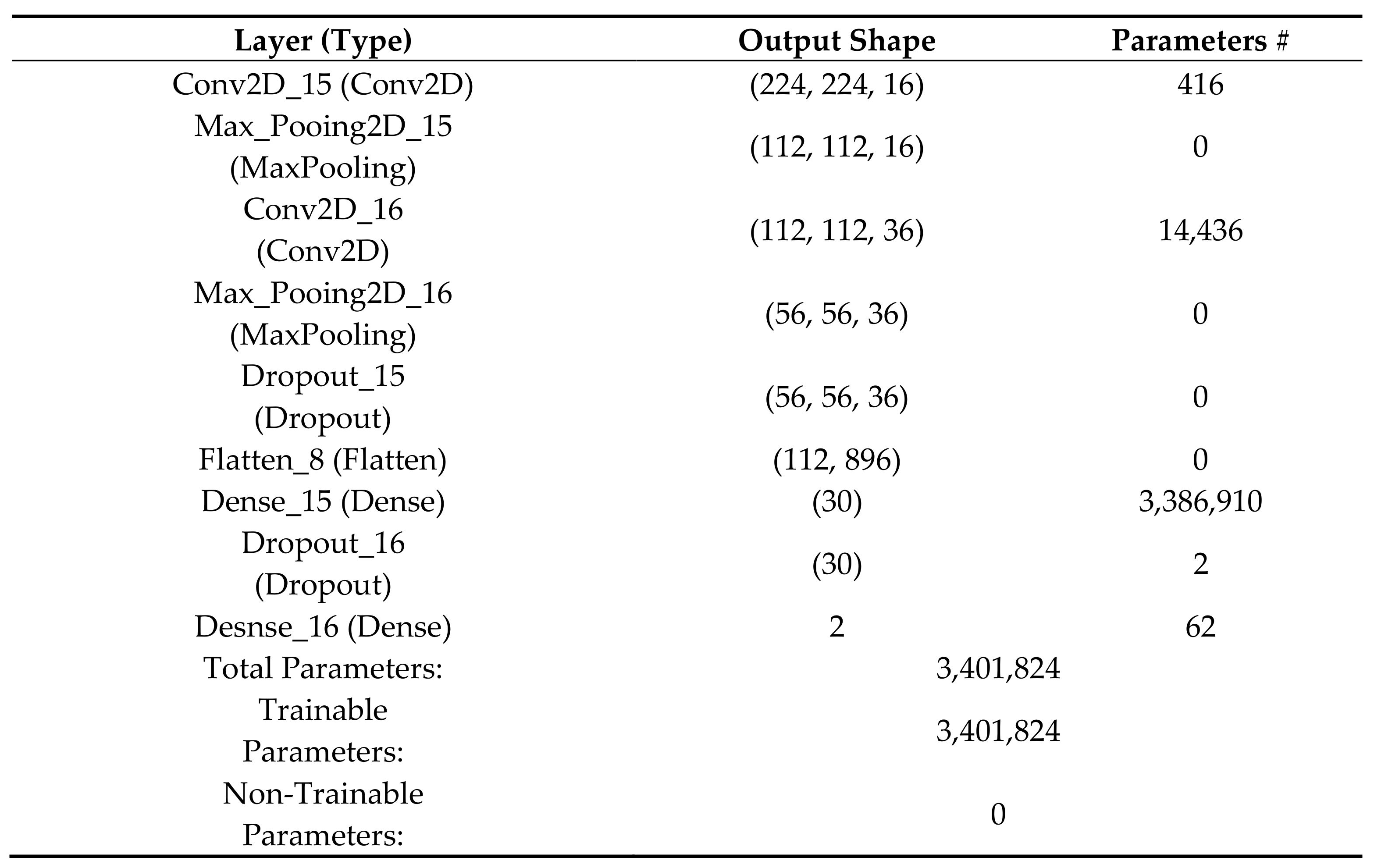
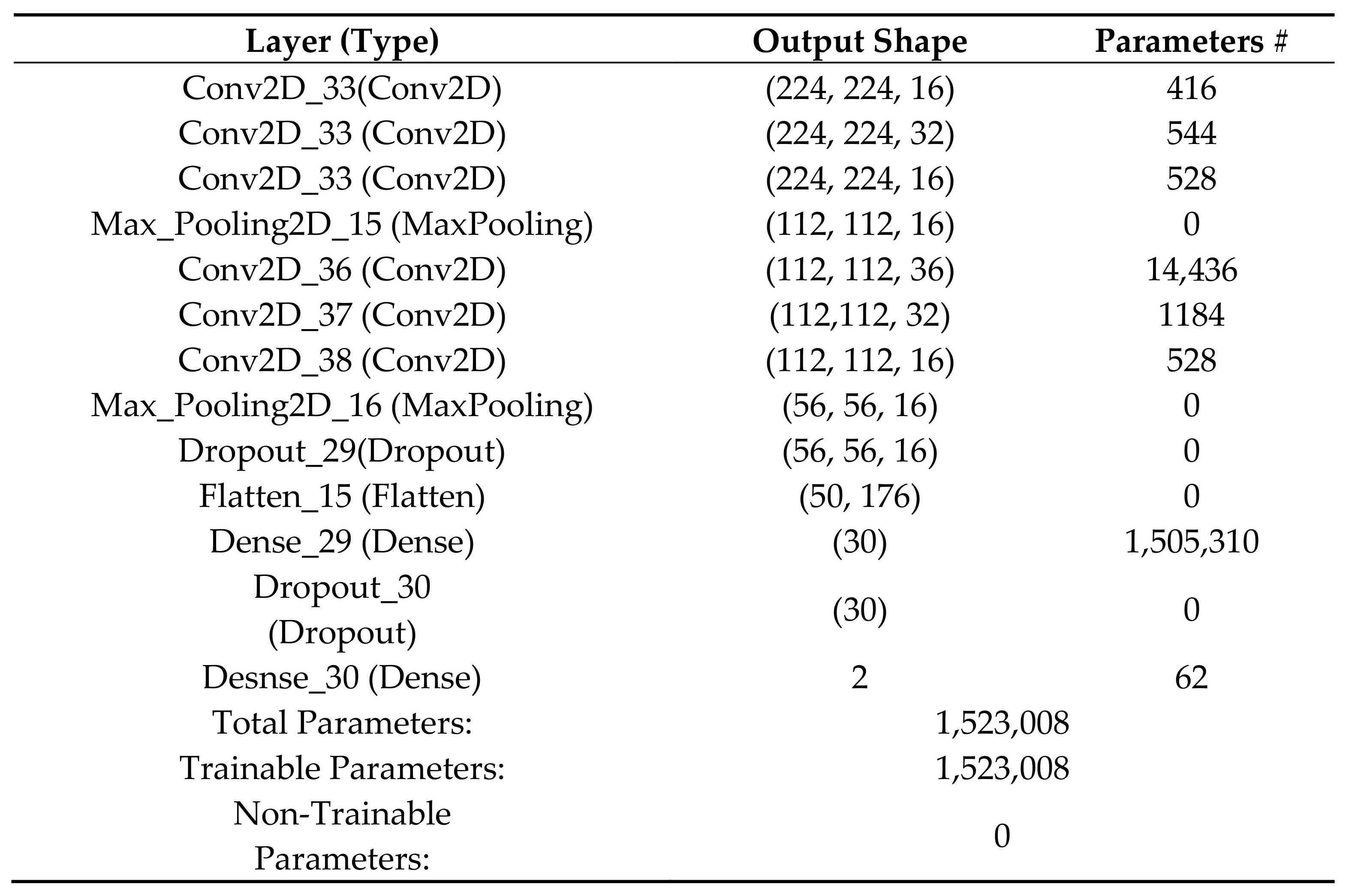
The new hybrid configured model of LeNet [37] + (1 × 1) convolution with GAP, as seen in Table 7, was found to be more efficient for the application-wise requirements for the ALDB-DL CNN algorithm. The three different models were compared here using GAP to reduce the number of dense parameters generated by each model and thus reducing the execution overhead. The use of GAP helped to reduce overfitting faced by the fully connected layers as well as improves the generalization ability. The detail layer configuration used and the results achieved by the confusion matrix are presented in the Appendix A section in the form of Figure A1, Figure A2, Figure A3, Figure A4 and Table A2, Table A3, Table A4, Table A5, Table A6. Dropout did help to overcome the overfitting issues up to some extent. Therefore, the GAP replaced the conventional fully connected layers of CNN. It was implemented by generating a classification category-wise feature map in the mlpconv layer, thus eliminating the fully connected layers by averaging the feature map as the input to the softmax layer. Henceforth they were known as category confidence maps. Overfitting was avoided by optimizing parameters of GAP, and GAP was found to be robust by summing the spatial information for the input’s spatial translation. Ultimately, the GAP was recognized as a structural regularizer by utilizing feature maps as the concept’s confidence map, which was obtained by using mlpconv layers. From Table 6, it can be seen that the most optimized parameters were achieved by LeNet + (1 × 1) convolution with GAP, and the accuracy results were the best in comparison with high parameter generation leading to an improvement over other popular CNN algorithms.
where (true positives) was used to indicate if the defect was detected specifically as not good (NG) and the model had predicted it correctly. True negative for the outcome as good. False positives (FP) indicate the CNN model predicted the outcome as good, whereas the actual value was NG. False negatives (FN) indicate predicted outcome was NG while the actual outcome was good.
Accuracy depends on their values present within the respective matrix, which is shown in Equation (9):
The classifier evaluation was accurate based on the evaluation by the calculation of true positives combined with true negative () divided by total values. In Table 7, the various CNN algorithms, each with k-fold cross-validation, are compared based on confusion matrix results having precision as actual accuracy for positive results prediction in equation, recall for the actual positive output as how much could be recalled, F1 score as the measure of a test’s accuracy and the complete model’s accuracy based on both positive and negative values, which are given by Equation (6) to (9) respectively. The computation time is presented as 1 frame and 10 frames per second processing for all of the CNN algorithms to compare and inspect for the best performance. As the accuracy and computation times of different CNN algorithms were found to be quite similar and hard to differentiate, therefore the dense parameters configuration is shown, which helps to differentiate between the different dense layer parameters used within their respective CNN algorithms. Thus fewer parameters indicated minimal use of CNN configuration for the optimal performance tuning. The (1 × 1) convolution’s concept is like a fully connected layer without using a lot of parameters, which makes the network increase non-linearity to fitting in testing data. For each feature map, the (1 × 1) convolution filter considers all of them and learns their weights to choose which one was important to classify the target (defect).
Another reason we used (1 × 1) convolution is it could perform dimensionality reduction; if the parameter was lower, then the prediction speed would be faster. As using the (1 × 1) convolution filter after the convolution layer and the (1 × 1) convolution filter was smaller than the convolution layer, the output shape changed because of the filter numbers when comparing the max-pooling layer output shape, so after flattening, the total parameters were half of the previous model.
The GAP could be applied to the Inception and MobileNet CNN by replacing the flatten layer with it. The GAP could be re-trained by simply training it again, whereas fine-tuning could be done by freezing another layer’s weight and then training GAP. At first, we needed to change their output layer to our target because the Keras API [38] is designed to classify 1000 different objects; we changed it to classify two objects. Second, we called the GAP layer to add it before the output layer. The default model’s output structure in Keras is GAP, but we needed to change it to our target; otherwise, we could not perform training. Therefore, if we wanted to re-train the model with GAP, the most important thing was to check if GAP needed to replace the flatten layer. If we wanted to fine-tune the weight on GAP, then we needed to freeze the input and the hidden layer’s weight. Later, replacing the flatten layer to GAP (if the original model did not have a flatten layer, then only add GAP), then train it.
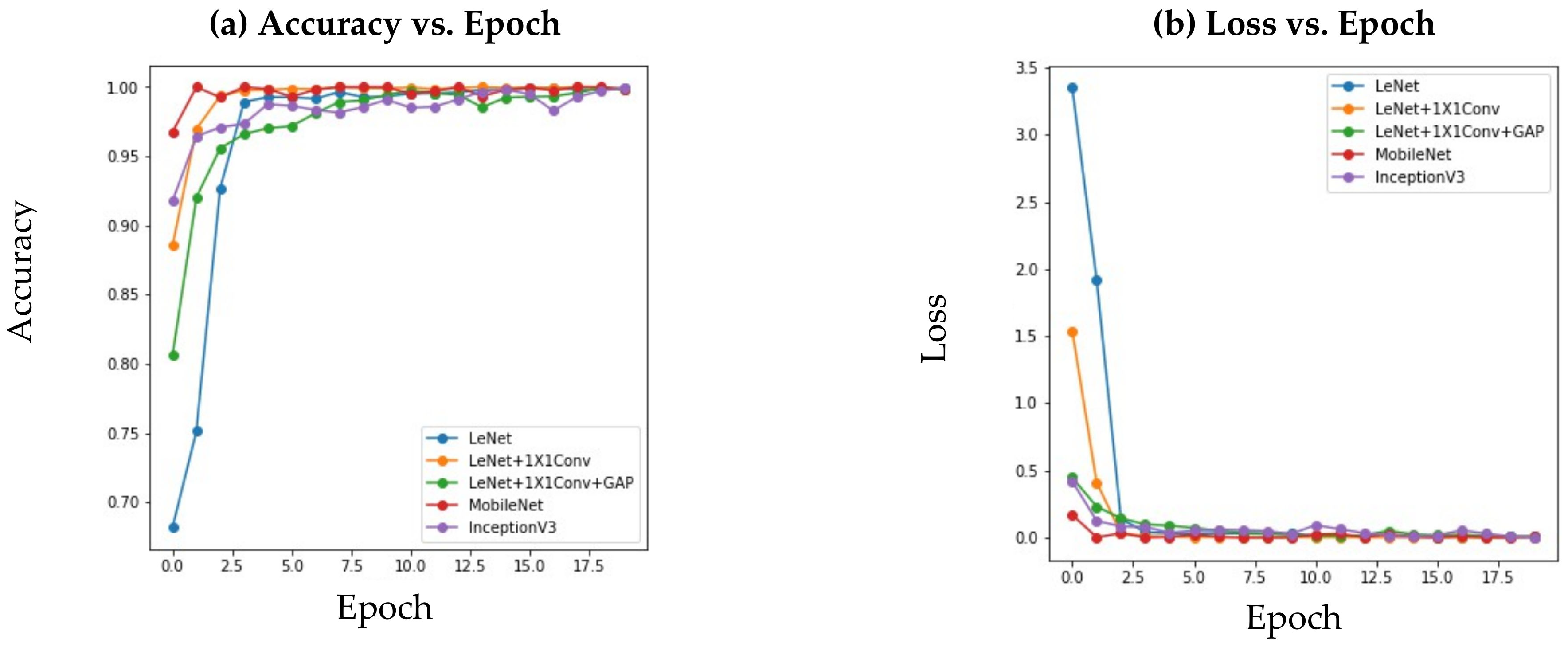
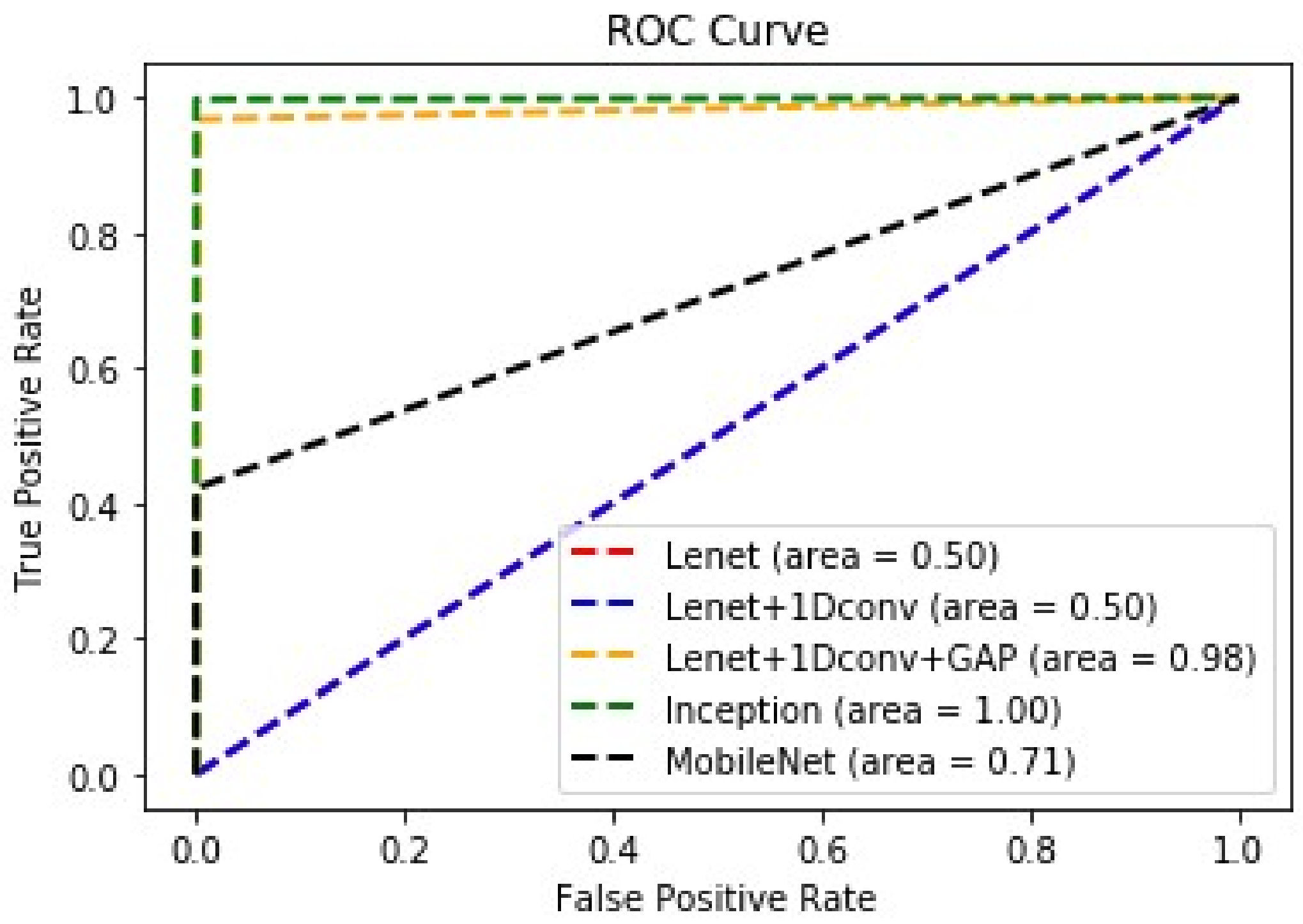
Figure 12 shows the (a) accuracy vs. epoch and (b) loss vs. epoch for the CNN algorithms. Here, the LeNet + (1 × 1) convolution with the GAP CNN algorithm was found to perform better in terms of accuracy. Whereas Figure 12b shows the loss of all the CNN algorithms was found to be similar in the epoch comparison. The ROC curve presents the diagnostic capability of the deep learning algorithms for the orange peel defect (Figure 13), where a score of 0.98 was achieved by the configured LeNet + (1 × 1) convolution with GAP.
5. Discussion
- The discussion section is crucial for understanding the AI landing process. In this section, we will give details for the basic requirements of designing ALDB-DL hardware and the technology for setting up an industrial working model:
5.1. Hardware Configuration
- Selecting an input image: The input provided to the ALDB-DL system is an image; thus, it should be properly selected by focus from the aligned cameras. The cameras should be placed in a distinct place to capture the full view of the sheet metal drawer box in parts by avoiding an overlap;
- Conveyer frequency: The industrial process includes defect detection on large quantities of finished material. In the final stage, the drawer boxes are continuously passed on the conveyer through the ALDB-DL system, as shown in the system model (Figure 3). Therefore, the camera configuration should be set for the input of frames per second (fps) must be able to capture all the parts of the drawer box synchronized with the speed of the conveyer rotation frequency. Thus, the conveyer frequency speed can be set accordingly;
- Number of cameras: The ALDB-DL system requires multiple cameras as multiple types of defects are dealt with in the industrial process. Checking the defects on the drawer box edge and the front panel needs to have cameras in different positions. The front panel is also large in size as compared to the edge; thus, the FOV of the front panel needs to be measured for best settings such that each view is partly covered by every camera for multiple defect category detection to be displayed independently on the output screen.
- Managing the flow synchronization: Multiple factors should be considered while managing the industrial production for synchronizing the conveyer, camera position, the output screen displays, and the alert mechanism. The purpose of flow synchronization is to achieve optimal hardware setup with the best quality of process synchronization. Thus the robotic arm can be eliminated by using an alert system that can help to notice the defective item or redirect the defective item to the other direction on the multi-flow conveyer belt if needed in the complete process automated environment;
- Hardware and software integration: A proper communication system needs to be established to connect various hardware and software components. A PLC is used as an intermediator that connects the hardware part of the LED controller, camera images, database server, network, and display results on the output screen. Whereas the software part of API provides input configuration interface, control database and work log, store results on the cloud, display results on the output terminal, process the computer vision and deep learning algorithms, operate the software by the supervisor, etc. A properly defined process for the system integration ensures smooth workflow for the process automation. Henceforth, integration is a crucial part of the ALDB-DL system implementation.
5.2. Software Architecture
- Available training data and its validation: The input dataset quality and quantity are important for any computer vision (CV)/AI model. Higher image quality and well-balanced defect types can further improve performance. Several challenges are faced during the processing of datasets by CV/AI models, including pre-processing, limited accuracy, multi-defect detection, performance trade-off, etc. Therefore, a novel approach is required with the flexibility to process multiple defect types with the best suitable methods for better performance;
- Multi-defect detection using a camera: Every image available from the camera consists of multiple defects, whose accurate detection is a challenge. To resolve this issue, multi-purpose industrial cameras are used by tuning the FOV for separate parts to obtain high-quality images. Every camera can then detect multiple types of defects based on the CV/DL method. The size and density of defect detection is another challenge, which is resolved using different pre-processing and CV/DL methods. In the case of computer vision, the labeling of data first needs to be compared by using feature segments which are performed using comparing original and fuzzy images. Further, computer vision algorithms are used for segmentation, which is then compared with real size transform having supervised defect specification. Considering the different sizes and densities of defects, the labeling of data needs to be trained from previously recorded different defect types for deep learning;
- Leveraging features from computer vision and deep learning algorithms: Labelling image data for defect types can be waived by computer vision filters as a baseline. Even though the computer vision after pre-processing can capture features and detect defects, i.e., scratches, bumps, and pollution, but it is not found to be flexible enough for all types of defects, i.e., orange peel defects. Henceforth, deep learning is preferred to detect such type of complex defect types. It is observed that some defect types related to shape can be well detected with computer vision, whereas the pattern from orange peel defects can be well detected using the trained neural network-based deep learning in comparison. The leveraging of features can be done using pre-processing in computer vision and applying multiple CNN models for acquiring the higher accuracy;
- Utilizing the AOI in an industrial environment: Traditional industrial environment consists of human workers checking for defects leading to insufficient quality inspection for accuracy. The use of AOI has transformed the quality control process for complete process automation to detect, display, report, and provide defect alerts. Therefore, the AOI systems are adapted widely for accuracy purposes and have been found to be a higher yielding and cost-effective system. The maintenance required for an AOI system is also nominal and can be easily managed once a human worker is trained on it for convenience.
5.3. ALDB-DL AI Landing Model
- AI landing rule for hardware: Applying AI with AOI [39,40] for automated visual inspection of industrial products with the help of multiple contactless cameras is the objective of AI landing. A camera in the form of an AOI autonomously scans the industrial product for missing component/quality defects. The purpose of AI landing is to compute the area of the product for the required part and capture details by using the camera coverage. The use of CV and AI provides better flexibility for model implementation;
- Integration of cloud and artificial intelligence: ALDB-DL architecture includes integrating cloud storage as one of the facilities. The purpose of cloud storage is to store all the images that are captured from multiple cameras during the process automation so as to create a secure backup. The images stored are not only the images in raw form but also indicating the type of defect detected with a different highlighting color. Henceforth, a dataset is created that will be used for future references in training the current AI model and thus improving the predictions further.
- Performance modeling for the AI landing: The AI landing performance can be well evaluated using detailed experiments and results. The evaluation presents a detailed inspection covering the complete area/surface (front and top) of the target product. The AOI uses FOV to achieve the best setting for the details of image capture. The confusion matrix presented for the deep learning-based defect detection presents true positive (TP), true negative (TN), false positive (FP), and false-negative (FN) results. Multiple images are then compared based on their detailed results. The red spots/marks displayed on the output screen can show multiple defects of the product currently present on the industrial conveyor.
- Quality control parameters: The output control parameters determine the quality of the industrial product. The accuracy and F1-score also add up to the quality measure and defect detection [41,42]. The quality control logs can be maintained from daily, weekly, monthly, and yearly analyses to determine the details of the final products. The detail logs include the type of defect detected, i.e., scratch, bump, pollution, and orange peel defects with the number of defects detected on the single image and density of the defect are recorded setting the threshold for the quality measure will be helpful in providing more summarized results that can be graded as not good (NG), good, etc.;
- AI landing deployment challenges and experience sharing: ALDB-DL provides detailed deployment experience from this section as shown from results at Ming-Chuan Industrial Co., Ltd. for the drawer box process automation as given in this discussion section, which is rarely available from the present literature. The experience shared was based on real problems faced by industrial production and provide complete information for the system implementation in similar industries. In the conventional system, the human workers in the industries were helped by the conveyer to shift the semi-processed material through multiple stages. Here, the absence of automated defect detection was not considered leading to compromise in the production quality and wastage of material. Extensive training for all of the employees was also carried out for quality control processes, but the results were insufficient. Therefore, such an issue was addressed by using automation of CV and DL. Even though process automation was working well on certain defects but for different defects, different methods of pre-processing and algorithms were used to overcome the accuracy issue [43]. So an exclusive display screen window was used for every defect captured to highlight the defects in detail;
- A bottleneck faced and its overcoming: Computer vision provided sufficient results in identification and detection, but for some category of defects, i.e., orange peel defects, were hardly identified. So a bottleneck was faced, which was needed to be resolved at higher priority. Therefore, in the new approach, deep learning, models were configured and trained separately for the orange peel defect. The computer vision cameras also were placed for the products’ different parts, with a FOV having the best quality image. Whereas for deep learning, two separate cameras were placed for top view and side view exclusively for achieving high accuracy and overcome CV limitations;
- Applying ontology on the defect detection process: The defects detected in the industrial automation process can be further reduced to the core for future occurrence by using ontology. Each step in the industrial process can be mapped to the defect categories, and then during evaluation, it can be analyzed as to which defects are mostly occurring. Thus, later on, we can find out detailed reasons for the specific defect occurrence from the previous stage, correct it and ultimately reduce it in the final step.
6. Conclusions
AI landing is considered to be crucial for different categories of defect detection by using AOI in the industrial environment. The supervisors usually check the defect count made by the workers and determine the need for improvement of upcoming production work. As the defects detected by the human workers are insufficient for the high accuracy in different categories of defect, ALDB-DL provides assurance as proved with the accuracy in the results section. Thus the different defects detected will help the supervisor to identify the root cause of the defects and improve the situation to avoid production wastage. Therefore, the solution provided by ALDB-DL is world-class for adaptation to the industrial environment to improve the quality standards. The ALDB-DL provides multi-camera-based inspection on the production conveyer with a two-stage model for different defect detection. The computer vision and CNN algorithms are confirmed to be having accuracy and optimal layer parameters usage, respectively. The SHAP value features are detected for knowledge comparison as well as the CNN algorithms usage determined the LeNet + (1 × 1) convolution with the GAP CNN configuration used here is unique and provided the best performance, with an accuracy of 0.99, in comparison to the popular CNN algorithms without the overhead. As the ALDB-DL method provides efficiently presenting better results across all defects, its usage is recommended for industrial high-quality product requirements. In future work, we would like to detect more defects based on the different products produced in the industrial sector.
Author Contributions
L.-C.C., M.S.P. and C.-Y.C.; software, C.-Y.C.; validation, R.-K.S., L.-C.C., K.-C.P., M.S.P. and C.-Y.C.; formal analysis, R.-K.S., L.-C.C. and M.S.P.; investigation, R.-K.S., K.-C.P. and L.-C.C.; resources, R.-K.S.; data curation, L.-C.C.; writing—original draft preparation, R.-K.S., L.-C.C. and M.S.P.; writing—review and editing, R.-K.S., L.-C.C. and M.S.P.; visualization, L.-C.C., M.S.P. and C.-Y.C.; supervision, R.-K.S. and L.-C.C.; project administration, R.-K.S. and L.-C.C.; funding acquisition, R.-K.S. All authors have read and agreed to the published version of the manuscript.
Funding
This work was supported by the Ministry of Science and Technology (MOST), Taiwan, with the project code: MOST 109-2622-E-029-013. It was also partially supported by the DDS-THU AI center and Ming-Chuan Industrial Co. Ltd., Taichung, Taiwan, R.O.C.
Institutional Review Board Statement
Not Applicable.
Informed Consent Statement
Team at AI center for co-operating with us to successfully complete this project. We also give special thanks to the reviewer’s involved in the editorial process at the Processes journal.
Data Availability Statement
Private dataset.
Acknowledgments
We would like to thank the Ming-Chuan industrial team, manufacturing team at the AI center and the funding from MOST, Taiwan, R.O.C., with the project code: “MOST 109-2622-E-029-013-” for co-operating with us, to successfully complete this project. Also, special thanks to the reviewer’s involved with editor of the Processes journal.
Conflicts of Interest
The authors declare no conflict of interest.
Appendix A
The results presented in this section are the details for the layer configuration and k-fold iterations as a reference to Table 6 confusion matrix results for different CNN algorithms with k-fold cross-validation average results.

Table A1.
Supervisory Specification Rules for Defect Detection.
| Defect Category | Red Product Specifications | Black Product Specifications |
|---|---|---|
| Scratch | 0.4 mm < width < 0.5 mm and 10 mm < length ≦ 20 mm, allow 1 defect. | 0.4 mm < width < 0.5 mm and 10 mm < length ≦ 20 mm, allow 1 defect. |
| Bump |
|
|
| Dust/Pollution | Diameter > 0.4 m, Within the same paint surface, Can allow up to 5 pollutions. | |
Figure A1.
MobileNet + GAP Layers Configuration.

Table A2.
MobileNet + GAP with K-fold Iterations
| Iteration | Precision | Recall | F1 Score | Accuracy | |||
|---|---|---|---|---|---|---|---|
| NG | Pass | NG | Pass | NG | Pass | ||
| 1st | 1.00 | 1.00 | 1.00 | 1.00 | 1.00 | 1.00 | 1.00 |
| 2nd | 1.00 | 1.00 | 1.00 | 1.00 | 1.00 | 1.00 | 1.00 |
| 3rd | 1.00 | 1.00 | 1.00 | 1.00 | 1.00 | 1.00 | 1.00 |
| 4th | 1.00 | 1.00 | 1.00 | 1.00 | 1.00 | 1.00 | 1.00 |
| 5th | 1.00 | 1.00 | 1.00 | 1.00 | 1.00 | 1.00 | 1.00 |
| Average | 1.00 | 1.00 | 1.00 | 1.00 | 1.00 | 1.00 | 1.00 |
Figure A2.
InceptionV3 + GAP Layers Configuration.

Table A3.
InceptionV3 + GAP with K-fold Iterations.
| Iteration | Precision | Recall | F1 Score | Accuracy | |||
|---|---|---|---|---|---|---|---|
| NG | Pass | NG | Pass | NG | Pass | ||
| First | 1.00 | 1.00 | 1.00 | 1.00 | 1.00 | 1.00 | 1.00 |
| Second | 1.00 | 1.00 | 1.00 | 1.00 | 1.00 | 1.00 | 1.00 |
| Third | 1.00 | 1.00 | 1.00 | 1.00 | 1.00 | 1.00 | 1.00 |
| Fouth | 1.00 | 1.00 | 1.00 | 1.00 | 1.00 | 1.00 | 1.00 |
| Fifth | 1.00 | 1.00 | 1.00 | 1.00 | 1.00 | 1.00 | 1.00 |
| Average | 1.00 | 1.00 | 1.00 | 1.00 | 1.00 | 1.00 | 1.00 |
Table A4.
LeNet with K-fold Iterations.
| Iteration | Precision | Recall | F1 Score | Accuracy | |||
| NG | Pass | NG | Pass | NG | Pass | ||
| First | 0.67 | 1.00 | 0.83 | 0 | 0 | 0 | 0.67 |
| Second | 0.67 | 1.00 | 0.83 | 0 | 0 | 0 | 0.67 |
| Third | 0.67 | 1.00 | 0.83 | 0 | 0 | 0 | 0.67 |
| Fouth | 0.86 | 0.96 | 0.91 | 0.9 | 0.69 | 0.79 | 0.87 |
| Fifth | 0.67 | 1.00 | 0.83 | 0 | 0 | 0 | 0.67 |
| Average | 0.708 | 0.992 | 0.846 | 0.18 | 0.138 | 0.158 | 0.71 |
Figure A3.
LeNet Layers Configuration.

Table A5.
LeNet with K-fold + (1 × 1) Convolution Iterations.
| Iteration | Precision | Recall | F1 Score | Accuracy | |||
|---|---|---|---|---|---|---|---|
| NG | Pass | NG | Pass | NG | Pass | ||
| First | 0.67 | 1.00 | 0.83 | 0 | 0 | 0 | 0.67 |
| Second | 1.00 | 1.00 | 1.00 | 1.00 | 1.00 | 1.00 | 1.00 |
| Third | 0.67 | 1.00 | 0.83 | 0 | 0 | 0 | 0.67 |
| Fouth | 0.67 | 1.00 | 0.83 | 0 | 0 | 0 | 0.67 |
| Fifth | 0.67 | 1.00 | 0.83 | 0 | 0 | 0 | 0.67 |
| Average | 0.736 | 1.00 | 0.864 | 0.2 | 0.2 | 0.2 | 0.736 |
Table A6.
LeNet with K-fold + (1 × 1) Convolution + GAP Iterations.
| Iteration | Precision | Recall | F1 Score | Accuracy | |||
|---|---|---|---|---|---|---|---|
| NG | Pass | NG | Pass | NG | Pass | ||
| First | 1.00 | 1.00 | 1.00 | 1.00 | 1.00 | 1.00 | 1.00 |
| Second | 0.99 | 0.99 | 0.99 | 0.99 | 0.99 | 0.99 | 0.99 |
| Third | 0.99 | 1.00 | 0.99 | 1.00 | 0.98 | 0.99 | 0.99 |
| Fouth | 1.00 | 0.99 | 0.99 | 0.98 | 1.00 | 0.99 | 0.99 |
| Fifth | 1.00 | 0.99 | 0.99 | 0.99 | 1.00 | 0.99 | 0.99 |
| Average | 0.996 | 0.994 | 0.992 | 0.992 | 0.994 | 0.992 | 0.992 |
Figure A4.
LeNet + (1 × 1) Convolution Layers Configuration.

References
- Luo, Q.; Fang, X.; Liu, L.; Yang, C.; Sun, Y. Automated Visual Defect Detection for Flat Steel Surface: A Survey. IEEE Trans. Instrum. Meas. 2020, 69, 626–644. [Google Scholar] [CrossRef] [Green Version]
- Czimmermann, T.; Ciuti, G.; Milazzo, M.; Chiurazzi, M.; Roccella, S.; Oddo, C.M.; Dario, P. Visual-Based Defect Detection and Classification Approaches for Industrial Applications—A SURVEY. Sensors 2020, 20, 1459. [Google Scholar] [CrossRef] [Green Version]
- Wang, Y.; Hu, X.; Lian, J.; Zhang, L.; He, X.; Fan, C. Geometric calibration algorithm of polarization camera using planar patterns. J. Shanghai Jiaotong Univ. (Sci.) 2017, 22, 55–59. [Google Scholar] [CrossRef]
- Li, Y.; Huang, H.; Xie, Q.; Yao, L.; Chen, Q. Research on a surface defect detection algorithm based on MobileNet-SSD. Appl. Sci. 2018, 8, 1678. [Google Scholar] [CrossRef] [Green Version]
- Usamentiaga, R.; Garcia, D.F. Multi-camera calibration for accurate geometric measurements in industrial environments. Measurement 2019, 134, 345–358. [Google Scholar] [CrossRef]
- Zhang, X.; Gong, W.; Xu, X. Magnetic Ring Multi-Defect Stereo Detection System Based on Multi-Camera Vision Technology. Sensors 2020, 20, 392. [Google Scholar] [CrossRef] [PubMed] [Green Version]
- Zhao, Y.J.; Yan, Y.H.; Song, K.C. Vision-based automatic detection of steel surface defects in the cold rolling process: Considering the influence of industrial liquids and surface textures. Int. J. Adv. Manuf. Technol. 2017, 90, 1665–1678. [Google Scholar] [CrossRef]
- Choy, S.K.; Lam, S.Y.; Yu, K.W.; Lee, W.Y.; Leung, K.T. Fuzzy model-based clustering and its application in image segmentation. Pattern Recognit. 2017, 68, 141–157. [Google Scholar] [CrossRef]
- Fang, X.; Luo, Q.; Zhou, B.; Li, C.; Tian, L. Research Progress of Automated Visual Surface Defect Detection for Industrial Metal Planar Materials. Sensors 2020, 20, 5136. [Google Scholar] [CrossRef]
- Feng, X.; Jiang, Y.; Yang, X.; Du, M.; Li, X. Computer vision algorithms and hardware implementations: A survey. Integration 2019, 69, 309–320. [Google Scholar] [CrossRef]
- Baumgartl, H.; Tomas, J.; Buettner, R.; Merkel, M. A deep learning-based model for defect detection in laser-powder bed fusion using in-situ thermographic monitoring. Prog. Addit. Manuf. 2020, 5, 277–285. [Google Scholar] [CrossRef] [Green Version]
- He, D.; Xu, K.; Zhou, P. Defect detection of hot rolled steels with a new object detection framework called classification priority network. Comput. Ind. Eng. 2019, 128, 290–297. [Google Scholar] [CrossRef]
- Badmos, O.; Kopp, A.; Bernthaler, T.; Schneider, G. Image-based defect detection in lithium-ion battery electrode using convolutional neural networks. J. Intell. Manuf. 2020, 31, 885–897. [Google Scholar] [CrossRef]
- Tao, X.; Zhang, D.; Ma, W.; Liu, X.; Xu, D. Automatic metallic surface defect detection and recognition with convolutional neural networks. Appl. Sci. 2018, 8, 1575. [Google Scholar] [CrossRef] [Green Version]
- Ye, D.; Hong, G.S.; Zhang, Y.; Zhu, K.; Fuh, J.Y. Defect detection in selective laser melting technology by acoustic signals with deep belief networks. Int. J. Adv. Manuf. Technol. 2018, 96, 2791–2801. [Google Scholar] [CrossRef]
- Lin, J.; Yao, Y.; Ma, L.; Wang, Y. Detection of a casting defect tracked by deep convolution neural network. Int. J. Adv. Manuf. Technol. 2018, 97, 573–581. [Google Scholar] [CrossRef]
- Wei, X.; Yang, Z.; Liu, Y.; Wei, D.; Jia, L.; Li, Y. Railway track fastener defect detection based on image processing and deep learning techniques: A comparative study. Eng. Appl. Artif. Intell. 2019, 80, 66–81. [Google Scholar] [CrossRef]
- Tripicchio, P.; Camacho-Gonzalez, G.; D’Avella, S. Welding defect detection: Coping with artifacts in the production line. The Int. J. Adv. Manuf. Technol. 2020, 111, 1659–1669. [Google Scholar] [CrossRef]
- Wang, T.; Chen, Y.; Qiao, M.; Snoussi, H. A fast and robust convolutional neural network-based defect detection model in product quality control. Int. J. Adv. Manuf. Technol. 2018, 94, 3465–3471. [Google Scholar] [CrossRef]
- Song, K.; Yan, Y. A noise robust method based on completed local binary patterns for hot-rolled steel strip surface defects. Appl. Surf. Sci. 2013, 285, 858–864. [Google Scholar] [CrossRef]
- Sun, J.; Li, C.; Wu, X.J.; Palade, V.; Fang, W. An effective method of weld defect detection and classification based on machine vision. IEEE Trans. Ind. Inform. 2019, 15, 6322–6333. [Google Scholar] [CrossRef]
- Li, W.B.; Lu, C.H.; Zhang, J.C. A local annular contrast based real-time inspection algorithm for steel bar surface defects. Appl. Surf. Sci. 2012, 258, 6080–6086. [Google Scholar] [CrossRef]
- Ilott, A.J.; Mohammadi, M.; Schauerman, C.M.; Ganter, M.J.; Jerschow, A. Rechargeable lithium-ion cell state of charge and defect detection by in-situ inside-out magnetic resonance imaging. Nat. Commun. 2018, 9, 1776. [Google Scholar] [CrossRef]
- Chu, M.; Gong, R.; Gao, S.; Zhao, J. Steel surface defects recognition based on multi-type statistical features and enhanced twin support vector machine. Chemom. Intell. Lab. Syst. 2017, 171, 140–150. [Google Scholar] [CrossRef]
- Cao, G.; Ruan, S.; Peng, Y.; Huang, S.; Kwok, N. Large-complex-surface defect detection by hybrid gradient threshold segmentation and image registration. IEEE Access 2018, 6, 36235–36246. [Google Scholar] [CrossRef]
- Jiang, Y.; Wang, H.; Tian, G.; Yi, Q.; Zhao, J.; Zhen, K. Fast classification for rail defect depths using a hybrid intelligent method. Optik 2019, 180, 455–468. [Google Scholar] [CrossRef]
- Liu, M.; Cheung, C.F.; Senin, N.; Wang, S.; Su, R.; Leach, R. On-machine surface defect detection using light scattering and deep learning. JOSA 2020, 37, B53–B59. [Google Scholar] [CrossRef] [PubMed]
- Tabernik, D.; Šela, S.; Skvarč, J.; Skočaj, D. Segmentation-based deep-learning approach for surface-defect detection. J. Intell. Manuf. 2020, 31, 759–776. [Google Scholar] [CrossRef] [Green Version]
- Cerniglia, D.; Montinaro, N. Defect detection in additively manufactured components: Laser ultrasound and laser thermography comparison. Procedia Struct. Integr. 2018, 8, 154–162. [Google Scholar] [CrossRef]
- Kramer, P.; Groche, P. Defect detection in thread rolling processes–Experimental study and numerical investigation of driving parameters. Int. J. Mach. Tools Manuf. 2018, 129, 27–36. [Google Scholar] [CrossRef]
- Wang, Y.W.; Ni, Y.Q.; Wang, X. Real-time defect detection of high-speed train wheels by using Bayesian forecasting and dynamic model. Mech. Syst. Signal Process. 2020, 139, 106654. [Google Scholar] [CrossRef]
- Kang, G.; Gao, S.; Yu, L.; Zhang, D. Deep architecture for high-speed railway insulator surface defect detection: Denoising autoencoder with multitask learning. IEEE Trans. Instrum. Meas. 2018, 68, 2679–2690. [Google Scholar] [CrossRef]
- Liu, M.; Liu, Y.; Hu, H.; Nie, L. Genetic algorithm and mathematical morphology based binarization method for strip steel defect image with non-uniform illumination. J. Vis. Commun. Image Represent. 2016, 37, 70–77. [Google Scholar] [CrossRef]
- Ai, Y.H.; Xu, K. Surface detection of continuous casting slabs based on curvelet transform and kernel locality preserving projections. J. Iron Steel Res. Int. 2013, 20, 80–86. [Google Scholar] [CrossRef]
- Kumar, P.; Hati, A.S. Deep convolutional neural network based on adaptive gradient optimizer for fault detection in SCIM. ISA Trans. 2020, 111, 350–359. [Google Scholar] [CrossRef] [PubMed]
- Lin, M.; Chen, Q.; Yan, S. Network in network. arXiv 2013, arXiv:1312.4400. [Google Scholar]
- LeCun, Y.; Bottou, L.; Bengio, Y. Gradient-based learning applied to document recognition. IEEE Proc. 1998, 86, 2278–2324. [Google Scholar] [CrossRef] [Green Version]
- Ketkar, N. Introduction to keras. In Deep Learning with Python; Apress: Berkeley, CA, USA, 2017; pp. 97–111. [Google Scholar]
- Block, S.B.; da Silva, R.D.; Dorini, L.; Minetto, R. Inspection of Imprint Defects in Stamped Metal Surfaces using Deep Learning and Tracking. IEEE Trans. Ind. Electron. 2020, 68, 4498–4507. [Google Scholar] [CrossRef]
- He, Y.; Song, K.; Meng, Q.; Yan, Y. An end-to-end steel surface defect detection approach via fusing multiple hierarchical features. IEEE Trans. Instrum. Meas. 2019, 69, 1493–1504. [Google Scholar] [CrossRef]
- Lv, X.; Duan, F.; Jiang, J.J.; Fu, X.; Gan, L. Deep Metallic Surface Defect Detection: The New Benchmark and Detection Network. Sensors 2020, 20, 1562. [Google Scholar] [CrossRef] [Green Version]
- Chang, F.; Liu, M.; Dong, M.; Duan, Y. A mobile vision inspection system for tiny defect detection on smooth car-body surfaces based on deep ensemble learning. Meas. Sci. Technol. 2019, 30, 125905. [Google Scholar] [CrossRef]
- Gobert, C.; Reutzel, E.W.; Petrich, J.; Nassar, A.R.; Phoha, S. Application of supervised machine learning for defect detection during metallic powder bed fusion additive manufacturing using high resolution imaging. Addit. Manuf. 2018, 21, 517–528. [Google Scholar] [CrossRef]
Figure 1.
Defect Detection Strategies.

Figure 2.
ALDB-DL Architecture for an Industrial Environment.

Figure 3.
The ALDB-DL System Model.

Figure 4.
Flowchart for the System Model length and FOV settings. So all cameras evaluating simultaneously and will be displayed on live screen output. The detailed discussion for the AI landing is in Section 5.3.
Figure 4.
Flowchart for the System Model length and FOV settings. So all cameras evaluating simultaneously and will be displayed on live screen output. The detailed discussion for the AI landing is in Section 5.3.

Figure 5.
Functional Model.

Figure 6.
Defect Sample types for Red Color Products.

Figure 7.
Defect Sample types for Black Color Products.

Figure 8.
Computer Vision-based Defects Detection on Red Color Product.

Figure 9.
Computer Vision-based Segmentation for Black Color Products.

Figure 10.
Computer Vision-based Evaluation for Black Color Products.

Figure 11.
(a) SHAP Values and (b) LeNet + (1 × 1) Conv. + GAP Layers Configuration.

Figure 12.
CNN Algorithm Comparison for Accuracy and Loss with Best-Fold Result.

Figure 13.
Receiver Operating Characteristic (ROC) Curve.

Table 1.
Comparison of Defect Detection Models.
| Reference | Camera/Sensors | Pre-Processing Algorithms | Classifier | Defect Type |
|---|---|---|---|---|
| Y. Wang et al. [3] (2017) | Polarized four cameras with lenses | Each camera is calibrated separately using planar patterns | Multi-camera calibration algorithm | Navigation, defect detection, and object identification |
| Y. Li et al. [4] (2018) | Proximity switch sensor, an industrial CCD camera with lens and LED | K-Fold cross-validation, rotation, scaling, migration, canny operation, etc | MobileNet-SSD neural network (NN) | Breaches, dents, burrs, and abrasions defects on the surface |
| R. Usamentiaga et al. [5] (2019) | Four sensors, each with a camera and a laser projector | A coarse calibration (robust estimator) and fine calibration (optimizes solution) | TinyDefectNet algorithm in keras | Tiny defects on smooth car-body surfaces |
| X. Zhang et al. [6] (2020) | Multi-camera vision technology | Otsu’s method, computing edge, sobel gradient, and removing edge | Magnetic ring location algorithm, image edge removal algorithm, and connected domain filtering method | Crack, adhesion, hanger adhesion, pitting, fiber, and foreign matter defects on magnetic rings |
| ALDB-DL | Multi-camera-based defect detection | Feature extraction, feature segmentation, original image features, fuzzy image features, and filter features | MobileNet, Inception V3 and LeNet + (1 × 1) convolution + GAP | Scratch, bump, dust, and orange peel on sheet metal-based drawer box |
Table 2.
System Configuration.
| Scheme | Workstation (Windows 10, 64-bit OS) |
|---|---|
| Processor | Intel Core i7-7700 @ 3.60 GHz |
| Memory | 24 GB, Dual Channel DDR3 |
| Graphics Card (GPU) | Red Hat QXL0001 (1600 × 900@64 Hz) 3090 Nvidia GeForce RTX, 4 GB |
| Python Library | Numpy, sklearn, opencv, os, matplotlib, seaborn, shap, and keras |
Table 3.
Industrial Camera Configuration.
| Model. | Series | Pixel | Power | Resolution | Frames/Sec | Bandwidth |
|---|---|---|---|---|---|---|
| Huaray/Alhua Technology | A7500MG20/A7500CG20 | Color Camera (5.0 MP) | DC6-26V wide voltage power supply. | 2448 × 2048 | 20 fps | Gigabit Ethernet: 1 Gbps bandwidth. |
Table 4.
Dataset Details of the Acquired Industrial Data.
| Algorithms | Good | Not Good (NG) | Total |
|---|---|---|---|
| Computer Vision | 947 | 140 | 1087 |
| Deep Learning | 712 | 363 | 1075 |
Table 5.
Dataset for Defect Category and Frames based on Independent Frames.
| Defect Category | Scratch | Bump | Pollution/Dust | Orange Peel |
|---|---|---|---|---|
| Frames | 33 | 17 | 5 | 363 |
Table 6.
CNN Functional Parameters.
| Input Shape | Batch Size | Epoch | Activation | Optimizer | Loss Function | Train and Test Ratio |
|---|---|---|---|---|---|---|
| (224, 224, 1) | 10 | 20 | Softmax | Adam | Categorical Cross-entropy | 80:20 |
Table 7.
Confusion Matrix Results for Different CNN Algorithms with K-fold Cross-Validation.
| CNN Model Evaluations | Precision | Recall | F1 Score | Accuracy | Computation Time | Dense Parameters | ||||
|---|---|---|---|---|---|---|---|---|---|---|
| NG | Pass | NG | Pass | NG | Pass | 1 fps | 10 fps | |||
| MobileNet + GAP | 1.00 | 1.00 | 1.00 | 1.00 | 1.00 | 1.00 | 1.00 | 0.003 | 0.02 | 3,491,202 |
| InceptionV3 + GAP | 1.00 | 1.00 | 1.00 | 1.00 | 1.00 | 1.00 | 1.00 | 0.007 | 0.05 | 22,327,266 |
| LeNet | 0.71 | 0.18 | 0.99 | 0.14 | 0.85 | 0.16 | 0.71 | 0.005 | 0.011 | 3,401,824 |
| LeNet + (1 × 1) Conv. | 0.74 | 0.20 | 1.00 | 0.20 | 0.86 | 0.2 | 0.74 | 0.006 | 0.013 | 1,523,008 |
| LeNet + (1 × 1) Conv. + GAP | 1.00 | 0.99 | 0.99 | 0.99 | 0.99 | 0.99 | 0.99 | 0.007 | 0.013 | 17,670 |
Red Color: Minimum Dense Parameters.
Publisher’s Note: MDPI stays neutral with regard to jurisdictional claims in published maps and institutional affiliations. |
© 2021 by the authors. Licensee MDPI, Basel, Switzerland. This article is an open access article distributed under the terms and conditions of the Creative Commons Attribution (CC BY) license (https://creativecommons.org/licenses/by/4.0/).
Share and Cite
MDPI and ACS Style
Sheu, R.-K.; Chen, L.-C.; Pardeshi, M.S.; Pai, K.-C.; Chen, C.-Y. AI Landing for Sheet Metal-Based Drawer Box Defect Detection Using Deep Learning (ALDB-DL). Processes 2021, 9, 768. https://doi.org/10.3390/pr9050768
AMA Style
Sheu R-K, Chen L-C, Pardeshi MS, Pai K-C, Chen C-Y. AI Landing for Sheet Metal-Based Drawer Box Defect Detection Using Deep Learning (ALDB-DL). Processes. 2021; 9(5):768. https://doi.org/10.3390/pr9050768
Chicago/Turabian StyleSheu, Ruey-Kai, Lun-Chi Chen, Mayuresh Sunil Pardeshi, Kai-Chih Pai, and Chia-Yu Chen. 2021. "AI Landing for Sheet Metal-Based Drawer Box Defect Detection Using Deep Learning (ALDB-DL)" Processes 9, no. 5: 768. https://doi.org/10.3390/pr9050768
Note that from the first issue of 2016, this journal uses article numbers instead of page numbers. See further details here.