Complementary Use of Magnetometric Measurements for Geochemical Investigation of Light REE Concentration in Anthropogenically Polluted Soils

Abstract

The purpose of this study was to use fast geophysical measurements of soil magnetic susceptibility (κ) as supplementary data for chemical measurements of selected light rare earth elements (REEs) in soil. In order to ensure diversity in soil conditions, anthropogenic conditions and types of land use, seven areas were selected, all located in regions subjected to past or present industrial pollution. Magnetometric parameters were measured using a selected magnetic sensor that was specially designed for measurements of soil cores and were used to classify collected soil cores into six distinctive types. The analysis of REEs concentrations in soil was carried out taking into account the grouping of collected soil samples based on the type of study area (open, forested and mountain), and additionally on the measured magnetometric parameters of collected soil cores. A use of magnetometric measurements provided different, but complementary to chemical measurements information, which allowed to obtain deeper insight on REEs concentrations in soils in studied areas.

1. Introduction

The rare earth elements (REEs) include the lanthanide elements as well as Sc and Y, and can be divided into the group of light REEs: La, Ce, Pr, Nd, Pm, Sm, medium REEs: Eu, Gd, Tb, Dy and Y and heavy REEs: Ho, Er, Tm, Yb and Lu. REEs have many unusual physical and chemical properties and because of that these elements are crucial for numerous branches of industry.

At present, no maximum allowable soil concentrations have been determined for REEs, and for this reason numerous studies of soil pollution were concerning other common pollution-related elements, such as Zn, Cu, Pb, As, Cd, Hg. Consequently, there are only a few studies focused on the analysis of REEs concentrations in soils of industrial areas.

In studies on soil quality, indicators such as Geoaccumulation Index (IG) or Enrichment Factor (EF) have been used frequently. However, in order to calculate these indicators, it is necessary to determine the background level of analyzed elements. So far, the most common ranges and typical average concentrations of REEs in soils of different parts of Europe were determined in some studies [1,2], as is listed in

Table 1. Typical ranges, averages, and standard deviations of light REEs concentrations in soils in Poland [1].

REE	Range	Average	Standard Deviation
(mg/kg)
La	2.7–35	13	8.0
Ce	5.5–72	27	16.6
Pr	0.7–8	3	1.8
Nd	2.3–30	12	6.9
Sm	0.4–5.5	2.3	1.3
Sc	0.7–12	3.4	2.8

.

So far, two interesting issues related to the concentrations of REEs in soil were discussed in the literature. The first one concerns the analysis of a migration of REEs in soil environment that was quite extensively studied so far. As it was described by [3], there are numerous ways how REEs migrate in soil. The authors listed: plant uptake, erosion, leaching of REE-inorganic complexes in percolating water, organic complexation which may result in either mobilization or immobilization of the REEs, eluviation-illuviation of clay with co-adsorbed REEs, removal of REEs from percolating water attributed to precipitation reactions, and adsorption of REEs by inorganic colloids. As it was studied, the adsorption of La, Pr, depends on pH and soil cationic exchange capacity and the availability of La, Ce, and increases with a decrease of pH and redox potential [4]. Moreover, it was found by Ran and Liu [5] and Beckwith and Bulter [6] that concentrations of REEs in soil depend also on a presence of organic material and physico-chemical properties of soil.

The second issue, which may be more important from the point of view of soil pollution studies, is a determination of how REEs get into the soil environment. This problem is directly related to a need for the determination of what pollution sources or types of industry can emit REEs, and in what form REEs can be emitted from these pollution sources. Moreover, it is crucial to establish what types of emitted compounds contain REEs, and to analyze the characteristics of these compounds. It was presented in the most recent studies [7] that the concentration of REEs in fly ashes emitted from the Polish energy sector can reach over 300 ppm. The results of some studies [8] suggest that soil fertilizers can contain some amount of REEs, and extensive use of fertilizers can be a cause of increased concentration of REEs in arable soils.

The previous publication by Fabijańczyk et al. [9] was a preliminary work to examine the possibility of a use of soil magnetometry in studies of REEs concentration in soil. This study is a continuation of those analyses that were extended and focused on all light REEs. Moreover, IG and EF were calculated and the analysis of their relation to the distributions of magnetic susceptibility (κ) in soil was more detailed. Obviously, the basis of such analysis should be chemical measurements, however the flexibility, and cost-effectiveness of soil magnetometry can be very useful. Soil magnetometry is a modern, geophysical technique of detecting and determining soil κ that is directly correlated with an amount of accumulated anthropogenic dusts, emitted by various types of industry [10]. Numerous studies have confirmed the high efficiency of soil magnetometry in fast screening of soil pollution [11,12,13]. Soil magnetometry was found to be effective when applied in urban areas [14], in industrial regions [15,16,17], former industrial plants [18] and even in the Antarctica [19]. As it was studied, soil magnetometry was also useful in analyses of the soil pollution that originated from traffic [20,21].

As was found, it is also effective to combine soil magnetometry with classical chemical measurements [22]. However, most of these studies were primarily focused on the analysis of heavy metals or Technogenic Magnetic Compounds (TMPs) concentrations in soil, and there are still only a few ones focused on problems related to the analysis of concentrations of REEs.

When discussing the prospective of a use of soil magnetometry in studies of REEs concentrations in soil, it is important to notice that most of particles emitted from industry sources are complex TMPs that include such elements as Fe, Co, Ni, and because of that they reveal strong magnetic properties. As a result, soil magnetometry can be used to detect the presence of TMPs in soil and simultaneously it is also possible to analyze concentrations of these elements, which are not characterized by strong magnetic properties.

As was analyzed by Adamczyk et al. [7], fly ashes emitted by industrial and energy sectors contain significant amounts of REEs that occur in the form of TMPs, and therefore they can be detected using measurements of κ. Moreover, as it was previously studied by Cao et al. [4], REEs contained in industrial fly ashes are accumulated mostly in organic and humic soil horizons, like other pollutants. Accordingly, there are reasonable premises that may indicate that a use of magnetometric sensors can be effective for studying concentrations of REEs in soils of industrial areas. As described by Magiera et al. [23] the distribution of κ in the soil profile is largely related to the arrangement and thickness of individual soil horizons, and the degree of TMPs’ accumulation in individual soil horizons. As it was proposed and classified by Magiera et al. [23], several types of κ distribution were assigned to the dominant lithogenic conditions, while some of them were attributed to major anthropogenic soil pollution.

The main goal of this study was to use geophysical measurements of κ to supplement chemical measurements of selected light REEs (La, Ce, Pr, Nd, Sm) concentrations in soils. To do so, a series of magnetometric and chemical measurements were performed in selected areas that were subjected to the anthropogenic and industrial pollution from various industrial and energy-production sources. Using collected soil cores, the measurements of κ in soil profiles were performed, with particular attention focused on the parameters of distributions of κ with respect to the depth in soil profiles. In particular these parameters included: the shape of the distribution of κ in relation to depth in soil profile, the depth at which the major κ peak was observed, and the occurrence of additional secondary peaks of κ. These parameters, as well as the type of measuring area were used to classify REEs concentrations in groups. In addition, selected indicators, such as Geoaccumulation Index (IG), and Enrichment Factor (EF) of measured REEs were also calculated and their values were analyzed.

2. Materials and Methods

2.1. Study Areas

In order to ensure diversity in soil conditions, anthropogenic conditions and types of land use, seven study areas were selected that were located in two regions of southern Poland in central Europe. The first one was Upper Silesian Industrial Area, and the second was Izera Mountains (also called Jizera Mountains), near the border with Germany and Czechia. The list of study areas with brief characteristics was placed in

Table 2. List of study areas, labels used in the text, types of area, and number of collected soil cores.

Label	Area	Type of Area	Number of Collected Soil Cores
Upper Silesian Industrial Region
USIA open 1	0.3 km2	arable field	31
USIA open 2	0.1 km2	arable field	19
USIA forest 1	0.1 km2	natural forest	12
USIA forest 2	0.1 km2	urban park	21
USIA forest 3	5.5 km2	large urban park	32
Izera Mountains
Izera open	0.2 km2	large clearing in mountain forest	34
Izera forest°	0.08 km2	mountain forest	14

. Because the measurements were carried out in a large number of study areas, they were labeled, as presented in Table 2. In general, the label “open” refers to open areas, arable areas or forest clearing. The label “forest” refers to natural forest or urban park.

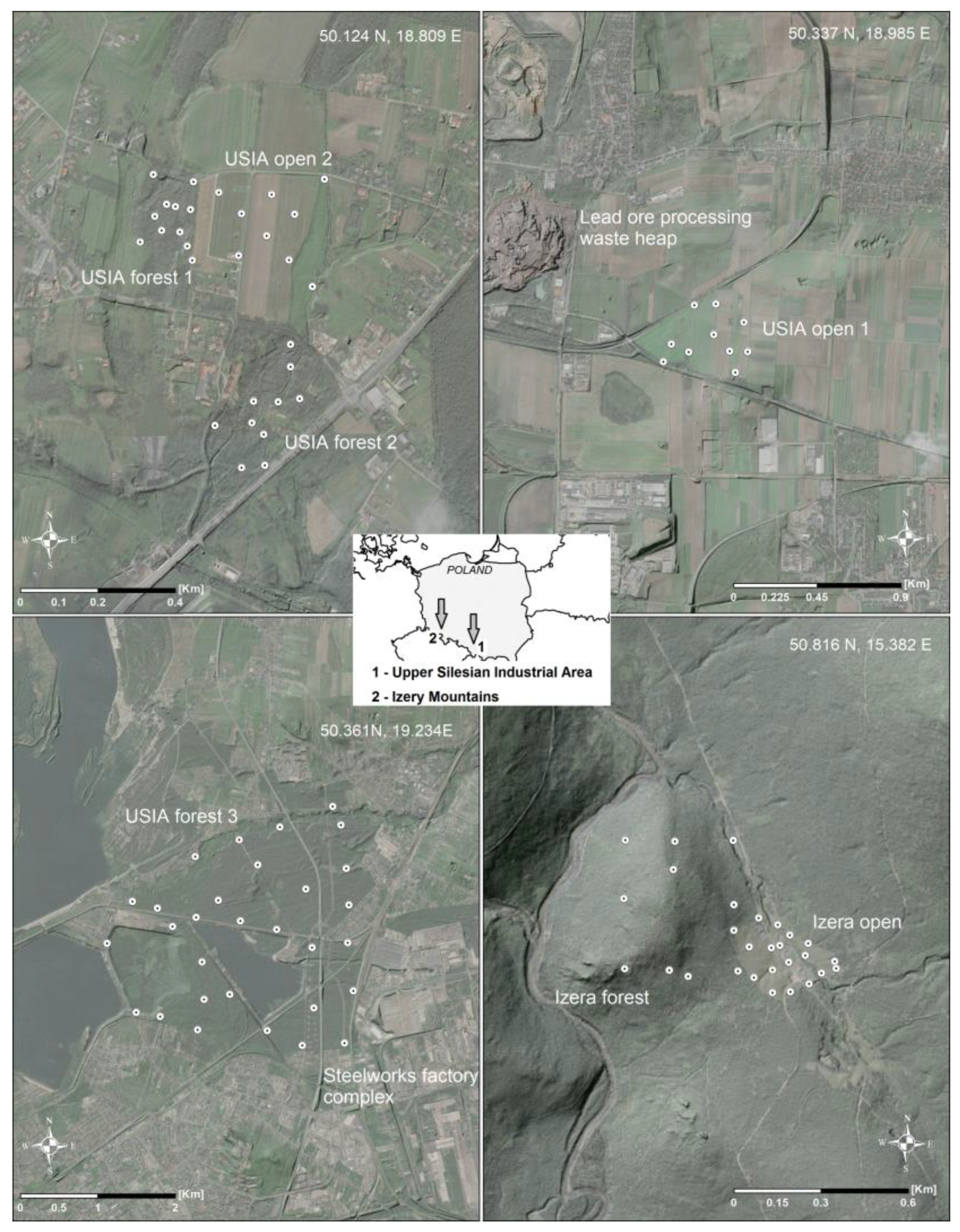
The area USIA open 1 (WGS84: 50.337° N, 18.985° E) was located in an arable field, adjacent from the south by the public roads, and was subjected to the direct pollution from nearby waste heap (about 600 m away to the south-west) of tailings from Pb-Zn ore processing factory (Figure 1) that contained significant amounts of Pb and Zn, Hg, Be, Cu, Ag, Se as well as rare earths. Dusts generated during the process of the sulphidation of the sulphides contained in deposited wastes were next transported by the wind to nearby areas. The geological bedrock of this study area included two geological formations: sands, silts and diluvial clays (Quaternary) in the eastern part, and dolomites and limestones (Middle Triassic) in the western part. In this study area, the dominant soils were brown leached and rainfall-glial soils developed of clay sands, loams, silt deposits and loams. No characteristic and undisturbed soil horizons were observed due to the fact that the field was still cultivated.

Study areas USIA open 2, USIA forest 1 and USIA forest 2 included one arable field and two adjacent forest areas, respectively (Figure 1). They were located (WGS84: 50.124˚ N, 18.809˚ E) in southern Poland, about 16 km south of the large Katowice agglomeration. The closest industrial emission source was the Laziska power plant, located about 2 km to the north-east of the study areas. The area USIA open 2 was an arable field, and the study area USIA forest 1 was located in a natural forest that was surrounded by arable fields. The dominant tree species were old black alder and young maple, oak and ash. The third study area, USIA forest 2, was located in a park, where the oldest trees were about 150 years old. Some parts of this park were overgrown with only weeds and shrubs. The geological bedrock of study areas USIA open 2, USIA forest 1 and USIA forest 2 were glacial sands and gravels (Quaternary). Dominant types of soils were brown leached and rainfall-glial soils developed of clay sands, loams, silt deposits and loams.

The study area USIA forest 3 (WGS84: 50.361° N, 19.234° E) was a large park located in the vicinity of steel plant called Katowice Metallurgical Complex (adjacent to the east). The predominant tree species were pine trees with some admixtures of deciduous species, such as birch and poplar. The deciduous trees grew mostly in the lower-lying and marshy places where sand exploitation reached the impermeable clayey bedrock. The geological bedrock of this study area was mostly glacial sand and gravel (Pleistocene), some aeolian sands in northern part, and in west-southern part valley bottoms muds (Holocene). The dominating soil type in this area was natural podzols and initial soils developed in the parts recultivated after former sand exploitation (mostly northern part of the study area).

The area Izera open and forest (WGS84: 50.816° N, 15.382° E) were located in the southwestern part of Poland, in the Izera Mountains. The area Izera open was exposed to the anthropogenic influence of a former glasswork that was active there between 18th and 19th century. When the glasswork was operational, waste management was rather non-existent, so in consequence significant volumes of waste were deposited in this area. As it was analyzed by Kowalczyk and Mazanek [24] in this part of Poland some ores, such as monacite, xenotile, apatite, containing REEs can be found, however in limited quantities. Part of the Izera region is commonly called the Black Triangle because of high pollution with industrial dusts emitted by numerous pollution sources in Poland, Germany, and Czechia [23]. Area Izera forest was located on a hill (about 870 m.a.s.l.) whose western, northwestern and southwestern parts of the slope were exposed to the long-range pollution from power plants in Poland, Germany, as well as Czechia [25]. In the direct vicinity of areas Izera forest and Izera open there were no active pollution sources. The major anthropogenic pressure was related to the long-range pollution from Czechia, and Germany. The geological bedrock of this region is mostly medium-grain granites, porphyry, coarse-grained in some places (Upper Carboniferous), local sands, gravels, and in some places muds of valley bottoms and floodplain terraces (Holocene). The soils of this area were acidic and leached brown soils developed from weathering of flysch rocks. The thickness of particular soil horizons was very low, and some of them were not fully developed.

2.2. Field and Laboratory Measurements

Measurements were performed in two phases. First, the soil cores were collected using a Humax sampler equipped with plastic tubes with a length of about 30 cm. It depended on soil conditions in particular study areas, but generally collected soil cores included organic horizon O, mineral horizon A, and a part of eluviated horizon E. In all study areas soil cores were collected from locations, that were away from the trunks of trees, to avoid the influence of effects related to washing industrial dust from tree trunks and branches.

Next, soil cores were used for in-profile magnetometric measurements that were performed in the laboratory with a use of the MS2C Bartington sensor (Bartington Instruments, Oxon, England) [26]. The result of magnetometric measurement was a distribution of κ values along the collected soil cores. The MS2C sensor has a working frequency of 0.565 kHz. The MS2C can be set to operate in two sensitivity ranges, namely 1.0 × 10⁻⁵ or 0.1 × 10⁻⁵ SI, and collected soil cores were measured with the sensitivity set to 0.1 × 10⁻⁵ SI. The spatial resolution of MS2C was equal to 2 cm.

After magnetometric measurements soil samples were air dried, homogenized, and sieved through 2 mm mesh to separate the soil skeleton and artifacts. From each collected soil core, one soil sample for chemical measurements was prepared. Next, about 250 mg of dried soil sample was digested using 50% (v/v) HNO₃. Each soil sample was then placed in a Teflon bottle, diluted to 108 mL, and transferred to 15 mL vials for ICP-MS (Elan DRC-e, PerkinElmer Inc., Waltham, MA, US) analysis of REEs concentration in soil.

2.3. Soil Pollution Indexes

Measured concentrations of REEs were used to calculate values of EF [27,28] and IG [28,29,30]. As was proposed by Krachler et al. [31] values EF of REEs were calculated in a reference to a concentration of Sc, accordingly to the formula:

$$EF=\frac{\left(\frac{M_{sample}}{S{c}_{sample}}\right)}{\left(\frac{M_{background}}{S{c}_{background}}\right)}$$

(1)

where: M_sample, M_background—measured and background concentration of selected element, Sc_sample, Sc_background—measured and background concentration of Sc.

IG reflects better the level of pollution rather than natural enrichment, as in the case of EF. However, it was decided to also use this indicator, because it was previously commonly used to assess the soil pollution [28]. IG was defined as:

$$IG={log}_2\frac{M_{sample}}{1.5\times M_{background}}$$

(2)

Table 3. Classes of IG and EF [27,28,29,30].

IG	Pollution Level	EF	Enrichment Level
0	Background	<1	No enrichment
0–1	No pollution	1–3	Minor enrichment
1–2	No pollution to moderate	3–5	Moderate enrichment
2–3	Moderate	5–10	Moderate to severe enrichment
3–4	Moderate to high	10–25	Severe enrichment
4–5	High	25–50	Very severe enrichment
-	-	>50	Extreme severe enrichment

summarizes the EF and IG classes that were used in further analyses to classify the level of soil pollution.

2.4. Classification of Collected Soil Cores

Using collected soil cores, the parameters of distributions of κ values in relation to the depth were measured with MS2C Bartington sensor and used to classify cores into six distinctive types. Out of the types specified by Magiera et al. [23] the following types were used in this study: A2, A3, and G (

Table 4. Types of κ distributions in soil profile and number of collected soil cores assigned to each type; the asterisk denotes the new types specified in this study.

Characteristics of the Distribution of Soil κ in Soil Profile	Type	Symbol Used	Number of Soil Cores
steep peak of κ in topsoil	Type A2	A2	52
wide peak of κ in topsoil	Type A3	A3	33
two similar peaks of κ at different depths *	-	TP	21
constant increase of κ with a depth	Type G	G	6
wide and flat peak of κ *	-	FL	24
wide and flat peak of κ with a noticeable subpeak of κ *	-	FLsub	27

).

2.5. Statistical Methods

Measured concentrations of REEs and calculated values of IG and EF were analyzed using selected statistical methods. Firstly, descriptive statistics, such as average, minimum, maximum, 25% and 75% quartiles, coefficient of variation, standard deviation, and skewness were calculated. Additionally, box-and-whisker plots were calculated, in order to graphically illustrate the variability of REEs concentrations and calculated values of IG and EF.

The hypothesis that the distributions of measured concentrations of REEs follow the normal distribution was tested using Shapiro–Wilk test. Average and median concentrations of REEs and calculated values of IG and EF were compared using selected statistical tests:

• Mann–Whitney test for comparing differences between average values of EF and IG index.
• Kruskal–Wallis H test for comparing differences between median values, with a hypothesis that all median values are equal versus hypothesis that there is at least one median that differs from the rest. This test was selected accordingly to the characteristics of the distributions of measured values, in particular different variances and in some cases lack of distribution normality.
• T-test for comparing average concentrations of REEs.

All statistical calculations were performed in the Statistica software, (version 10, StatSoft, Tulsa, OK, USA).

3. Results and Discussion

3.1. Concentrations of La, Ce, Pr, Nd and Sm in Soil

In first step measured concentrations of light REEs were used to calculate basic descriptive statistics (

Table 5. Descriptive statistics of concentrations of light REE: La, Ce, Pr, Nd and Sm in soil in study areas, as well as Sc concentration that was used to calculate EF and IG.

REE	Area	Number of Samples	Average	Min	Max	First Quartile	Third Quartile	Standard Deviation	Coefficient of Variation	Skewness
			(mg/kg)						(-)
La	Izera forest	14	19.36	11.25	30.94	14.01	22.02	5.79	29.93	0.36
	Izera open	34	19.85	5.82	28.93	17.01	23.00	4.63	23.31	−0.62
	USIA forest 1	12	10.77	1.82	21.08	8.40	12.24	4.76	44.21	0.29
	USIA forest 2	21	8.21	3.71	12.82	6.63	9.80	2.55	31.05	−0.00
	USIA forest 3	32	6.01	1.84	21.98	3.01	7.24	4.67	77.62	1.89
	USIA open 1	31	18.58	14.66	23.71	16.66	20.84	2.40	12.93	0.26
	USIA open 2	19	12.91	6.80	24.71	8.55	14.80	5.43	42.08	1.07
Ce	Izera forest	14	37.18	21.66	53.25	26.21	44.83	10.60	28.51	−0.27
	Izera open	34	41.13	11.12	61.81	34.10	47.19	10.24	24.91	−0.60
	USIA forest 1	12	22.62	3.71	41.29	19.85	24.82	8.76	38.75	−0.01
	USIA forest 2	21	16.70	7.39	27.41	12.82	19.76	5.54	33.16	0.23
	USIA forest 3	32	11.86	3.45	45.45	5.87	13.76	9.58	80.82	2.03
	USIA open 1	31	39.31	31.09	50.16	34.15	44.26	5.52	14.03	0.23
	USIA open 2	19	26.34	13.64	54.89	17.16	29.40	12.03	45.67	1.31
Pr	Izera forest	14	4.35	2.44	6.18	3.26	5.22	1.19	27.50	−0.36
	Izera open	34	4.71	1.35	7.16	3.98	5.33	1.13	24.02	−0.52
	USIA forest 1	12	2.59	0.45	5.14	1.82	2.97	1.16	44.64	0.33
	USIA forest 2	21	1.90	0.85	3.24	1.53	2.33	0.62	32.80	0.24
	USIA forest 3	32	1.35	0.40	5.04	0.68	1.55	1.06	78.05	1.98
	USIA open 1	31	4.37	3.49	5.73	3.80	4.95	0.62	14.10	0.37
	USIA open 2	19	3.00	1.56	6.07	1.99	3.33	1.31	43.77	1.20
Nd	Izera forest	14	16.09	9.41	22.55	12.22	19.03	4.22	26.24	−0.37
	Izera open	34	17.15	4.83	25.91	14.41	19.31	4.12	24.05	−0.60
	USIA forest 1	12	9.32	1.55	19.61	6.34	10.61	4.31	46.28	0.71
	USIA forest 2	21	6.96	3.16	11.68	5.52	8.37	2.27	32.68	0.25
	USIA forest 3	32	5.07	1.38	18.94	2.47	5.91	3.95	77.91	1.97
	USIA open 1	31	16.56	13.31	21.48	14.24	18.98	2.31	13.94	0.40
	USIA open 2	19	10.86	5.53	23.25	7.41	11.40	5.06	46.56	1.49
Sm	Izera forest	14	3.26	1.77	4.34	2.58	3.92	0.84	25.74	−0.47
	Izera open	34	3.44	0.93	5.33	2.77	3.94	0.86	24.84	−0.45
	USIA forest 1	12	1.72	0.30	3.82	1.16	2.00	0.86	49.92	0.88
	USIA forest 2	21	1.31	0.60	2.24	0.97	1.56	0.44	33.69	0.29
	USIA forest 3	32	0.97	0.26	3.60	0.44	1.17	0.76	78.60	1.92
	USIA open 1	31	3.14	2.42	4.18	2.76	3.64	0.47	14.93	0.30
	USIA open 2	19	1.93	0.98	4.81	1.23	2.00	1.06	55.09	1.87
Sc	Izera forest	14	3.07	2.03	5.15	2.31	3.60	0.93	30.40	1.10
	Izera open	34	3.40	1.87	5.02	2.75	4.06	0.86	25.38	0.14
	USIA forest 1	12	2.68	0.70	5.11	1.81	3.35	1.24	46.12	0.46
	USIA forest 2	21	1.87	0.76	3.14	1.23	2.17	0.71	37.87	0.17
	USIA forest 3	32	1.41	0.48	4.21	0.69	1.71	0.99	70.09	1.43
	USIA open 1	31	4.02	2.51	6.96	3.33	4.72	0.93	23.11	1.08
	USIA open 2	19	2.12	1.13	7.86	1.30	2.02	1.53	72.01	3.31

). Statistics were calculated separately for concentrations of La, Ce, Pr, Nd, and Sm in soil, and for each study area.

The lowest average concentrations of REEs were observed in the area USIA forest 3, which was the largest study area, located in the urban park with neighboring steelworks and urban areas (see Figure 1). However, it is important to notice that some high concentrations of REEs were also observed in this area that contributed to the highest right skewness and high values of coefficient of variation. A similar type of strongly right-skewed distribution was observed in the area USIA open 2 that was located in the direct vicinity of the waste heap of lead ore postprocessing (see Figure 1). In this case, the observation of high maximum concentrations of REEs and the associated strong right skewness could be explained by a large stream of dusts that were wind-blown from weathering waste heap. In other forested areas (USIA forest 1 and 2), distributions of measured REEs concentrations were much less skewed, and one of the reasons may be that these areas were much smaller and additionally much more homogeneous in terms of anthropogenic pressure. It is also important to notice that in forested areas, trees and other plants can play some role in accumulating REEs [32,33,34]. However, to precisely verify this hypothesis it would be necessary to perform more detailed and focused studies that are beyond the scope of this study.

In the Izera Mountains the distributions of measured REEs concentrations had interesting characteristics. Although the highest concentrations of REEs in soil were observed in this region, the distributions were not right skewed, which is generally observed in the case of anthropogenically contaminated soils. Contrary, a left-hand skewness was observed, which, however, can be explained by high natural concentration of ores rich in REEs in this region.

After the analysis of distributions of measured REEs concentrations in soil with the Shapiro–Wilk test (with α = 0.05), it was concluded there was no basis to reject the hypothesis that the distributions of La, Ce, Pr, Nd and Sm follow the normal distribution in areas: Izera open, Izera forest, USIA open 1, USIA forest 1 and 2. Only in the case of areas USIA open 2 and USIA forest 3 the distributions of REEs were so strongly right-skewed that it could not be assumed that they are close to the normal distribution.

The results of the comparison of average concentrations of La, Ce, Pr, Nd and Sm in all study areas suggested that they could be divided into three groups: forested areas (USIA forest 1, 2 and 3) where the measured REEs concentrations were the lowest, open areas where the measured REEs concentrations were moderate to high (USIA open 1 and 2), and mountain areas where the highest REEs concentrations were observed (Izera forest and open). As it was analyzed using t-test for comparing average concentrations of REEs (with α = 0.05), the differences between average concentrations of La, Ce, Pr, Nd, Sm measured in soils of these three groups were statistically significant.

Next, measured concentrations of La, Ce, Pr, Nd, Sm were used to calculate the IG and EF, as described in the Materials and methods section, using the background concentrations that were determined in previous studies [1]: La = 2.70 mg/kg, Ce = 5.50 mg/kg, Pr = 0.70 mg/kg, Nd = 2.30 mg/kg, Sm = 0.40 mg/kg, and Sc = 0.70 mg/kg. Naturally, it could be advantageous to use local background concentrations of REEs. However, it would be difficult to determine the background values in relatively small study areas that were additionally located in industrial regions. Determination of the background would require performing measurements in areas without a significant anthropogenic impact, and it was rather beyond the scope of this study. Apart from the EF and IG values, at the beginning of the paper concentrations of REEs were analyzed, and the results showed consistency with EF and IG (highest values in mountains, lower in open areas, lowest in forests). It was an additional suggestion that the used background values were sufficiently representative.

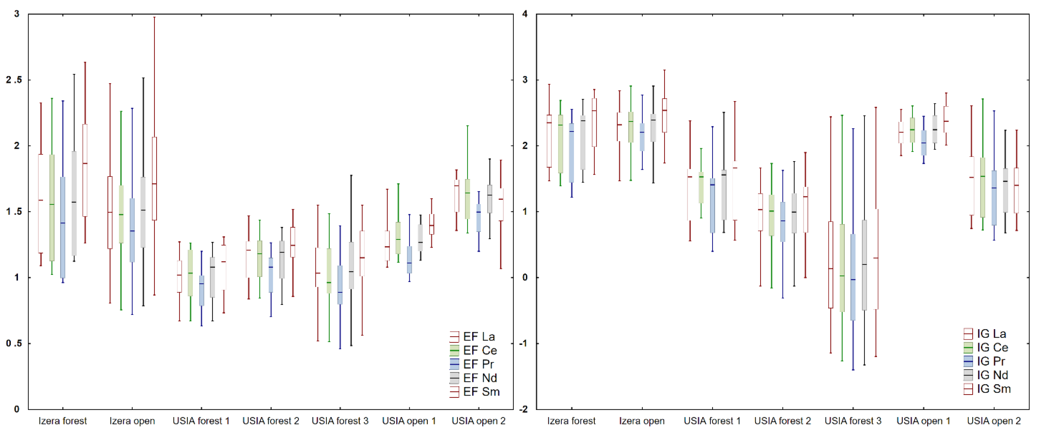
As can be noticed in Figure 2, the highest EF values were observed in areas located in the Izera mountains (areas Izera forest and Izera open). Simultaneously, the EF values in these areas were characterized by a relatively large spread, from about 0.6 to almost 3. Such observations suggest that only in areas Izera forest and Izera open concentrations of La, Ce, Sa, Nd and Pr were slightly elevated in relation to the natural background, which may have been due to the fact that REEs-rich minerals commonly occur in this region. As it can be observed in Figure 2, in USIA areas the EF values were significantly lower than in Izera Mountains, and the lowest EF values (with average equal about to 1) were observed in forested areas that might suggest negligible soil enrichment with analyzed REEs.

The highest IG values were observed, similarly like in the case of EF, in Izera region. However, almost as high values of IG were also observed in arable fields (USIA open 1 and 2). In these regions average IG index greater than two suggested moderate pollution (Table 3). Comparing IG values calculated for two arable fields (USIA open 1 and 2), it was clearly noticeable that higher IG values were observed in the area USIA open 1. This area was located in the direct vicinity of waste heap of lead ore processing factory (Figure 1), so it can be assumed that it was a reason of increased IG values.

The lowest IG values were observed in forested areas, additionally in the area USIA forest 3 these values were characterized by a very large spread from −1 to almost 3 (see Figure 2). This effect was due to the fact that the area USIA forest 3 was the largest, soil conditions were the most complex from all studied areas, and some parts of this area were recultivated after former sand exploitation in the past.

After comparing the box-and-whisker plots of EF and IG, the mean values of these indexes were additionally compared using the Mann-Whitney test (with α = 0.05). The results of this test confirmed that the average values of EF and IG that were calculated for areas located in Izera mountains were significantly higher than those measured in other areas. Similar statistically significant differences were observed between average values of EF and IG index of forested (USIA forest 1, 2, and 3) and open areas (USIA open 1 and 2).

To summarize, the highest values of EF index were observed in the Izera mountains (Izera forest and Izera open), significantly lower in arable fields (USIA open 1 and 2) and the lowest in forests (USIA forest 1, 2 and 3). The differences between EF values of arable fields and forested areas were low (see Figure 2). The highest IG values were observed in areas Izera forest and Izera open, almost as high in arable fields (USIA open 1 and 2) and the lowest in forests (USIA forest 1, 2 and 3).

It can also be noticed that the differences between EF values of arable fields and forested areas were slightly less pronounced than in the case of IG (see Figure 2). However, it should be taken into account that the EF values were calculated in relation to the concentration of Sc, and in arable soils much higher soils concentration of Sc (Table 1) were measured.

3.2. Analysis of La-to-REEs Ratios

As it was previously proposed by Yusupov et al. [35], the ratios of La concentration to the concentrations of Ce, Pr, Nd and Sm were also analyzed, in order to observed if the REEs concentrations in soils could be of natural or anthropogenic origin. Corresponding ratios of EF of La to EF of Ce, Pr, Nd and Sm were also calculated and analyzed.

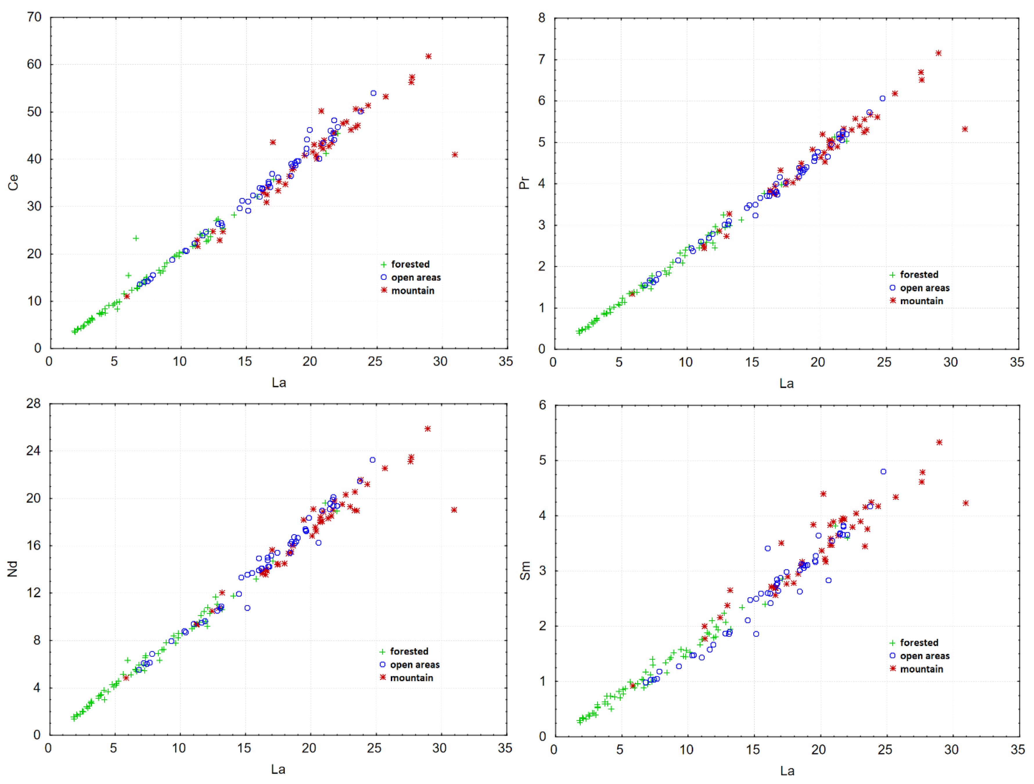
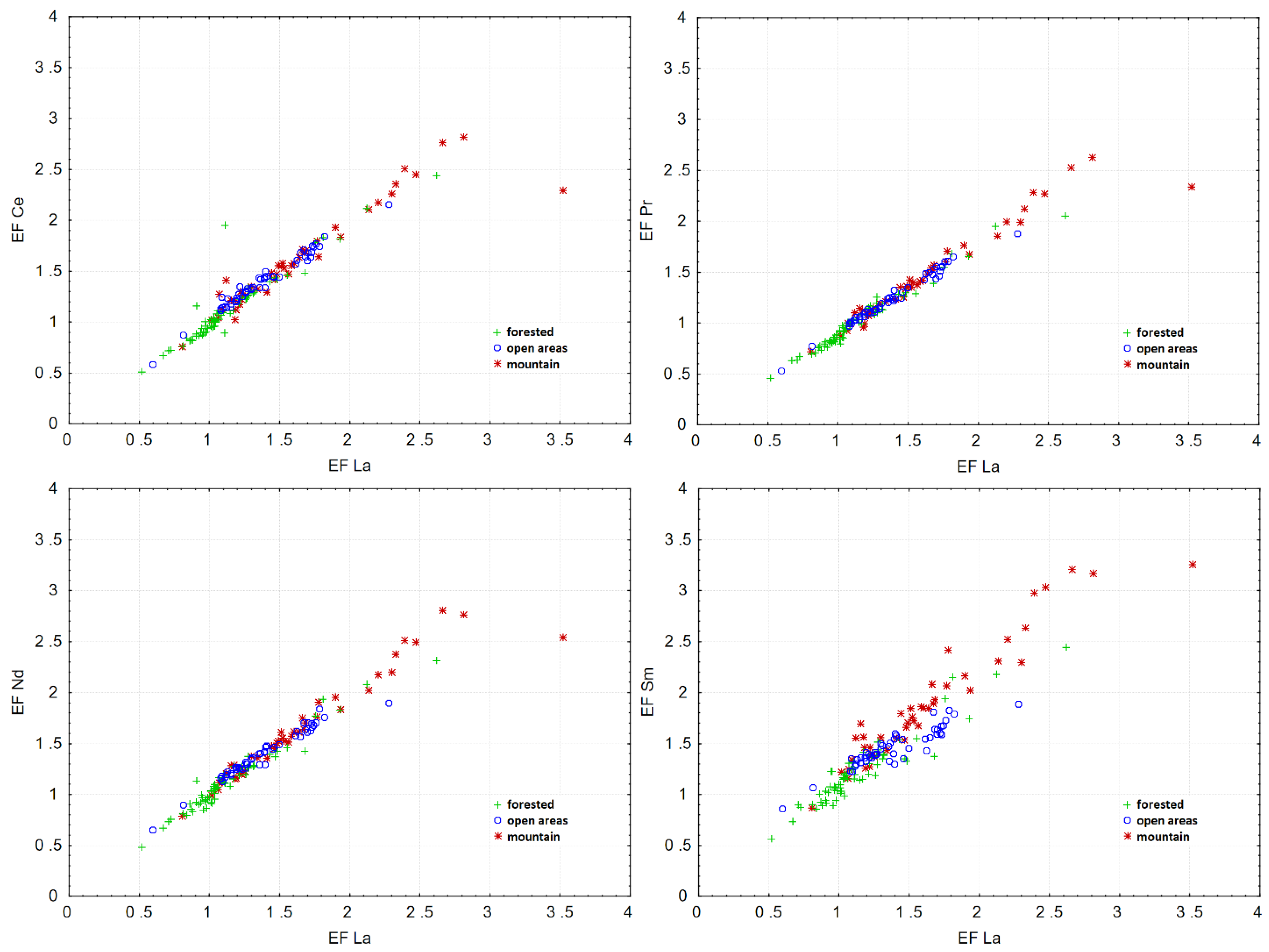
As shown in Figure 3 and Figure 4, the relationship between concentration of La and concentrations of other light REEs was almost linear. There was a clear distinction between the group of values measured in forested and in mountain areas. In the scatterplots, the points related to the values measured in forested areas were much closer to the origin compared to those related to the values measured in mountain areas. This could be due to the fact that REEs concentrations in forested areas were much lower than those measured in mountain areas (compare Table 5). The third group of points in the scatterplots (open areas) was spread at the boundary between the groups of points from forested and mountain areas, partially overlapping these two groups. The explanation for this was related to the fact that the studied open areas included regions where high REEs concentrations were measured (Izera open and USIA open 1), as well as the USIA open 2 area, where the measured REEs concentrations were comparable to those observed in forested areas.

Analyzing the slope of scatter plots in the Figure 3, it could be concluded that the ratio of La concentration to the Ce concentration was equal to almost 2:1. In the case of Pr, Nd, and Sm the ratios were lower than 1, and were approximately equal to 0.2, 0.9, 0.2 for Pr, Nd, Sm, respectively.

As it can be observed on the scatterplots of EF values in the Figure 4, the ratios of EF of La to EF of Ce, Pr, Nd and Sm were practically all equal to 1:1. In contrast to the absolute REEs concentration, the EF values were calculated in a relation to the background values of individual REEs and Sc. It can be observed in Figure 4 that the points of the scatterplots were centered around a 45 degrees line. The conclusion from this observation could be that the soils of the studied areas were similarly enriched in La, Ce, Pr, Nd, and Sm, and the mutual relations of enrichment with these elements were very similar.

It was also observed that the cloud of points in all scatterplots (Figure 3 and Figure 4) was spreading as the concentrations of REEs or EF values were increasing. It may suggest that the dependence of La and Ce, Pr, Nd and Sm ratios was almost linear for low REEs concentrations in soil, whereas for the higher ones these correlations could deviate from linear. An additional explanation for this observation may be that high measured REEs concentrations were associated with increased soil pollution or (in the area USIA 1) with a combination of soil pollution and higher natural concentrations of REEs (in the area Izera mountains).

3.3. Grouping of EF Values Depending on the Type of κ Distribution in Collected Soil Cores

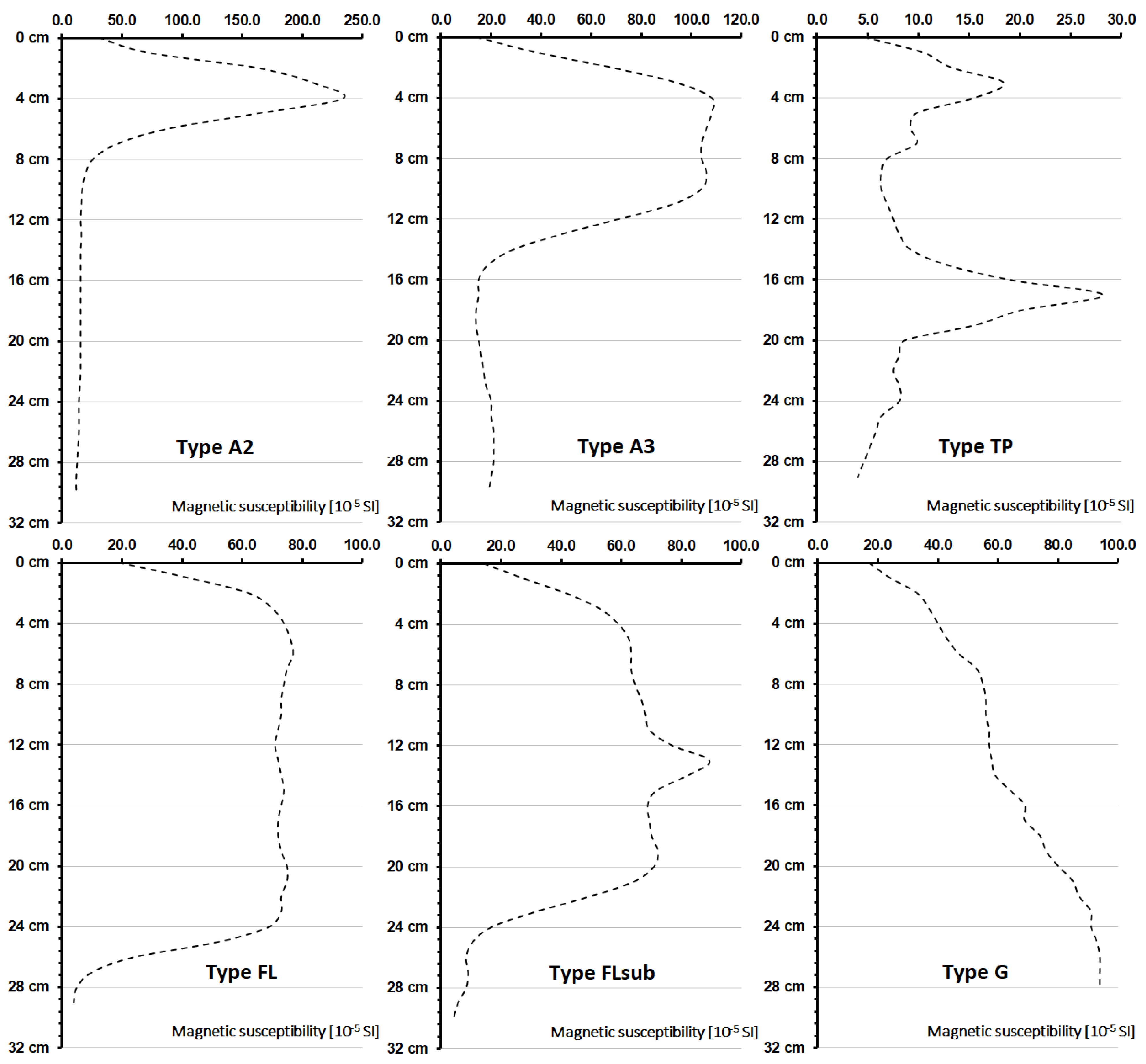
Distributions of κ measured in collected soil cores were grouped into six types, and examples of each type were presented in Figure 5.

Types A2 and A3 refer to distributions of κ with a visible peak of κ values at a depth of several centimeters. These types are very closely related to potential soil pollution, and the location of peaks at such depth is associated with the accumulation of TMPs in organic soil horizons. The main difference between the A2 and A3 types is in the peak of the maximum κ values (see Figure 5). In type A2 the peak is narrow and located at the depth of about 3 cm, while in type A3 the peak is wide and covers a much thicker soil layer (about 10 cm). As it was previously analyzed, the A3 type was also more common for soils developed in deciduous forests [23]. The type marked as type G, was a profile in which a continuous increase of κ was observed along with the depth in soil profile. This type is usually observed in locations with strong lithogenic influence.

In addition to the three above-described types of distribution, three additional types were specified, and denoted by TP, FL, and FLsub (Figure 5 and Table 4). These types were selected after initial analysis of κ distributions measured in collected soil cores. The most characteristic feature of the TP type was the occurrence of two noticeable and comparable peaks of κ values at different depths in soil core. This type was specified because in the area Izera open intensive industrial activity was carried out in the past. As a result of this activity, some amounts of waste might have been deposited in the area where the soil samples were taken, which is the explanation for the occurrence of a second peak of κ values in the deeper parts of the collected soil cores [23].

The last type, FL, was the type observed mainly in arable areas. In this type of distribution κ values were almost constant throughout the entire soil core (Figure 5). In the similar type FLsub, additionally, one small but well-visible peak of κ, was observed at the depth of about 12 to 20 cm. Significant numbers of FLsub profiles were observed in the arable field located in the direct distance to the waste heap (USIA open 1).

Apart from the differences in the shape of individual profiles, significant differences in κ values were also observed. In the case of the type A2, which is the most characteristic for polluted soils, measured κ values were almost equal to 250 × 10⁻⁶ SI. In the case of the A3, FL and FLsub profiles, the κ values were about two times lower. The lowest values, up to 30 × 10⁻⁶ SI, were observed for TP profiles from the Izera Mountains region. In the region where study areas were located (Upper Silesian Industrial Area) so far, extensive magnetometric studies were performed [17,36,37] that included measurements of κ on the soil surface and in soil profile. The results of these measurements showed that the κ values ranged from about 20 × 10⁻⁵ SI for unpolluted soils to above 100 × 10⁻⁵ SI for polluted soils. Extremely polluted soils were characterized by κ equal to over several hundred 10⁻⁵ SI.

Next, collected soil samples were grouped according to the type of area (mountain, open and forested areas) and additionally according to the type of κ distribution that was observed in collected soil cores. The resulting groups included following number of soil samples:

• forested area: 36 A2, 16 A3, 3 G, 10 TP.
• open area: 20 FL, 27 FLsub, 3 G.
• mountain area: 16 A2, 17 A3, 4 FL, 11 TP.

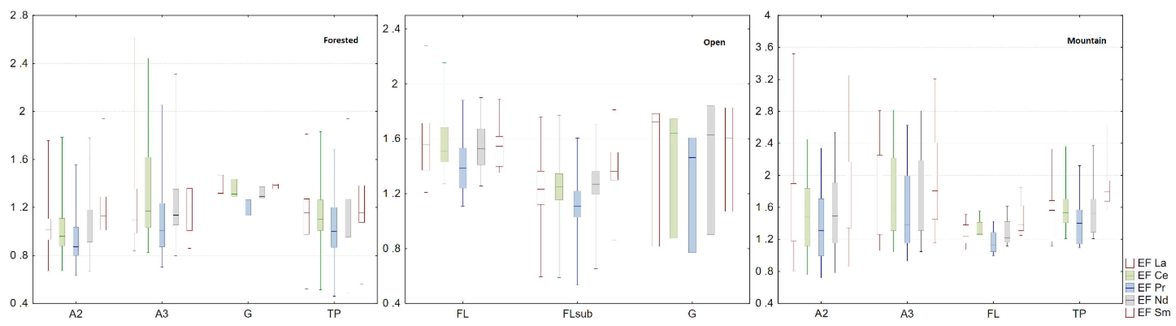
Further analyses were based only on the values of EF, because as suggested in the literature that index is a more suitable than IG for analyzing concentrations of REEs [31]. Box-and whisker plots of EF of REEs were calculated, as presented in Figure 6.

In forested areas, EF values from group G were a bit higher comparing to the values of EF from groups A2, A3 and TP, as it can be observed on box-and-whisker plots (Figure 6). Taking into account the fact that in the case of the G type, the natural lithogenic effect is dominant [23], while in the case of types A2, A3 and TP it is the anthropogenic effect, it can be supposed that in forested areas the concentrations of REEs in soil could, to some extent, be conditioned by the natural properties of the soil and geological substrata.

As it could be expected, in open areas the dominant types of κ distribution were the FL and FLsub ones. Soils of cultivated arable fields are generally severely disturbed and usually no characteristic soil horizons are observed. However, visible differences were observed. The distribution of EF values in FLsub group had slightly larger range and interquartile range. It is possible that this greater spread of EF values could be caused by the increased accumulation of REEs in thin soil layer at the depth of about 12–16 cm, where small but distinct peak of the κ was observed in soil cores of FLsub type (see Figure 5, FLsub profiles). FLsub profiles were observed mainly in the area USIA open 1, and it was the dominant type observed in this area. Possibly, this small peak of the κ (and possibly a soil layer of increased REEs accumulation) was caused by pollution from nearby heap of lead ore post-processing.

In mountain areas, box-and-whisker plots of EF values (Figure 6) for the group A2 and A3 were similar, both in terms of value and spread. Only in the case of the group A2 slightly higher number of high EF values, above 75% quartile, were observed. As can be seen in Figure 6, despite EF values for all REEs of the TP group were similar to those observed in groups A2 and A3, the distributions of EF values of the TP group were characterized by a significant right-skewness (see boxplots in Figure 6), which is characteristic for strong anthropogenic pollution. It is important to notice that the TP group reflected the historical activity of the glassworks in this place, especially wastes that were deposited in this area, what was detected using magnetometric methods as the secondary peak of κ values (see plot TP in Figure 5).

Using the Kruskal–Wallis H and median tests, EF values grouped according to the type of κ distribution, were also compared. Following profile types were included in the analysis: A2, A3, TP, FL, and FLsub. The type G was not included in Kruskal–Wallis H and median tests because of the too small number of EF values in this group.

The result of tests, presented in

Table 6. Results of Kruskal–Wallis H test and median test in brackets. p-values for test with a hypothesis that all median EF values of different types of soil profile are equal versus hypothesis that there is at least one median that differs from the rest.

Area Type	κ Profile Type	EF La	EF Ce	EF Pr	EF Nd	EF Sm
Forested	A2, A3, TP	0.16 (0.11)	0.02 (0.01)	0.10 (0.11)	0.13 (0.03)	0.57 (0.84)
Open	FL, FLsub	0.01 (0.01)	0.01 (0.01)	0.01 (0.01)	0.01 (0.01)	0.01 (0.01)
Mountain	A2, A3, TP	0.71 (0.84)	0.55 (0.59)	0.72 (0.83)	0.65 (0.74)	0.74 (0.84)

, suggest that statistically significant differences were found between median EF values of all REEs that were measured in groups FL and FLsub in open areas. The κ distributions of the FL type were mainly observed in the area USIA open 1 whereas the FL type in USIA open 2. The major difference between these two areas was that USIA open 1 was located in the direct vicinity of pollution source (lead ore postprocessing waste heap—see Figure 1), and it could be assumed that the observed significant differences can be attributed to this anthropogenic pollution. In forested areas the significant differences were found only for median EF of Ce and median EF of Nd. In mountain areas no statistically significant differences between median EF values measured in soil profiles A2, A3, TP for all REEs were found.

4. Conclusions

The results of chemical and magnetometric measurements of REEs concentrations in various areas that were subjected to the anthropogenic pollution provided different but complementary information which allowed to obtain deeper insight on REEs concentrations in soils of studied areas. Among others, it was found that the average concentrations of La, Ce, Pr, Nd, Sm measured in open, forested, and in mountain areas were statistically different, whereas no significant differences were found between average REEs concentrations of particular study areas in each of these three types of area.

It was also found that the ratios of La concentration to the concentrations of Ce, Pr, Nd, Sm calculated for forest, open and mountain areas formed two separate clusters on the scatter plots. There was a clear distinction between groups of values measured in forested and in mountain areas. Points related to values measured in open areas were spread at the boundary between these two groups, partially overlapping them.

Moreover, the study demonstrated the existence of the pronounced relationship between the type of a magnetic susceptibility distribution in a soil core (A2, A3, G, FL, FLsub, TP) and measured REEs (La, Ce, Pr, Nd, Sm) concentrations, as well as their EF. Apart from those described in the literature, three additional types of a magnetic susceptibility distribution in a soil core were determined in this study, denoted by TP, FL, and FLsub. These types were characteristic for post-industrial areas (TP) and arable areas (FL, and FLsub).

Such results suggest that fly ashes emitted from industrial sources and then deposited on the soil surface can include TMPs and REEs compounds that have magnetic properties detectable with magnetometric sensors.

The results of a use of soil magnetometry for an analysis of REEs concentrations in soil are promising, but may require further, detailed studies of industrial dust composition, e.g., the microscopic examination of REEs compounds in the dust, and associated with them magnetic TMP phases. Such studies are far beyond the scope of this work because the interrelations between TMPs and REEs in dusts might be very complex.

References

- Ramos, S.J.; Dinali, G.S.; Oliveira, C.; Martins, G.C.; Moreira, C.G.; Siqueira, J.O.; Guilherme, L.R.G. Rare Earth Elements in the Soil Environment. Curr. Pollut. Rep. 2016, 2, 28–50. [Google Scholar] [CrossRef] [Green Version]
- Salminen, R.; Batista, M.J.; Bidovec, M.; Demetriades, A.; De Vivo, B.; De Vos, W.; Duris, M.; Gilucis, A.; Gregorauskiene, V.; Josip, H.; et al. Geochemical Atlas of Europe. Part 1: Background Information, Methodology and Maps; Geological Survey of Finland: Espoo, Finland, 2005; ISBN 951-690-921-3. [Google Scholar]
- Aide, M.T.; Aide, C. Rare Earth Elements: Their Importance in Understanding Soil Genesis. ISRN Soil Sci. 2012, 2012, 1–11. [Google Scholar] [CrossRef] [Green Version]
- Cao, X.; Chen, Y.; Wang, X.; Deng, X. Effects of redox potential and pH value on the release of rare earth elements from soil. Chemosphere 2001, 44, 655–661. [Google Scholar] [CrossRef]
- Ran, Y.; Liu, Z. Adsorption and desorption of rare earth elements on soils and synthetic oxides. Acta Sci. Circumst. 1993, 13, 287–293. [Google Scholar]
- Beckwith, R.; Bulter, J. Aspects of the chemistry of soil organic matter. In Soils, an Australian Viewpoint; Division of Soils; CSIRO: Canberra, Australia, 1993. [Google Scholar]
- Adamczyk, Z.; Komorek, J.; Białecka, B.; Nowak, J.; Klupa, A. Assessment of the potential of polish fly ashes as a source of rare earth elements. Ore Geol. Rev. 2020, 124, 103638. [Google Scholar] [CrossRef]
- Zhang, S.; Shan, X.-Q. Speciation of rare earth elements in soil and accumulation by wheat with rare earth fertilizer application. Environ. Pollut. 2001, 112, 395–405. [Google Scholar] [CrossRef]
- Fabijańczyk, P.; Zawadzki, J.; Magiera, T. Towards magnetometric characterization of soil pollution with rare earth elements in industrial areas of Upper Silesian Industrial Area, southern Poland. Environ. Earth Sci. 2019, 78, 1–12. [Google Scholar] [CrossRef] [Green Version]
- Cao, L.; Appel, E.; Hu, S.; Yin, G.; Lin, H.; Rosler, W. Magnetic response to air pollution recorded by soil and dust-loaded leaves in a changing industrial environment. Atmos. Environ. 2015, 119, 304–313. [Google Scholar] [CrossRef]
- Petrovský, E.; Kapička, A.; Jordanova, N.; Knab, M.; Hoffmann, V. Low-field magnetic susceptibility: A proxy method of estimating increased pollution of different environmental systems. Environ. Earth Sci. 2000, 39, 312–318. [Google Scholar] [CrossRef]
- Spiteri, C.; Kalinski, V.; Rosler, W.; Hoffman, V.; Appel, E. Magnetic Screening of Pollution Hotspots in the Lausitz Area, Eastern Germany: Correlation Analysis Between Magnetic Proxies and Heavy Metal Concentration in Soil. Environ. Geol. 2005, 49, 1–9. [Google Scholar] [CrossRef]
- Fürst, C.H.; Lorz, C.; Makeschin, F. Testing a Soil Magnetometry Technique in a Highly Polluted Industrial Region in North-Eastern Germany. Water Air Soil Poll. 2009, 202, 33–43. [Google Scholar] [CrossRef]
- Łukasik, A.; Szuszkiewicz, M.; Magiera, T. Impact of artifacts on topsoil magnetic susceptibility enhancement in urban parks of the Upper Silesian conurbation datasets. J. Soils Sediments 2015, 15, 1836–1846. [Google Scholar] [CrossRef]
- Fabijańczyk, P.; Zawadzki, J.; Magiera, T. Magnetometric assessment of soil contamination in problematic area using empirical Bayesian and indicator kriging: A case study in Upper Silesia, Poland. Geoderma 2017, 308, 69–77. [Google Scholar] [CrossRef]
- Zawadzki, J.; Fabijańczyk, P.; Magiera, T.; Rachwał, M. Micro-scale spatial correlation of magnetic susceptibility in soil profile in forest located in industrial area. Geoderma 2015, 249–250, 61–68. [Google Scholar] [CrossRef]
- Zawadzki, J.; Szuszkiewicz, M.; Fabijańczyk, P.; Magiera, T. Geostatistical discrimination between a long-range and short-range soil pollution using field magnetometry. Chemosphere 2016, 164, 668–676. [Google Scholar] [CrossRef] [PubMed]
- Yang, P.; Drohan, P.J.; Yang, M. Patterns in soil contamination across an abandoned steel and iron plant: Proximity to source and seasonal wind direction as drivers. Catena 2020, 190, 104537. [Google Scholar] [CrossRef]
- Chaparro, M.A.E.; Nuñez, H.; Lirio, J.M.; Gogorza, C.S.G.; Sinito, A.M. Magnetic screening and heavy metal pollution studies in soils from Marambio Station, Antarctica. Antarct. Sci. 2007, 19, 379–393. [Google Scholar] [CrossRef]
- Yang, P.G.E.J.; Yang, M. Identification of Heavy Metal Pollution Derived From Traffic in Roadside Soil Using Magnetic Susceptibility. Bull. Environ. Contam. Toxicol. 2017, 98, 837–844. [Google Scholar] [CrossRef]
- Marié, D.C.; Chaparro, M.A.E.; Gogorza, C.S.G.; Navas, A.; Sinito, A.M. Vehicle-derived emissions and pollution on the road autovia 2 investigated by rock-magnetic parameters: A case study from Argentina. Stud. Geophys. Geod. 2010, 54, 135–152. [Google Scholar] [CrossRef] [Green Version]
- Fabijańczyk, P.; Zawadzki, J.J.; Magiera, T.; Szuszkiewicz, M. A methodology of integration of magnetometric and geochemical soil contamination measurements. Geoderma 2016, 277, 51–60. [Google Scholar] [CrossRef]
- Magiera, T.; Strzyszcz, Z.; Kapicka, A.; Petrovsky, E. Discrimination of lithogenic and anthropogenic influences on topsoil magnetic susceptibility in Central Europe. Geoderma 2006, 130, 299–311. [Google Scholar] [CrossRef]
- Kowalczyk, J.; Mazanek, C. Metale Ziem Rzadkich i ich Związki; Wydawnictwa Naukowo-Techniczne: Warsaw, Poland, 1989. (In Polish) [Google Scholar]
- Strzyszcz, Z.; Magiera, T. Magnetic susceptibility of forest soils in Polish—German border area. Geol. Carpath. 1998, 49, 241–242. [Google Scholar]
- Dearing, J.A. Environmental Magnetic Susceptibility: Using the Bartington MS2 System; Chi Publishing: Kenilworth, UK, 1994. [Google Scholar]
- Loska, K.; Cebula, J.; Pelczar, J.; Wiechuła, D.; Kwapuliński, J. Use of enrichment, and contamination factors together with geoaccumulation indexes to evaluate the content of Cd, Cu, and Ni in the Rybnik Water Reservoir in Poland. Water Air Soil Pollut. 1997, 93, 347–365. [Google Scholar] [CrossRef]
- Reimann, C.; De Caritat, P. Intrinsic flaws of element enrichment factors (EFs) in environmental geochemistry. Environ. Sci. Technol. 2000, 34, 5084–5091. [Google Scholar] [CrossRef]
- Birch, G.F. A Scheme for assessing human impacts on coastal aquatic environments using sediments. In Coastal GIS: An Integrated Approach to Australian Coastal Issues; Woodcoffe, C.D., Furness, R.A., Eds.; Wollongong University Papers in Center for Maritime Policy: Wollongong, Australia, 2003; Volume 14. [Google Scholar]
- Sutherland, R.A. Bed sediment-associated trace metals in an urban stream, Oahu, Hawaii. Environ. Earth Sci. 2000, 39, 611–627. [Google Scholar] [CrossRef]
- Krachler, M.; Mohl, C.; Emons, H.; Shotyk, W. Two thousand years of atmospheric rare earth element (REE) deposition as revealed by an ombrotrophic peat bog profile, Jura Mountains, Switzerland. J. Environ. Monit. 2002, 5, 111–121. [Google Scholar] [CrossRef]
- Tyler, G. Rare earth elements in soil and plant systems—A review. Plant Soil 2004, 267, 191–206. [Google Scholar] [CrossRef]
- Kovarikova, M.; Tomaskova, I.; Soudek, P. Rare earth elements in plants. Biol. Plant. 2019, 63, 20–32. [Google Scholar] [CrossRef]
- William, A.; Thomas, W.A. Accumulation of rare earths and circulation of cerium by mockernut hickory trees. Can. J. Bot. 1975, 53, 1159–1165. [Google Scholar]
- Yusupov, D.V.; Baranovskaya, N.V.; Robertus, Y.V.; Radomskaya, V.I.; Pavlova, L.M.; Sudyko, A.F.; Rikhvanov, L.P. Rare earth elements in poplar leaves as indicators of geological environment and technogenesis. Environ. Sci. Pollut. Res. 2020, 27, 27111–27123. [Google Scholar] [CrossRef]
- Rachwał, M.; Magiera, T.; Bens, O.; Kardel, K. Correlations between Soil Magnetic Susceptibility and the Content of Particular Elements as a Reflection of Pollution Level, Land Use and Parent Rocks; EGU General Assembly of European Geosciences Union: Vienna, Austria, 2015. [Google Scholar]
- Magiera, T.; Strzyszcz, Z.; Rachwał, M. Mapping particulate pollution loads using soil magnetometry in Urban forests in the Upper Silesia Industrial Region, Poland. For. Ecol. Manag. 2007, 248, 36–42. [Google Scholar] [CrossRef]
Figure 1.
Location of study areas; locations of soil cores collection were marked with white circles; base maps: LIDAR (Light Detection and Ranging) map and orthophoto map (Esri).
Figure 2.
Box and whisker plots (whiskers: min-max, box: upper and lower quartile, line: median) of IG and EF of light REEs, La, Ce, Pr, Nd, and Sm.
Figure 3.
Scatterplots of ratios La to: Ce, Pr, Nd and Sm concentrations for forested, open, and mountain areas; the points on the scatterplots were marked depending on the area, where the measurements was taken: forested areas by crosses (USIA forest 1, 2, and 3), open areas by circles (USIA open 1 and 2), and mountain areas by stars (Izera open and Izera forest).
Figure 4.
Scatterplots of ratios EF La to: EF Ce, EF Pr, EF Nd and EF Sm for forested, open, and mountain areas; the points on the scatterplots were marked depending on the area, where the measurements was taken: forested areas by crosses (USIA forest 1, 2, and 3), open areas by circles (USIA open 1 and 2), and mountain areas by stars (Izera open and Izera forest).
Figure 5.
Types of κ distribution in soil profile that were determined on the basis of collected soil cores.
Figure 6.
Box-and-whisker plots (whiskers: min-max, box: upper and lower quartile, line: median) of EF of: La, Ce, Pr, Nd, and Sm for different types of κ distribution in soil profile, grouped by the area type: forested, open, mountain; lack of whiskers in plots for type G results from low number of soil cores in these groups (only 3 per group)