Multi-Platform, High-Resolution Study of a Complex Coastal System: The TOSCA Experiment in the Gulf of Trieste

Abstract

Although small in size, the Gulf of Trieste (GoT), a marginal coastal basin in the northern Adriatic Sea, is characterized by very complex dynamics and strong variability of its oceanographic conditions. In April–May 2012, a persistent, large-scale anticyclonic eddy was observed in the GoT. This event was captured by both High Frequency Radar (HFR) and Lagrangian drifter observations collected within the European MED TOSCA (Tracking Oil Spill and Coastal Awareness) project. The complexity of the system and the variety of forcing factors constitute major challenges from a numerical modeling perspective when it comes to simulating the observed features. In this study, we implemented a high-resolution hydrodynamic model in an attempt to reproduce and analyze the observed basin-wide eddy structure and determine its drivers. We adopted the Massachusetts Institute of Technology General Circulation Model (MITgcm), tailored for the GoT, nested into a large-scale simulation of the Adriatic Sea and driven by a tidal model, measured river freshwater discharge data and surface atmospheric forcing. Numerical results were qualitatively and quantitatively evaluated against HFR surface current maps, Lagrangian drifter trajectories and thermohaline data, showing good skills in reproducing the general circulation, but failing in accurately tracking the drifters. Model sensitivity to different forcing factors (wind, river and tides) was also assessed.

1. Introduction

Integrated coastal observing systems are useful tools both for studying the dynamics of the marine environment and for operational applications. In particular, coastal areas host several human activities such as tourism and aquaculture and are prone to hazardous events such as oil spills, pollution dispersion and harmful algal blooms. Multi-platform observing systems can monitor and forecast the dynamics of coastal areas and are widely used for scientific purposes and managing activities [1,2]. Integrated platforms merge information derived from in-situ measurements, remotely sensed data and numerical models to provide accurate up-to-date and near-real-time details of the present and future state of the coastal ocean.

In the framework of the European INTERREG MED Project TOSCA (Tracking Oil Spill and Coastal Awareness, http://www.tosca-med.eu accessed on: 11 January 2021) a network of five test sites was implemented in the Mediterranean Sea, with the goal of achieving best practices for search-and-rescue operations and mitigation of accidents at sea (such as oil spills) at targeted areas of high pollution risk [3]. One of the essential tasks of the TOSCA initiative was to assess the capability to correctly simulate ocean currents and the material transport of particles.

Among the selected TOSCA sites, there was the Gulf of Trieste (GoT), a small-scale (approximately 20 km × 20 km wide), shallow (maximum depth ~25 m) marginal basin of the northern Adriatic Sea (Figure 1). The area hosts commercial ports (Trieste and Koper), extensive fishing and mariculture production, and recreational activities that can be heavily impacted by oil spill events. Two experiments were performed in the GoT in April and October 2012, in which near-surface currents were derived based on a monitoring system composed of High Frequency Radar (HFR) measurements, surface drifter deployments, in-situ observations and numerical simulations.

Despite the limited dimensions, the GoT is characterized by very complex dynamics. The combination of large-scale processes—such as wind forcing, buoyancy fluxes, tidal dynamics and Adriatic basin-scale circulation—and local factors—such as river discharges and thermohaline stratification—induce a significant spatial and temporal variability in the oceanographic processes.

The GoT is a region of freshwater influence (ROFI [4]): the largest local freshwater input is the Isonzo/Soča river, located in the north-eastern corner (Figure 1c). Isonzo/Soča is characterized by intense maximum flow rates (O(10²–10³) m³/s [5]), with a discontinuous and impulsive regime that limits the effects of large floods to short-lived events, which affect mainly the upper layer. On average, the relatively weak and continuous freshwater discharge appears as a persistent surface outflowing tongue along the Italian coastline in the northern flank of the Gulf [6]. Under flood conditions, however, an estuarine-type circulation is present: a strong inertial river bulge extends across the basin, with a sharp vertical density gradient and horizontal fronts at the interface between plume freshwater and ambient salty water [7].

Tides in the region are significant [8,9,10,11], especially in the semidiurnal frequency band (M2, S2, N2, K2), whereas diurnal tides (K1, O1, P1) are biased by the diurnal land–sea breeze [10]. The maximum amplitude of the astronomical tide in the GoT reaches 81 cm [12], however, it contributes in a negligible way to transport through weak residual currents [13,14]. Inertial and near-inertial oscillations also affect the circulation during the summer stratified season, becoming negligible in winter [10].

The northeasterly wind “Bora” and the southeasterly wind “Sirocco” are the dominant winds in the area. Bora is a fetch-limited, katabatic and gusty wind, occurring prevalently in winter and in the northern sector of the Adriatic Sea. It presents a peculiar topographically controlled jet-type pattern, with alternating maxima and minima along the eastern flank of the Adriatic Sea and the Dinaric Alps. One of these maxima is localized in the GoT area. Effects of the Bora wind on the Adriatic circulation in general, and in the GoT in particular, have been thoroughly investigated (see for instance [15]). Bora is responsible for the greatest net heat loss of the entire Adriatic Sea [15,16], and consequent dense water formation [17,18,19,20]. It induces strong vertical mixing of the water column, the renewal of intermediate and bottom water masses and a significant reduction of residence time in the GoT [7]. Conversely, Sirocco blows from the southeastern sector, along the Adriatic Sea main axis. It is less gusty than Bora and brings warm and humid air masses in the area, often causing flooding in the low coastal areas.

Experimental studies, performed with a wide set of different measurement platforms, in combination with different numerical models, generally depict the circulation in the GoT as a basin-wide cyclonic (counterclockwise) gyre connected to the northern Adriatic by an inflow along the southern (Slovenian) coast and an intensified outflow along the northern (Italian) coast. However, a more complex circulation pattern was described by Stravisi [21], based on a discontinuous series of vertical current profiles collected in the GoT during the 1979–1981 period. A layered gyre-type circulation with a weak (2–3 cm/s) permanent cyclonic (counterclockwise) structure in the bottom layer (below 10 m depth), and an alternating, wind-driven, cyclonic-anticyclonic flow in the surface (approximately 5 m thick) layer was proposed in this work. Modulation due to the diurnal sea-breezes or westerly-easterly winds weakens or intensifies the cyclonic-anticyclonic pattern. Tidal contributions were shown to be generally negligible becoming important only under calm weather conditions [14,21].

Using HFR observations, Cosoli et al. [22] showed for the surface layer a persistent outflow along the Italian coast in the northern flank of the GoT, and a wind-driven, seasonal outflow in the surface layer also along the Slovenian coast. These findings match well with long-term (three year) pointwise current observations in the time period of 2003–2006 from a buoy offshore Piran, close to the GoT entrance, for the surface layer (0–5 m depth) during winter, spring and autumn [23]. Cosoli et al. [22] also documented an inversion in the surface layer from cyclonic to anticyclonic, and the presence of a persistent feature in April and May 2012, that was already hypothesized to occur in response to an increased freshwater input of the Isonzo/Soča river during the stratified season [6,24,25].

In their numerical studies, Malačič and Petelin [6] detailed the climatic circulation in the GoT, while Malačič et al. [26] provided a comprehensive review of the modeling experiments performed with idealized or more realistic forcing and bathymetry. Querin et al. [7] focused in particular on the interaction between wind forcing and freshwater buoyancy input on the circulation in the GoT, showing the strong variability of the system, with sharp fronts, coastal upwelling and abrupt changes in the thermohaline properties of the basin.

In this study, we focus on the persistent circulation structure observed in the GoT during the first multi-platform TOSCA experiment in April–May 2012, documented in Cosoli et al. [22]. Results from numerical simulations are used to reproduce the observed dynamics and to analyze in detail the possible generation mechanisms. It is hypothesized that the gyre is primarily driven by the freshwater input, and that wind is responsible for its persistence within the GoT. For this purpose, we performed several different simulations by using different configurations (i.e., parameterizations and boundary conditions), in an attempt to: 1, determine the role of the different forcing (wind, freshwater discharge and tidal forcing) in generating and sustaining the gyre; 2, optimize the model output and reproduce the extent and duration of the observed structure. The near-surface HFR observations described in Cosoli et al. [22] are used here, in combination with complementary near-surface Lagrangian current observations, as a benchmark for calibration-validation of the model output under different schemes, forcing and parameterizations.

This is not a simple academic exercise, but it has important practical applications. For instance, fine-tuning and optimizing model output for specific events has the potential to improve forecast skills, especially under similar hydrological and meteorological conditions. Moreover, hydrodynamic models are also the main drivers of transport modules and complex biogeochemical/ecosystem simulations. This in turn has applications for coordinated cross-border oil spill mitigation measures, as well as from an ecosystem and aquaculture management perspective, in which water quality is of paramount importance.

The paper is organized as follows. Section 2 describes the setup of the numerical model, introduces the observational data set and details the intercomparison methods. Section 3 presents the results, from the simulation of the meteorological and oceanographic conditions in spring 2012 to the model-data comparison. In Section 4 we discuss the main findings and draw concluding remarks.

2. Materials and Methods

2.1. Numerical Simulations

2.1.1. Ocean Circulation Model

The numerical simulations described in this paper were performed with an updated version of the model adopted in Querin et al. [7]. Simulations are based on the Massachusetts Institute of Technology general circulation model (MITgcm [27]). The MITgcm is a three-dimensional, finite volume, general circulation model that can simulate ocean processes at various spatial and temporal scales.

The model domain was discretized on a Cartesian Arakawa-C grid (196 × 135 × 40 cells). The numerical mesh is characterized by a regular horizontal resolution of 1/320° (approximately 250 × 350 m), and uneven vertical spacing: 0.5 m for the 6 upper layers, 1.0 m for the 29 intermediate levels, 2.0 and 3.0 m for the 4 deeper layers and for the bottom one, respectively. We used the Leith-Smagorinsky [28,29] and the k-profile parameterization (KPP [30]) schemes for the horizontal and vertical parameterizations of turbulence, respectively [31]. The model integration timestep is 10 s, while the output is dumped on an hourly basis (hourly averages). The adopted model configuration proved to be a good trade-off between the capability of resolving small-scale processes (e.g., fronts, jets, mesoscale eddies) and the overall computational cost (in terms of both wall-clock time for the simulations and I/O storage on disk).

Meteorological forcing was derived from a hindcast simulation of the northern Adriatic obtained by running the ALADIN (Aire Limitée Adaptation dynamique Développement InterNational) meteorological model (see Section 2.1.2).

The model for the GoT was nested into a large-scale simulation of the northern Adriatic Sea, with horizontal resolution of 1/128°, which provided the initial and open-boundary conditions for the GoT runs (see Section 2.1.3 for more details). The large-scale (“nesting”) model was developed as part of the CADEAU (Assimilation of national water quality data in Coastal Areas for a marine Directives oriEnted downstreAm prodUct) project (http://www.bio.isprambiente.it/cadeau/ accessed on 18 March 2021), a downstream application of the Copernicus Marine Environment Monitoring Service (CMEMS, https://marine.copernicus.eu accessed on 18 March 2021). Further details on the northern Adriatic model are provided in [32]. In the present application, both large- and small-scale simulations were driven by the same meteorological forcing. The northern Adriatic model was nested (at the southern boundary) into the CMEMS Mediterranean system at a daily frequency, while open-boundary conditions were provided by the northern Adriatic to the GoT model on hourly basis, to maintain the high-frequency variability of the oceanographic features of the Gulf. In both cases, the nesting is “one-way” (i.e., there is no feedback from the nested to the nesting model) and the smooth transition from the coarser to the finer resolution domain is provided by a 15-cells-thick nudging layer. Within the nudging layer, the prescribed velocities (u and v components), temperature and salinity for each cell of each vertical level are the weighted average between the values at the innermost point of the layer and those at the corresponding open-boundary cell (the weight being the distance from the open boundary). The relaxation parameters for the nudging layer were tuned via a trial-and-error procedure, paying particular attention to avoid numerical instabilities and nonphysical features, such as reflections or waves, originating at the boundary.

Tidal forcing was derived from the Tide Model Driver (TMD [33]) and imposed as an open-boundary condition on barotropic velocity (component orthogonal to the open-boundary vertical section).

Hourly flow rates for the Isonzo/Soča river were computed by using an analytic model that utilizes hydrometric level data measured 14 km upstream of the river mouth, where the Direzione Regionale dell’Ambiente (Unità Operativa Idrografica di Udine), Regione Friuli Venezia Giulia, operates a hydrologic station. A channel reproducing the depth of the riverbed and the same length (14 km) was included in the model domain (Figure 1c). Further details are given in Section 3.2. Barotropic velocities, salinity and temperature were imposed at the river spring. Salinity was set to a constant value (5 PSU), while temperature values were modulated with a yearly sinusoidal cycle reaching the minimum value in winter (5 °C) and the maximum (15 °C) in summer. Here, we define seasons as follows: winter comprises January, February and March (JFM); spring, April, May and June (AMJ); summer, July, August and September (JAS); and autumn, October, November and December (OND).

Similar to the main river input, contributions from minor rivers (Timavo, Rižana and Dragonja) were simulated either from available daily discharge rates (Timavo) or from yearly climatologies (Rižana and Dragonja). Daily discharge rates for the Timavo river were provided by AcegasApsAmga—Water Department: Analysis laboratory.

2.1.2. Meteorological Model

We adopted the ALADIN spectral limited-area numerical weather prediction (NWP) model (e.g., Termonia et al. [34]) for the simulation of the atmospheric forcing. High-resolution meteorological data were provided by the Slovenian Environmental Agency (Agencija Republike Slovenije za okolje, ARSO), which has run ALADIN for operational weather forecasting since 1997. Atmospheric data used here (i.e., wind, pressure, air temperature and humidity, precipitation, short-wave and long-wave radiation) are generated by the hydrostatic model version, which is characterized by 87 vertical levels and a horizontal resolution of 4.4 km [35]. The model domain covers an area of 1850 × 1850 km over central Europe. We adopted the latest model setup (operational since 2019 and briefly described below) to compute daily hindcast simulations for the period of 1 March–1 June 2012.

The ALADIN configuration is based on the ALARO physical parameterization (detailed description in Termonia et al. [34]), which can be used in intermediate horizontal resolutions between the mesoscale and the convection-permitting scales. Hourly data are obtained from daily runs based on the 00 UTC analysis. Initial conditions for the model are provided by a 3-hourly 3D-Var data assimilation system [36] for upper-air fields, and optimal interpolation of near-surface observations for land surface and soil variables [37]. The observations used include those from SYNOP and automatic weather stations, radiosondes, aircraft and several satellite radiances. The boundary conditions are provided by the Integrated Forecasting System (IFS) of the European Centre for Medium-Range Weather Forecasts (ECMWF), from the Boundary Conditions Optional Programme. Boundary conditions are applied on an hourly basis in the assimilation cycle and every 3 h during model forecasts. The reference ALADIN system uses a static SST field initialized from the host model ECMWF/IFS, which uses the Operational Sea Surface Temperature and Sea Ice Analysis (OSTIA [38]).

2.1.3. Configuration of the Simulations

The GoT simulations started on 1 April 2012, after a one-month-long spin-up phase (i.e., March), and ended on 1 June 2012, for a total of 61 days. Given that the residence time of the GoT is about 5–10 days (depending on the environmental conditions [7]), one month is a long-enough period to spin up the system and to renew the water masses in the basin, overriding the coarser-resolution initial conditions (1 March) derived from the large-scale model of the northern Adriatic Sea.

Several simulations with modified model configurations were performed in order to emphasize the role of the different forcing factors on the GoT circulation. We adopted the following strategy: different boundary and forcing conditions were imposed by modifying, one at a time: 1, the density at the open boundary; 2, the flow rate and salinity of the Isonzo/Soča river; 3, the heat fluxes and the light penetration scheme, acting on the stratification; 4, the wind fields; and, 5, the tidal forcing.

For the sake of simplicity, we will discuss here the 4 cases that led to major differences and peculiarities in the model outputs, namely, the reference simulation (i.e., the best available configuration) and three case studies obtained by removing, respectively: the wind forcing (NW simulation;

Table 1. Model setup used in the four simulations.

Simulation Name	Wind	River Flow	Tides
reference run (RR)	✓	✓	✓
no wind (NW)	10% 1	✓	✓
no river (NR)	✓	10% 1	✓
no tides (NT)	✓	✓	✕

¹ Wind forcing and river discharge were not completely removed but decreased by a factor of 90% to avoid numerical instability within the model domain.

); the Isonzo river discharge (NR simulation; Table 1); and the tidal forcing (NT simulation; Table 1).

It must be pointed out that river input and wind forcing were not completely removed in the NR and NW simulations, but reduced to a fraction (10%) of the corresponding fields used in the reference run. This was necessary in order to ensure model stability and avoid singularities in portions of the model domain where these forcing terms cannot be disregarded. For instance, forcing the flow speed in the channel reproducing the river bed to zero (i.e., stagnation) would create unrealistic values of temperature due to an excess of heating/cooling in summer/winter. Moreover, in the NW simulation we focused only on the local effects of wind removal, maintaining the same open-boundary conditions (i.e., we did not remove wind forcing from the large-scale model).

2.2. High-Frequency Radar Data

High-Frequency Radar (HFR) surface current data were measured with conventional SeaSonde systems, as detailed in Cosoli et al. [22]. HFRs derive near-surface currents from the Doppler shift of Bragg-resonant waves [39]. At the operating frequencies (25 MHz), the backscatter is due to gravity waves with 6 m wavelength; the depth of the measured currents is 0.5 m [40]. HFRs were installed in the GoT area as part of the TOSCA experiment. Near surface maps are computed on a regular grid by least-square fitting radial velocities from at least two HFR stations in the area of common overlap [41]. The method used all radial data falling within a 3 km distance for each grid point. For the GoT, temporal and spatial resolutions were set to 1 h and 1.5 km, respectively. Additional details on the HFR configuration, data processing and handling, as well as the main results for the full HFR dataset, can be found in Cosoli et al. [22].

2.3. Drifter Data

The drifter data used in this study were collected with CODE-type drifters between 23 April and 5 May 2012. In total, 33 CODE-type drifters were deployed in the GoT starting between 23 and 26 April [42]. Drifter design consisted of a 1-m-long tube with four nylon sails extending radially from the tube over its entire length. Buoyancy was ensured through four small floating elements on the upper extremities of the sails. The drifters were fitted with Global Positioning System (GPS) units to track their positions with a ~10 m accuracy every 15 min. Position data were transmitted in real-time via Iridium satellites or through Short Message Service (SMS) text messages, along with other ancillary technical data (for instance, battery voltages). SMS messages were decoded and telemetry data were edited for outliers and spikes using statistical and manual techniques [43]. Edited positions were interpolated at regular 1-h intervals with a kriging optimal interpolation scheme [44,45]. Hourly zonal and meridional velocity components were then estimated by computing the central-valued finite differences of the interpolated positions. Drifters were released throughout the GoT in order to ensure proper coverage of the entire area. Additionally, dispersion studies were conducted at specific locations in the Gulf where triplets of drifters were deployed in close clusters (separation of about 50 to 100 m).

The average lifetime for the CODE-type drifters in the GoT was relatively low, as they provided useful data for a maximum time interval of 4 days before they left the domain, stranded, approached too close to the coast, got trapped in shallow areas or got stuck in existing infrastructures. In those cases, they were recovered and redeployed at more suitable locations within the GoT to improve the statistics.

More than 50 independent trajectories were then available at the end of the experiment [42]. Typical accuracies in tracking surface currents in the upper 1-m of the water column are 1–3 cm/s [46].

2.4. In-Situ Thermohaline Measurements

In the framework of the MEDSEA project (Impact of ocean acidification in the Mediterranean in a changing climate), a CTD (conductivity, temperature, depth) transect was performed on 5 April 2012 offshore from the Isonzo river mouth towards the center of the Gulf (see Section 3.3).

A Sea-Bird Electronics SBE 19 Plus Seacat sensor (Sea-Bird Scientific, Bellevue, WA, USA), calibrated every year and with a sampling frequency of 4 Hz, was employed. The raw data underwent a visual check to prevent the collection of spurious values or spikes. The data were averaged over 0.5 m intervals from the surface to the bottom. Salinity and density excess were obtained by the application of the algorithms for the computation of fundamental seawater properties [47].

2.5. Data Intercomparison

2.5.1. Comparison between Model Results and HFR-Derived Surface Currents

Numerical results and HFR data were compared after mapping the higher resolution model currents onto the coarser HFR grid. Mapping was performed by matching the closest model grid point to each radar grid point. Gaps in the HFR data originating, for instance, from external radio frequency interferences or power interruptions were propagated through the time-continuous model data to avoid biases in the analyses. HFR data were included only if they had a data return (i.e., percent of valid observations within the experiment time window) higher than 50%.

We adopt the following comparison metrics to assess the capability of the model simulations, under the various simulation scenarios/configurations, to reproduce the observed variability. We used the scalar correlation between pairs of variables (x_i, y_i; Equation (1)), in which the standard deviation of each variable (σ_x,y) is defined in Equation (2).

A linear regression model of the form $y=ax+b$ is used to quantify the slope ($a$) and the intercept ($b$), or systematic bias, between observations and simulated fields. Fit is performed separately on the two horizontal components of the surface current velocity vectors from HFR data, model simulations or drifter observations.

$$R=\frac{{{\displaystyle \sum }}_{i=1}^n\left(x_i-\overline{x}\right)\left(y_i-\overline{y}\right)}{\left(n-1\right){\sigma }_x{\sigma }_y}$$

(1)

$${\sigma }_x=\sqrt{\frac{{{\displaystyle \sum }}_{i=1}^n{\left(x_i-\overline{x}\right)}^2}{n-1}}$$

(2)

We used spectral analyses in order to extract the dominant temporal scales and confirm their presence across multiple datasets, and to investigate how different forcing factors impact on across-scale energy distribution. Estimates of rotary power spectral density (PSD) were derived following Welch’s modified periodogram using 256-h data segments with 50% overlap, and a Hanning tapering window. Then, we computed a spatially averaged spectrum and used the 5–95th percentiles of the spectral distributions as a measure of the spatial variability within the domain. Gaps in the time series were filled in through linear interpolation before the spectral decomposition. The choice of the data length is dictated by the available data set and the number of data gaps and it represents a compromise between frequency resolution, degrees of freedom and spectral structures that can be resolved (semidiurnal and diurnal tidal bands; inertial and near-inertial band).

2.5.2. HFR and Drifter Data Intercalibration

For homogeneity with HFR observations, drifter currents are mapped onto the radar observational grid by choosing for each location the drifter velocities falling within a 0.5 km radius from the radar grid point. Drifter currents were vector-averaged, that is, the zonal and meridional components of velocity were separately averaged when more than 1 observation was found at each grid point.

Except for the spectral decomposition, comparisons follow the same approach described in the previous section.

2.5.3. Comparison between Real and Virtual Drifter Trajectories

The comparisons were integrated by analyzing the trajectories of real and virtual drifters. Trajectories of virtual drifters were computed using a 4th-order Runge-Kutta scheme, using velocities interpolated in space and time in-between both the model and the HFR data fields. A 24-h reseeding procedure was performed, in which virtual drifters are first initialized at the drifter launch time and position, their trajectories are calculated using spatially and temporally interpolated model or radar fields, and then re-initialized (every 24 h) at constant time intervals at the corresponding real drifter positions. For each drifter, instantaneous along-track separation is derived by computing the distances between the real and virtual drifter at every hour. Then, a mean separation distance and the standard deviation are derived from the ensemble averages of all drifter separations.

In order to test model sensitivity to the reseeding time interval, we also computed the separation distances considering hourly reseeding of the virtual drifters on the model velocity fields.

Finally, local modelled hydrodynamic properties (e.g., velocity, temperature, salinity) were sampled along the particle paths to analyze their correlation with the separation distance between the real and the (modelled) virtual drifter.

3. Results

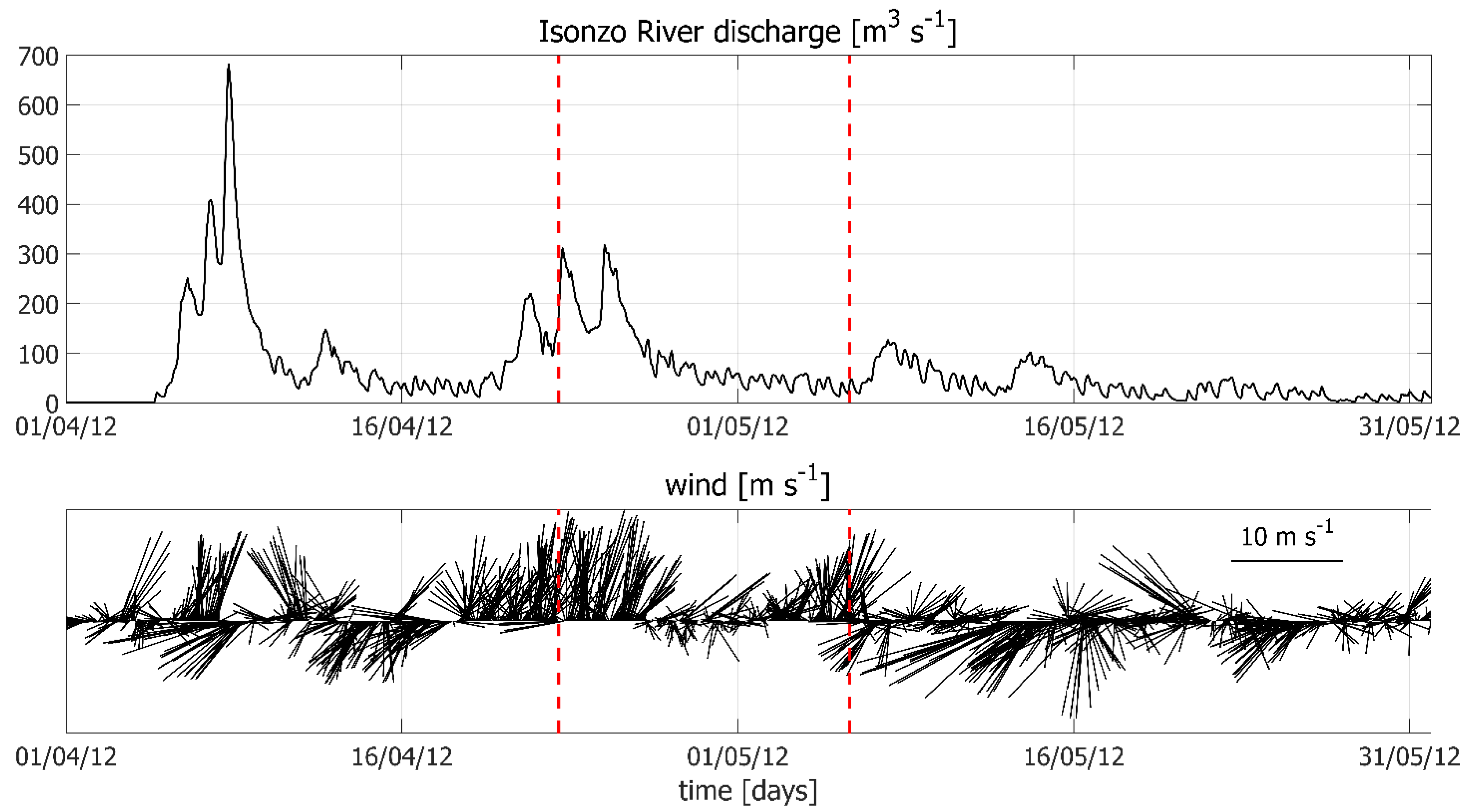
3.1. Description of the Meteo-Oceanographic Conditions during the TOSCA Experiment

The circulation in the GoT during the TOSCA experiment was strongly influenced by peculiar hydrological and meteorological conditions. A detailed look into the runoff and wind data is provided in Figure 2, which shows the Isonzo river discharge and the stick diagram of wind direction and speed during April and May 2012.

April was characterized by two significant flood events, with an exceptional freshwater discharge peaking up to 700 m³/s during the first episode (5–9 April) and a relatively long-lived event (20–26 April), which started 3 days before the beginning of the TOSCA drifter experiment.

On the contrary, during May, the Isonzo flow rate was quite low (almost always below 100 m³/s).

April was also characterized by significant southerly wind episodes, in particular during the second Isonzo flood. It must be pointed out that this is a typical meteo-hydrologic condition for the GoT and, in general, for the northern Adriatic Sea. Southerly winds accumulate moisture when blowing over the Ionian and eastern Mediterranean Seas; moreover, air humidity increases further along the path through the Adriatic Sea. These very humid air masses eventually reach the mainland and hit the Alpine arch, slowing down and discharging their water content through heavy rainfall over northern Italy. When blowing along the Adriatic Sea main axis, these winds also pile up water and favor storm surges in the northern sectors, thus blocking river discharge.

Conversely, May showed stronger meteorological variability, with intense easterly wind episodes (i.e., Bora) and land/sea breezes, which favor water mass renewal in the GoT.

The first TOSCA experiment was conducted between 23 April and 5 May 2012. Sequences of daily averaged HFR current maps during the experiment, overlapped with the daily drifter trajectories, are provided in Figure 3 and Figure 4. A couple of eddies (large-clockwise and smaller-counterclockwise, Figure 3) were already present in the GoT when the first drifters were deployed on 23 April. We hypothesize that those eddies were generated by the preconditioning event characterized by a quite intense (up to ~200 m³/s) freshwater discharge from the Isonzo river and dominant southerly winds (Figure 2). The same conditions were met during the following two days, when southerly winds were still predominant and freshwater discharge peaked two times, up to 300 m³/s. Persistent southerly wind blew also when the river discharge decreased significantly.

Drifters accurately tracked the observed HFR currents, identifying a clockwise, basin-wide general circulation pattern in the Gulf, with a strong daily variability that appears to be related mainly to the local wind (Figure 3 and Figure 4).

Drifter trajectories showed anticyclonic patterns almost everywhere. Large loops (diameter of about 12 km) prevailed in the center of the Gulf, especially at the beginning of the experiment and at the end of it. The areas closer to the coast were characterized by smaller loops, with diameters between 2 and 5 km throughout the experiment. During strong wind episodes, drifter paths were more elongated and did not form closed loops. Some inertial oscillations were also observed, although drifters mainly moved straight towards the coast.

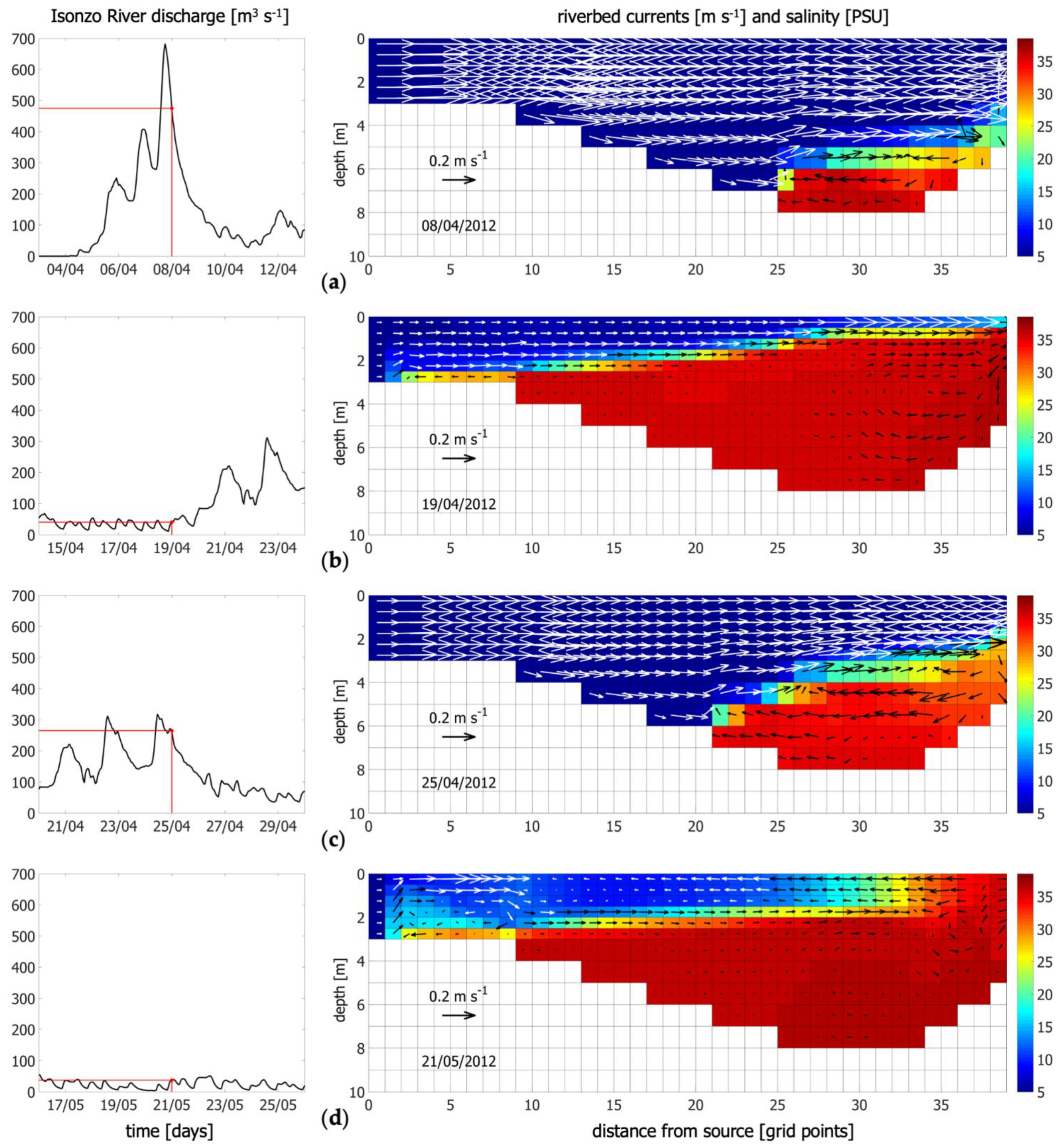
3.2. Modelling the Freshwater Input

When simulating ocean processes in ROFI areas, particular attention must be paid to correctly reproduce the freshwater input. In this section, we will show how the setting described in Section 2.1.1 can provide a realistic representation of the thermohaline and momentum contribution of the main river flowing into the GoT: the Isonzo/Soča river.

Four examples of the most significant hydrologic conditions that can be observed are reported in Figure 5. The panels on the right show the vertical section of the Isonzo riverbed, which was simulated as a one grid cell-wide channel (Figure 1c), with the depth obtained from in-situ samplings [5]. The values of temperature, salinity and barotropic velocity are imposed (as local open-boundary conditions) at the upstream limit of the channel (left side of the panels). The river mouth is located on the right side of the panels.

Figure 5a shows that only in the case of very strong floods (~700 m³/s), freshwater occupies almost the entire riverbed and the choice of imposing the prescribed velocity and salinity at the river mouth or a few kilometers upstream should not make a remarkable difference. In the case of low discharge (Figure 5b), if the freshwater source is far from the mouth, there is time and space for the salt wedge to develop. Low salinity water masses, originally imposed at the river spring and along the entire water column (i.e., open-boundary conditions applied to the model grid), tend to rise to the surface layers, with entrainment of seawater and consequent increase of salinity. During average flood conditions (Figure 5c), the situation is halfway between (a) and (b), with a balance between the freshwater outflow and the salt wedge inflow. In the case of both very low discharge rates and wind blowing from the mouth along the channel, the river plume could even go back upstream, with a consequent lack of freshwater at the river mouth (Figure 5d).

With these examples we want to highlight the importance of a realistic representation of freshwater discharge in high-resolution studies. Other approaches such as introducing a localized precipitation at the river mouth or imposing open-boundary conditions, without a long enough riverbed, could result in an unrealistic representation of the momentum contribution, in the first case, or an inaccurate estimation of river salinity and buoyancy, in the second.

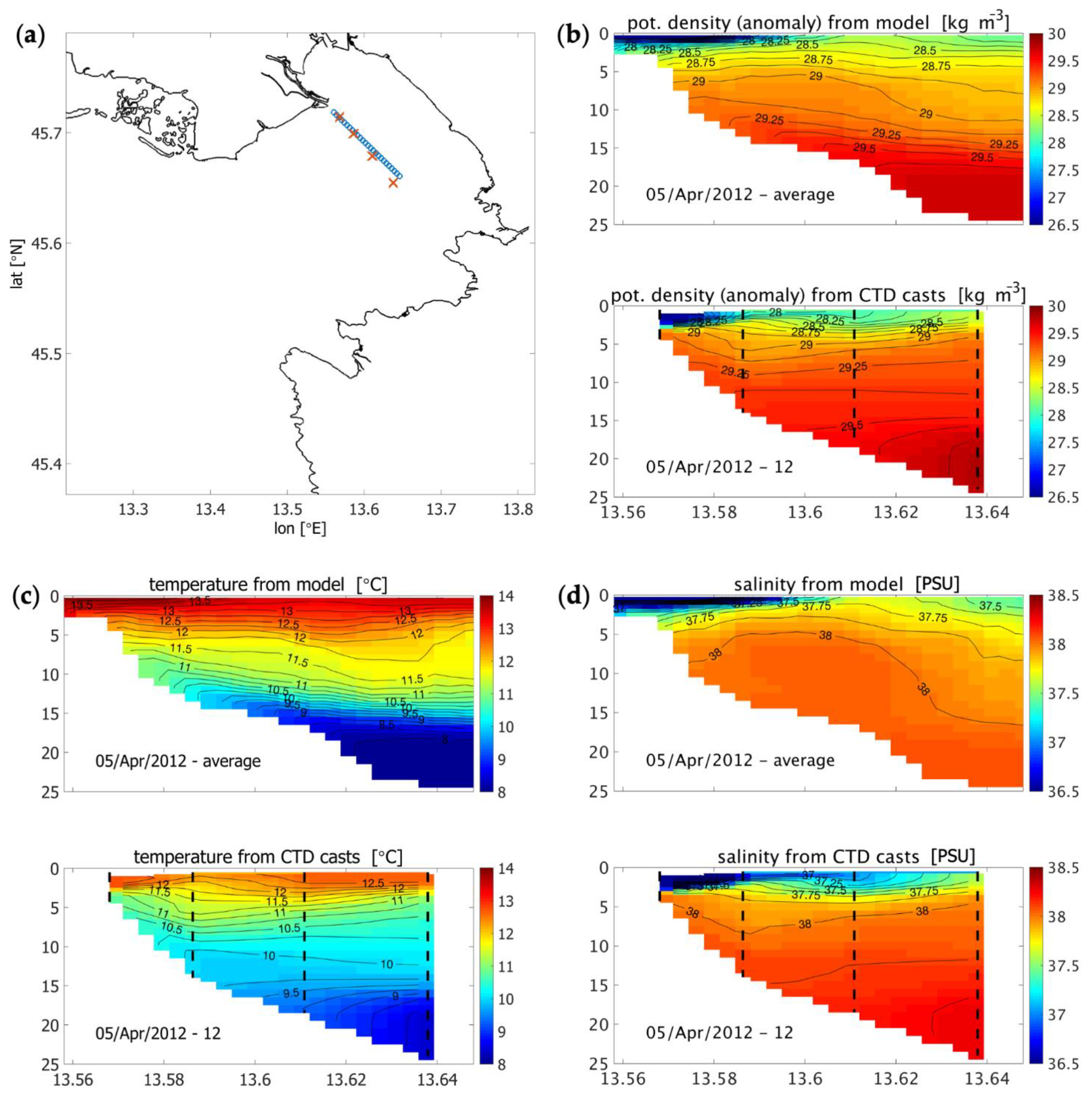
3.3. Comparison between Model Results and CTD Casts

A series of temperature and salinity casts were collected in the first week of April 2012 along a transect starting from the Isonzo river mouth (Figure 6a). Data from the casts were used as a validation of the model’s capability in reproducing the observed oceanographic conditions prior to the beginning of the TOSCA experiment. In general, the model seems to reconstruct the observed stratification in the potential density anomaly transect relatively well (Figure 6b), with a clear stratification pattern with light waters at the surface. However, Figure 6c shows that the model is warmer at the surface and colder at the bottom than what was observed from the CTD casts. Salinity data show a good match between the model and observations with respect to the thickness of the freshwater layer close to the river mouth (Figure 6d). Nevertheless, a portion of the modelled freshwater plume is displaced further away from the mouth, forming a lens of fresher water in the center of the domain, while CTD casts do not show this peculiarity. The model also underestimates salinity in the deeper layers. It is worth noting that daily averaged temperature, salinity and potential density fields from the model were used in this comparison.

3.4. Comparison between Model Results and HF Radar Data

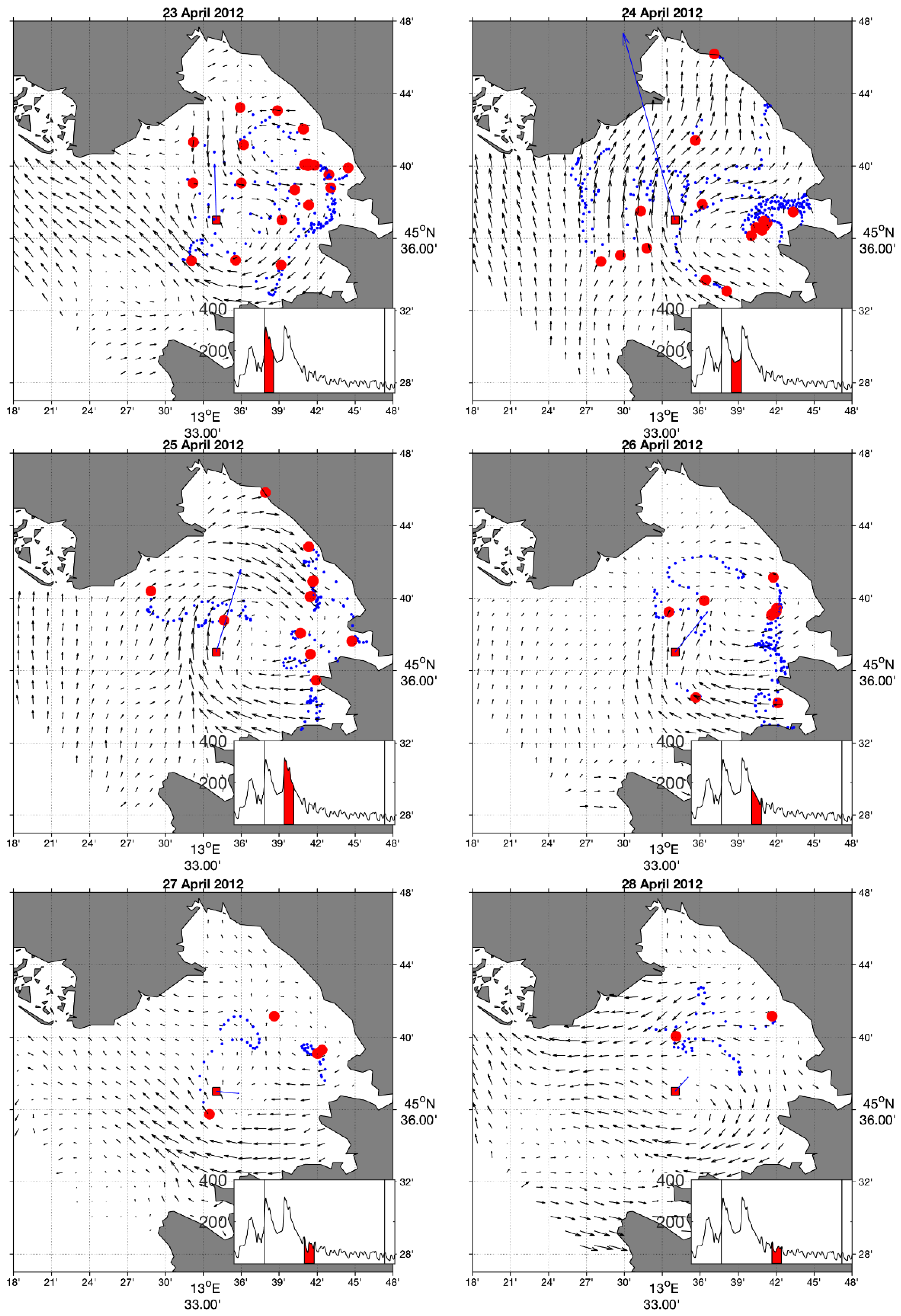
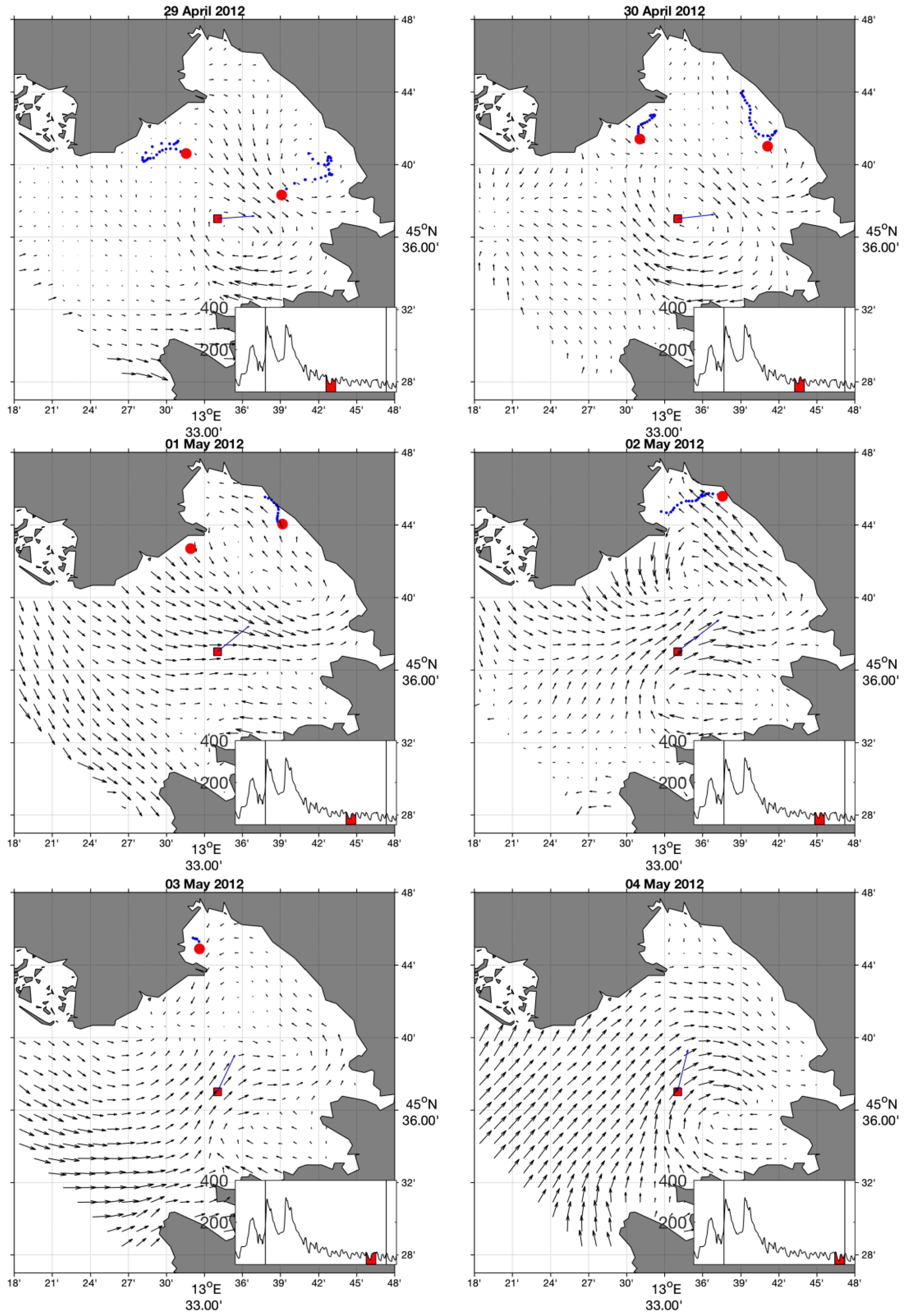
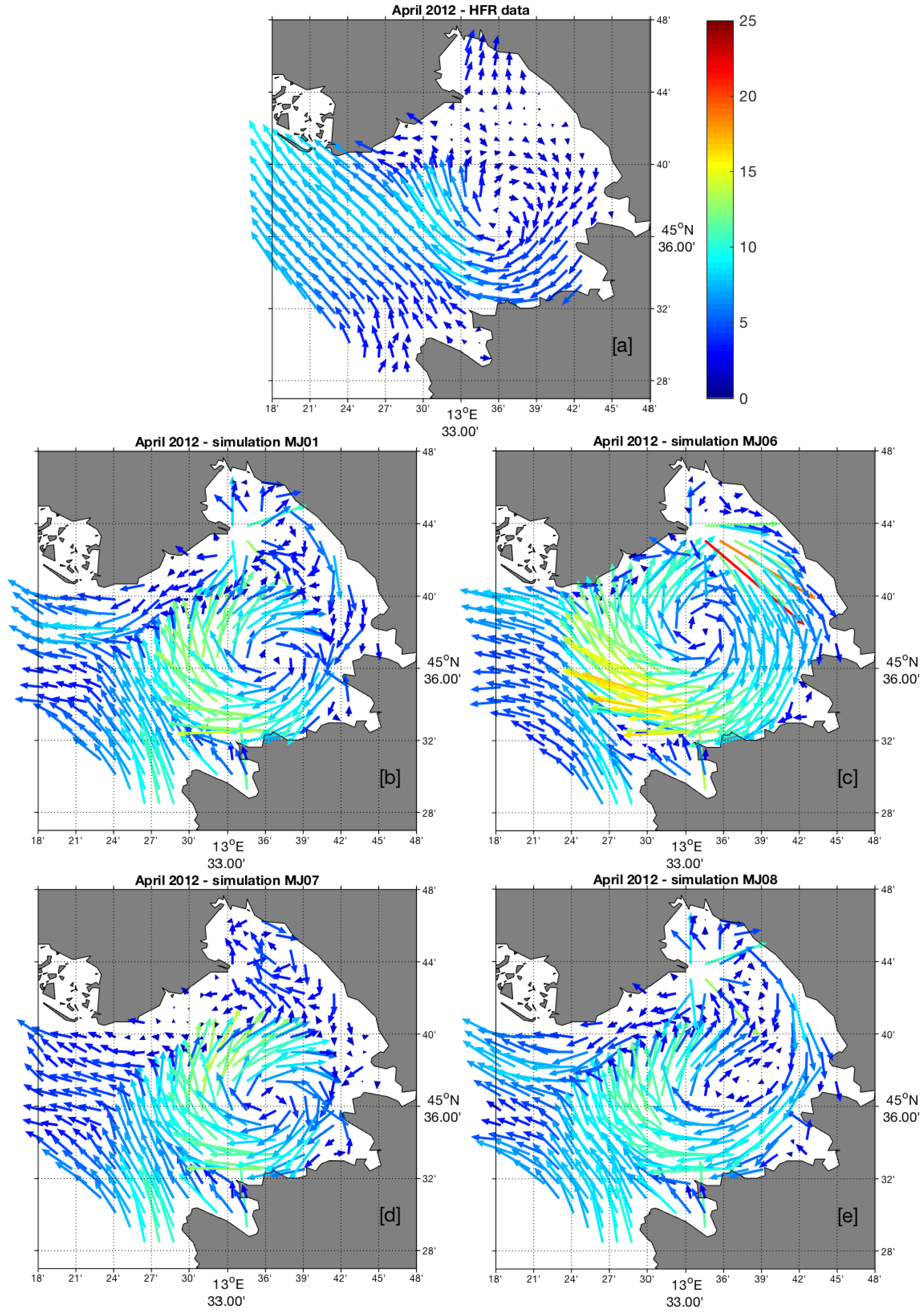
3.4.1. Surface Current Maps

Monthly averaged surface currents derived from the HFR measurements suggest the presence of a persistent clockwise-rotating structure in the central part of the GoT for both April and May 2012 (Figure 7a and Figure 8a, respectively), modulated by the different meteorological and hydrological forcing conditions (Figure 2). Weak currents characterize the northernmost part of the basin. A strong north-westward current can be observed during April 2012 at the entrance of the GoT, which is consistent with the typical circulation structure of the Adriatic Sea. On the opposite, average surface currents from HFR for May 2012 show a stronger outflow along the Italian coastline on the northernmost portion of the domain, enhanced by easterly wind episodes. Indeed, the wind stick diagram shown in Figure 2 spots (in May 2012) several episodes of northeasterly Bora wind, which is known to force water out of the GoT [6,7].

As detailed in Section 2.1.3, in order to understand and quantify the role of the different forcings acting on the basin, we analyzed the results of the simulation performed in the most interesting configurations, namely: full model setup (RR, Figure 7b and Figure 8b), simulation without wind forcing (NW, Figure 7c and Figure 8c), without river input (NR, Figure 7d and Figure 8d), and without tidal forcing (NT, Figure 7e and Figure 8e).

Model runs reproduced the average observed structures satisfactorily, both in April and May, with similar departures from HFR measurements. In particular, the model persistently shows a closed anticyclonic circulation at the surface (except in May, in the NW configuration, Figure 8c). This closed gyre is less evident in the HFR maps.

April is characterized by strong southerly winds and strong freshwater discharge, but the circulation seems to be mainly governed by the density structure. Switching off the freshwater and the tides does not change the circulation (Figure 7d,e), while the absence of wind enhances the anticyclonic gyre. In general, the model overestimates the current speed in the middle of the basin and lacks in reproducing the straight north-westward flow at the Gulf entrance. All simulations agree in generating the recirculation feature inside the Gulf, however its extent varies under the various model configurations. For instance, shutting wind forcing down (Figure 7c) removes the outflow along the northern coastline and enlarges the vortex structure, which occupies the entire GoT. Under this configuration, the absence of wind mixing and the strong freshwater input enhance the stratification, with an increased energy content in the surface layer. The effects of the freshwater discharge from the Isonzo river to the north are particularly clear, with current speeds exceeding 20 cm/s (on average).

On the other hand, the gyre is present even when the freshwater input in the GoT is shut down (Figure 7d), suggesting that the gyre depends on a combination of thermohaline stratification [6] and topographic (bathymetric) control, and might be also influenced by the inflow of fresher water from the Adriatic Sea, consistent with a hypothesis of remote forcing at the Adriatic basin scale [25].

In May, moderate Bora wind episodes occur and freshwater outflows are practically missing. Model runs reproduce the observed structures relatively well, including the recirculation feature inside the GoT, with the exception of the NW run (Figure 8c), where wind forcing was removed. In this case, the cyclonic structure vanishes and a different circulation pattern can be observed.

Nevertheless, the average current patterns obtained with the other model configurations (RR, NR, NT) are quite similar to HFR data, highlighting the importance of wind forcing in determining the circulation in May. Moreover, these simulations are only slightly affected by the prescribed different forcing conditions, in particular tides are not significant and the river contribution is very low, therefore, switching them on and off does not alter the monthly mean circulation pattern.

It must be also pointed out that HFR currents west from the line Piran—Grado seem less reliable in some areas and in specific periods: south of Grado in April (Figure 7a) and west of promontory Savudrija in May (Figure 8a). The difference between model and HFR measurements in these areas should be considered more carefully.

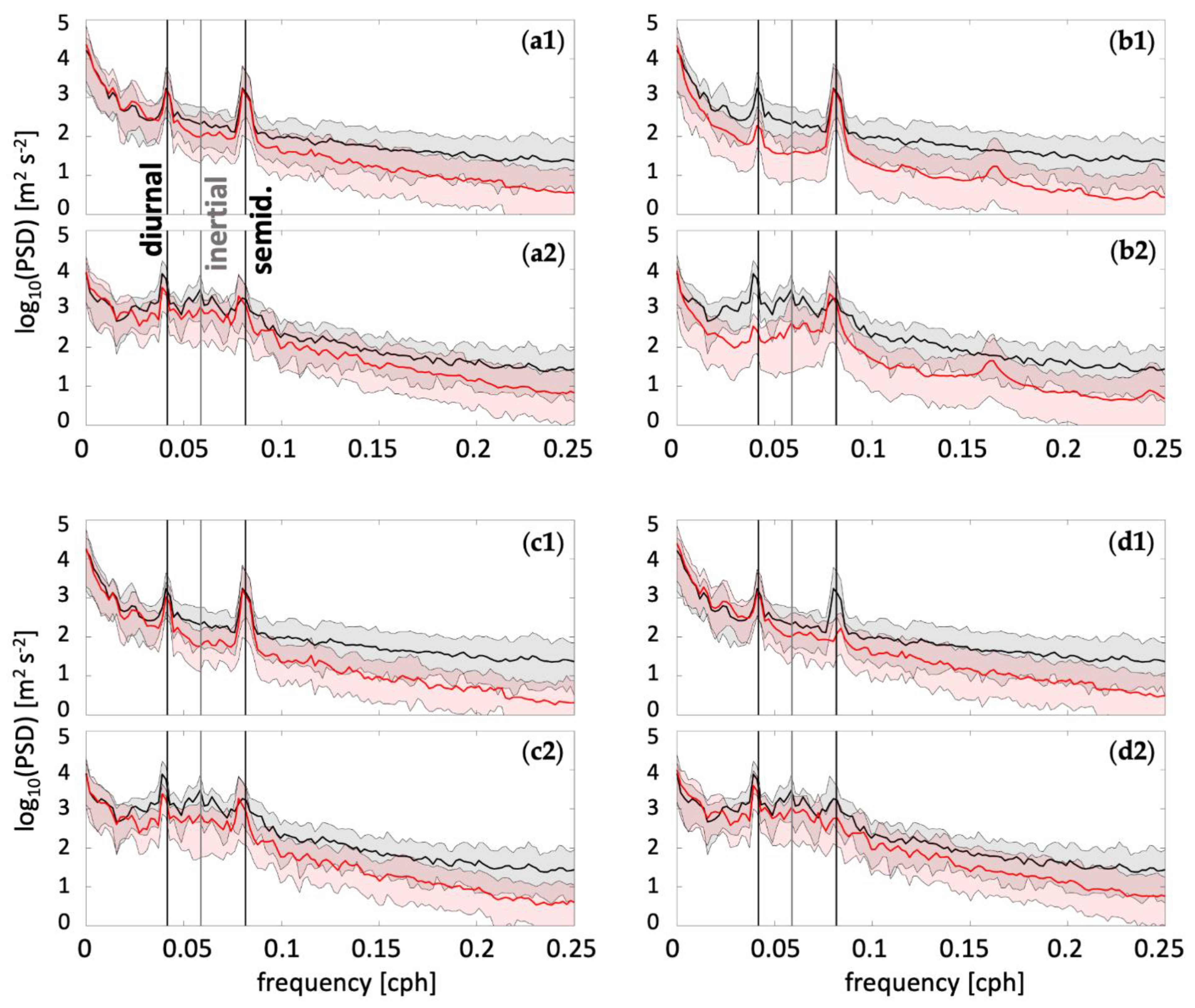
3.4.2. Power Spectral Density

A comparison in the distribution of model (HFR) variance over frequency for the April–May time period is provided in Figure 9. Rather than focusing on an individual grid cell, here we show results of the spatially averaged rotary spectra and use the 5–95th percentiles as a measure of the spatial homogeneity between HFR data and model simulations under different forcing conditions.

Common features in the HFR and simulated fields (Figure 9) include peaks at the semidiurnal frequency band (corresponding to the M₂, S₂ tidal harmonics) and at the diurnal frequency band (corresponding to the K₁ tidal constituent, but also an indication of wind-driven diurnal currents associated with the land–sea breeze regime), high energy content within the inertial band of the anticyclonic component (approximately 17 h at the local latitudes), and energetic low-frequency components.

The effects of the different configurations adopted in this work can be clearly seen in the energy distributions and in the impacts on specific frequency bands. For instance, the inertial- and near-inertial energy bands decrease when the model is run without wind forcing (scenario “b”) or, to a lesser extent, without freshwater input (scenario “c”), consistent with the impact of vertical stratification on the strength of the inertial motions. It should be noted, however, that, even in the full configuration mode, the model still seems to slightly underestimate energy levels in this band.

Shutting down the wind has also a clear effect on the energy in the diurnal band, which suggests that diurnal land–sea breeze is important in this time of the year, and in the subtidal, low-frequency portion of the spectra.

Removing tides from the model open boundary affects primarily the semidiurnal frequency band, with only a minor impact (in terms of model energy) within the diurnal frequency band. It is interesting to note the presence of higher frequency harmonics (the period of approximately 6–8 h) in the high-frequency tails of the model spectra that appear when wind is shut down, most likely due to the open-boundary conditions imposed to the model in this run.

3.5. Drifter (Real and Virtual) Data Analysis

As specified in Section 2.5.2, spatially sparse drifter currents were mapped onto the radar observational grid. Similarly (Section 2.5.1), model currents at the domain nodes closest to the HFR grid points were associated with the corresponding HFR grid location. To avoid introducing biases in the comparison metrics due to missing data in the HFR dataset, temporal gaps in the HFR dataset were propagated through the remapped model and drifter velocity data.

3.5.1. Radar–Drifter Comparison

The full set of drifters deployed in the GoT provided a statistically significant number of hourly observations of velocities (in excess of 700). Metrics for the HFR-drifter comparisons during the TOSCA experiment, summarized in

Table 2. Comparison metrics (scalar correlation coefficient R, slope and intercept of the linear best fit model) for the HFR-drifter data, separate for the U (V) velocity components, along with the 95% confidence levels (CL) and the number of samples (n) used in the comparisons.

	R (95%CL)	a (95%CL)	b (95%CL)	n
HFR-U	0.7561	0.6742	−0.4870	713
	(0.7228, 0.7859)	(0.6312, 0.7172)	(−1.1212, 0.1473)
HFR-V	0.7468	0.5951	1.9872	713
	(0.7124, 0.7775)	(0.5561, 0.6341)	(1.3691, 2.6052)

, provide typical correlation values for the U (V) components of R_U = 0.76 (R_V = 0.75), with slope and intercept values of the regression line a_U = 0.67 (a_V = 0.60 cm/s) and b_U = −0.48 (b_V = 1.99 cm/s), respectively. Comparison metrics for HFR observation within the GoT are consistent with, if not even better than, comparison metrics derived from drifters in other regions (see, for instance [48,49]).

3.5.2. Model–Drifter Comparison

In analogy with the HFR-drifter comparison,

Table 3. Comparison metrics (scalar correlation coefficient R, slope and intercept of the linear best fit model) for the model–drifter data, separate for the U (V) velocity components, along with the 95% confidence levels (CL) and the number of samples (n) used in the comparisons. Summary is provided for the model runs reported in Table 1.

	R (95%CL)	a (95%CL)	b (95%CL)	n
RR-U	0.313	0.2186	1.2134	713
	(0.2452, 0.3777)	(0.1698, 0.2675)	(0.4922, 1.9346)
RR-V	0.2406	0.164	0.726	713
	(0.1702, 0.3086)	(0.1153, 0.2128)	(−0.0457, 1.4977)
NW-U	0.3948	0.1918	1.9718	713
	(0.3309, 0.4550)	(0.1589, 0.2247)	(1.4866, 2.4570)
NW-V	0.3025	0.1373	−2.4317	713
	(0.2343, 0.3678)	(0.1054, 0.1691)	(−2.9360, −1.9274)
NR-U	0.3981	0.227	2.7082	713
	(0.3344, 0.4581)	(0.1885, 0.2655)	(2.1396, 3.2769)
NR-V	0.1876	0.0954	2.1136	713
	(0.1158, 0.2575)	(0.0586, 0.1322)	(1.5313, 2.6960)
NT-U	0.2982	0.2013	1.8935	713
	(0.2298, 0.3637)	(0.1539, 0.2488)	(1.1930, 2.5939)
NT-V	0.213	0.1416	2.2624	713
	(0.1418, 0.2821)	(0.0938, 0.1895)	(1.5050, 3.0198)

summarizes the results of the model–drifter comparison for all the different model runs considered in this paper (Table 1). It is clearly seen that regardless of the forcing used in the simulations, each model run underperforms relative to the HFR data in reconstructing the near surface velocities derived from drifter observations. For the U (V) components, scalar correlation is in the range R_U = (0.30, 0.40) (R_V = (0.19, 0.30)). Typical values for the slopes and intercepts of the linear regression model are in the range a_U = (0.19, 0.23), b_U = (1.21, 2.71) cm/s, and a_V = (0.10, 0.16), b_V = (−2.43, 2.26) cm/s, for the U and V components, respectively.

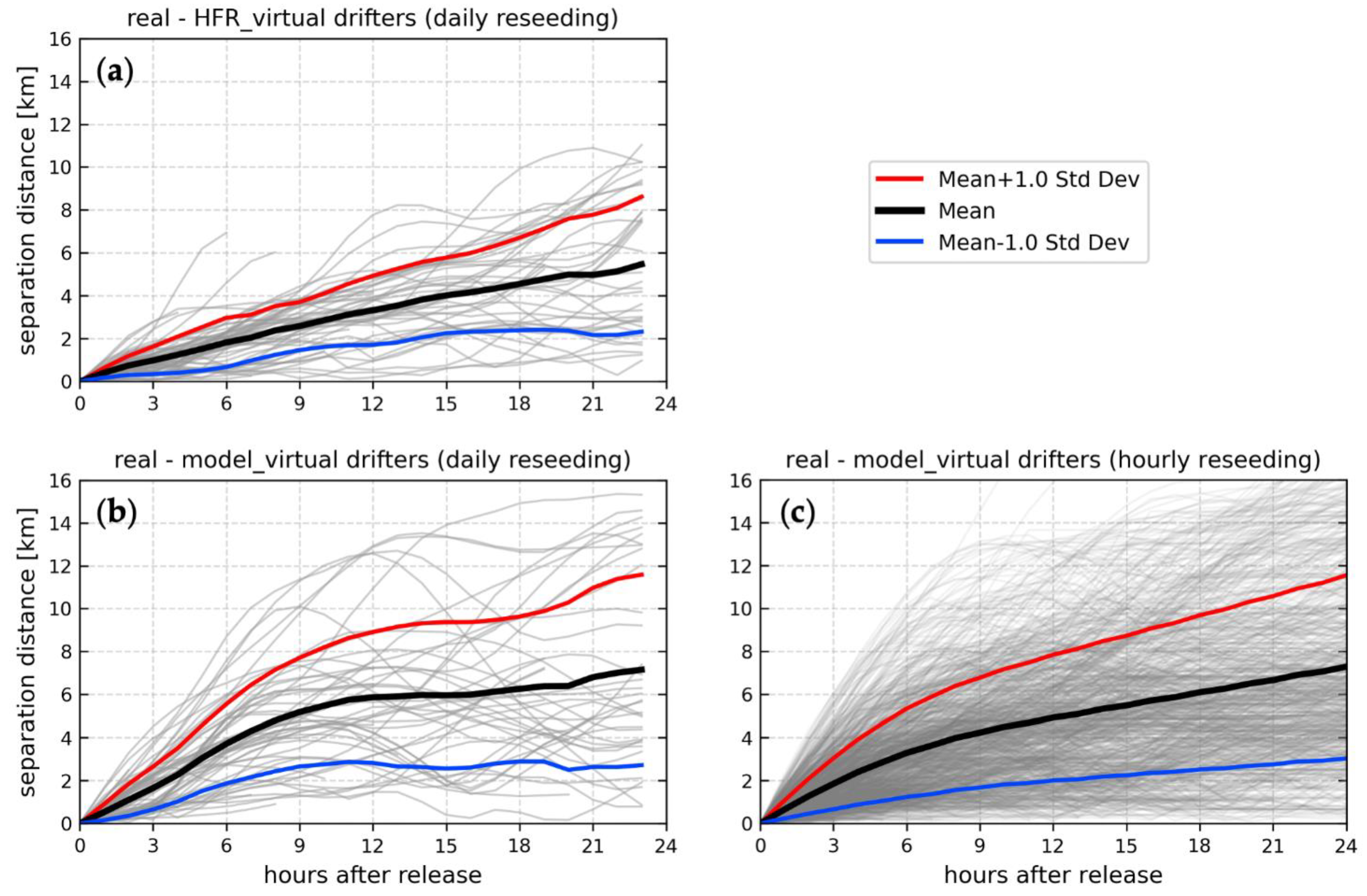
3.5.3. Separation Distance between Real and Virtual Drifters

Real drifter (RD) trajectories were compared against both virtual trajectories derived from model results (henceforth, VDM) in the full configuration (RR) and virtual drifters computed from HFR velocity fields (VDR). In order to test model sensitivity to the reseeding time interval, we also computed the separation distances, considering both daily and hourly reseeding of the virtual drifters on the model velocity fields (i.e., every virtual drifter was redeployed on the corresponding real drifter position every day or every hour).

For every drifter $n$, the separation distances between the real and virtual drifter of coordinates $\left(X_n^{RD}\left(t\right),Y_n^{RD}\left(t\right)\right)$ and $\left(X_n^{VD}\left(t\right),Y_n^{VD}\left(t\right)\right)$ are computed as

$$S{D}_n\left(t\right)=\sqrt{{\left(X_n^{RD}\left(t\right)-X_n^{VD}\left(t\right)\right)}^2+{\left(Y_n^{RD}\left(t\right)-Y_n^{VD}\left(t\right)\right)}^2}$$

(3)

and are presented in Figure 10. As specified in the previous section (and also as reported in [3]), the mean separation distance between RD and VDR reaches less than 6 km in 23 h. The comparison between RD and VDM gives slightly worse results (slightly more than 7 km) when considering both hourly or daily reseeding of the virtual drifters. Indeed, the use of hourly reseeding (Figure 10c) does not change the mean separation distance reached after 24 h. The analysis with hourly reseeding includes 1095 trajectories (and separation distances) lasting between 1 and 24 h, much more numerous than the trajectories inspected by using daily reseeding, which are only 67.

The analysis of the mean absolute distance performed by Bellomo et al. [3] showed that the drifter travel distance reaches a plateau (~5 km) after 12 h, suggesting that the size of the domain (i.e., boundary effects) and the re-circulations induced by eddies and flow variability become dominant after that time. In other words, during the first TOSCA experiment the peculiar circulation features, with several eddies and re-circulations, moved (on average) the drifters back towards the areas of initial deployment, limiting the increase of the travel distance.

The separation distance RD-VDR increases linearly in time (Figure 10a): it is less than 2 km after 6 h from deployment, less than 4 km after 12 h and less than 6 km after 24 h from deployment. Instead, the separation distance RD-VDM evolves similarly to the travel distance (Figure 10b), increasing faster at the beginning and with a lower rate after 12 h. This means that the initial separation rate of the trajectories is too high and the model results are not able to realistically reproduce the observed trajectories. The application of hourly reseeding (Figure 10c) gives better results within the recirculation time period (12 h), with a lower initial increase rate than the daily reseeding case, followed by an almost linear trend. Such a slight improvement could be also due to the fact that more tracks imply more robust statistics.

We also tested the separation distance RD-VDM using the other test cases of Table 1 (NW, NR, NT) and changing the initial deployment of the virtual drifters (+/− 1 h, +/− 12 h), obtaining very similar results (not shown). This means that the circulation patterns are so complex, with strong space–time variability, that our model, despite the accuracy of the setup and forcing, on average, was not able to track efficiently the RD trajectories in those particular environmental conditions.

In order to investigate the possible origin of the divergence of modelled trajectories, hydrodynamic/meteorological features, such as currents, wind intensity, seawater temperature and salinity, as well as local features, such as depth and distance from the coast, were extracted along the path of the VDM. The Pearson product–moment correlation coefficients between the hourly values of each of these properties, and the hourly increase in separation distance of the single drifters, are presented in Figure 11, together with the associated p-value indicating the significance of the correlation coefficients. It appears that the distance from the coast and the current intensity can be associated with the hourly increase in the separation distance until the 16th hour, after which the p-value indicates that the correlation coefficients are no longer statistically significant (p-value > 5%). To a smaller extent, wind intensity and temperature suggest being very slightly correlated (with positive and negative correlations, respectively) up to the fourth hour. Salinity and local depth, instead, show that possible linear relationships with the separation distance are not present, or that they are poor.

To better visualize and understand how the shape of the domain and, more specifically, the distance from the coast influences the separation distance, Figure 12 presents a map of the GoT where the positions of the VDM drifters (hourly release) are represented by dots, the color of which is proportional to the (hourly) increase of the separation distance. As expected, most of the lowest increases in the separation distance are found close to the coast, and they are even smaller next to the most confined coastal areas. The comparison with the maps of the average current intensity in Figure 7 and Figure 8 show that currents, as expected, tend to be weaker next to small and shallow embayments (due to bottom friction and bathymetric constraints). This might also be at least partially responsible for the correlation observed between the separation distance and the current intensity. Another area with small separation distances is the northern coastal strip, west of the Isonzo river mouth. In that area, during the observed time period velocities were small and, most important, aligned with the coastline. Such a topographic constraint could reduce drifter divergence, enhancing VDM drifter reliability. Conversely, the internal area of the Gulf shows much higher separation distances, with some exceptions in the middle of the basin where the increase in the separation can be relatively low.

4. Discussion and Conclusions

The paper presents a detailed analysis of the circulation pattern that was observed in the GoT during the April–May 2012 TOSCA experiment, when intense freshwater inflow and strong southerly winds characterized the region. A unique dataset, comprising HFR and drifter observations, was used in combination with model simulations to try to understand the complex driving mechanisms in the GoT.

High-resolution numerical simulations were compared to surface currents obtained from HF radar measurements and drifter data. To date, this is the first experimental data set in the area having a similar resolution in time and space, and it can be considered a sort of “natural” integration of HF radar measurements performed in the surrounding area in the past 10 years [9,10].

HFR observations have been extensively validated against moored or vessel-mounted current meters over a wide variety of environments. The direct comparisons against the drifter dataset deployed during the TOSCA experiment further prove their overall reliability, with high correlation values (typically above 0.74 for both the scalar velocity components) and low biases. Comparison metrics are consistent with, if not better than, similar validations against drifters elsewhere. HFR suggested the presence of a persistent gyre that could be observed in the monthly averaged surface current maps. Drifter data collected within the GoT confirmed the presence of this feature in the Gulf.

Nevertheless, particular care must be taken when considering surface velocity fields in the shallowest areas of the basin, where HFR systems can be less accurate. Indeed, at the 25 MHz operating frequency, Bragg-matching ocean waves have a wavelength of approximately 6 m. The water depth at which the deep-water approximation for the first order return is no longer valid (ZL) is given by

$$ZL=\frac{Z}{L}<1$$

(4)

where Z is the water depth and L the dominant wavelength. At 25 MHz, this condition is met where the bathymetry is shallower than 6 m: in the GoT, along the northernmost coastal areas of the basin and close to the Isonzo/Soča river mouth (Figure 1c). These areas represent only a minor portion of the domain; therefore, they are of little importance to the overall comparison between radar and drifters, also considering that very few drifters were found there during the experiment. However, a direct comparison between HFR and model-derived surface velocity maps can be less reliable along that coastal strip.

Low salinity (hence, low conductivity) water masses can attenuate the signal to noise ratio of the Bragg echo [50], thus possibly increasing the error in retrieving HFR currents in the shallow northern area, close to the river mouth, where salinity can drop to very low values.

Model configuration features high resolution in space (~250 × 350 m) and time (hourly averaged output) and takes into account all the major forcings acting on the basin (wind, heat fluxes, river discharge, tides, northern Adriatic circulation). The model is coupled at an hourly frequency with a 4.4 km resolution state-of-the-art atmospheric model, run in hindcast mode. The Isonzo/Soča river runoff was simulated by taking into account a realistic shape of the riverbed, thus allowing for the formation of thin surface freshwater layers and salt wedges, modulated by tides, or strong vertically uniform outflows during major flood events. In general, the model reproduced correctly the initial thermohaline stratification (Section 3.3), the (monthly) mean observed surface circulation features (Section 3.4.1) and the energy distribution at the various frequencies (Section 3.4.2) but, despite the care in setting up the system, failed at tracking the observed drifter trajectories, especially in the internal part of the Gulf, while better accuracy was observed next to the coast. This can be due to inaccuracies in model setup and forcing, but it can be also ascribed to the complexity of the circulation patterns during the TOSCA experiment, with intense freshwater floods, strong wind variability, fronts and re-circulations [3]. In such a context, errors in the initial phase of the simulated inertial currents can lead to significant divergence between the real and virtual (model) trajectories. Moreover, spectral analysis (Figure 9) has shown that the model underestimates the inertial motions, further contributing to the separation between real and simulated drifter paths.

It must be pointed out that, among the five sites investigated in the TOSCA project, the GoT showed the lowest value (1.6) of the search range reduction factor (SRRF [3]), also proving that VDR, which are based on measured HFR data, cannot efficiently track the observed drifter trajectories. This can be due to the HFR data gaps and the relatively coarse resolution of the HFR velocity fields that do not allow for a detailed description of small-scale dynamics. Indeed, even if the comparison of the scalar components of the Eulerian gridded velocity fields gives good results (Section 3.5.1), there is less confidence in the comparison of the Lagrangian drifter trajectories because no HFR or model gridded fields can fully reproduce the observed variability of the (real) Lagrangian paths. For example, gridded velocity fields cannot take into account small-scale processes such as velocity shear (horizontal in HF radar data; horizontal and vertical in the model) or sub-grid-scale turbulence.

Regarding the capability of forecasting the position of surface objects for SAR applications, the present model configuration is not able to predict the correct position under similar environmental conditions, which are too complex to be accurately reproduced. It must be also pointed out that the model neglects surface waves, and Stokes’ drift has an important role in transporting a floating body [51]. Furthermore, the model also cannot solve important turbulent processes driven by wind and surface waves such as Langmuir circulations [52,53]. Finally, in this study we used CODE drifters, which are (although poorly) influenced by the wind. Undrogued CODE drifters have a general downwind slippage of about 1% of the wind speed due to Ekman currents, surface waves (e.g., Stokes’ drift) and direct exposure to wind of the emerging elements of the drifters (mostly the antenna) [54]. The actual model implementation does not allow to simulate these processes.

On average, the general surface circulation showed a stable anticyclonic pattern which lasted for two months (April and May). Previous studies already hypothesized the presence of alternating cyclonic-anticyclonic flow in the surface layer of the GoT, modulated by the diurnal sea breezes or by westerly-easterly winds. Moreover, tidal contributions were shown to be important only under calm weather conditions [14,21]. In our study, tides also do not affect the circulation (on a monthly timescale).

The possibility of an anticyclonic recirculation pattern in the GoT has already been documented through numerical simulations. Zavatarelli and Pinardi [25] evidenced this pattern during the stratified season (summer) by using both the 5-km resolution Adriatic Intermediate Model (AIM; [24]) and the high-resolution (1.5 km) Northern Adriatic Shelf Model (NASM; [25]). Similarly, using the Princeton Ocean Model (POM), Malacic and Petelin [6] showed that an anticyclonic circulation develops in the surface (down to 8 m depth) of the Gulf during the strongly stratified season, mostly due to the increased freshwater input of the Isonzo/Soča river.

In this study, we confirm the previous findings, highlighting the role of the different forcings acting on the basin. During April, model results show a general clockwise circulation in all the four main configurations (reference run (RR), no wind (NW), no river (NR), no tides (NT), Figure 7), meaning that all the forcing factors modulate the surface velocity regime, but the overall circulation structure is driven by the basin-wide Adriatic circulation and by the internal thermohaline properties of the basin (i.e., bowl-like vertical profile of density in the upper part of the water column [6], Figure 13). Conversely, in May, when the freshwater discharge is reduced, the circulation is significantly affected by the wind. Figure 8 clearly shows that only the NW run fails to reproduce the observed anticyclonic pattern (Figure 8c).

Figure 13 highlights the typical anticyclonic circulation pattern, with a dome-like structure of the sea surface height and a bowl-like density profile. In April, the large amount of freshwater discharged by the Isonzo/Soča river and the strong southerly wind regime induce a remarkable south–north-sea level gradient, with water masses piled up against the northern coast of the GoT. In May, low discharge rates and Bora wind episodes reduce the sea level gradient and maintain the anticyclonic density structure. Compared to the general average picture of the (cyclonic) circulation in the subsurface layers of the GoT, April and May 2012 represent a relatively long-lived anomalous condition, with a permanent anticyclonic gyre.

Despite being limited to the surface layer, the good results of the comparisons suggest that, in general, the model reconstructs the observed basin-scale dynamics. However, further tests and sensitivity analyses are required to fully calibrate the system for operational purposes. Among the possible improvements, we mention the increase of the resolution of both the oceanographic and the atmospheric model, a fine tuning of the turbulence parameterization, and the integration of a surface wave module and near-real-time data assimilation algorithms. The joint use of finite-time and finite-size Lyapunov exponents (FTLEs and FSLEs) and Lagrangian Coherent Structures (LCSs) could also improve the reliability of operational tools for SAR applications, with respect to the ones based uniquely on the tracking of single numerical trajectories [55].

All these aspects are being considered in view of an integrated operational platform for monitoring and forecasting the oceanographic conditions of the GoT.

References

1. Roarty, H.; Cook, T.; Hazard, L.; George, D.; Harlan, J.; Cosoli, S.; Wyatt, L.; Alvarez Fanjul, E.; Terrill, E.; Otero, M.; et al. The Global High Frequency Radar Network. Front. Mar. Sci. 2019, 6, 164. [Google Scholar] [CrossRef]
2. Testor, P.; de Young, B.; Rudnick, D.L.; Glenn, S.; Hayes, D.; Lee, C.M.; Pattiaratchi, C.; Hill, K.; Heslop, E.; Turpin, V.; et al. OceanGliders: A Component of the Integrated GOOS. Front. Mar. Sci. 2019, 6, 422. [Google Scholar] [CrossRef] [Green Version]
3. Bellomo, L.; Griffa, A.; Cosoli, S.; Falco, P.; Gerin, R.; Iermano, I.; Kalampokis, A.; Kokkini, Z.; Lana, A.; Magaldi, M.G.; et al. Toward an Integrated HF Radar Network in the Mediterranean Sea to Improve Search and Rescue and Oil Spill Response: The TOSCA Project Experience. J. Oper. Oceanogr. 2015, 8, 95–107. [Google Scholar] [CrossRef]
4. Simpson, J.H. Physical Processes in the ROFI Regime. J. Mar. Syst. 1997, 12, 3–15. [Google Scholar] [CrossRef]
5. Covelli, S.; Piani, R.; Faganeli, J.; Brambati, A. Circulation and Suspended Matter Distribution in a Microtidal Deltaic System: The Isonzo River Mouth (Northern Adriatic Sea). J. Coast. Res. 2004, 41, 130–140. [Google Scholar]
6. Malačič, V.; Petelin, B. Climatic Circulation in the Gulf of Trieste (Northern Adriatic). J. Geophys. Res. 2009, 114, C07002. [Google Scholar] [CrossRef]
7. Querin, S.; Crise, A.; Deponte, D.; Solidoro, C. Numerical Study of the Role of Wind Forcing and Freshwater Buoyancy Input on the Circulation in a Shallow Embayment (Gulf of Trieste, Northern Adriatic Sea). J. Geophys. Res. 2007, 112, C03S16. [Google Scholar] [CrossRef]
8. Chavanne, C.; Janeković, I.; Flament, P.; Poulain, P.-M.; Kuzmić, M.; Gurgel, K.-W. Tidal Currents in the Northwestern Adriatic: High-Frequency Radio Observations and Numerical Model Predictions. J. Geophys. Res. 2007, 112, C03S21. [Google Scholar] [CrossRef] [Green Version]
9. Kovačević, V.; Gačić, M.; Mancero Mosquera, I.; Mazzoldi, A.; Marinetti, S. HF Radar Observations in the Northern Adriatic: Surface Current Field in Front of the Venetian Lagoon. J. Mar. Syst. 2004, 51, 95–122. [Google Scholar] [CrossRef]
10. Cosoli, S.; Gačić, M.; Mazzoldi, A. Surface Current Variability and Wind Influence in the Northeastern Adriatic Sea as Observed from High-Frequency (HF) Radar Measurements. Cont. Shelf Res. 2012, 33, 1–13. [Google Scholar] [CrossRef]
11. Poulain, P.-M. Tidal Currents in the Adriatic as Measured by Surface Drifters. J. Geophys. Res. Oceans 2013, 118, 1434–1444. [Google Scholar] [CrossRef]
12. Stravisi, F. The IT Method for the Harmonic Tidal Prediction. Boll. Oceanol. Teor. Ed. Appl. 1983, 1, 193–204. [Google Scholar]
13. Cushman-Roisin, B.; Naimie, C.E. A 3D Finite-Element Model of the Adriatic Tides. J. Mar. Syst. 2002, 37, 279–297. [Google Scholar] [CrossRef]
14. Malačič, V.; Viezzoli, D. Tides in the Northern Adriatic Sea—The Gulf of Trieste. Nuovo Cimento 2000, 23, 365–382. [Google Scholar]
15. Dorman, C.E.; Carniel, S.; Cavaleri, L.; Sclavo, M.; Chiggiato, J.; Doyle, J.; Haack, T.; Pullen, J.; Grbec, B.; Vilibić, I.; et al. February 2003 Marine Atmospheric Conditions and the Bora over the Northern Adriatic. J. Geophys. Res. 2007, 112, C03S03. [Google Scholar] [CrossRef] [Green Version]
16. Raicich, F.; Malačič, V.; Celio, M.; Giaiotti, D.; Cantoni, C.; Colucci, R.R.; Čermelj, B.; Pucillo, A. Extreme Air-Sea Interactions in the Gulf of Trieste (North Adriatic) during the Strong Bora Event in Winter 2012. J. Geophys. Res. Oceans 2013, 118, 5238–5250. [Google Scholar] [CrossRef]
17. Querin, S.; Cossarini, G.; Solidoro, C. Simulating the Formation and Fate of Dense Water in a Midlatitude Marginal Sea during Normal and Warm Winter Conditions. J. Geophys. Res. Oceans 2013, 118, 885–900. [Google Scholar] [CrossRef]
18. Querin, S.; Bensi, M.; Cardin, V.; Solidoro, C.; Bacer, S.; Mariotti, L.; Stel, F.; Malačič, V. Saw-tooth Modulation of the Deep-water Thermohaline Properties in the Southern Adriatic Sea. J. Geophys. Res. Oceans 2016, 121, 4585–4600. [Google Scholar] [CrossRef] [Green Version]
19. Vilibić, I.; Mihanović, H.; Janeković, I.; Šepić, J. Modelling the Formation of Dense Water in the Northern Adriatic: Sensitivity Studies. Ocean Model. 2016, 101, 17–29. [Google Scholar] [CrossRef]
20. Janeković, I.; Mihanović, H.; Vilibić, I.; Tudor, M. Extreme Cooling and Dense Water Formation Estimates in Open and Coastal Regions of the Adriatic Sea during the Winter of 2012. J. Geophys. Res. Oceans 2014, 119, 3200–3218. [Google Scholar] [CrossRef]
21. Stravisi, F. Some Characteristics of the Circulation in the Gulf of Trieste. Thalass. Jugosl. 1983, 19, 355–363. [Google Scholar]
22. Cosoli, S.; Ličer, M.; Vodopivec, M.; Malačič, V. Surface Circulation in the Gulf of Trieste (Northern Adriatic Sea) from Radar, Model, and ADCP Comparisons: Hf Radar and Model Study of Trieste Gulf. J. Geophys. Res. Oceans 2013, 118, 6183–6200. [Google Scholar] [CrossRef]
23. Bogunović, B.; Malačič, V. Circulation in the Gulf of Trieste: Measurements and Model Results. Nuovo Cimento C 2009, 31, 301–326. [Google Scholar] [CrossRef]
24. Zavatarelli, M.; Pinardi, N.; Kourafalou, V.H.; Maggiore, A. Diagnostic and Prognostic Model Studies of the Adriatic Sea General Circulation: Seasonal Variability. J. Geophys. Res. 2002, 107, 3004. [Google Scholar] [CrossRef] [Green Version]
25. Zavatarelli, M.; Pinardi, N. The Adriatic Sea Modelling System: A Nested Approach. Ann. Geophys. 2003, 21, 345–364. [Google Scholar] [CrossRef]
26. Malačič, V.; Petelin, B.; Vodopivec, M. Topographic Control of Wind-Driven Circulation in the Northern Adriatic. J. Geophys. Res. Oceans 2012, 117, C06032. [Google Scholar] [CrossRef]
27. Marshall, J.; Adcroft, A.; Hill, C.; Perelman, L.; Heisey, C. A Finite-Volume, Incompressible Navier Stokes Model for Studies of the Ocean on Parallel Computers. J. Geophys. Res. Oceans 1997, 102, 5753–5766. [Google Scholar] [CrossRef] [Green Version]
28. Leith, C.E. Large Eddy Simulation of Complex Engineering and Geophysical Flows. Phys. Fluids 1968, 10, 1409–1416. [Google Scholar] [CrossRef]
29. Smagorinsky, J. Large Eddy Simulation of Complex Engineering and Geophysical Flows. In Evolution of Physical Oceanography; Orszag, S.A., Galperin, B., Eds.; Cambridge University Press: Cambridge, UK, 1993; pp. 3–36. [Google Scholar]
30. Large, W.G.; McWilliams, J.C.; Doney, S.C. Oceanic Vertical Mixing: A Review and a Model with a Nonlocal Boundary Layer Parameterization. Rev. Geophys. 1994, 32, 363–403. [Google Scholar] [CrossRef] [Green Version]
31. Campin, J.-M.; Heimbach, P.; Losch, M.; Forget, G.; Hill, E.; Adcroft, A.; Molod, A.; Menemenlis, D.; Ferreira, D.; Hill, C.; et al. MITgcm/MITgcm: Mid 2020 Version; Zenodo: Geneva, Switzerland, 2020. [Google Scholar]
32. Silvestri, C.; Bruschi, A.; Calace, N.; Cossarini, G.; Angelis, R.D.; Di Biagio, V.; Giua, N.; Saccomandi, F.; Peleggi, M.; Querin, S.; et al. CADEAU Project—Final Report, figshare, Iasi, Romania. 2020; 4399279. [CrossRef]
33. Erofeeva, S.; Padman, L.; Howard, S.L. Tide Model Driver (TMD) Version 2.5, Toolbox for Matlab; Earth & Space Research: Seattle, WA, USA, 2019. [Google Scholar]
34. Termonia, P.; Fischer, C.; Bazile, E.; Bouyssel, F.; Brožková, R.; Bénard, P.; Bochenek, B.; Degrauwe, D.; Derková, M.; El Khatib, R.; et al. The ALADIN System and Its Canonical Model Configurations AROME CY41T1 and ALARO CY40T1. Geosci. Model Dev. 2018, 11, 257–281. [Google Scholar] [CrossRef] [Green Version]
35. Strajnar, B.; Cedilnik, J.; Fettich, A.; Ličer, M.; Pristov, N.; Smerkol, P.; Jerman, J. Impact of Two-Way Coupling and Sea-Surface Temperature on Precipitation Forecasts in Regional Atmosphere and Ocean Models. Q. J. R. Meteorol. Soc. 2019, 145, 228–242. [Google Scholar] [CrossRef] [Green Version]
36. Fischer, C.; Montmerle, T.; Berre, L.; Auger, L.; Ştefănescu, S.E. An Overview of the Variational Assimilation in the ALADIN/France Numerical Weather-Prediction System. Q. J. R. Meteorol. Soc. 2005, 131, 3477–3492. [Google Scholar] [CrossRef]
37. Giard, D.; Bazile, E. Implementation of a New Assimilation Scheme for Soil and Surface Variables in a Global NWP Model. Mon. Weather Rev. 2000, 128, 19. [Google Scholar] [CrossRef]
38. Donlon, C.J.; Martin, M.; Stark, J.; Roberts-Jones, J.; Fiedler, E.; Wimmer, W. The Operational Sea Surface Temperature and Sea Ice Analysis (OSTIA) System. Remote Sens. Environ. 2012, 116, 140–158. [Google Scholar] [CrossRef]
39. Paduan, J.D.; Graber, H.C. Introduction to High-Frequency Radar: Reality and Myth. Oceanography 1997, 10, 36–39. [Google Scholar] [CrossRef]
40. Stewart, R.H.; Joy, J.W. HF Radio Measurements of Surface Currents. Deep Sea Res. Oceanogr. Abstr. 1974, 21, 1039–1049. [Google Scholar] [CrossRef]
41. Gurgel, K.-; Essen, H.-; Schirmer, F. CODAR in Germany–A Status Report Valid November 1985. IEEE J. Ocean. Eng. 1986, 11, 251–257. [Google Scholar] [CrossRef]
42. Gerin, R.; Poulain, P.-M.; Bussani, A.; Brunetti, F.; Zervakis, V.; Kokkini, Z.; Malačič, V.; Čermelj, B. First TOSCA Drifter Experiment in the Gulf of Trieste (April 2012); Technical Report 2012/91 OCE 6 SIRE; OGS: Trieste, Italy, 2012; p. 32. [Google Scholar]
43. Gerin, R.; Bussani, A. Nuova Procedura Di Editing Automatico Dei Dati Drifter Impiegata Su Oceano per MyOcean e Prodotti Web in Near-Real Time e Delay Mode; Technical Report 2011/55 OGA 20 SIRE; OGS: Trieste, Italy, 2011; p. 13. [Google Scholar]
44. Hansen, D.V.; Poulain, P.-M. Quality Control and Interpolations of WOCE-TOGA Drifter Data. J. Atmos. Ocean. Technol. 1996, 13, 900–909. [Google Scholar] [CrossRef] [Green Version]
45. Menna, M.; Gerin, R.; Bussani, A.; Poulain, P.-M. The OGS Mediterranean Drifter Dataset: 1986–2016; Technical Report 2017/92 OCE 28 MAOS; OGS: Trieste, Italy, 2017; p. 34. [Google Scholar]
46. Poulain, P.-M.; Gerin, R. Assessment of the Water-Following Capabilities of CODE Drifters Based on Direct Relative Flow Measurements. J. Atmos. Ocean. Technol. 2019, 36, 621–633. [Google Scholar] [CrossRef]
47. Fofonoff, N.P.; Millard, R.C. Algorithms for the Computation of Fundamental Properties of Seawater; UNESCO Technical Papers in Marine Sciences; UNESCO: Paris, France, 1983; p. 53. [Google Scholar]
48. Cosoli, S.; Drago, A.; Ciraolo, G.; Capodici, F. Tidal Currents in the Malta—Sicily Channel from High-Frequency Radar Observations. Cont. Shelf Res. 2015, 109, 10–23. [Google Scholar] [CrossRef]
49. Capodici, F.; Cosoli, S.; Ciraolo, G.; Nasello, C.; Maltese, A.; Poulain, P.-M.; Drago, A.; Azzopardi, J.; Gauci, A. Validation of HF Radar Sea Surface Currents in the Malta-Sicily Channel. Remote Sens. Environ. 2019, 225, 65–76. [Google Scholar] [CrossRef]
50. Halverson, M.; Pawlowicz, R.; Chavanne, C. Dependence of 25-MHz HF Radar Working Range on Near-Surface Conductivity, Sea State, and Tides. J. Atmos. Ocean. Technol. 2017, 34, 447–462. [Google Scholar] [CrossRef]
51. Ličer, M.; Estival, S.; Reyes-Suarez, C.; Deponte, D.; Fettich, A. Lagrangian Modelling of a Person Lost at Sea during the Adriatic Scirocco Storm of 29 October 2018. Nat. Hazards Earth Syst. Sci. 2020, 20, 2335–2349. [Google Scholar] [CrossRef]
52. Kukulka, T.; Plueddemann, A.J.; Trowbridge, J.H.; Sullivan, P.P. Significance of Langmuir Circulation in Upper Ocean Mixing: Comparison of Observations and Simulations. Geophys. Res. Lett. 2009, 36, L10603. [Google Scholar] [CrossRef] [Green Version]
53. McWilliams, J.C.; Huckle, E.; Liang, J.-H.; Sullivan, P.P. The Wavy Ekman Layer: Langmuir Circulations, Breaking Waves, and Reynolds Stress. J. Phys. Oceanogr. 2012, 42, 1793–1816. [Google Scholar] [CrossRef]
54. Poulain, P.-M.; Gerin, R.; Mauri, E.; Pennel, R. Wind Effects on Drogued and Undrogued Drifters in the Eastern Mediterranean. J. Atmos. Ocean. Technol. 2009, 26, 1144–1156. [Google Scholar] [CrossRef]
55. Enrile, F.; Besio, G.; Stocchino, A.; Magaldi, M.G.; Mantovani, C.; Cosoli, S.; Gerin, R.; Poulain, P.M. Evaluation of Surface Lagrangian Transport Barriers in the Gulf of Trieste. Cont. Shelf Res. 2018, 167, 125–138. [Google Scholar] [CrossRef]
Figure 1. (a) Map of the Mediterranean Sea (the northern Adriatic is marked in red). Model domain and bathymetry for (b) the northern Adriatic simulations and (c) the Gulf of Trieste TOSCA experiments. Some cities cited in the text and the main rivers are marked in black and blue, respectively. The dashed line in plot (c) indicates the 6 m isobath (Section 4).
Jmse 09 00469 g001
Figure 2. Isonzo river discharge (top panel) and wind regime (bottom panel) in April and May 2012. The wind diagram adopts the oceanographic convention: sticks point to the direction where the air is moving to. River flow rates were derived from in-situ measurements, while wind vectors were extracted from the ALADIN model fields, sampled in the center of the basin. The beginning and the end of the TOSCA experiment are marked by the red dashed lines.
Jmse 09 00469 g002
Figure 3. Daily averaged surface current patterns from HFR measurements for the April 2012 TOSCA experiment, along with cumulative daily drifter trajectories (hourly positions), for the time period of 23–28 April. Red circles correspond to the “seeding” point for each drifter at the beginning of the day. The inset in each plot provides indication of the freshwater discharge. The blue arrow shows daily averaged wind within the Gulf.
Jmse 09 00469 g003
Figure 4. Same as Figure 3, for the time period of 29 April–4 May.
Jmse 09 00469 g004
Figure 5. Vertical section of the Isonzo riverbed in different hydrological and meteorological conditions: (a) strong flood; (b) low discharge; (c) average flood; (d) low discharge in the presence of strong southerly winds. Left panels show the measured (and imposed to the model) discharge rate. Right panels show the vertical section of salinity and velocity (the simulated river spring and mouth are located on the left and right side, respectively). To improve readability, vectors are colored in white and black, and the vertical component of velocity has been magnified.
Jmse 09 00469 g005
Figure 6. Vertical sections of potential density anomaly (b), temperature (c) and salinity (d) extracted from model output (top panels) and derived from CTD casts (bottom panels). The position of the transects (model: blue circles, CTD: red crosses) is shown in panel (a).
Jmse 09 00469 g006
Figure 7. Monthly mean surface currents in April 2012 derived from (a) HF radar data, (b) numerical simulation in its full configuration (RR) and numerical simulation without (c) wind forcing (NW), (d) river input (NR) and (e) tidal forcing (NT). Units are cm/s.
Jmse 09 00469 g007
Figure 8. Monthly mean surface currents in May 2012 derived from (a) HF radar data, (b) numerical simulation in its full configuration (RR) and numerical simulation without (c) wind forcing (NW), (d) river input (NR) and (e) tidal forcing (NT). Units are cm/s.
Jmse 09 00469 g008
Figure 9. Spatially-averaged power spectral densities (PSD) of HFR observations and model simulations, with corresponding 5th-95th percentiles, for the period April-May 2012. Black (red) curves correspond to HFR data (model simulations). The panels show the comparison between the HFR data and the numerical simulation (a1,a2) in its full configuration (RR) and without (b1,b2) wind forcing (NW), (c1,c2) river input (NR) and (d1,d2) tidal forcing (NT). Units for PSD and frequency are log10 (m2 s−2) and cph (cycles per hour), respectively. PSD plots are split between cyclonic (1) and anticyclonic (2) portions, respectively.
Jmse 09 00469 g009
Figure 10. Separation distances between real drifters and (daily reseeded) virtual drifters computed from HFR fields (a) and between real drifters and (daily reseeded) virtual drifters computed from model output (simulation RR) (b). Separation distance between real drifters and virtual drifters computed from model output by using an hourly reseeding approach (c). Std Dev in the legend stands for standard deviation.
Jmse 09 00469 g010
Figure 11. Pearson product–moment correlation coefficients between the hourly increase in separation distance and the instantaneous value of different fields (a) and p-value associated with the coefficients (b).
Jmse 09 00469 g011
Figure 12. GoT map highlighting the correlation between the distance from the coast and the value of the separation distance at the drifter positions (colored dots). Std Dev in the legend stands for standard deviation.
Jmse 09 00469 g012
Figure 13. Modelled monthly averaged sea surface height and velocity (top panels) and potential density anomaly and velocity at 10 m depth (bottom panels) in April (left) and May (right) 2012.
Jmse 09 00469 g013